Compressed sensing with a jackknife and a bootstrap
Abstract
Compressed sensing proposes to reconstruct more degrees of freedom in a signal than the number of values actually measured. Compressed sensing therefore risks introducing errors — inserting spurious artifacts or masking the abnormalities that medical imaging seeks to discover. The present case study of estimating errors using the standard statistical tools of a jackknife and a bootstrap yields error “bars” in the form of full images that are remarkably representative of the actual errors (at least when evaluated and validated on data sets for which the ground truth and hence the actual error is available). These images show the structure of possible errors — without recourse to measuring the entire ground truth directly — and build confidence in regions of the images where the estimated errors are small.
1 Introduction
Compressed sensing is the concept that many interesting signals are recoverable from undersampled measurements of the representations of those signals in a special basis. A widely touted potential application is to the acceleration of magnetic resonance imaging (MRI). In MRI, the special basis for representations of signals is the Fourier basis, and the goal of compressed sensing is to recover high-resolution images from relatively sparse measurements of the Fourier components of those images. Here, “sparse” means substantially fewer measurements of values in the Fourier domain than the numbers of pixels in the reconstructed images. Of course, recovering more degrees of freedom than the number of measured values is an ill-posed problem, yet has been rigorously proven to be solvable when the gradients of the images being recovered are known to be small except at a few pixels, for instance, when edges dominate the images. This recovery is still non-trivial, as the small number of pixels where the gradients are non-trivial very well may vary from image to image, while the same reconstruction procedure works irrespective of where the gradients concentrate (so long as they concentrate on sparse subsets of all pixels in the reconstructed domain). The requirement that gradients be concentrated on sparse subsets is sufficient but may not be necessary, and much recent research aims to generalize beyond this requirement by applying machine learning to representative data sets. Indeed, the literature on compressed sensing is vast and growing rapidly; see, for example, the recent review of [9] for explication of all this and more.
Needless to say, compressed sensing risks introducing errors into the resulting reconstructions, especially if the assumption of sparsity is unfounded for the real data at hand. The works of [7] and [10] quantify these errors via a single scalar estimate of confidence in the reconstruction, namely, an estimate of the mean-square error. The present paper extends these methods, producing estimates of the entire image displaying the discrepancy between the reconstruction in compressed sensing and the actual ground truth. Of course, compressed sensing takes too few measurements to ascertain the actual ground truth, so only an estimate of the discrepancy — an error “bar” in the form of an image — is possible. However, the examples of the present paper show that “jackknife” and “bootstrap” estimates of the errors are reasonably representative of the reality, at least for the cases in MRI tested here, in which the ground truth is available for comparison and evaluation. Those unfamiliar with the jackknife and the bootstrap may wish to consult [2]; that said, the presentation below is completely self-contained, not presuming any prior knowledge of either the jackknife or the bootstrap. The jackknife and bootstrap images highlight when, where, and what errors may have arisen in each reconstruction from compressed sensing for MRI, tailored to the specific object being imaged.
The jackknife is similar to standard a posteriori tests for convergence of numerical methods; such numerical tests for convergence often serve as proxies for estimates of accuracy. The bootstrap leverages more extensive computation, simulating measurements that could have been taken but were not in fact (recall that compressed sensing involves taking fewer measurements than the number of degrees of freedom being reconstructed). The bootstrap simulates plausible alternative reconstructions from hypothetical measurements that are consistent with the reconstruction from the measurements actually made. The alternative reconstructions fluctuate around the reconstruction from the measurements actually made; the fluctuation is an estimate of the error, when averaged over various sampling patterns for the measurements being considered.
2 Methods
We denote by a data set , where each is a scalar or a vector and is a set of indices. We consider a vector-valued (or image-valued) function of both and a subset of the index set such that the value of depends only on . Compressed sensing approximates the full with , where is a subset of collecting together independent uniformly random draws from , perhaps plus some fixed subset of . (Obviously, this construction makes a subset of . However, need not be disjoint from the set of independent uniformly random draws.)
In compressed sensing for MRI, measured observations in the Fourier domain of the object being imaged are , and uses those measurements to reconstruct the object in the original domain (hence involving an inverse Fourier transform to map from to ). The reconstruction from a subset of commonly involves minimizing a total-variation objective function or deep learning of some sort, as discussed by [8], [11], and their references.
With such undersampled measurements, the reconstruction is oblivious to much of the Fourier domain, sampling fewer measurements than at the usual Nyquist rate. We will tacitly be assuming that the procedure for reconstruction works not only for the set specifying the measurements actually used, but also for other sets of random observations, that is, for other random realizations of . For machine-learned reconstructions, the model for reconstruction must train on measurements taken from many different possible samplings, not just one, as otherwise the model will be blind to parts of the Fourier domain. If we can simulate on a computer what could have happened with measurements that we do not take in reality, then we can construct error “bars” highlighting when, where, and what might have gone wrong in a reconstruction from actual measurements taken with only one realized sampling set . The computational simulation allows us to gauge what could have happened with unseen measurements. While seeing the unseen (at least in part) may seem counterintuitive, in fact the field of statistics is all about what might have occurred given observations of what actually did happen. The bootstrap defined below follows this prescription literally. The jackknife is a somewhat simpler formulation.
The goal of both the jackknife and the bootstrap is to provide an estimated bound on , without having access to the full reconstruction . (The full reconstruction depends on all measurements — the whole — so is unavailable when performing compressed sensing.)
First, we define the jackknife error “bar” for on to be
| (1) |
where the sum ranges over every index such that , and is just after removing . The jackknife defined in (1) characterizes what would happen to the output of if the input were slightly smaller; if is close to converging on , then in (1) should also be close to , so should be close to , aside from errors. We refer to in the right-hand side of (1) as a “leave-one-out” difference, as in “leave-one-out” cross-validation. We could empirically (or semi-empirically) determine a calibration constant such that becomes of the same size as the actual discrepancy on average for a training set of exemplars (the training set could consist of many different together with the corresponding and ). However, we find that works exceptionally well; is typically of about the same size as .
Next, we define the bootstrap, assuming that is the union of the set and a set of independent uniformly random samples from (where is a parameter, and the number of distinct members of the latter set may be less than due to repetition in the samples): First, having already computed , we solve for such that
| (2) |
Then, we form the set of independent uniformly random draws from (not all of which need be distinct), plus the fixed subset of (in so-called parallel MRI, as described by [1], would naturally contain all the lowest frequencies). We select a positive integer and repeat this resampling independently times, thus obtaining sets , , …, . We define the bootstrap error “bar” to be
| (3) |
We could say that arises from in the same way as arises from , having constructed assuming that is “correct” in the sense of (2); so the summand in (3) is a proxy for the actual error (and the averaging over independent realizations reduces noise).
Remark 1.
Both from (1) and from (3) span whole spaces of errors that potentially could have happened given the actually observed measurements. While the sum and average in (1) and (3), respectively, of these sets of differences characterize the leading modes of these spaces, principal component analysis can characterize all modes. However, looking at even just the leading modes seems somewhat overwhelming already; having to investigate more modes could really try the patience of a physician interpreting MRI scans, for instance. The present paper focuses on the leading modes.
3 Numerical examples
The examples of this section illustrate the most commonly discussed compressed sensing for MRI, in which we reconstruct an image from measured observations of some of its values in the Fourier domain — “some” meaning significantly less than usually required by the Nyquist-Shannon-Whittaker sampling theory. To reconstruct an image from measurements taken in the Fourier domain (with independent and identically distributed centered complex Gaussian noise of standard deviation added to mimic machine imprecision), we minimize the sum of deviations from the measurements plus a total-variation regularizer via Algorithm 1 at the end of Section 2.2 of [8] (which is based on the work of [11]), with 100 iterations, using the typical parameter settings and ( governs the fidelity to the measurements taken in the Fourier domain, and is the strength of the coupling in the operator splitting for the alternating-direction method of multipliers). As discussed by [9], this is the canonical setting for compressed sensing. All computations take place in IEEE standard double-precision arithmetic. We use 1,000 resamplings for the bootstrap in (3).
We consider two kinds of sampling patterns, radially retained and horizontally retained. All sampling takes place on an Cartesian grid, allowing direct use of the fast Fourier transform for acceleration of the reconstruction (as described by [8]). Future implementations could consider sampling off the grid, too.
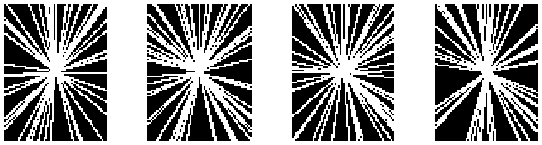
With radially retained sampling, each in our data set consists of all pixels on an Cartesian grid in the Fourier domain that intersect a ray emanating from the origin (each angle corresponds to for a different index ). Figure 1 displays four examples of uniformly random subsets of , sampling the angles of the rays uniformly at random. For radially retained sampling, we refrain from supplementing the subsampled set with any fixed subset; that is, the set is empty. To construct , we generate angles uniformly at random (rounding to the nearest integer), which makes the errors easy to see in the coming figures, yet not too extreme.
With horizontally retained sampling, each in our data set consists of a horizontal line pixels wide on an Cartesian grid in the Fourier domain, with consisting of the integers from to . The subsampled set always includes all horizontal lines ranging from the th lowest frequency to the th lowest frequency (rounding to the nearest integer); that is, the set consists of these low-frequency indices. To construct the remainder of , we generate integers from to uniformly at random (rounding to the nearest integer), which makes the errors easy to see in the coming figures, yet not too extreme. Recall that is a set: each member of occurs only once irrespective of how many times the sampling procedure just described chooses to include the index .
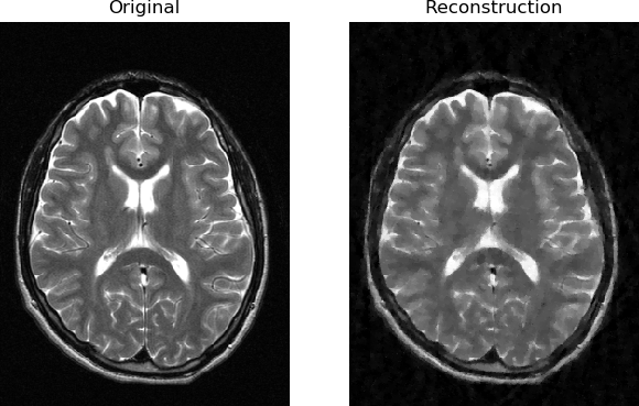
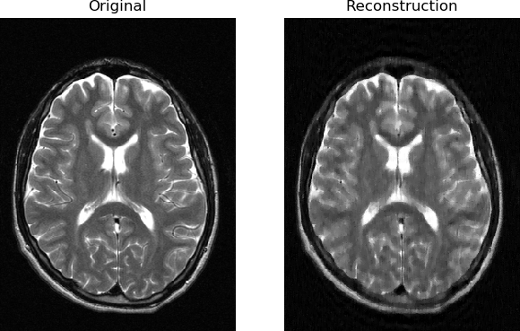
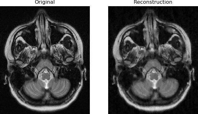
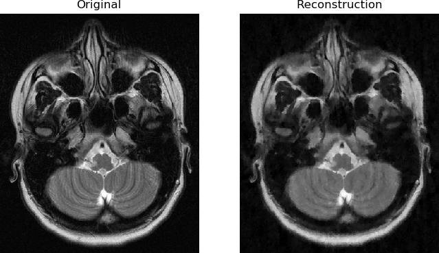
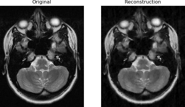
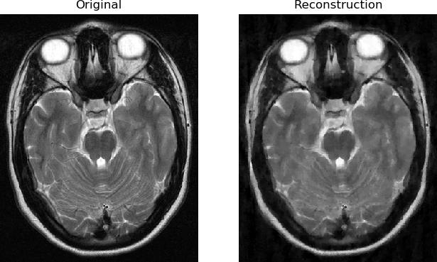
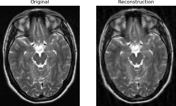
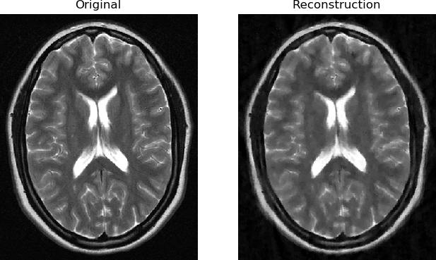
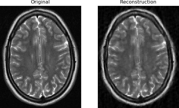
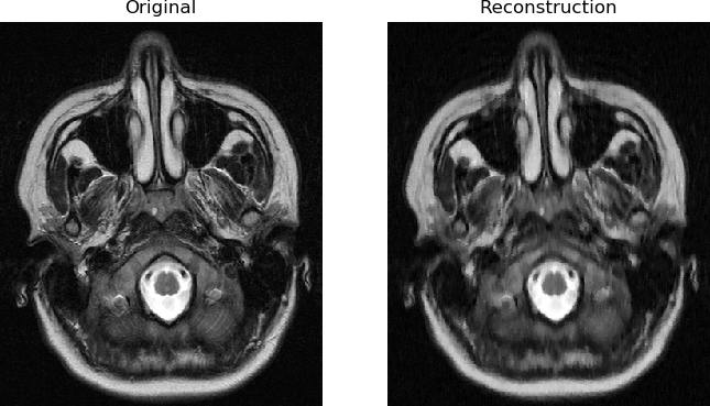
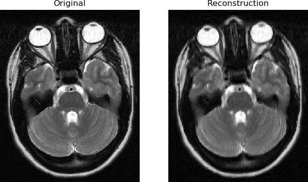
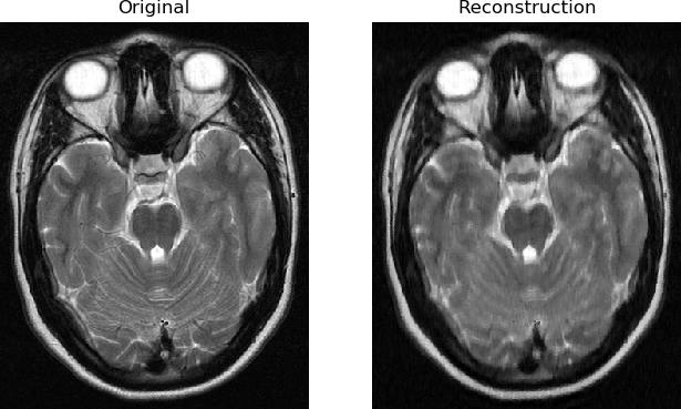
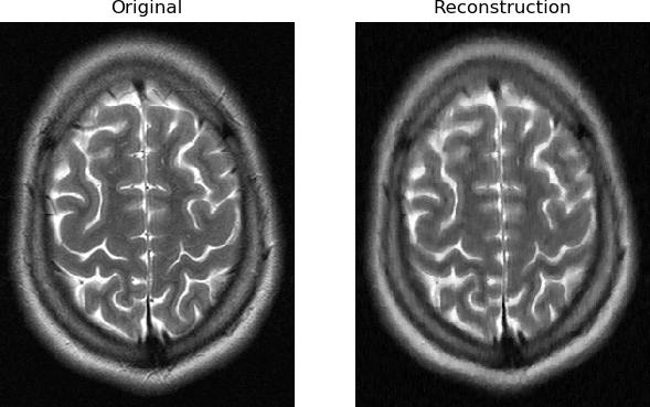
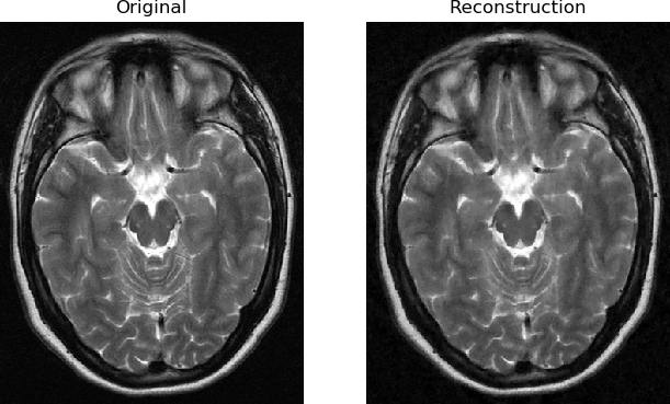
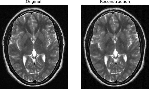
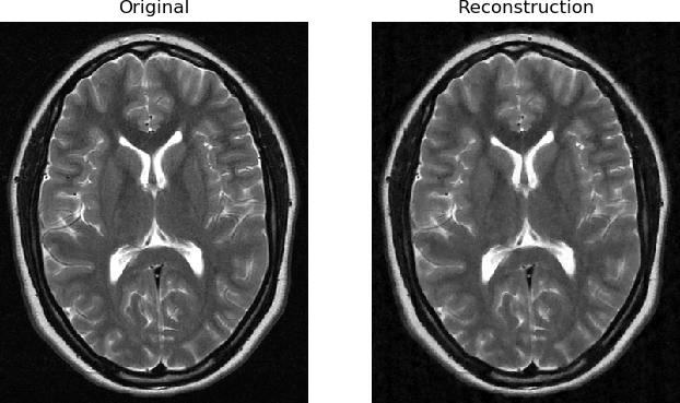
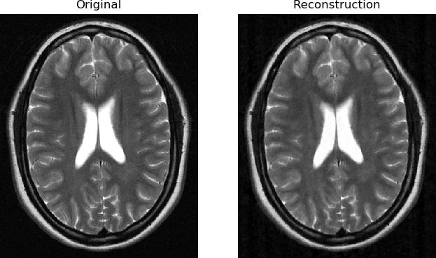
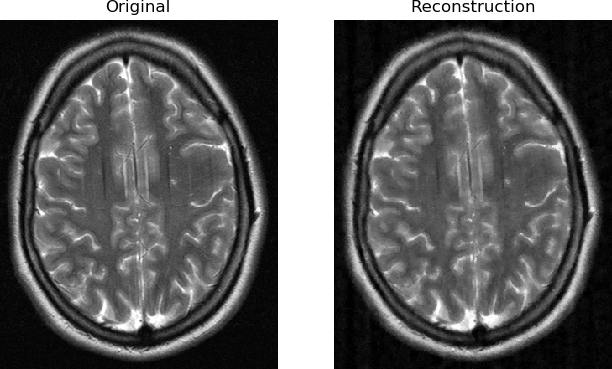
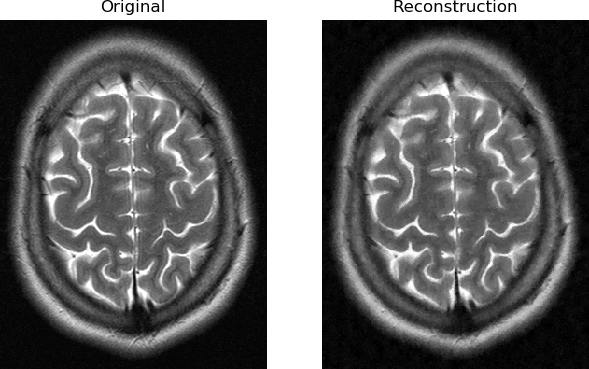
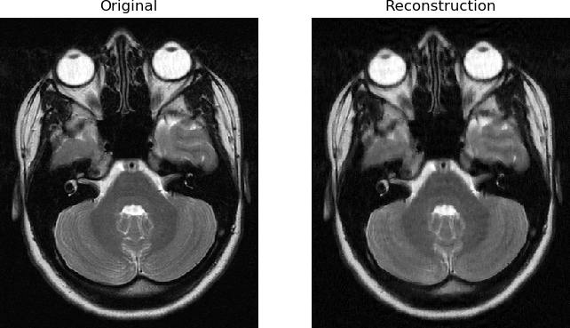
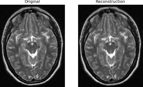
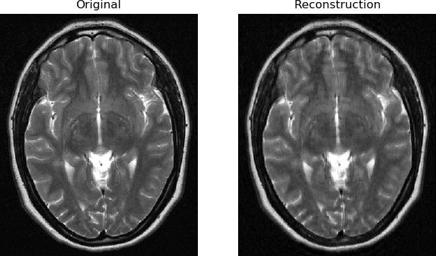
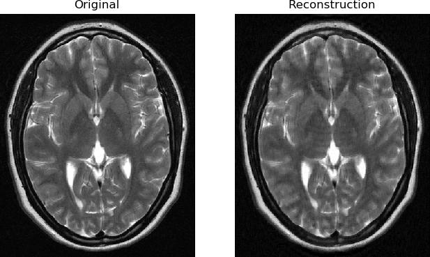
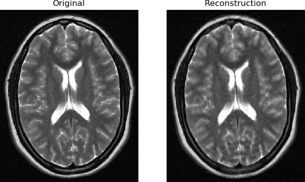
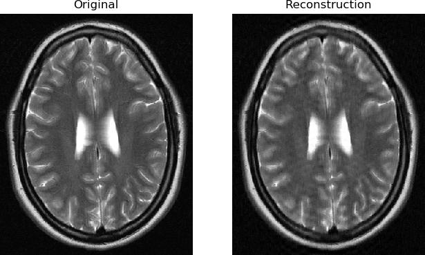
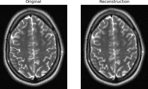
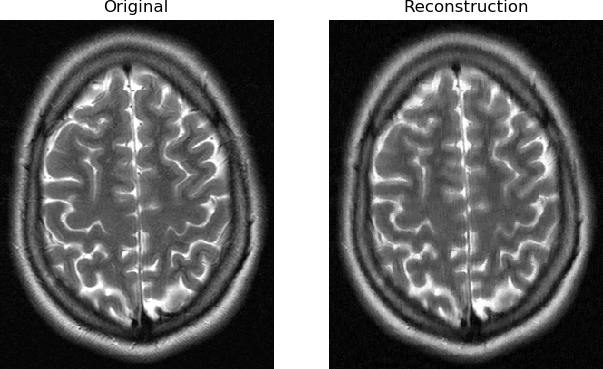
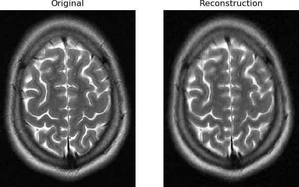
Figures 2 and 3 display results for retaining radial and horizontal lines, respectively, using the same original image. Further examples are available in the appendix. The figures whose captions specify “” use random angles for radially retained sampling and random integers for horizontally retained sampling instead of the random angles and random integers used in all other figures. All figures concern MRI scans of patients’ heads from the data of [3], [4], [5], and [6]. The resolution in pixels of the original image for Figures 2 and 3 is . The resolutions in pixels of the original images for the appendix range from to .
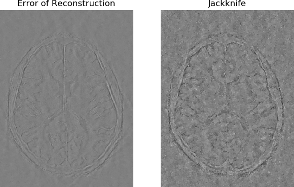
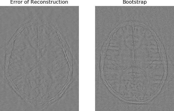
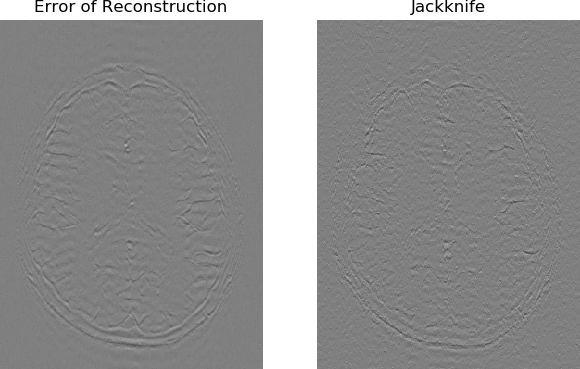
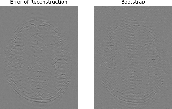
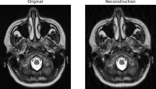
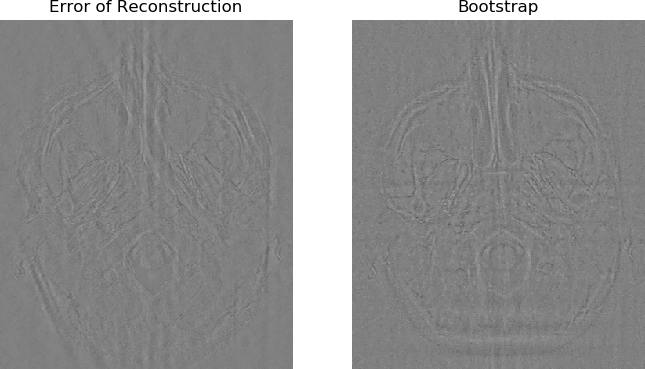
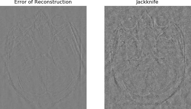
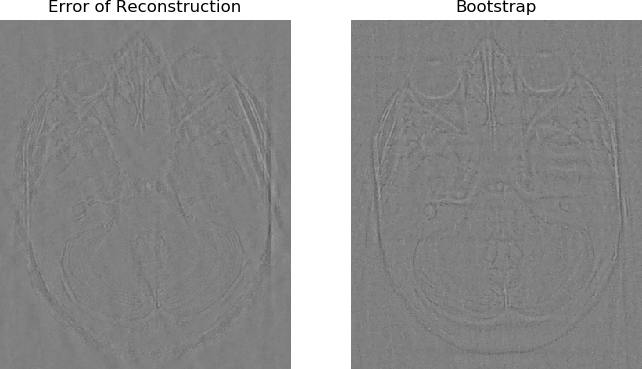
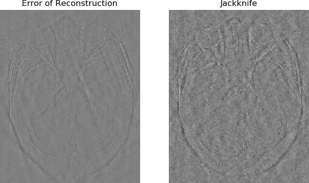
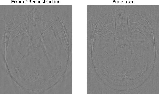
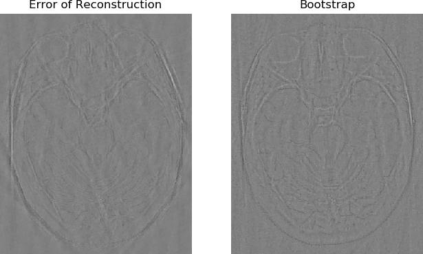
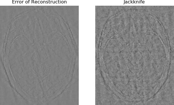
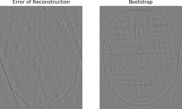
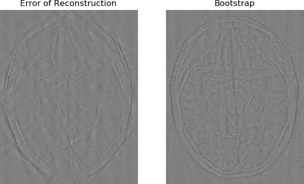
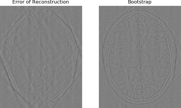
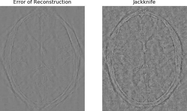
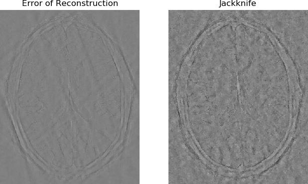
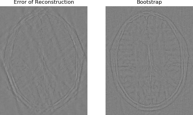
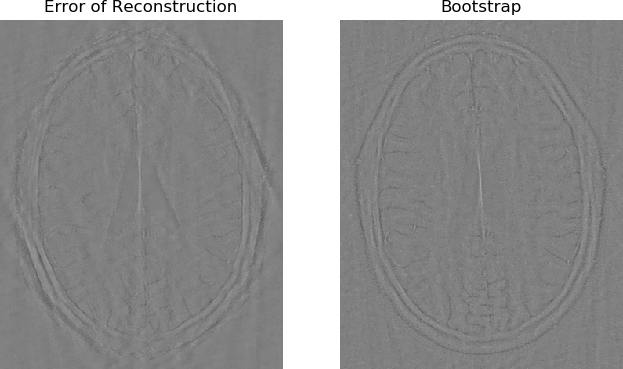
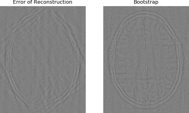
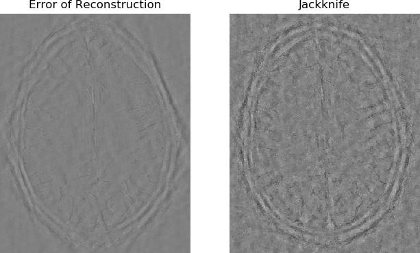
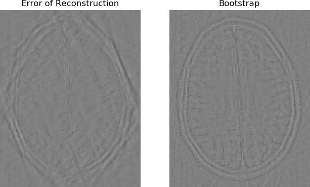
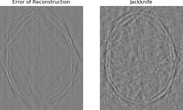
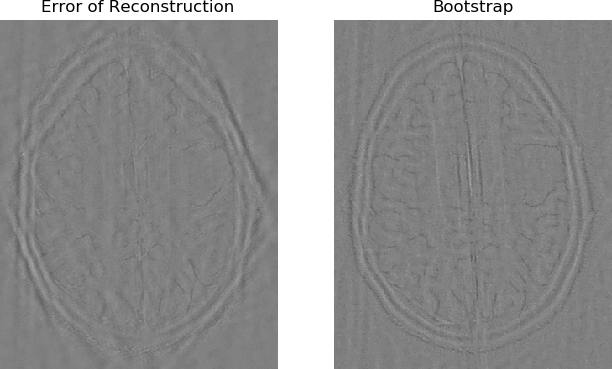
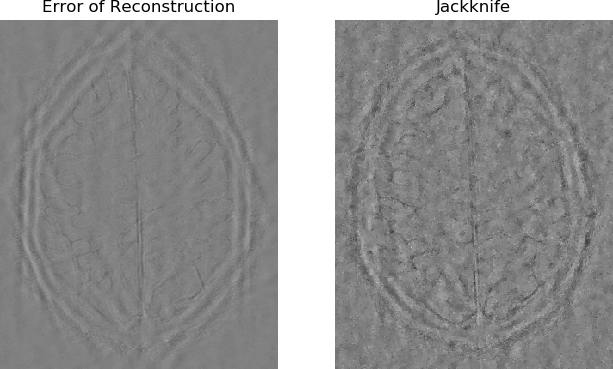
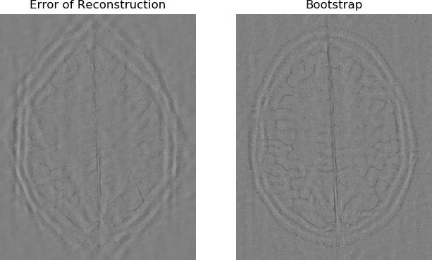
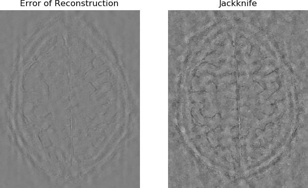
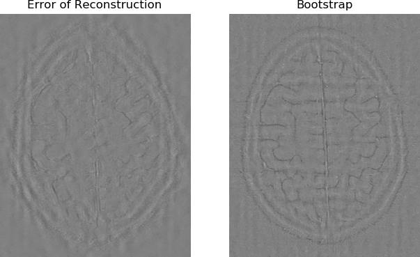
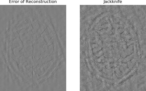
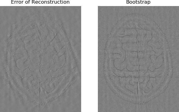
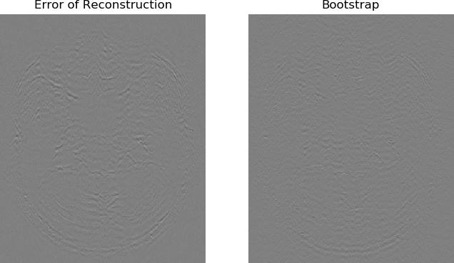
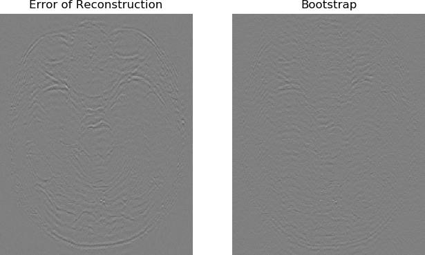
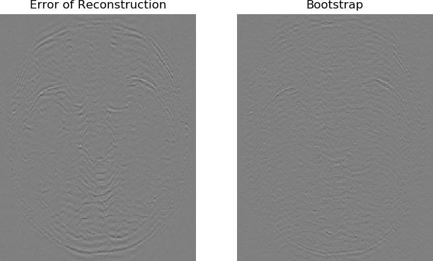
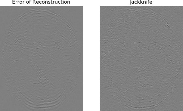
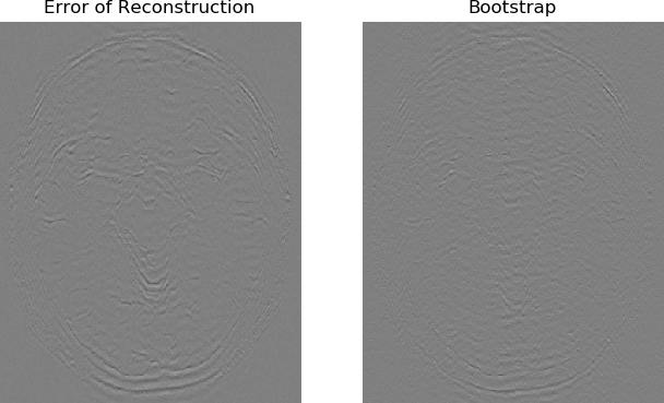
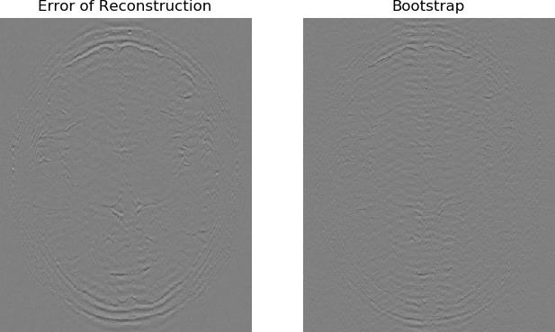
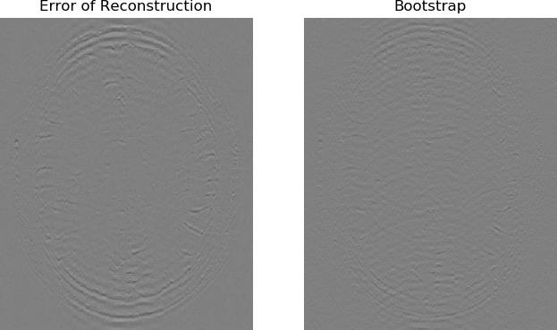
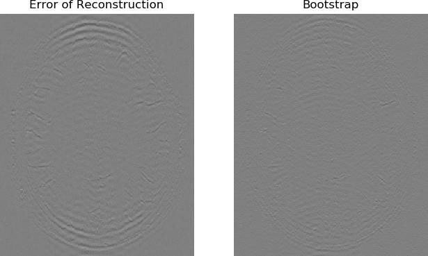
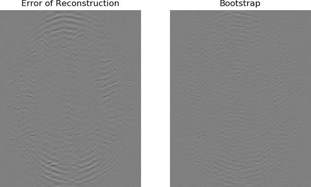
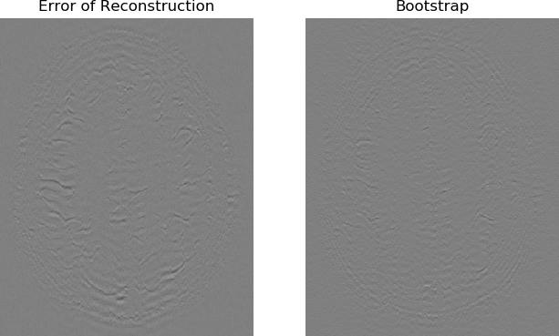
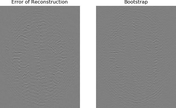
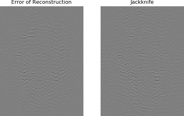
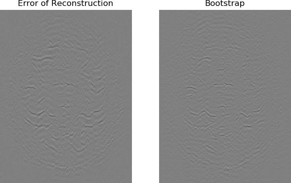
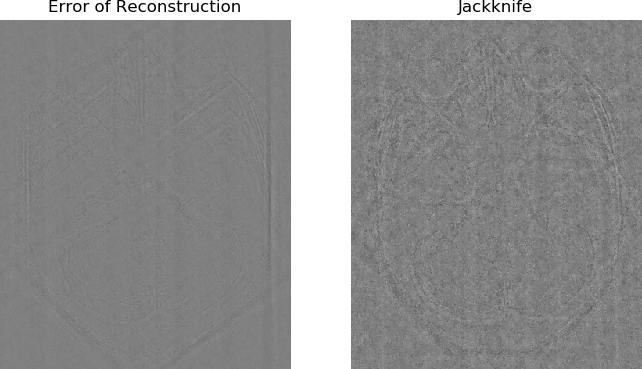
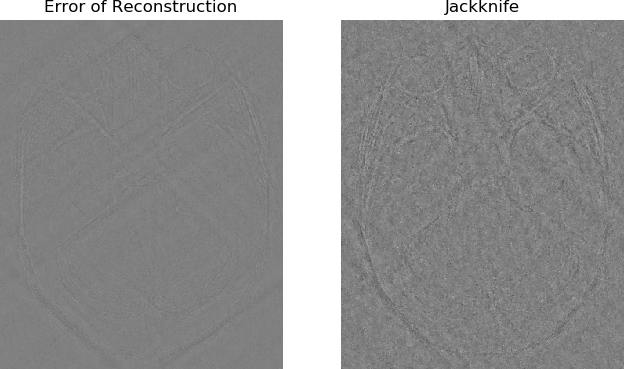
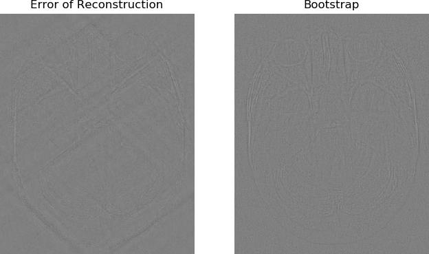
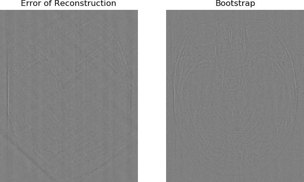
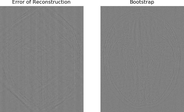
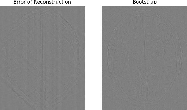
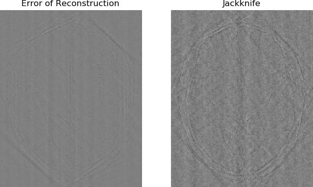
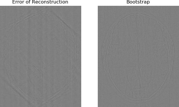
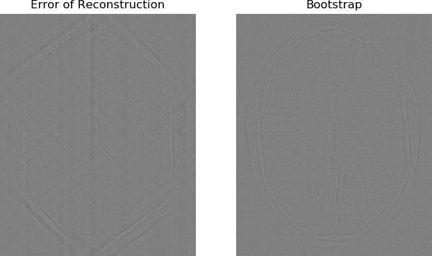
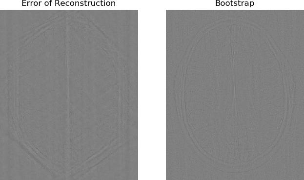
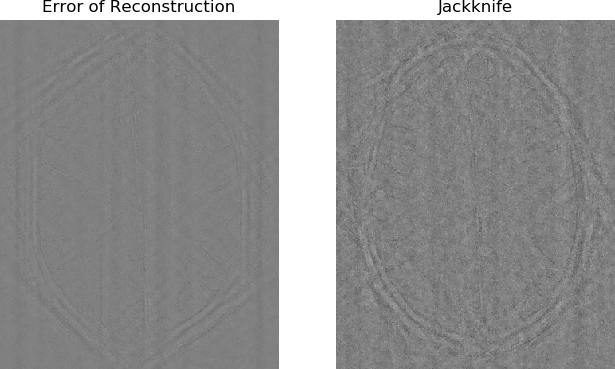
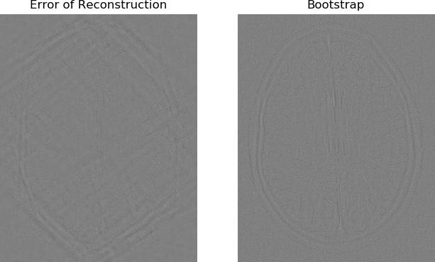
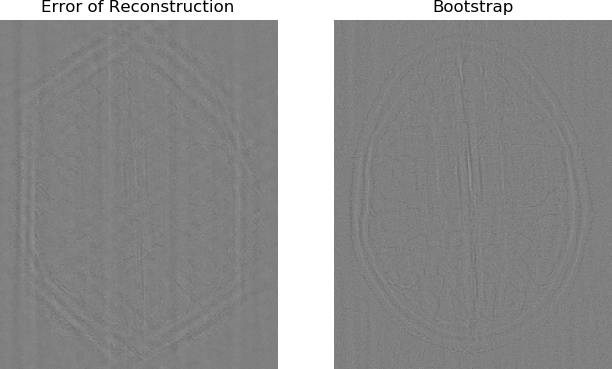
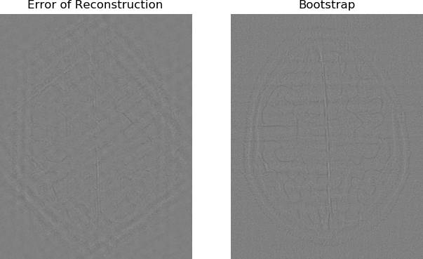
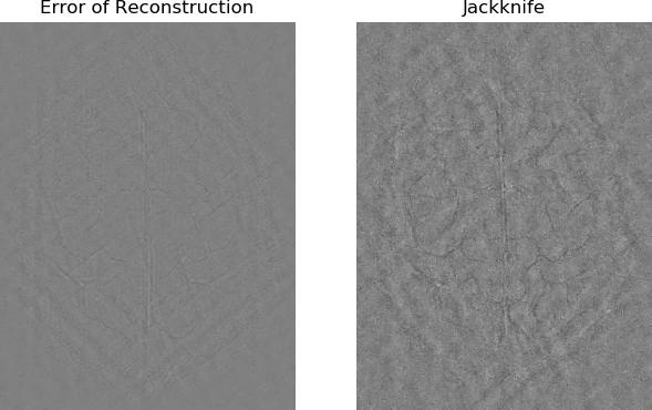
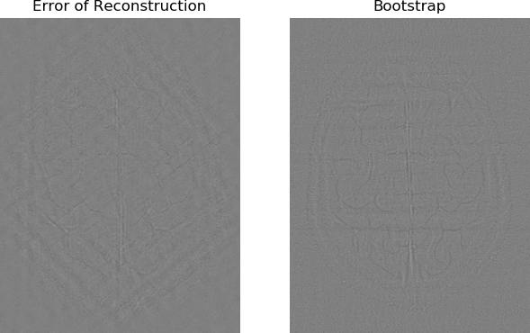
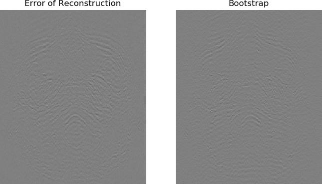
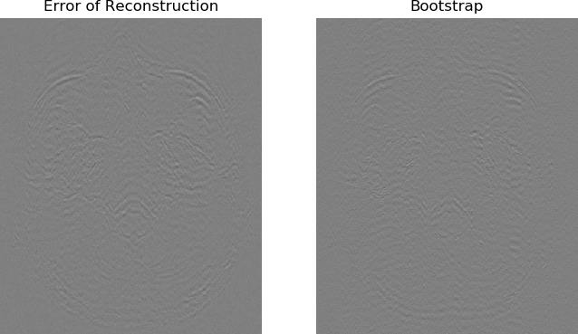
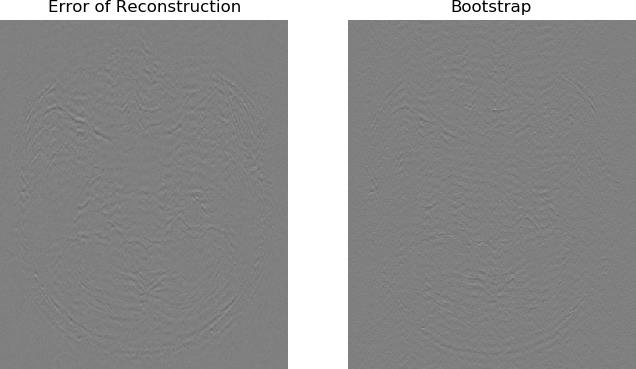
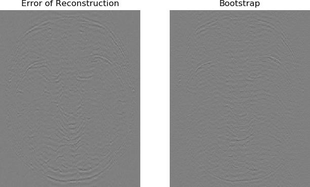
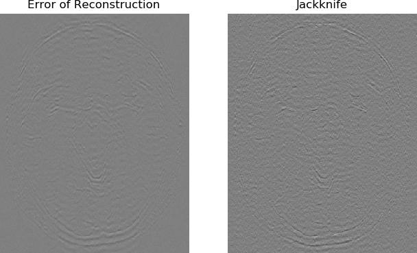
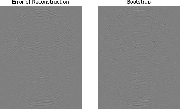
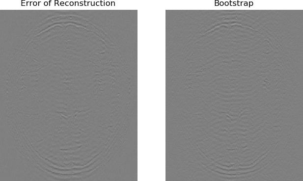
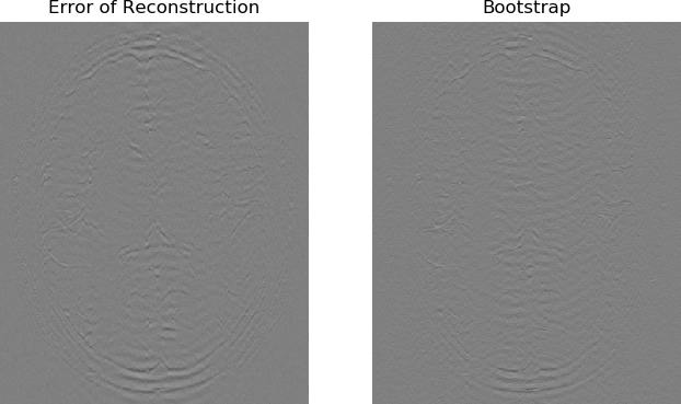
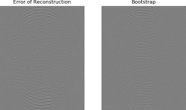
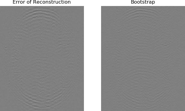
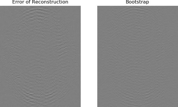
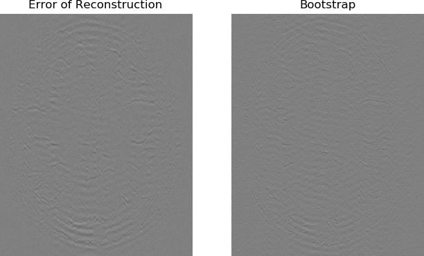
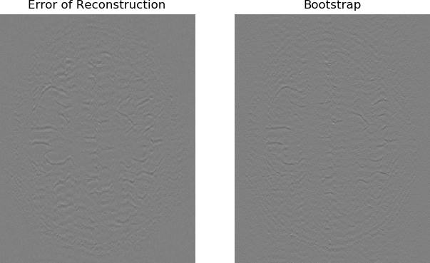
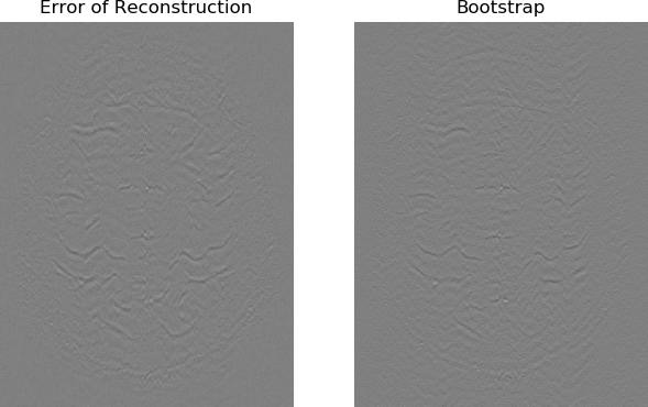
In the figures, “Original” displays the original image, “Reconstruction” displays the reconstruction , “Error of Reconstruction” displays the difference between the original image and the reconstruction, “Jackknife” displays the jackknife from (1), and “Bootstrap” displays the bootstrap from (3). The values of the original pixels are normalized to range from to . In the images “Original” and “Reconstruction,” pure black corresponds to 0 while pure white corresponds to 1. In the images “Error of Reconstruction,” “Jackknife,” and “Bootstrap,” pure white and pure black correspond to the extreme values , whereas 50% gray (halfway to black or to white) corresponds to 0. Thus, in the images displaying errors and potential errors, middling halftone grays correspond to little or no error, while extreme pure white and pure black correspond to more substantial errors.
The jackknife images are generally noisier than the bootstrap images. The bootstrap directly explores parts of the Fourier domain outside the observed measurements, whereas the jackknife is more like a convergence test or a differential approximation to the bootstrap — see, for example, the review of [2]. Both the jackknife and the bootstrap occasionally display artifacts where in fact the reconstruction was accurate. Moreover, they miss some anomalies; if the reconstruction completely washes out a feature of the original image, then neither the jackknife nor the bootstrap can detect the washed-out feature. That said, in most cases they show the actual errors nicely. The estimates bear an uncanny resemblance to the actual errors. Using both the jackknife and the bootstrap may be somewhat conservative, but if the jackknife misses an error, then the bootstrap usually catches it, and vice versa.
Acknowledgements
We would like to thank Florian Knoll, Jerry Ma, Jitendra Malik, Matt Muckley, Mike Rabbat, Dan Sodickson, and Larry Zitnick.
Appendix: Supplementary figures
This appendix supplements the examples of Section 3 with analogous figures for twenty cross-sectional slices through the head of another patient.


References
- [1] R. W. Brown, Y.-C. N. Cheng, E. M. Haacke, M. R. Thompson, and R. Venkatesan, Magnetic Resonance Imaging: Physical Principles and Sequence Design, Wiley-Blackwell, 2nd ed., 2014.
- [2] B. Efron and R. J. Tibshirani, An Introduction to the Bootstrap, CRC Monographs on Statistics & Applied Probability, Chapman & Hall, New York, NY, 1993.
- [3] C. P. Loizou, E. C. Kyriacou, I. Seimenis, M. Pantziaris, S. Petroudi, M. Karaolis, and C. Pattichis, Brain white matter lesion classification in multiple sclerosis subjects for the prognosis of future disability, Intel. Decision Tech. J., 7 (2013), pp. 3–10.
- [4] C. P. Loizou, V. Murray, M. Pattichis, I. Seimenis, M. Pantziaris, and C. Pattichis, Multi-scale amplitude-modulation–frequency-modulation (AM-FM) texture analysis of multiple sclerosis in brain MRI images, IEEE Trans. Inform. Tech. Biomed., 15 (2011), pp. 119–129.
- [5] C. P. Loizou, M. Pantziaris, C. S. Pattichis, and I. Seimenis, Brain MRI image normalization in texture analysis of multiple sclerosis, J. Biomed. Graph. Comput., 3 (2013), pp. 20–34.
- [6] C. P. Loizou, S. Petroudi, I. Seimenis, M. Pantziaris, and C. Pattichis, Quantitative texture analysis of brain white matter lesions derived from T2-weighted MR images in MS patients with clinically isolated syndrome, J. Neuroradiol., 42 (2015), pp. 99–114.
- [7] D. M. Malioutov, S. R. Sanghavi, and A. S. Willsky, Sequential compressed sensing, IEEE J. Select. Topics Signal Proc., 4 (2010), pp. 435–444.
- [8] M. Tao and J. Yang, Alternating direction algorithms for total variation deconvolution in image reconstruction, Tech. Rep. TR0918, Department of Mathematics, Nanjing University, 2009. Available at http://www.optimization-online.org/DB_HTML/2009/11/2463.html.
- [9] J. A. Tropp, Book review: A mathematical introduction to compressive sampling by S. Foucart and H. Rauhut, Bull. Amer. Math. Soc., 54 (2017), pp. 151–165.
- [10] R. Ward, Compressed sensing with cross-validation, IEEE Trans. Inform. Theory, 55 (2009), pp. 5773–5782.
- [11] J. Yang and Y. Zhang, Alternating direction algorithms for -problems in compressive sensing, SIAM J. Sci. Comput., 33 (2011), pp. 250–278.