Testing Selective Influence Directly Using Trackball Movement Tasks

Abstract

Systems factorial technology (SFT; Townsend & Nozawa, 1995) is regarded as a useful tool to diagnose if features (or dimensions) of the investigated stimulus are processed in a parallel or serial fashion. In order to use SFT, one has to assume the speed to process each feature is influenced by that feature only, termed as selective influence (Sternberg, 1969). This assumption is usually untestable as the processing time for a stimulus feature is not observable. Stochastic dominance is traditionally used as an indirect evidence for selective influence (e.g., Townsend & Fifić, 2004). However, one should keep in mind that selective influence may be violated even when stochastic dominance holds. The current study proposes a trackball movement paradigm for a direct test of selective influence. The participants were shown a reference stimulus and a test stimulus simultaneously on a computer screen. They were asked to use the trackball to adjust the test stimulus until it appeared to match the position or shape of the reference stimulus. We recorded the reaction time, the parameters defined the reference stimulus (denoted as $\alpha$ and $\beta$ ), and the parameters defined the test stimulus (denoted as $A$ and $B$). It was expected that the participants implemented the serial AND, parallel AND, or coactive manner to adjust $A$ and $B$, and serial OR and parallel OR strategies were prohibited. We tested selective influence of $\alpha$ and $\beta$ on the amount of time to adjust $A$ and $B$ through testing selective influence of $\alpha$ and $\beta$ on the values of $A$ and $B$ using the linear feasibility test (Dzhafarov & Kujala, 2010). We found that when the test was passed and stochastic dominance held, the inferred architecture was as expected, which was further confirmed by the trajectory of $A$ and $B$ observed in each trial. However, with stochastic dominance only SFT can suggest a prohibited architecture. Our results indicate the proposed method is more reliable for testing selective influence on the processing speed than examining stochastic dominance only.

Keywords: systems factorial technology, selective influence, stochastic dominance

¹ Department of Psychology and Neuroscience, University of Colorado, Boulder, Boulder, CO, USA

² Department of Psychology, National Cheng Kung University, No. 1, University Road, Tainan, Taiwan 701

³ Department of Mathematical Information Technology, University of Jyväskylä, FI-40014 Jyväskylä, Finland

Introduction

A mental architecture is a hypothetical network of mental processes when a cognitive task is being performed by a subject. Considering a stimulus having only two features $\alpha$ and $\beta$. Let us assume there is a channel to process the information of $\alpha$ and another channel to process the information of $\beta$. There are numerous ways to arrange the two channels. One can inspect three fundamental characteristics of the arrangements, that are architecture (serial vs. parallel), stopping rule (OR vs. AND), and capacity (limited, unlimited vs. super). A serial architecture processes one channel after the preceding channel is completely executed. A parallel architecture starts to process all the channels simultaneously but can terminate them at different times. The OR rule means that the entire processing can be completed as soon as any one of the channels is complete. If all processes must be completely executed to ensure a response, then it is the AND rule. Capacity measures the efficiency of information processing as the workload, i.e., number of channels varies. When executing a given channel is not affected by adding an additional channel, the capacity is unlimited. Super capacity indicates that processing efficiency of individual channels actually increases as the workload is increased. Limited capacity indicates that the processing efficiency decreases with the increased workload. Those properties can be understood by inspecting the distributional behavior of response/reaction time (RT) in a double-factorial paradigm (DFP) in the framework of systems factorial technology (SFT; Townsend & Nozawa, 1995; for further development, see Schweickert, Giorgini, & Dzhafarov, 2000; Dzhafarov, Schweickert, & Sung, 2004; Yang, Fifić, & Townsend, 2013; Zhang & Dzhafarov, 2015; Little, Altieri, Fifić, & Yang, 2017). There are two critical types of manipulation that comprise the DFP: manipulation of workload and manipulation of stimulus salience. This paradigm includes a full factorial combination of the two types of manipulation, each incorporating two levels for each stimulus feature. For instance, in a visual detection task two dots (denoted as $\alpha$ and $\beta$) are presented to the subjects, one on the left and the other on the right. The researcher manipulates the stimulus salience by choosing two different levels of brightness for each dot, level one for less bright and level two for bright. So there are four stimuli for this type of manipulation: $\alpha_{1}\beta_{1}$, $\alpha_{1}\beta_{2}$, $\alpha_{2}\beta_{1}$, and $\alpha_{2}\beta_{2}$. The manipulation of workload can be realized by tuning each dot on and off. So in some trials only the left dot or the right dot is shown. This type of manipulation introduces four additional stimuli to the experiment: $\alpha_{0}\beta_{1}$, $\alpha_{0}\beta_{2}$, $\alpha_{1}\beta_{0}$, and $\alpha_{2}\beta_{0}$, where the subscript 0 indicates the corresponding dot is off. The trials with only one dot displays are named single-channel trials. The trials with two dots display are named double-channel trials. So far SFT has been widely used to investigate mental architectures implemented in various cognitive tasks with short RT, such as the simple detection task (Townsend & Nozawa, 1995), Stroop task (Eidels, Townsend, & Algom, 2010), Gestalt principles (Eidels, Townsend, & Pomerantz, 2008), visual search (Fifić, Townsend, & Eidels, 2008), short-term memory search (Townsend & Fifić, 2004), face perception (Fifić & Townsend, 2010; Wenger & Townsend, 2001; Yang, Fifić, Chang, & Little, 2018), attention (Yang, 2017), change detection (Yang, 2011), audiovisual detection (Yang, Altieri, & Little, 2018), categorization (Fifić, Little, & Nosofsky, 2010), and even in the clinical domain (Johnson, Blaha, Houpt, & Townsend, 2010; Altieri & Yang, 2016).

In order to implement SFT, one has to impose three assumptions on the investigated system: ordering of the RT distributions (Townsend & Schweickert, 1989), selective influence (Sternberg, 1969), and subject’s adherence to a single type of mental architecture. Ordering of the RT distributions is expressed as the ordering of survival functions:

$$S_{\alpha_{1}}(t) \geq S_{\alpha_{2}}(t),$$

$$S_{\beta_{1}}(t) \geq S_{\beta_{2}}(t).$$ (1)

$S_{\alpha_{i}}(t)$ is the survival function for $T_{\alpha_{i}},i\in\left\{1,2\right\}$, which is the duration for channel $\alpha$ at level $i$, and $S_{\beta_{j}}(t)$ is the survival function for $T_{\beta_{j}},j\in\left\{1,2\right\}$, which is the duration for channel $\beta$ at level $j$. The ordering assumption can be easily satisfied empirically as one can for instance manipulate the brightness of a stimulus that the less bright stimulus is processed slower than the bright one.

SFT requires selective influence which can be understood as the duration for channel $\alpha$ is affected by the changing of $\alpha$ but not the changing of $\beta$, and the duration for channel $\beta$ is affected by the changing of $\beta$ but not the changing of $\alpha$. It is written as

$$(T_{\alpha},T_{\beta})\looparrowleft(\alpha,\beta).$$ (2)

Dzhafarov and Kujala (2010) proposed a rigorous definition for it: Random variables $T_{\alpha}$ and $T_{\beta}$ are selectively influenced by $\alpha$ and $\beta$, if and only if there are measurable functions $g_{\alpha}$ and $g_{\beta}$ and a random entity $C$ whose distribution is independent of $\alpha$ and $\beta$, such that $(T_{\alpha},T_{\beta})\sim(g_{\alpha}(\alpha,C),g_{\beta}(\beta,C))$, where $\sim$ stands for "is distributed as". The random entity $C$, in psychology, can be resolution of the monitor, which is apparently independent of stimulus features $\alpha$ and $\beta$, but influences $T_{\alpha}$ and $T_{\beta}$ simultaneously. Please note Dzhafarov and Kujala’s definition of selective influence is not limited in the field of psychology: $\alpha$ and $\beta$ can be two external factors in any system and $T_{\alpha}$ and $T_{\beta}$ are the random variables in response to the external factors. The readers should keep in mind in the framework of SFT the notion of selective influence is confined on the relation between stimulus features and the durations to process those features.

Dzhafarov and Kujala (2010) also proposed an equivalent definition: Selective influence (2) holds if and only if there exists a jointly distributed quadruple $(H_{\alpha_{1}},H_{\alpha_{2}},H_{\beta_{1}},H_{\beta_{2}})$, such that

$$(H_{\alpha_{i}},H_{\beta_{j}})\sim(T_{\alpha_{i}},T_{\beta_{j}})\mid_{\alpha_{i}\beta_{j}},$$

where $(T_{\alpha_{i}},T_{\beta_{j}})\mid_{\alpha_{i}\beta_{j}}$ represents the jointly distributed $T_{\alpha_{i}}$ and $T_{\beta_{j}}$ conditioned on the stimulus $\alpha_{i}\beta_{j}$. Dzhafarov and Kujala (2010) developed the linear feasibility test (LFT) to establish or falsify selective influence. Let us assume that $T_{\alpha}$ has $m$ possible values: $\left\{a_{1},a_{2},...,a_{m}\right\}$ and $T_{\beta}$ has $n$ possible values: $\left\{b_{1},b_{2},...,b_{n}\right\}$. Let us write the joint probability for the vector $(H_{\alpha_{1}},H_{\alpha_{2}},H_{\beta_{1}},H_{\beta_{2}})$ as

$$\Pr\left(H_{\alpha_{1}}=a_{\alpha_{1}},H_{\alpha_{2}}=a_{\alpha_{2}},H_{\beta_{1}}=b_{\beta_{1}},H_{\beta_{2}}=b_{\beta_{2}}\right)=Q_{a_{\alpha_{1}}a_{\alpha_{2}}b_{\beta_{1}}b_{\beta_{2}}},$$

where $a_{\alpha_{1}},a_{\alpha_{2}}\in\left\{a_{1},a_{2},...,a_{m}\right\}$ and $b_{\beta_{1}},b_{\beta_{2}}\in\left\{b_{1},b_{2},...,b_{n}\right\}$ with constraints

$$Q_{a_{\alpha_{1}}a_{\alpha_{2}}b_{\beta_{1}}b_{\beta_{2}}}\geq 0,$$

such that

$$\Pr\left(H_{\alpha_{1}}=a_{\alpha_{1}},H_{\beta_{1}}=b_{\beta_{1}}\right) =\sum_{a_{\alpha_{2}}b_{\beta_{2}}}Q_{a_{\alpha_{1}}a_{\alpha_{2}}b_{\beta_{1}}b_{\beta_{2}}}=\Pr\left(T_{\alpha_{1}}=a_{\alpha_{1}},T_{\beta_{1}}=b_{\beta_{1}}\right)\mid_{\alpha_{1}\beta_{1}},$$

$$\Pr\left(H_{\alpha_{1}}=a_{\alpha_{1}},H_{\beta_{2}}=b_{\beta_{2}}\right) =\sum_{a_{\alpha_{2}}b_{\beta_{1}}}Q_{a_{\alpha_{1}}a_{\alpha_{2}}b_{\beta_{1}}b_{\beta_{2}}}=\Pr\left(T_{\alpha_{1}}=a_{\alpha_{1}},T_{\beta_{2}}=b_{\beta_{2}}\right)\mid_{\alpha_{1}\beta_{2}},$$

$$\Pr\left(H_{\alpha_{2}}=a_{\alpha_{2}},H_{\beta_{1}}=b_{\beta_{1}}\right) =\sum_{a_{\alpha_{1}}b_{\beta_{2}}}Q_{a_{\alpha_{1}}a_{\alpha_{2}}b_{\beta_{1}}b_{\beta_{2}}}=\Pr\left(T_{\alpha_{2}}=a_{\alpha_{2}},T_{\beta_{1}}=b_{\beta_{1}}\right)\mid_{\alpha_{2}\beta_{1}},$$

$$\Pr\left(H_{\alpha_{2}}=a_{\alpha_{2}},H_{\beta_{2}}=b_{\beta_{2}}\right) =\sum_{a_{\alpha_{1}}b_{\beta_{1}}}Q_{a_{\alpha_{1}}a_{\alpha_{2}}b_{\beta_{1}}b_{\beta_{2}}}=\Pr\left(T_{\alpha_{2}}=a_{\alpha_{2}},T_{\beta_{2}}=b_{\beta_{2}}\right)\mid_{\alpha_{2}\beta_{2}}.$$ (3)

If the nonnegative solution for the $Q$ variables that satisfies (3) exists, we say LFT is passed and selective influence (2) is established, otherwise selective influence is falsified.

Marginal selectivity is a necessary condition for selective influence. It states that the marginal distribution of $T_{\alpha}$ does not depend on $\beta$ and the marginal distribution of $T_{\beta}$ does not depend on $\alpha$. It can be mathematically written as

$$\sum_{b_{\beta_{1}}}\Pr\left(T_{\alpha_{1}}=a_{\alpha_{1}},T_{\beta_{1}}=b_{\beta_{1}}\right)\mid_{\alpha_{1}\beta_{1}} =\sum_{b_{\beta_{2}}}\Pr\left(T_{\alpha_{1}}=a_{\alpha_{1}},T_{\beta_{2}}=b_{\beta_{2}}\right)\mid_{\alpha_{1}\beta_{2}},$$

$$\sum_{b_{\beta_{1}}}\Pr\left(T_{\alpha_{2}}=a_{\alpha_{2}},T_{\beta_{1}}=b_{\beta_{1}}\right)\mid_{\alpha_{2}\beta_{1}} =\sum_{b_{\beta_{2}}}\Pr\left(T_{\alpha_{2}}=a_{\alpha_{2}},T_{\beta_{2}}=b_{\beta_{2}}\right)\mid_{\alpha_{2}\beta_{2}},$$

$$\sum_{a_{\alpha_{1}}}\Pr\left(T_{\alpha_{1}}=a_{\alpha_{1}},T_{\beta_{1}}=b_{\beta_{1}}\right)\mid_{\alpha_{1}\beta_{1}} =\sum_{a_{\alpha_{2}}}\Pr\left(T_{\alpha_{2}}=a_{\alpha_{2}},T_{\beta_{1}}=b_{\beta_{1}}\right)\mid_{\alpha_{2}\beta_{1}},$$

$$\sum_{a_{\alpha_{1}}}\Pr\left(T_{\alpha_{1}}=a_{\alpha_{1}},T_{\beta_{1}}=b_{\beta_{2}}\right)\mid_{\alpha_{1}\beta_{2}} =\sum_{a_{\alpha_{2}}}\Pr\left(T_{\alpha_{2}}=a_{\alpha_{2}},T_{\beta_{1}}=b_{\beta_{2}}\right)\mid_{\alpha_{2}\beta_{2}}.$$ (4)

(3) implies marginal selectivity (4). If marginal selectivity is violated, the nonnegative solution for (3) does not exist.

Table 1 gives an example of joint probabilities $\Pr\left(T_{\alpha_{i}}=a_{\alpha_{i}},T_{\beta_{j}}=b_{\beta_{j}}\right)\mid_{\alpha_{i}\beta_{j}}$, where $i,j\in\left\{1,2\right\}$ and $m=n=2$. The numbers outside the grids are marginal probabilities.

Table 1: An example of joint probabilities of $(T_{\alpha_{i}},T_{\beta_{j}})$ given stimulus $\alpha_{i}\beta_{j}$, $i,j\in\left\{1,2\right\}$.

$\alpha_{1}\beta_{1}$	$T_{\beta_{1}}=b_{1}$	$T_{\beta_{1}}=b_{2}$
$T_{\alpha_{1}}=a_{1}$	.2	.2	.4
$T_{\alpha_{1}}=a_{2}$	.1	.5	.6
	.3	.7

$\alpha_{1}\beta_{2}$	$T_{\beta_{2}}=b_{1}$	$T_{\beta_{2}}=b_{2}$
$T_{\alpha_{1}}=a_{1}$	.3	.1	.4
$T_{\alpha_{1}}=a_{2}$	.4	.2	.6
	.7	.3

$\alpha_{2}\beta_{1}$	$T_{\beta_{1}}=b_{1}$	$T_{\beta_{1}}=b_{2}$
$T_{\alpha_{2}}=a_{1}$	.1	.5	.6
$T_{\alpha_{2}}=a_{2}$	.2	.2	.4
	.3	.7

$\alpha_{2}\beta_{2}$	$T_{\beta_{2}}=b_{1}$	$T_{\beta_{2}}=b_{2}$
$T_{\alpha_{2}}=a_{1}$	.4	.2	.6
$T_{\alpha_{2}}=a_{2}$	.3	.1	.4
	.7	.3

This example satisfies marginal selectivity since the conditions in (4) are met. Substituting the joint probabilities in Table 1 into (3),

$$\left(\begin{array}[]{cccccccccccccccc}1&1&0&0&1&1&0&0&0&0&0&0&0&0&0&0\\ 0&0&1&1&0&0&1&1&0&0&0&0&0&0&0&0\\ 0&0&0&0&0&0&0&0&1&1&0&0&1&1&0&0\\ 0&0&0&0&0&0&0&0&0&0&1&1&0&0&1&1\\ 1&0&1&0&1&0&1&0&0&0&0&0&0&0&0&0\\ 0&1&0&1&0&1&0&1&0&0&0&0&0&0&0&0\\ 0&0&0&0&0&0&0&0&1&0&1&0&1&0&1&0\\ 0&0&0&0&0&0&0&0&0&1&0&1&0&1&0&1\\ 1&1&0&0&0&0&0&0&1&1&0&0&0&0&0&0\\ 0&0&1&1&0&0&0&0&0&0&1&1&0&0&0&0\\ 0&0&0&0&1&1&0&0&0&0&0&0&1&1&0&0\\ 0&0&0&0&0&0&1&1&0&0&0&0&0&0&1&1\\ 1&0&1&0&0&0&0&0&1&0&1&0&0&0&0&0\\ 0&1&0&1&0&\text{0}&0&0&0&1&0&1&0&0&0&0\\ 0&0&0&0&1&0&1&0&0&0&0&0&1&0&1&0\\ 0&0&0&0&0&1&0&1&0&0&0&0&0&1&0&1\end{array}\right)\left(\begin{array}[]{c}Q_{a_{1}a_{1}b_{1}b_{1}}\\ Q_{a_{1}a_{1}b_{1}b_{2}}\\ Q_{a_{1}a_{1}b_{2}b_{1}}\\ Q_{a_{1}a_{1}b_{2}b_{2}}\\ Q_{a_{1}a_{2}b_{1}b_{1}}\\ Q_{a_{1}a_{2}b_{1}b_{2}}\\ Q_{a_{1}a_{2}b_{2}b_{1}}\\ Q_{a_{1}a_{2}b_{2}b_{2}}\\ Q_{a_{2}a_{1}b_{1}b_{1}}\\ Q_{a_{2}a_{1}b_{1}b_{2}}\\ Q_{a_{2}a_{1}b_{2}b_{1}}\\ Q_{a_{2}a_{1}b_{2}b_{2}}\\ Q_{a_{2}a_{2}b_{1}b_{1}}\\ Q_{a_{2}a_{2}b_{1}b_{2}}\\ Q_{a_{2}a_{2}b_{2}b_{1}}\\ Q_{a_{2}a_{2}b_{2}b_{2}}\end{array}\right)=\left(\begin{array}[]{c}.2\\ .2\\ .1\\ .5\\ .3\\ .1\\ .4\\ .2\\ .1\\ .5\\ .2\\ .2\\ .4\\ .2\\ .3\\ .1\end{array}\right),$$

the nonnegative solution

$$(Q_{a_{1}a_{1}b_{1}b_{1}},\,Q_{a_{1}a_{1}b_{1}b_{2}},\,\ldots,\,Q_{a_{2}a_{2}b_{2}b_{2}})^{T}$$

$$=(0,0,0,0,.1,.1,.2,0,0,.1,.4,.1,0,0,0,0)^{T}$$

establishes selective influence in this example.

With the assumption of selective influence, as one manipulates the features of the interested stimulus, the durations influenced by these features vary and consequently the overall duration is changed as well. With these factorial manipulations, each mental architecture has a distributional pattern of RT that is different from other architectures. $T_{\alpha}$ and $T_{\beta}$ are usually unobservable in empirical studies, so selective influence of $\alpha$ and $\beta$ on $T_{\alpha}$ and $T_{\beta}$ cannot be tested directly. By imposing the assumption of selective influence, ordering of the RT distributions is equivalent to the four inequalities termed as stochastic dominance:

$$S_{\alpha_{1}\beta_{1}}(t) \geq S_{\alpha_{2}\beta_{1}}(t),$$

$$S_{\alpha_{1}\beta_{2}}(t) \geq S_{\alpha_{2}\beta_{2}}(t),$$

$$S_{\alpha_{1}\beta_{1}}(t) \geq S_{\alpha_{1}\beta_{2}}(t),$$

$$S_{\alpha_{2}\beta_{1}}(t) \geq S_{\alpha_{2}\beta_{2}}(t).$$ (5)

$S_{\alpha_{i}\beta_{j}}(t)$ is the survival function for $T_{\alpha_{i}\beta_{j}}$, which is the overall duration to process the stimulus $\alpha_{i}\beta_{j}$. $T_{\alpha_{i}\beta_{j}}$ is usually observable, therefore stochastic dominance is traditionally used to test selective influence (Townsend & Nozawa, 1995; Eidels, Townsend, & Algom, 2010; Eidels, Townsend, & Pomerantz, 2008; Fifić, Townsend, & Eidels, 2008; Townsend & Fifić, 2004; Fifić & Townsend, 2010; Wenger & Townsend, 2001; Johnson, Blaha, Houpt, & Townsend, 2010). However, one should keep in mind that selective influence may be violated even when stochastic dominance holds. Strictly speaking, stochastic dominance is only a necessary condition for selective influence combined with ordering of RT distributions.

The third assumption states the subject maintains a single type of mental architecture from trial to trial. This assumption could be invalid as one may implement parallel AND for one trial and switch to serial AND in another trial. In psychological research, it is usually impossible to track the mental architecture in each trial.

Three important properties were constructed in the framework of SFT:

• Mean Interaction Contrast (MIC)

$$\mathrm{MIC}(t)=\overline{T}_{\alpha_{1}\beta_{1}}-\overline{T}_{\alpha_{1}\beta_{2}}-\overline{T}_{\alpha_{2}\beta_{1}}+\overline{T}_{\alpha_{2}\beta_{2}},$$

where $\overline{T}_{\alpha_{i}\beta_{j}}$ stands for the mean of $T_{\alpha_{i}\beta_{j}}$.

• Survivor Interaction Contrast (SIC)

$$\mathrm{SIC}(t)=S_{\alpha_{1}\beta_{1}}(t)-S_{\alpha_{1}\beta_{2}}(t)-S_{\alpha_{2}\beta_{1}}(t)+S_{\alpha_{2}\beta_{2}}(t).$$

Four different combinations of architecture and stopping rule are of the greatest traditional interest. They are serial OR, serial AND, parallel OR, and parallel AND (Figure 1(a)). The overall duration for each model is a function of $T_{\alpha}$ and $T_{\beta}$. They are $T_{\alpha\beta}=T_{\alpha}$ or $T_{\beta}$, $T_{\alpha\beta}=T_{\alpha}+T_{\beta}$, $T_{\alpha\beta}=\mathrm{min}(T_{\alpha},T_{\beta})$, and $T_{\alpha\beta}=\mathrm{max}(T_{\alpha},T_{\beta})$, respectively. In addition to the four models, the model with the information from each parallel channel pooled toward a single decision is coactive. Coactive processing is a special case of parallel models. It was previously proved that for a serial OR model, both MIC = 0 and SIC = 0 across time. For a serial AND model, MIC is zero and SIC fluctuates from negative to positive and the sum of areas of its negative part and positive part is zero. For a parallel OR model, both MIC and SIC are positive. For a parallel AND model, both MIC and SIC are negative. For a coactive model, MIC is positive and SIC fluctuates from negative to positive and the area of the negative part is smaller than that of the positive part. Having different characteristic patterns of MIC and SIC, one can diagnose the mental architecture out of the five candidate models (Figure 1(b)).

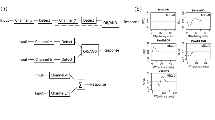
Figure 1: (a) Several classical mental architectures. (b) Characteristic behavior of SIC and MIC for those architectures conditional on the three assumptions (Yang, Fifić, & Townsend, 2013).

• Capacity (C)

In Townsend and Wenger (2004)’s paper, the capacity coefficients were developed using temporal variables. For the AND stopping rule,

• $$\mathrm{C}_{\mathrm{AND}}(t)=\frac{K_{\alpha}(t)+K_{\beta}(t)}{K_{\alpha\beta}(t)},$$ (6)

where $K(t)=\mathrm{ln}(F(t))=\mathrm{ln}(1-S(t))$. For the OR stopping rule,

• $$\mathrm{C}_{\mathrm{OR}}(t)=\frac{H_{\alpha\beta}(t)}{H_{\alpha}(t)+H_{\beta}(t)},$$ (7)

where $H(t)=\int_{0}^{t}h(t)dt=\int_{0}^{t}\frac{f(t)}{S(t)}dt$, where $f(t)$ is the density function. If $\mathrm{C_{AND/OR}}(t)>1$, the capacity is super; if $\mathrm{C_{AND/OR}}(t)=1$, the capacity is unlimited; if $\mathrm{C_{AND/OR}}(t)<1$, the capacity is limited.

In this article we propose a trackball movement paradigm that can test the assumptions that are usually untestable in other paradigms. It includes two tasks: the dot position reproduction task (Experiments 1(a), 1(b), and 1(c)) and the floral shape reproduction task (Experiments 2(a), 2(b), and 2(c)). The participants were shown a reference stimulus and a test stimulus simultaneously on a computer screen. They were asked to use the trackball to adjust the test stimulus until it appeared to match the position or shape of the reference stimulus. There were two parameters defined the reference stimulus (denoted as $\alpha$ and $\beta$ ) and two parameters defined the test stimulus (denoted as $A$ and $B$). So essentially the task goal was to match $\alpha$ and $\beta$ by adjusting $A$ and $B$. We tested selective influence of $\alpha$ and $\beta$ on the amount of time to adjust $A$ and $B$ through testing selective influence of $\alpha$ and $\beta$ on the values of $A$ and $B$ using LFT. We found that when the test was passed and stochastic dominance held, the inferred architecture about the adjustment of $A$ and $B$ was as expected (either parallel AND or coactive), which was further confirmed by the trajectory of $A$ and $B$ observed in each trial. The trajectory also confirmed the assumption that the subjects maintained a stable stategy to respond to the stimulus. However, with stochastic dominance only SFT can suggest a prohibited architecture, e.g. parallel OR. Our results indicate the proposed method is more reliable for testing the assumption of selective influence on the processing speed than examining stochastic dominance only.

Method

Participants

Experiments 1(a), 2(a), and 2(b) were conducted at Purdue University in USA. Experiments 1(b), 1(c), and 2(c) took place at National Cheng Kung University (NCKU) in Taiwan (Table 2). Three graduate students at Purdue University labeled as S1 to S3 participated in Experiment 1(a) and Experiment 2(b). Three graduate students at Purdue University labeled as S4 to S6 participated in Experiment 2(a). Students at NCKU labeled as S7 to S11 participated in Experiment 1(b). Students labeled as S12 to S16 participated in Experiment 1(c). Students labeled as S17 to S21 participated in Experiment 2(c). The participants at Purdue were aged 22-33 and the participants at NCKU were aged 19-30.

Table 2: The experiments and the participants.

Experiment	Purdue	NCKU
1(a)	S1, S2, S3
1(b)		S7, S8, S9, S10, S11
1(c)		S12, S13, S14, S15, S16
2(a)	S4, S5, S6
2(b)	S1, S2, S3
2(c)		S17, S18, S19, S20, S21

Stimuli and Procedure

Visual stimuli consisting of dots and curves were presented on a flat-panel monitor. They were grayish-white on a comfortably low intensity background. The diameter of the dots and the width of the curves was 5 pixels (px). The participants viewed the stimuli in darkness using a chin rest with a forehead support at the distance of 90 cm from the monitor, making 1 screen pixel approximately 62 sec arc. In each trial the participants were asked to match a fixed reference stimulus by adjusting a variable test stimulus by rotating a trackball using their dominant hand. Once a response was made to the participant’s satisfaction, she or he clicked a button on the trackball device to terminate this trial, and a new stimulus appeared half a second later. There was no time pressure for each participant: They can make every response with their own pace. Each experiment was consisted of several sessions, each included hundreds of trials with a break in the middle. Each such session was preceded by a practice series of 10 trials (which were not analyzed). Each experiment took several days, one or two sessions per day.

Experiment 1

Experiment 1 was a dot position reproduction task. In each trial the participants were presented with two dots in two circles simultaneously (Figure 2(a)). The radii of the two circles were both 160 px. The upper left dot was the reference stimulus. It appeared in the first quadrant of the circle and it was immovable. The dot appeared in the center of its circle was the test stimulus. It was movable. The participants were asked to move the movable test dot until its location matched that of the fixed reference one. Once a response was made, the program recorded the locations of the reference dot and the test dot. The RT from the onset of the presentation of stimuli to the button click in each trial was recorded. The program also recorded the coordinates of the moving dot every 10 ms in each trial. Experiment 1 contained three designs: 1(a), 1(b), and 1(c). The significant differences among them were: Experiment 1(a) included only double-channel trials, which did not allow computing the capacity coefficient. In order to estimate the capacity, Experiments 1(b) and 1(c) had double-channel trials and single-channel trials that met the requirement of DFP. The trials were presented in different ways in the two designs: In Experiment 1(b), the two types of trials were presented in a mixed way while in Experiment 1(c) the single-channel trials were displayed separately from all the double-channel trials.

Experiment 1(a)

The horizontal coordinate of the reference dot with respect to the center of its circle was randomly generated from the interval [20 px, 80 px] and the vertical coordinate was randomly generated from [20 px, 80 px] too. We ran 1860 trials for each subject divided equally in six sessions.

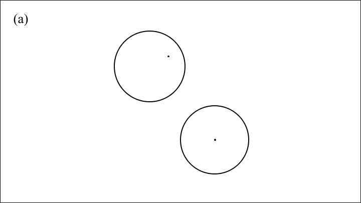
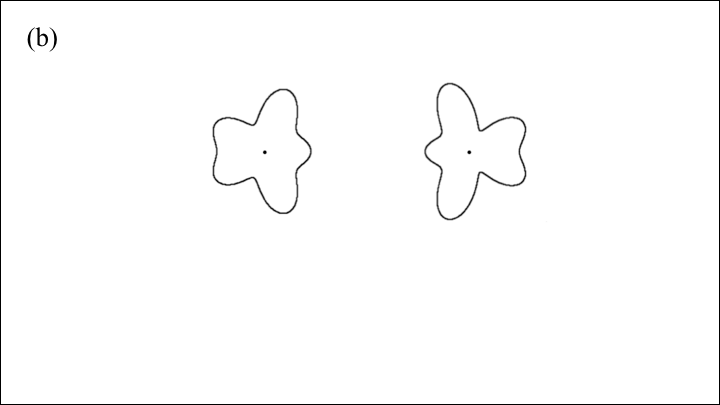
Figure 2: Stimuli used in (a) the dot position reproduction task and (b) the shape reproduction task.

Experiment 1(b)

Experiment 1(b) had some trials in which either the horizontal coordinate or the vertical coordinate of the reference dot was 0 px. In each trial the two parameters of the reference dot were generated from [20 px, 80 px] $\times$ [20 px, 80 px], 0 px $\times$ [20 px, 80 px], or [20 px, 80 px] $\times$ 0 px with probabilities .5, .25, and .25 respectively. The trials generated from [20 px, 80 px] $\times$ [20 px, 80 px] were double-channel trials and the trials generated from 0 px $\times$ [20 px, 80 px] and [20 px, 80 px] $\times$ 0 px were single-channel trials. There were 1680 trials in total divided equally in eight sessions. In all the other aspects, Experiment 1(b) was identical to 1(a).

Experiment 1(c)

There were eight sessions, each including 210 trials. The first four sessions contained double-channel trials only and the four sessions ran later contained single-channel trials only. The two parameters of reference stimulus in the double-channel sessions were randomly generated from [20 px, 80 px] $\times$ [20 px, 80 px] in each trial. The two parameters of reference stimulus in the single-channel sessions were randomly generated from 0 px $\times$ [20 px, 80 px] or [20 px, 80 px] $\times$ 0 px. In all the other aspects, Experiment 1(c) was identical to 1(b).

Experiment 2

Experiment 2 was a floral shape reproduction task. Examples of two floral shapes together with their centers are shown in Figure 2(b). Two such configurations were presented simultaneously in each trial. The reference stimulus was on the left and it was fixed. The test stimulus was on the right and it was modifiable. Both shapes were generated from this function:

$$X =\mathrm{cos}(.02\pi\triangle)[70+\alpha\mathrm{cos}(.06\pi\triangle)+\beta\mathrm{cos}(.1\pi\triangle)],$$ (8)

$$Y =\mathrm{sin}(.02\pi\triangle)[70+\alpha\mathrm{cos}(.06\pi\triangle)+\beta\mathrm{cos}(.1\pi\triangle)],$$

where $X$ and $Y$ are the horizontal coordinate (px) and vertical coordinate (px) of the shape. $\triangle$ spans all the integers from 0 to 99. $\alpha$ and $\beta$ in the function are amplitude 1 and amplitude 2 that determine the exact configuration of the floral shape.

We used $\alpha$ and $\beta$ to denote the amplitudes for the reference shape. For the modifiable test shape, we replaced $\alpha$ with $A$ and $\beta$ with $B$. In other words, $A$ was represented as amplitude 1 and $B$ as amplitude 2 for the modifiable shape. The amplitudes of the modifiable shape were initially selected from the interval [-35 px, 35 px]. The participants were asked to match the reference shape by modifying the test one. Since the computer program can only read the horizontal move and the vertical move of the trackball, a transformation function from the trackball move to the amplitude move was imposed:

$$A_{new} =A+\frac{\mathrm{sign}(\triangle x)}{100}(70-A-|B|),$$ (9)

$$B_{new} =B+\frac{\mathrm{sign}(\triangle y)}{100}(70-|A|-B).$$

Here $\triangle x$ is the horizontal move of the trackball and $\triangle y$ is the vertical move of the trackball. $\triangle x$ and $\triangle y$ can be updated every 1 px or -1 px. In each trial, the program recorded amplitude 1 and amplitude 2 of the reference shape and the finalized test shape. The RT in each trial was recorded.

Experiment 2 contained three designs: 2(a), 2(b), and 2(c). All the trials in Experiment 2 were double-channel trials. The significant differences among them were: Experiments 2(b) and 2(c) tracked the change of amplitudes of the test shape every 10 ms within each trial while Experiment 2(a) did not include that function. Experiment 2(c) and Experiment 2(b) were almost identical. Experiment 2(c) was ran to examine if the results obtained from Experiment 2(b) at Purdue can be replicated at NCKU.

Experiment 2(a)

For each fixed reference shape, amplitude 1 ($\alpha$) was randomly selected from an interval [-30 px, 30 px] and amplitude 2 ($\beta$) was selected from the same interval. We ran 1890 trials for each participant divided equally in nine sessions.

Experiment 2(b)

This experiment was identical to Experiment 2(a) except the program recorded the amplitudes of the test shape that was being modified every 10 ms in each trial.

Experiment 2(c)

This experiment contained four sessions, each containing 10 practice trials and 200 main trials. In all the other aspects, it was identical to Experiment 2(b).

Results

There were two parameters defined the reference stimulus (denoted as $\alpha$ and $\beta$ ) and two parameters defined the test stimulus (denoted as $A$ and $B$). Table 3 presents what these parameters stand for. We expected in both experiments, the subjects implemented the parallel AND, serial AND, or coactive manner to adjust $A$ and $B$. The stopping rule OR should not be used as in the experiments both features ($A$ and $B$) of the test stimulus had to match the features ($\alpha$ and $\beta$ ) of the reference stimulus.

Table 3: Parameters $(\alpha,\beta)$ of the reference stimuli and parameters $(A,B)$ of the test stimuli.

Task	$\alpha$	$\beta$	$A$	$B$
Dot position	Horizontal	Vertical	Horizontal	Vertical
reproduction	coordinate	coordinate	coordinate of	coordinate of
	of the	of the	the test	the test
	reference dot	reference dot	dot	dot
Floral shape	Amplitude 1	Amplitude 2	Amplitude 1	Amplitude 2
reproduction	of the	of the	of the	of the
	reference shape	reference shape	test	test
			shape	shape

Dot Position Reproduction Task

Trackball Movements

Figure 7 shows the trackball movements in a typical trial in the dot position reproduction task. The trajectory of the trackball movements confirmed the third assumption of SFT that the subject adheres a single type of mental architecture from trial to trial. The red dot represents the location of the fixed reference dot. The test dot (blue) started from (0 px, 0 px) and after a sequence of movements for the horizontal coordinate and the vertical coordinate, the final location was very close to the target location indicating the coordinates were not adjusted in the parallel OR or serial OR or serial AND manner: If the stopping rule OR was used, one should expect the final location of the test dot aligned well with the target either horizontally or vertically but not both. If serial AND was used in the task, the two coordinates should not move simultaneously as observed in Figure 7. The trajectory implies parallel AND or coactive were used by the subjects in the task. However the trajectory is not able to differentiate parallel AND from coactive.

Figure 3: Trackball movements in a typical trial in the dot position reproduction task (plotted every 50ms).

Testing Selective Influence

Selective influence of $\alpha$ and $\beta$ on $T_{\alpha}$ and $T_{\beta}$ has ideally to be tested before SFT is implemented. In our experimental paradigm, channel $\alpha$ and channel $\beta$ were characterized by two properties. One was the physical parameters of the response, i.e., $A$ and $B$, and the other was the durations for the channels, i.e., $T_{\alpha}$ and $T_{\beta}$. We speculated that $(A,B)\looparrowleft(\alpha,\beta)$ is a sufficient (and perhaps also necessary) condition for $(T_{\alpha},T_{\beta})\looparrowleft(\alpha,\beta)$. If this speculation is accepted, we can test $(T_{\alpha},T_{\beta})\looparrowleft(\alpha,\beta)$ by inspecting whether $(A,B)\looparrowleft(\alpha,\beta)$. Please be aware we used the finalized coordinates of $A$ and $B$ rather than the intermediate coordinates while the dot was being moved for the test of $(A,B)\looparrowleft(\alpha,\beta)$.

The outliers of $A$ and $B$ were handled in this way: We computed $A-\alpha$ and $B-\beta$ for each trial. Any trial that was out of 3 standard deviations of the set of $A-\alpha$ or $B-\beta$ was considered as an outlier and was removed from further analysis. In order to test selective influence and implement SFT, both $\alpha$ and $\beta$ should have discrete levels. A two by two factorial design can be achieved in Experiment 1 if one splits $\alpha$ and $\beta$ with respect to 50 px. Of course other values can be chosen to make the discretization. Here we use 50 px as an example. We label interval [20 px, 50 px) one level and [50 px, 80 px] another. Table 4 presents the corresponding means and standard deviations of $A$ and $B$ conditional on different combinations of $\alpha$ and $\beta$ for Experiment 1.

Table 4: Means and standard deviations of the finalized horizontal coordinates and the finalized vertical coordinates of the test dots for Experiment 1.

Exp.	Subject	$([20\,\mathrm{px},50\,\mathrm{px}),[20\,\mathrm{px},50\,\mathrm{px}))$, $([20\,\mathrm{px},50\,\mathrm{px}),[50\,\mathrm{px},80\,\mathrm{px}])$, $([50\,\mathrm{px},80\,\mathrm{px}],[20\,\mathrm{px},50\,\mathrm{px}))$, $([50\,\mathrm{px},80\,\mathrm{px}],[50\,\mathrm{px},80\,\mathrm{px}])$
1(a)	S1	$(37.10\pm 9.06,33.81\pm 9.44)$, $(37.68\pm 9.78,61.59\pm 9.32)$, $(66.57\pm 9.78,33.88\pm 9.32)$, $(66.56\pm 8.05,63.03\pm 9.35)$
1(a)	S2	$(34.85\pm 9.75,31.03\pm 10.25)$, $(34.41\pm 10.34,61.37\pm 10.15)$, $(62.84\pm 10.68,33.17\pm 10.94)$, $(62.79\pm 10.20,64.16\pm 10.55)$
1(a)	S3	$(42.30\pm 11.65,36.10\pm 10.78)$, $(38.09\pm 10.89,68.75\pm 10.07)$, $(75.01\pm 9.13,33.84\pm 8.55)$, $(72.41\pm 10.21,63.07\pm 11.24)$
1(b)	S7	$(37.55\pm 13.02,34.98\pm 14.28)$, $(35.18\pm 11.35,64.02\pm 10.11)$, $(66.02\pm 10.43,34.95\pm 11.74)$, $(66.85\pm 10.79,61.89\pm 10.07)$
1(b)	S8	$(30.58\pm 12.54,44.69\pm 13.09)$, $(25.25\pm 11.97,68.99\pm 11.63)$, $(59.54\pm 11.24,38.93\pm 14.41)$, $(52.03\pm 12.16,69.30\pm 12.30)$
1(b)	S9	$(32.58\pm 12.03,39.93\pm 12.32)$, $(30.85\pm 11.89,66.42\pm 10.22)$, $(61.21\pm 11.53,40.29\pm 11.78)$, $(56.99\pm 11.44,64.92\pm 11.81)$
1(b)	S10	$(31.58\pm 9.89,43.92\pm 11.55)$, $(31.03\pm 9.24,66.72\pm 8.30)$, $(57.93\pm 9.17,42.23\pm 11.41)$, $(58.41\pm 9.87,67.01\pm 9.38)$
1(b)	S11	$(33.77\pm 13.87,32.83\pm 13.96)$, $(34.71\pm 14.18,63.51\pm 11.72)$, $(66.49\pm 10.62,26.71\pm 13.05)$, $(67.32\pm 10.76,60.70\pm 11.16)$
1(c)	S12	$(39.43\pm 14.16,42.44\pm 12.86)$, $(32.80\pm 12.29,71.77\pm 11.35)$, $(68.43\pm 9.90,35.12\pm 13.31)$, $(60.75\pm 11.11,67.63\pm 12.69)$
1(c)	S13	$(37.07\pm 7.79,39.52\pm 8.96)$, $(35.59\pm 9.67,62.94\pm 10.86)$, $(58.81\pm 8.06,39.13\pm 10.27)$, $(61.04\pm 9.04,65.60\pm 10.75)$
1(c)	S14	$(40.20\pm 10.03,36.52\pm 11.65)$, $(38.82\pm 10.43,61.83\pm 10.94)$, $(64.83\pm 9.37,35.00\pm 10.45)$, $(66.54\pm 9.77,61.38\pm 8.17)$
1(c)	S15	$(42.43\pm 10.26,46.76\pm 9.87)$, $(38.66\pm 10.08,73.33\pm 11.93)$, $(69.78\pm 10.47,44.11\pm 8.95)$, $(67.53\pm 9.37,69.77\pm 9.94)$
1(c)	S16	$(42.76\pm 8.99,43.38\pm 10.01)$, $(39.62\pm 10.17,68.13\pm 9.98)$, $(65.96\pm 8.71,42.22\pm 10.37)$, $(64.06\pm 9.46,67.65\pm 9.95)$

We then conducted four two sample Kolmogorov–Smirnov(KS) tests for each subject to examine marginal selectivity (4): $T_{\alpha_{i}}$ and $T_{\beta_{j}}$ were replaced with $A_{i}$ and $B_{j}$ that stand for the coordinates of the test dot conditional on the reference dot $\alpha_{i}\beta_{j},i,j\in\left\{1,2\right\}$. Table 5 presents the statistics for the tests. Each column of numbers represents a particular paired comparison for the subjects. For instance, $([20\,\mathrm{px},50\,\mathrm{px}),)$ compared the $A\mathrm{s}$ across different levels of $\beta$ but fixed $\alpha=[20\,\mathrm{px},50\,\mathrm{px})$. $(,[50\,\mathrm{px},80\,\mathrm{px}])$ compared the $B\mathrm{s}$ across different levels of $\alpha$ but fixed $\beta=[50\,\mathrm{px},80\,\mathrm{px}]$. We conclude that marginal selectivity was confirmed for S1, S7, S10, S13, and S14 ($\mathrm{alpha}=.05/4$ for the Bonferroni adjustment).

Table 5: Two sample KS tests for marginal selectivity for Experiment 1.

Exp.	Subject	$([20\,\mathrm{px},50\,\mathrm{px}),)$	$([50\,\mathrm{px},80\,\mathrm{px}],)$	$(,[20\,\mathrm{px},50\,\mathrm{px}))$	$(,[50\,\mathrm{px},80\,\mathrm{px}])$	Marginal
						selectivity?
1(a)	S1	.046(.697)	.061(.397)	.048(.672)	.066(.272)	Yes
1(a)	S2	.050(.616)	.055(.514)	.102(.017)	.107(.011)	No
1(a)	S3	.156(.000)	.122(.003)	.125(.002)	.275(.000)	No
1(b)	S7	.138(.049)	.067(.756)	.070(.696)	.106(.230)	Yes
1(b)	S8	.189(.001)	.306(.000)	.180(.002)	.058(.927)	No
1(b)	S9	.095(.304)	.196(.001)	.078(.546)	.145(.037)	No
1(b)	S10	.081(.467)	.051(.980)	.099(.310)	.057(.917)	Yes
1(b)	S11	.196(.001)	.099(.274)	.076(.608)	.058(.892)	No
1(c)	S12	.252(.000)	.326(.000)	.215(.000)	.200(.001)	No
1(c)	S13	.140(.037)	.140(.038)	.077(.550)	.143(.039)	Yes
1(c)	S14	.100(.299)	.139(.038)	.090(.361)	.103(.276)	Yes
1(c)	S15	.182(.002)	.131(.073)	.171(.007)	.199(.001)	No
1(c)	S16	.187(.002)	.110(.168)	.079(.524)	.063(.840)	No

Note: Each number outside of the brackets is the KS statistic value and each number in the brackets is the $p$ value.

For those who passed the test of marginal selectivity, we investigated if selective influence secured by conducting LFT. LFT is applicable only if $A$ and $B$ are discrete. One can choose any value to create two levels for $A$ and $B$ or discretize $A$ and $B$ into multiple levels. For example, we created two levels for $A$: {smaller than or equal to 50 px, larger than 50 px}, labeled as $\left\{a_{1},a_{2}\right\}$, and two levels for $B$: {smaller than or equal to 50 px, larger than 50 px}, labeled as $\left\{b_{1},b_{2}\right\}$. The numbers in the cells of Table 6 are the joint probabilities for the discretized $(A_{ij},\>B_{ij}),i,j\in\left\{1,2\right\}$ and the numbers outside are the marginal probabilities.

Table 6: Joint distributions for the discretized $(A_{ij},\>B_{ij}),i,j\in\left\{1,2\right\}$ for S1, S7, S10, S13, and S14. S1 participated in Experiment 1(a). S7 and S10 participated in Experiment 1(b). S13 and S14 participated in Experiment 1(c).

S1
$([20\,\mathrm{px},50\,\mathrm{px}),$	$B=b_{1}$	$B=b_{2}$		$([20\,\mathrm{px},50\,\mathrm{px}),$	$B=b_{1}$	$B=b_{2}$
$[20\,\mathrm{px},50\,\mathrm{px}))$				$[50\,\mathrm{px},80\,\mathrm{px}])$
$A=a_{1}$	.8811	.0419	.9230	$A=a_{1}$	.1361	.7711	.9072
$A=a_{2}$	.0749	.0022	.0771	$A=a_{2}$	.0173	.0756	.0928
	.9560	.0441			.1534	.8467
$([50\,\mathrm{px},80\,\mathrm{px}],$	$B=b_{1}$	$B=b_{2}$		$([50\,\mathrm{px},80\,\mathrm{px}],$	$B=b_{1}$	$B=b_{2}$
$[20\,\mathrm{px},50\,\mathrm{px}))$				$[50\,\mathrm{px},80\,\mathrm{px}])$
$A=a_{1}$	.0590	.0024	.0614	$A=a_{1}$	.0069	.0161	.0230
$A=a_{2}$	.9127	.0259	.9386	$A=a_{2}$	.1034	.8736	.9770
	.9717	.0283			.1103	.8897

S7
$([20\,\mathrm{px},50\,\mathrm{px}),$	$B=b_{1}$	$B=b_{2}$		$([20\,\mathrm{px},50\,\mathrm{px}),$	$B=b_{1}$	$B=b_{2}$
$[20\,\mathrm{px},50\,\mathrm{px}))$				$[50\,\mathrm{px},80\,\mathrm{px}])$
$A=a_{1}$	.7122	.1220	.8342	$A=a_{1}$	.0904	.8079	.8983
$A=a_{2}$	.1610	.0049	.1659	$A=a_{2}$	.0113	.0904	.1017
	.8732	.1269			.1017	.8983
$([50\,\mathrm{px},80\,\mathrm{px}],$	$B=b_{1}$	$B=b_{2}$		$([50\,\mathrm{px},80\,\mathrm{px}],$	$B=b_{1}$	$B=b_{2}$
$[20\,\mathrm{px},50\,\mathrm{px}))$				$[50\,\mathrm{px},80\,\mathrm{px}])$
$A=a_{1}$	.0769	.0103	.0872	$A=a_{1}$	.015	.06	.075
$A=a_{2}$	.8308	.0820	.9128	$A=a_{2}$	.135	.79	.927
	.9077	.0923			.150	.85

S10
$([20\,\mathrm{px},50\,\mathrm{px}),$	$B=b_{1}$	$B=b_{2}$		$([20\,\mathrm{px},50\,\mathrm{px}),$	$B=b_{1}$	$B=b_{2}$
$[20\,\mathrm{px},50\,\mathrm{px}))$				$[50\,\mathrm{px},80\,\mathrm{px}])$
$A=a_{1}$	.6866	.2935	.9801	$A=a_{1}$	.0223	.9688	.9911
$A=a_{2}$	.0199	0	.0199	$A=a_{2}$	0	.0089	.0089
	.7065	.2935			.0223	.9777
$([50\,\mathrm{px},80\,\mathrm{px}],$	$B=b_{1}$	$B=b_{2}$		$([50\,\mathrm{px},80\,\mathrm{px}],$	$B=b_{1}$	$B=b_{2}$
$[20\,\mathrm{px},50\,\mathrm{px}))$				$[50\,\mathrm{px},80\,\mathrm{px}])$
$A=a_{1}$	.1618	.0636	.2254	$A=a_{1}$	.0126	.2075	.2201
$A=a_{2}$	.5780	.1965	.7745	$A=a_{2}$	.0503	.7296	.7799
	.7398	.2601			.0629	.9371

S13
$([20\,\mathrm{px},50\,\mathrm{px}),$	$B=b_{1}$	$B=b_{2}$		$([20\,\mathrm{px},50\,\mathrm{px}),$	$B=b_{1}$	$B=b_{2}$
$[20\,\mathrm{px},50\,\mathrm{px}))$				$[50\,\mathrm{px},80\,\mathrm{px}])$
$A=a_{1}$	.8357	.1063	.9420	$A=a_{1}$	.1105	.8368	.9473
$A=a_{2}$	.0531	.0048	.0579	$A=a_{2}$	.0211	.0316	.0527
	.8888	.1111			.1316	.8684
$([50\,\mathrm{px},80\,\mathrm{px}],$	$B=b_{1}$	$B=b_{2}$		$([50\,\mathrm{px},80\,\mathrm{px}],$	$B=b_{1}$	$B=b_{2}$
$[20\,\mathrm{px},50\,\mathrm{px}))$				$[50\,\mathrm{px},80\,\mathrm{px}])$
$A=a_{1}$	.1014	.0242	.1256	$A=a_{1}$	.0107	.1123	.1230
$A=a_{2}$	.7488	.1256	.8744	$A=a_{2}$	.0963	.7807	.8770
	.8502	.1498			.1070	.8930

Table 6: Joint distributions for the discretized $(A_{ij},\>B_{ij}),i,j\in\left\{1,2\right\}$ for S1, S7, S10, S13, and S14 (continued). S1 participated in Experiment 1(a). S7 and S10 participated in Experiment 1(b). S13 and S14 participated in Experiment 1(c).

S14
$([20\,\mathrm{px},50\,\mathrm{px}),$	$B=b_{1}$	$B=b_{2}$		$([20\,\mathrm{px},50\,\mathrm{px}),$	$B=b_{1}$	$B=b_{2}$
$[20\,\mathrm{px},50\,\mathrm{px}))$				$[50\,\mathrm{px},80\,\mathrm{px}])$
$A=a_{1}$	.7104	.1257	.8361	$A=a_{1}$	.1064	.7394	.8458
$A=a_{2}$	.1530	.0109	.1639	$A=a_{2}$	.0426	.1117	.1543
	.8634	.1366			.1490	.8511
$([50\,\mathrm{px},80\,\mathrm{px}],$	$B=b_{1}$	$B=b_{2}$		$([50\,\mathrm{px},80\,\mathrm{px}],$	$B=b_{1}$	$B=b_{2}$
$[20\,\mathrm{px},50\,\mathrm{px}))$				$[50\,\mathrm{px},80\,\mathrm{px}])$
$A=a_{1}$	.0593	.0085	.0678	$A=a_{1}$	0	.0511	.0511
$A=a_{2}$	.8517	.0805	.9322	$A=a_{2}$	.1080	.8409	.9489
	.9110	.0890			.1080	.8920

We observe the marginal probabilities not exactly equal across conditions, for instance

$$\mathrm{Pr}(A =a_{1})\mid_{([20\,\mathrm{px},50\,\mathrm{px}),[20\,\mathrm{px},50\,\mathrm{px}))}=.9230\neq\mathrm{Pr}(A=a_{1})\mid_{([20\,\mathrm{px},50\,\mathrm{px}),[50\,\mathrm{px},80\,\mathrm{px}])}=.9072,$$

$$\mathrm{Pr}(A =a_{1})\mid_{([50\,\mathrm{px},80\,\mathrm{px}],[20\,\mathrm{px},50\,\mathrm{px}))}=.0614\neq\mathrm{Pr}(A=a_{1})\mid_{([50\,\mathrm{px},80\,\mathrm{px}],[50\,\mathrm{px},80\,\mathrm{px}])}=.0230,$$

$$\mathrm{Pr}(B =b_{1})\mid_{([20\,\mathrm{px},50\,\mathrm{px}),[20\,\mathrm{px},50\,\mathrm{px}))}=.9560\neq\mathrm{Pr}(B=b_{1})\mid_{([50\,\mathrm{px},80\,\mathrm{px}],[20\,\mathrm{px},50\,\mathrm{px}))}=.9717,$$

$$\mathrm{Pr}(B =b_{1})\mid_{([20\,\mathrm{px},50\,\mathrm{px}),[50\,\mathrm{px},80\,\mathrm{px}])}=.1534\neq\mathrm{Pr}(B=b_{1})\mid_{([50\,\mathrm{px},80\,\mathrm{px}],[50\,\mathrm{px},80\,\mathrm{px}])}=.1103,$$

for S1. We considered .9230 and .9072, .0614 and .0230, .9560 and .9717, and .1534 and .1103 statistically equal as marginal selectivity was established statistically for that subject (Table 5).

In order to implement LFT, one requirement is (4) has to be strictly hold. In order to fulfill this requirement, we forced

$$\mathrm{Pr}(A =a_{1})\mid_{([20\,\mathrm{px},50\,\mathrm{px}),[20\,\mathrm{px},50\,\mathrm{px}))}=\mathrm{Pr}(A=a_{1})\mid_{([20\,\mathrm{px},50\,\mathrm{px}),[50\,\mathrm{px},80\,\mathrm{px}])}=(.9230+.9072)/2=.9151,$$

$$\mathrm{Pr}(A =a_{2})\mid_{([20\,\mathrm{px},50\,\mathrm{px}),[20\,\mathrm{px},50\,\mathrm{px}))}=\mathrm{Pr}(A=a_{2})\mid_{([20\,\mathrm{px},50\,\mathrm{px}),[50\,\mathrm{px},80\,\mathrm{px}])}=(.0771+.0928)/2=.0849,$$

$$\mathrm{Pr}(B =b_{1})\mid_{([20\,\mathrm{px},50\,\mathrm{px}),[20\,\mathrm{px},50\,\mathrm{px}))}=\mathrm{Pr}(B=b_{1})\mid_{([50\,\mathrm{px},80\,\mathrm{px}],[20\,\mathrm{px},50\,\mathrm{px}))}=(.9560+.9717)/2=.9638,$$

$$\mathrm{Pr}(B =b_{2})\mid_{([20\,\mathrm{px},50\,\mathrm{px}),[20\,\mathrm{px},50\,\mathrm{px}))}=\mathrm{Pr}(B=b_{2})\mid_{([50\,\mathrm{px},80\,\mathrm{px}],[20\,\mathrm{px},50\,\mathrm{px}))}=(.0441+.0283)/2=.0362,$$

and averaged the other marginal probability pairs in the same way. The joint probabilities in the cells of Table 6 were modified by keeping the value of $\mathrm{Pr}(A=a_{1},B=b_{1})$ for each stimulus and changing values for $P(A=a_{1},B=b_{2})$, $P(A=a_{2},B=b_{1})$, and $P(A=a_{2},B=b_{2})$ according to the change of the corresponding marginal probabilities. For instance, for S1 for stimulus $([20\,\mathrm{px},50\,\mathrm{px}),[20\,\mathrm{px},50\,\mathrm{px}))$, the modified joint probabilities are

$$\mathrm{Pr}(A =a_{1},B=b_{1})=.8811,$$

$$\mathrm{Pr}(A =a_{1},B=b_{2})=.9151-.8811=.0340,$$

$$\mathrm{Pr}(A =a_{2},B=b_{1})=.9638-.8811=.0827,$$

$$\mathrm{Pr}(A =a_{2},B=b_{2})=.0849-.0827=.0022.$$

LFT was passed as we were able to find nonnegative solutions for LFT (Table 7). It indicates selective influence of $\alpha$ and $\beta$ on $A$ and $B$ was established for these subjects. We found LFT passed for all the other ways of discretization that we tried for $A$ and $B$. We then considered $(T_{\alpha},T_{\beta})\looparrowleft(\alpha,\beta)$ was successfully established for S1, S7, S10, S13, and S14.

Table 7: Solutions for LFT for S1, S7, S10, S13, and S14 in Experiment 1. S1 participated in Experiment 1(a). S7 and S10 participated in Experiment 1(b). S13 and S14 participated in Experiment 1(c).

Subject	$(Q_{a_{1}a_{1}b_{1}b_{1}},\,Q_{a_{1}a_{1}b_{1}b_{2}},\,\ldots,\,Q_{a_{2}a_{2}b_{2}b_{2}})^{T}$
S1	$(.0069,0,0,0,.0909,.7833,.034,0,0,.0353,0,0,0,.0474,0,.0022)^{T}$
S7	$(0,0,0,.0041,0,.7616,.0904,.0101,.015,.0619,0,0,.0204,.0365,0,0)^{T}$
S10	$(.0126,.1348,0,.0609,0,.5614,.03,.1859,0,.0144,0,0,0,0,0,0)^{T}$
S13	$(.0019,.0657,0,.0013,.001,.7671,.1076,0,0,.0338,.0088,.0128,0,0,0,0)^{T}$
S14	$(0,0,0,.0001,0,.7281,.1064,.0063,0,.0593,0,0,.0221,.0777,0,0)^{T}$

Testing Stochastic Dominance

For each participant, we considered the trial with RT outside of 5 standard deviations of the entire set of RTs an outlier and it was not included in the further analysis. In the earlier part of this article, we created two levels for $\alpha$ and $\beta$, [20 px, 50 px) one level and [50 px, 80 px] another. In order to test stochastic dominance, what exactly level 1 and level 2 $\alpha$ and $\beta$ stand for should be identified. We observed some subjects spent more time when the target location was far from the center of the circle and others spent more time to move to a location closer to the center as they had to be more careful with their action. The exact assignment of level 1 and level 2 for each subject can be found in Table 8. The assignment was based on the observation of the dataset. The interval range that was processed more slowly was labeled level one and the other range was labeled level two.

Table 8: The assignment of level 1 and level 2 for Experiment 1.

Experiment	Level 1: $[20\,\mathrm{px},\,50\,\mathrm{px})$	Level 1: $[50\,\mathrm{px},\,80\,\mathrm{px}]$
	Level 2: $[50\,\mathrm{px},\,80\,\mathrm{px}]$	Level 2: $[20\,\mathrm{px},\,50\,\mathrm{px})$
1(a)	S1, S2, S3
1(b)		S7, S8, S9, S10, S11
1(c)	S12, S14, S15, S16	S13

The left column of Figure 4 presents the survival functions of RT for the subjects who passed the test of selective influence. In order to test if those survival functions satisfy stochastic dominance (5), two one tail KS tests were performed on each of the four paired variables. For instance, in order to test the first inequality in (5), we required the maximum of $S_{\alpha_{1}\beta_{1}}(t)-S_{\alpha_{1}\beta_{2}}(t)$ larger than or equal to 0 and the maximum of $S_{\alpha_{1}\beta_{2}}(t)-S_{\alpha_{1}\beta_{1}}(t)$ equal to zero. The statistical results (Table 9) support the assumption of stochastic dominance for subject S1, S7, S10, S13, and S14 with the assignment presented in Table 8 as for each subject the $p$ values in the bottom row were larger than the critical value $\mathrm{alpha}=.05/4$. Note for S13 and S14, the four survival functions of RT were not statistically different from each other.

The left column of Figure 6 presents the survival functions of RT for those subjects who did not pass the test of selective influence. They also passed the test of stochastic dominance ($\mathrm{alpha}=.05/4$, Table 10). Note that for subject S8, S15, and S16, the four survival functions of RT were not statistically different from each other.

Table 9: $p$ values of the one tail KS tests for stochastic dominance for S1, S7, S10, S13, and S14 in Experiment 1. S1 participated in Experiment 1(a). S7 and S10 participated in Experiment 1(b). S13 and S14 participated in Experiment 1(c).

S1
$S_{\alpha_{1}\beta_{1}}>S_{\alpha_{1}\beta_{2}}$	$S_{\alpha_{1}\beta_{1}}>S_{\alpha_{2}\beta_{1}}$	$S_{\alpha_{1}\beta_{2}}>S_{\alpha_{2}\beta_{2}}$	$S_{\alpha_{2}\beta_{1}}>S_{\alpha_{2}\beta_{2}}$
.075(.077)	.047(.379)	.098(.014)	.113(.004)
$S_{\alpha_{1}\beta_{1}}<S_{\alpha_{1}\beta_{2}}$	$S_{\alpha_{1}\beta_{1}}<S_{\alpha_{2}\beta_{1}}$	$S_{\alpha_{1}\beta_{2}}<S_{\alpha_{2}\beta_{2}}$	$S_{\alpha_{2}\beta_{1}}<S_{\alpha_{2}\beta_{2}}$
.048(.344)	.038(.531)	.007(.977)	.005(.990)
S7
$S_{\alpha_{1}\beta_{1}}>S_{\alpha_{1}\beta_{2}}$	$S_{\alpha_{1}\beta_{1}}>S_{\alpha_{2}\beta_{1}}$	$S_{\alpha_{1}\beta_{2}}>S_{\alpha_{2}\beta_{2}}$	$S_{\alpha_{2}\beta_{1}}>S_{\alpha_{2}\beta_{2}}$
.114(.076)	.132(.037)	.302(.000)	.289(.000)
$S_{\alpha_{1}\beta_{1}}<S_{\alpha_{1}\beta_{2}}$	$S_{\alpha_{1}\beta_{1}}<S_{\alpha_{2}\beta_{1}}$	$S_{\alpha_{1}\beta_{2}}<S_{\alpha_{2}\beta_{2}}$	$S_{\alpha_{2}\beta_{1}}<S_{\alpha_{2}\beta_{2}}$
.007(.989)	.006(.993)	.015(.958)	.015(.960)
S10
$S_{\alpha_{1}\beta_{1}}>S_{\alpha_{1}\beta_{2}}$	$S_{\alpha_{1}\beta_{1}}>S_{\alpha_{2}\beta_{1}}$	$S_{\alpha_{1}\beta_{2}}>S_{\alpha_{2}\beta_{2}}$	$S_{\alpha_{2}\beta_{1}}>S_{\alpha_{2}\beta_{2}}$
.086(.299)	.143(.022)	.181(.002)	.099(.128)
$S_{\alpha_{1}\beta_{1}}<S_{\alpha_{1}\beta_{2}}$	$S_{\alpha_{1}\beta_{1}}<S_{\alpha_{2}\beta_{1}}$	$S_{\alpha_{1}\beta_{2}}<S_{\alpha_{2}\beta_{2}}$	$S_{\alpha_{2}\beta_{1}}<S_{\alpha_{2}\beta_{2}}$
.024(.907)	.004(.996)	.015(.958)	.019(.927)
S13
$S_{\alpha_{1}\beta_{1}}>S_{\alpha_{1}\beta_{2}}$	$S_{\alpha_{1}\beta_{1}}>S_{\alpha_{2}\beta_{1}}$	$S_{\alpha_{1}\beta_{2}}>S_{\alpha_{2}\beta_{2}}$	$S_{\alpha_{2}\beta_{1}}>S_{\alpha_{2}\beta_{2}}$
.146(.015)	.062(.481)	.107(.094)	.139(.022)
$S_{\alpha_{1}\beta_{1}}<S_{\alpha_{1}\beta_{2}}$	$S_{\alpha_{1}\beta_{1}}<S_{\alpha_{2}\beta_{1}}$	$S_{\alpha_{1}\beta_{2}}<S_{\alpha_{2}\beta_{2}}$	$S_{\alpha_{2}\beta_{1}}<S_{\alpha_{2}\beta_{2}}$
.016(.951)	.036(.783)	.073(.334)	.004(.996)
S14
$S_{\alpha_{1}\beta_{1}}>S_{\alpha_{1}\beta_{2}}$	$S_{\alpha_{1}\beta_{1}}>S_{\alpha_{2}\beta_{1}}$	$S_{\alpha_{1}\beta_{2}}>S_{\alpha_{2}\beta_{2}}$	$S_{\alpha_{2}\beta_{1}}>S_{\alpha_{2}\beta_{2}}$
.041(.736)	.064(.430)	.105(.135)	.039(.732)
$S_{\alpha_{1}\beta_{1}}<S_{\alpha_{1}\beta_{2}}$	$S_{\alpha_{1}\beta_{1}}<S_{\alpha_{2}\beta_{1}}$	$S_{\alpha_{1}\beta_{2}}<S_{\alpha_{2}\beta_{2}}$	$S_{\alpha_{2}\beta_{1}}<S_{\alpha_{2}\beta_{2}}$
.095(.192)	.034(.795)	.012(.972)	.064(.439)

Note: Each number outside of the brackets is the KS statistic value and each number in the brackets is the $p$ value.

Table 10: One tail KS tests for stochastic dominance for S2, S3, S8, S9, S11, S12, S15, and S16 in Experiment 1. S2 and S3 participated in Experiment 1(a). S8, S9, and S11 participated in Experiment 1(b). S12, S15, and S16 participated in Experiment 1(c).

S2
$S_{\alpha_{1}\beta_{1}}>S_{\alpha_{1}\beta_{2}}$	$S_{\alpha_{1}\beta_{1}}>S_{\alpha_{2}\beta_{1}}$	$S_{\alpha_{1}\beta_{2}}>S_{\alpha_{2}\beta_{2}}$	$S_{\alpha_{2}\beta_{1}}>S_{\alpha_{2}\beta_{2}}$
.132(.000)	.065(.153)	.040(.493)	.086(.040)
$S_{\alpha_{1}\beta_{1}}<S_{\alpha_{1}\beta_{2}}$	$S_{\alpha_{1}\beta_{1}}<S_{\alpha_{2}\beta_{1}}$	$S_{\alpha_{1}\beta_{2}}<S_{\alpha_{2}\beta_{2}}$	$S_{\alpha_{2}\beta_{1}}<S_{\alpha_{2}\beta_{2}}$
.012(.936)	.026(.742)	.039(.513)	.023(.799)
S3
$S_{\alpha_{1}\beta_{1}}>S_{\alpha_{1}\beta_{2}}$	$S_{\alpha_{1}\beta_{1}}>S_{\alpha_{2}\beta_{1}}$	$S_{\alpha_{1}\beta_{2}}>S_{\alpha_{2}\beta_{2}}$	$S_{\alpha_{2}\beta_{1}}>S_{\alpha_{2}\beta_{2}}$
.160(.000)	.179(.000)	.052(.309)	.035(.595)
$S_{\alpha_{1}\beta_{1}}<S_{\alpha_{1}\beta_{2}}$	$S_{\alpha_{1}\beta_{1}}<S_{\alpha_{2}\beta_{1}}$	$S_{\alpha_{1}\beta_{2}}<S_{\alpha_{2}\beta_{2}}$	$S_{\alpha_{2}\beta_{1}}<S_{\alpha_{2}\beta_{2}}$
.000(1.000)	.000(1.000)	.038(.543)	.062(.190)
S8
$S_{\alpha_{1}\beta_{1}}>S_{\alpha_{1}\beta_{2}}$	$S_{\alpha_{1}\beta_{1}}>S_{\alpha_{2}\beta_{1}}$	$S_{\alpha_{1}\beta_{2}}>S_{\alpha_{2}\beta_{2}}$	$S_{\alpha_{2}\beta_{1}}>S_{\alpha_{2}\beta_{2}}$
.058(.561)	.082(.312)	.099(.137)	.087(.218)
$S_{\alpha_{1}\beta_{1}}<S_{\alpha_{1}\beta_{2}}$	$S_{\alpha_{1}\beta_{1}}<S_{\alpha_{2}\beta_{1}}$	$S_{\alpha_{1}\beta_{2}}<S_{\alpha_{2}\beta_{2}}$	$S_{\alpha_{2}\beta_{1}}<S_{\alpha_{2}\beta_{2}}$
.038(.786)	.062(.516)	.048(.628)	.024(.887)
S9
$S_{\alpha_{1}\beta_{1}}>S_{\alpha_{1}\beta_{2}}$	$S_{\alpha_{1}\beta_{1}}>S_{\alpha_{2}\beta_{1}}$	$S_{\alpha_{1}\beta_{2}}>S_{\alpha_{2}\beta_{2}}$	$S_{\alpha_{2}\beta_{1}}>S_{\alpha_{2}\beta_{2}}$
.041(.728)	.079(.315)	.163(.005)	.121(.053)
$S_{\alpha_{1}\beta_{1}}<S_{\alpha_{1}\beta_{2}}$	$S_{\alpha_{1}\beta_{1}}<S_{\alpha_{2}\beta_{1}}$	$S_{\alpha_{1}\beta_{2}}<S_{\alpha_{2}\beta_{2}}$	$S_{\alpha_{2}\beta_{1}}<S_{\alpha_{2}\beta_{2}}$
.091(.209)	.029(.858)	.015(.957)	.040(.728)
S11
$S_{\alpha_{1}\beta_{1}}>S_{\alpha_{1}\beta_{2}}$	$S_{\alpha_{1}\beta_{1}}>S_{\alpha_{2}\beta_{1}}$	$S_{\alpha_{1}\beta_{2}}>S_{\alpha_{2}\beta_{2}}$	$S_{\alpha_{2}\beta_{1}}>S_{\alpha_{2}\beta_{2}}$
.169(.004)	.128(.041)	.071(.374)	.142(.019)
$S_{\alpha_{1}\beta_{1}}<S_{\alpha_{1}\beta_{2}}$	$S_{\alpha_{1}\beta_{1}}<S_{\alpha_{2}\beta_{1}}$	$S_{\alpha_{1}\beta_{2}}<S_{\alpha_{2}\beta_{2}}$	$S_{\alpha_{2}\beta_{1}}<S_{\alpha_{2}\beta_{2}}$
.010(.980)	.021(.919)	.053(.580)	.028(.854)
S12
$S_{\alpha_{1}\beta_{1}}>S_{\alpha_{1}\beta_{2}}$	$S_{\alpha_{1}\beta_{1}}>S_{\alpha_{2}\beta_{1}}$	$S_{\alpha_{1}\beta_{2}}>S_{\alpha_{2}\beta_{2}}$	$S_{\alpha_{2}\beta_{1}}>S_{\alpha_{2}\beta_{2}}$
.148(.011)	.089(.191)	.080(.296)	.138(.025)
$S_{\alpha_{1}\beta_{1}}<S_{\alpha_{1}\beta_{2}}$	$S_{\alpha_{1}\beta_{1}}<S_{\alpha_{2}\beta_{1}}$	$S_{\alpha_{1}\beta_{2}}<S_{\alpha_{2}\beta_{2}}$	$S_{\alpha_{2}\beta_{1}}<S_{\alpha_{2}\beta_{2}}$
.025(.884)	.056(.521)	.051(.613)	.023(.899)
S15
$S_{\alpha_{1}\beta_{1}}>S_{\alpha_{1}\beta_{2}}$	$S_{\alpha_{1}\beta_{1}}>S_{\alpha_{2}\beta_{1}}$	$S_{\alpha_{1}\beta_{2}}>S_{\alpha_{2}\beta_{2}}$	$S_{\alpha_{2}\beta_{1}}>S_{\alpha_{2}\beta_{2}}$
.041(.715)	.062(.493)	.049(.621)	.050(.627)
$S_{\alpha_{1}\beta_{1}}<S_{\alpha_{1}\beta_{2}}$	$S_{\alpha_{1}\beta_{1}}<S_{\alpha_{2}\beta_{1}}$	$S_{\alpha_{1}\beta_{2}}<S_{\alpha_{2}\beta_{2}}$	$S_{\alpha_{2}\beta_{1}}<S_{\alpha_{2}\beta_{2}}$
.104(.120)	.097(.174)	.032(.816)	.044(.699)
S16
$S_{\alpha_{1}\beta_{1}}>S_{\alpha_{1}\beta_{2}}$	$S_{\alpha_{1}\beta_{1}}>S_{\alpha_{2}\beta_{1}}$	$S_{\alpha_{1}\beta_{2}}>S_{\alpha_{2}\beta_{2}}$	$S_{\alpha_{2}\beta_{1}}>S_{\alpha_{2}\beta_{2}}$
.124(.048)	.131(.028)	.136(.030)	.139(.022)
$S_{\alpha_{1}\beta_{1}}<S_{\alpha_{1}\beta_{2}}$	$S_{\alpha_{1}\beta_{1}}<S_{\alpha_{2}\beta_{1}}$	$S_{\alpha_{1}\beta_{2}}<S_{\alpha_{2}\beta_{2}}$	$S_{\alpha_{2}\beta_{1}}<S_{\alpha_{2}\beta_{2}}$
.001(1.000)	.000(1.000)	.005(.995)	.034(.800)

Note: Each number outside of the brackets is the KS statistic value and each number in the brackets is the $p$ value.

Diagnosing Architectures According to SIC and MIC in the Presence of $(A,B)\looparrowleft(\alpha,\beta)$ and Stochastic Dominance

With the confirmation of ordering of the RT distributions, selective influence, and subject’s adherence to a single type of mental architecture, we then diagnosed how the horizontal and vertical coordinates of the test dot were adjusted by investigating the behavior of SIC and MIC for subject S1, S7, S10, S13, and S14. The SIC curves for these subjects are displayed in the right column of Figure 4. We implemented the R package developed by Houpt, Blaha, McIntire, Havig, and Townsend (2014) to inspect the statistical significance of SIC and MIC. Table 11 includes the statistics for SIC and MIC and the inferred architectures from SFT. $D^{+}$ is the most positive point of SIC and $D^{-}$ is the most negative point of SIC. We chose $\mathrm{alpha}=.33$ not the conventional critical value .05 here (Fox & Houpt, 2016) as the null hypothesis is SIC = 0 for all values of RT and MIC = 0 and hence conservative alpha levels bias the tests toward indicating a serial OR signature (flat SIC and zero MIC).

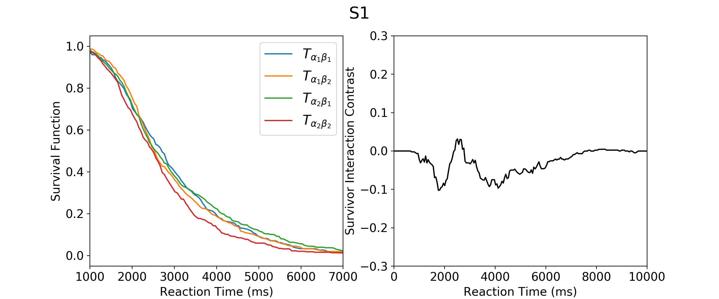
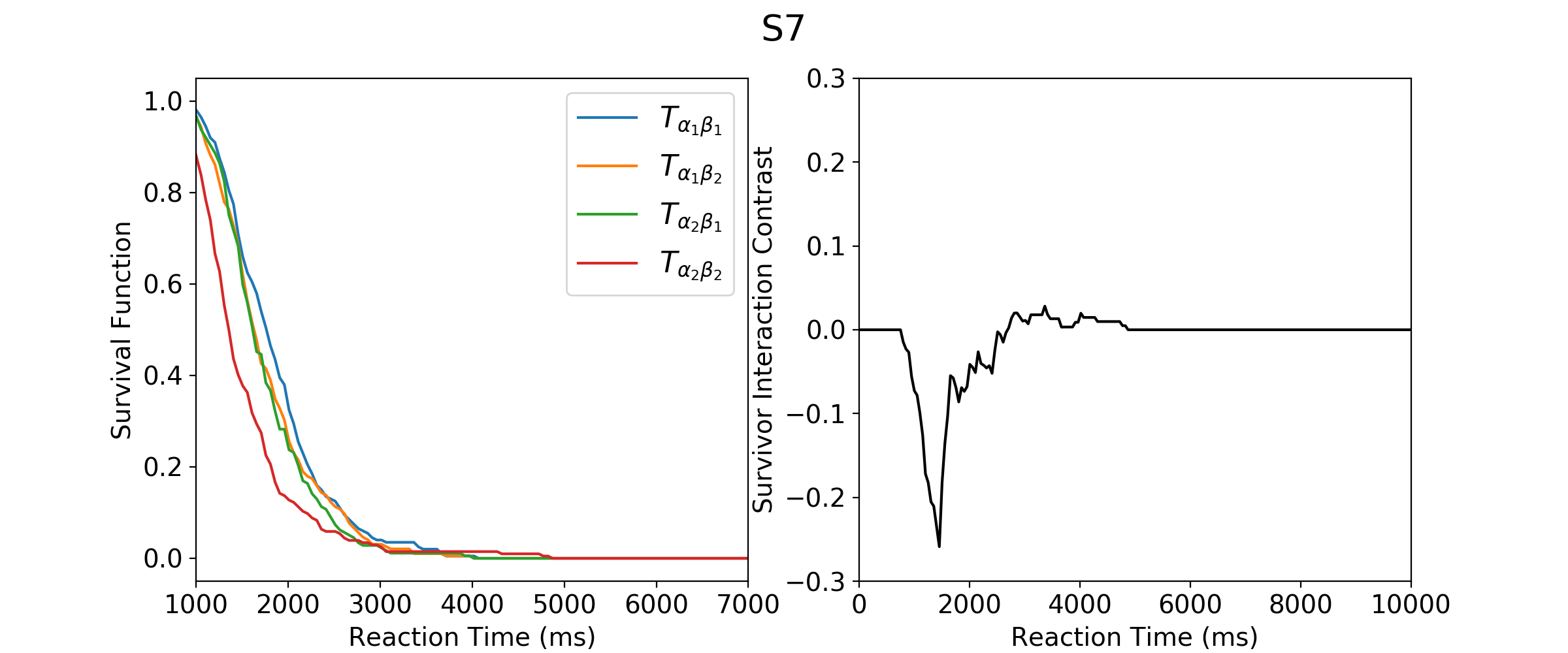
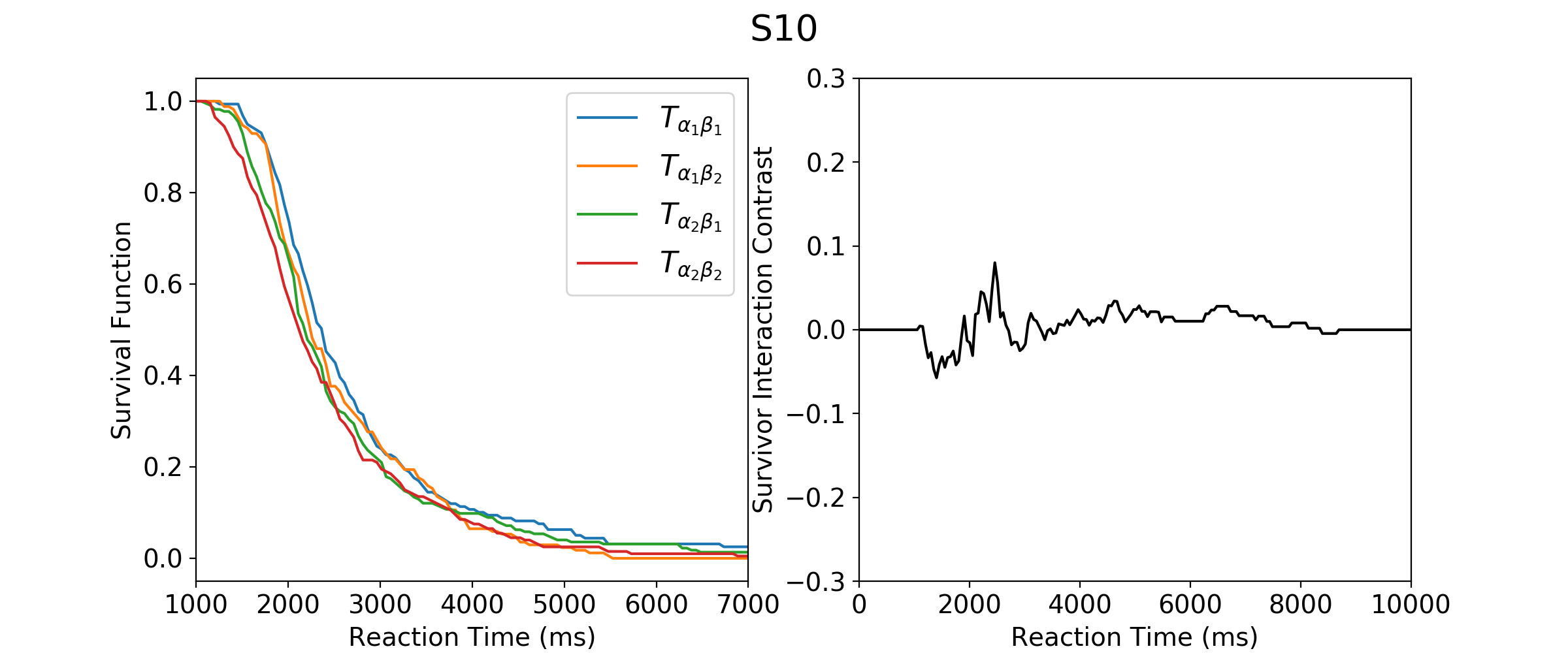
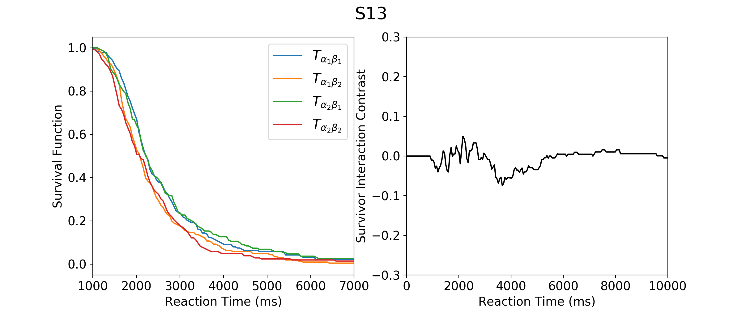
Figure 4: Survival functions of RT and SIC for S1, S7, S10, S13, and S14 in Experiment 1. S1 participated in Experiment 1(a). S7 and S10 participated in Experiment 1(b). S13 and S14 participated in Experiment 1(c).

Figure 4: Survival functions of RT and SIC for S1, S7, S10, S13, and S14 in Experiment 1 (continued). S1 participated in Experiment 1(a). S7 and S10 participated in Experiment 1(b). S13 and S14 participated in Experiment 1(c).

S1 and S7 agreed with the characteristic properties for parallel AND as $D^{-}$ was significant, $D^{+}$ was not significant, and MIC was significantly smaller than zero. $D^{+}$, $D^{-}$, and MIC for S10 and S13 were not significantly different from zero, indicating a lack of statistical power to draw a conclusion. For S14, he/she had a significant $D^{-}$ and insignificant $D^{+}$, which favored the parallel AND model. However this subject did not have a significant MIC, which was not aligned with parallel AND. To be cautious, we conclude that S14’s strategy was uncertain. In the very beginning we expected that all the subjects in this experiment adjusted the coordinates of the test dots in the parallel AND or serial AND or coactive manner. The trajectory of the trackball movements excluded serial AND. The architectures inferred for S1, S7, S10, S13, and S14 were either parallel AND or uncertain, which was consistent with the earlier expectation and the trackball move.

Table 11: The statistics of SIC and MIC and the inferred architectures for S1, S7, S10, S13, and S14 in Experiment 1. S1 participated in Experiment 1(a). S7 and S10 participated in Experiment 1(b). S13 and S14 participated in Experiment 1(c).

Subject	$D^{+}$($p$ value)	$D^{-}$($p$ value)	MIC($p$ value)	Architecture
S1	.038(.733)	.105(.096)	-271.47(.144)	Parallel AND
S7	.030(.921)	.269(.001)	-145.48(.014)	Parallel AND
S10	.085(.522)	.083(.538)	54.74(.895)	-
S13	.085(.510)	.076(.582)	-65.234(.999)	-
S14	.050(.795)	.111(.321)	103.86(.592)	Uncertain

Estimating Capacity

As mentioned in the beginning of this article, DFP includes two types of manipulation. In Experiments 1(b) and 1(c), we manipulated the workload by adding some reference dots with either the horizontal coordinate or the vertical coordinate equal to 0 px. So sometimes one channel was loaded to the subjects’ action as they had to adjust only one coordinate of the test dot and in the other trials two channels were loaded. The manipulation of stimulus salience was realized by assigning the horizontal coordinate of the reference dot to level one ($\alpha_{1}$) or level two ($\alpha_{2}$) and the vertical coordinate to level one ($\beta_{1}$) or level two ($\beta_{2}$), so the processing speed of level 1 was slower than the speed of level 2. In the DFP, there are eight types of stimuli. The trials display stimuli $\alpha_{0}\beta_{1}$, $\alpha_{0}\beta_{2}$, $\alpha_{1}\beta_{0}$, and $\alpha_{2}\beta_{0}$ are single-channel trials. The trials display stimuli $\alpha_{1}\beta_{1}$, $\alpha_{1}\beta_{2}$, $\alpha_{2}\beta_{1}$, and $\alpha_{2}\beta_{2}$ are double-channel trials. In Experiment 1(b), the double-channel trials and the single-channel trials were presented to the subjects in an intermixed way: In each trial, each of the eight stimuli had the same chance to be shown. In Experiment 1(b), the double-channel trials and the single-channel trials were presented in the separate experimental sessions.

We anticipated the subjects in Experiment 1 used the AND stopping rule to make responses as both the horizontal coordinate and the vertical coordinate of the test dot had to match those of the reference dot. The experimental design of Experiment 1(b) and 1(c) allowed the computation of $K_{\alpha\beta}(t)$, $K_{\beta}(t)$, and $K_{\alpha}(t)$ in (6): $K_{\alpha\beta}(t)$ was computed from the double-channel trials, $K_{\beta}(t)$ was from the single-channel trials with stimuli $\alpha_{0}\beta_{1}$ and $\alpha_{0}\beta_{2}$, and $K_{\alpha}(t)$ was from the stimuli $\alpha_{1}\beta_{0}$ and $\alpha_{2}\beta_{0}$.

The statistics of the capacity coefficient was computed using the R package developed by Houpt, Blaha, McIntire, Havig, and Townsend (2014). The capacity for S7, S10, and S13 (Figure 5) was super ($p<.001$) indicating adding one channel speeded up the processing of the other channel and for S14 it was limited indicating adding one channel slowed down the other channel.

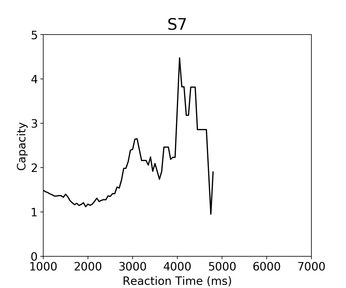
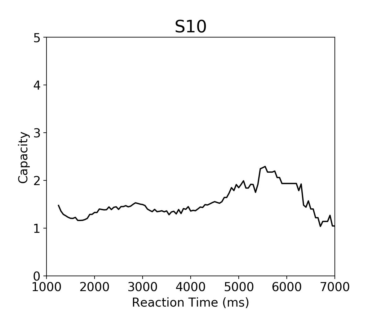
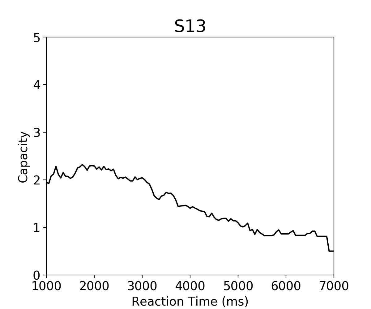
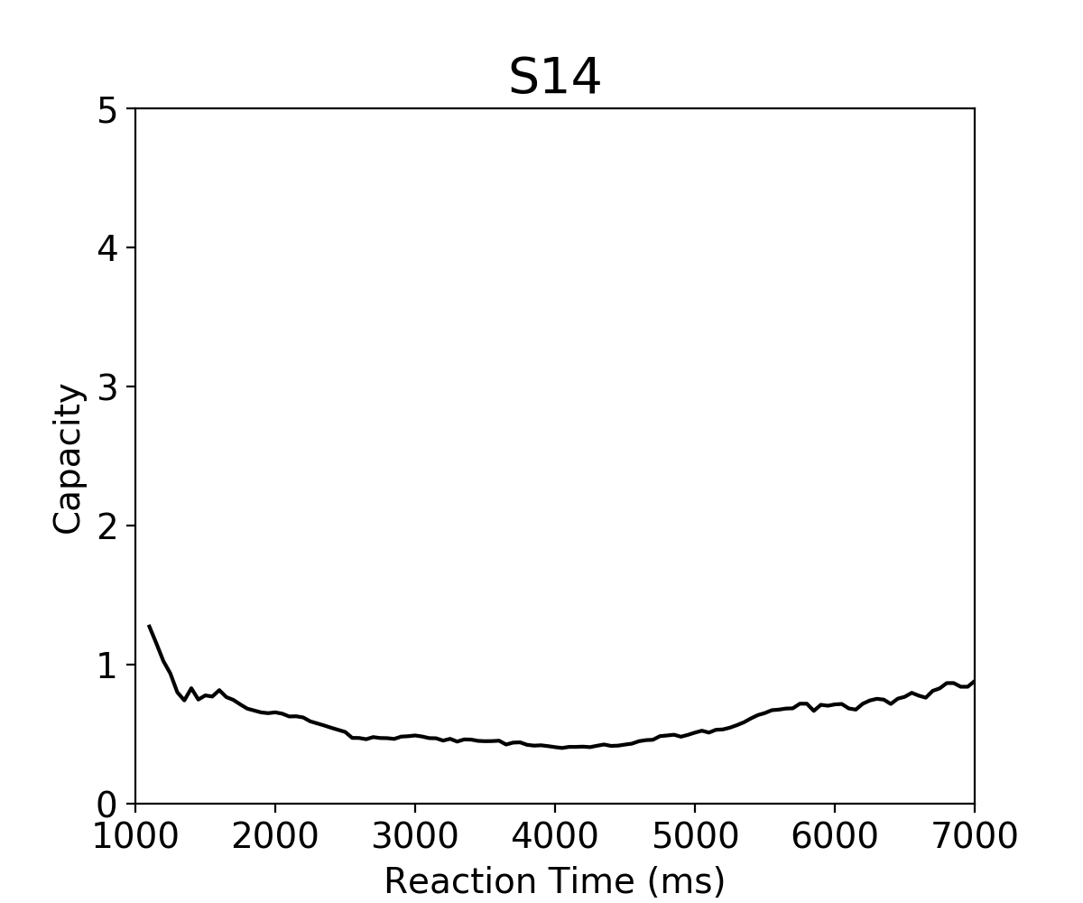
Figure 5: The capacity coefficients for S7, S10, S13, and S14 in Experiment 1. S7 and S10 participated in Experiment 1(b). S13 and S14 participated in Experiment 1(c).

The Consequence of Absence of $(A,B)\looparrowleft(\alpha,\beta)$

Subject S2, S3, S8, S9, S11, S12, S15, and S16 did not pass the test for $(A,B)\looparrowleft(\alpha,\beta)$. We considered it a failure for the establishment of $(T_{\alpha},T_{\beta})\looparrowleft(\alpha,\beta)$. Those subjects all passed the test of stochastic dominance (Table 10). We investigated their architectures without the security of selective influence.

The right column of Figure 6 displays the SIC curves for S2, S3, S8, S9, S11, S12, S15, and S16. The statistics for SIC and MIC and the inferred architectures for these subjects can be found in Table 12. $D^{+}$ was significant and $D^{-}$ was not significant ($\mathrm{alpha}=.33$) for S2, favoring the parallel OR model. However MIC for this subject was not significantly greater than zero, which was not consistent with the property for parallel OR. Therefore we considered the architecture for this subject uncertain as the conclusions from SIC and MIC did not converge. The referred architecture indicates S3 implemented the parallel OR manner to make responses as $D^{+}$ was significant, $D^{-}$ was not significant, and MIC was significantly greater than zero. Subject S8, S11, S12, and S16’s SIC and MIC were not significant, then we considered their architectures were not diagnostic. For subject S9, $D^{+}$ was not significant, $D^{-}$ was significant, and MIC was significantly smaller than zero, supporting the parallel AND signature. For S15, $D^{+}$ was not significant and $D^{-}$ was significant, favoring the parallel AND model. However MIC was not significantly different than zero, which did not align with parallel AND. Therefore we considered the architecture for this person uncertain. For the subjects examined in this section, we observed a prohibited signature: parallel OR for S3. The diagnosis for S3 seemed questionable.

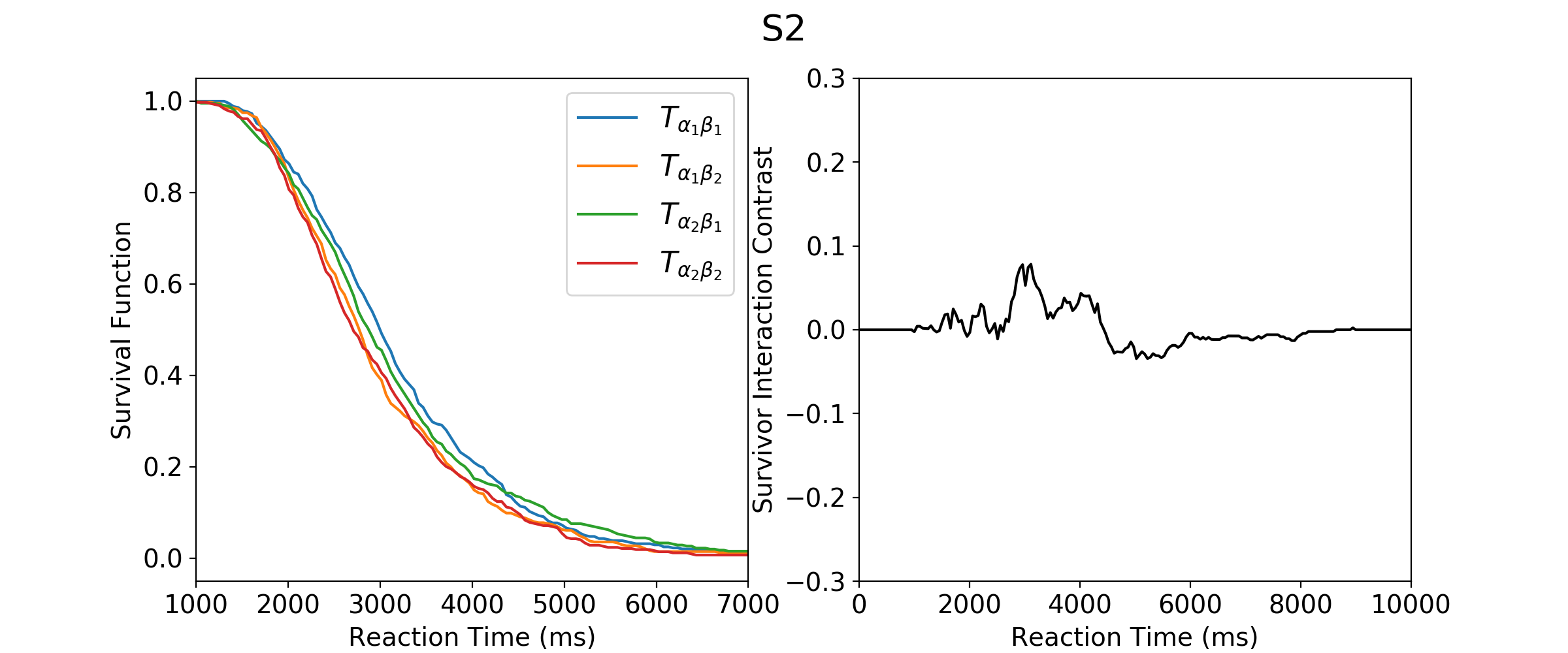
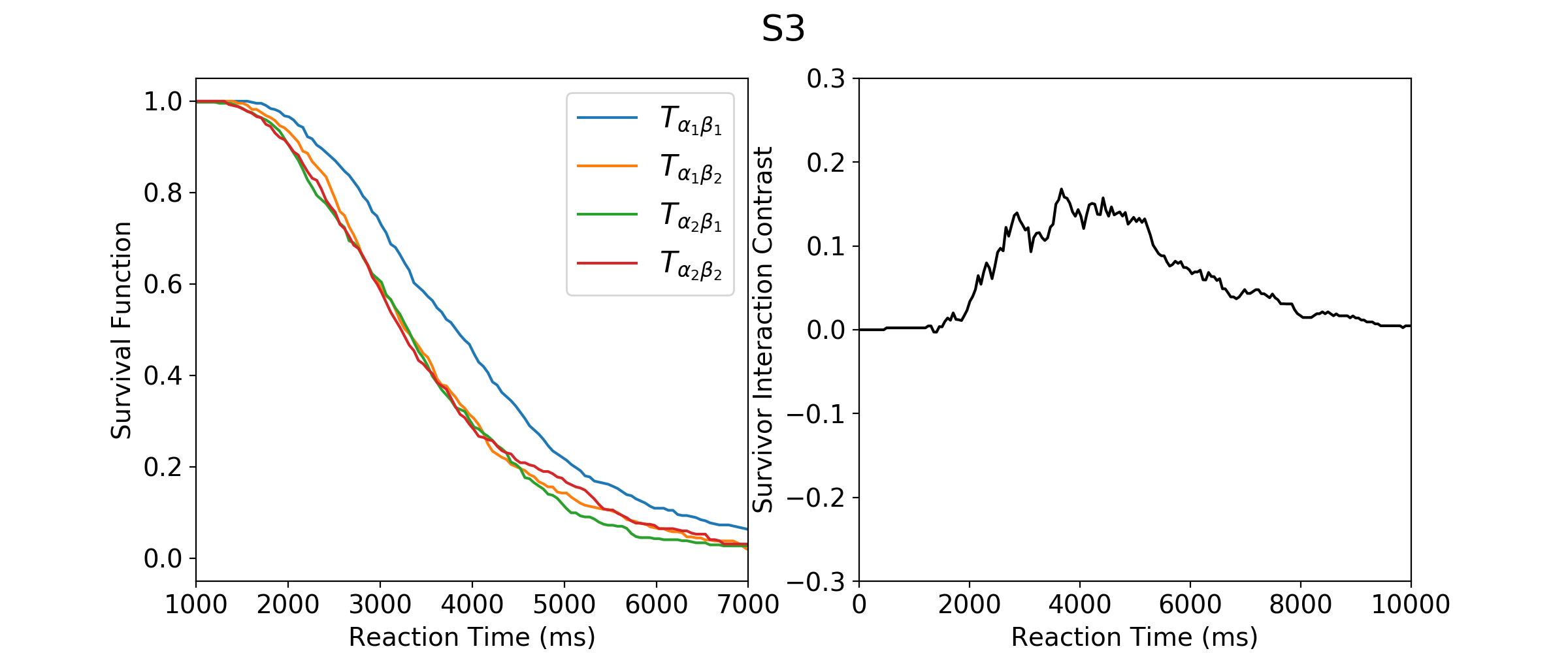
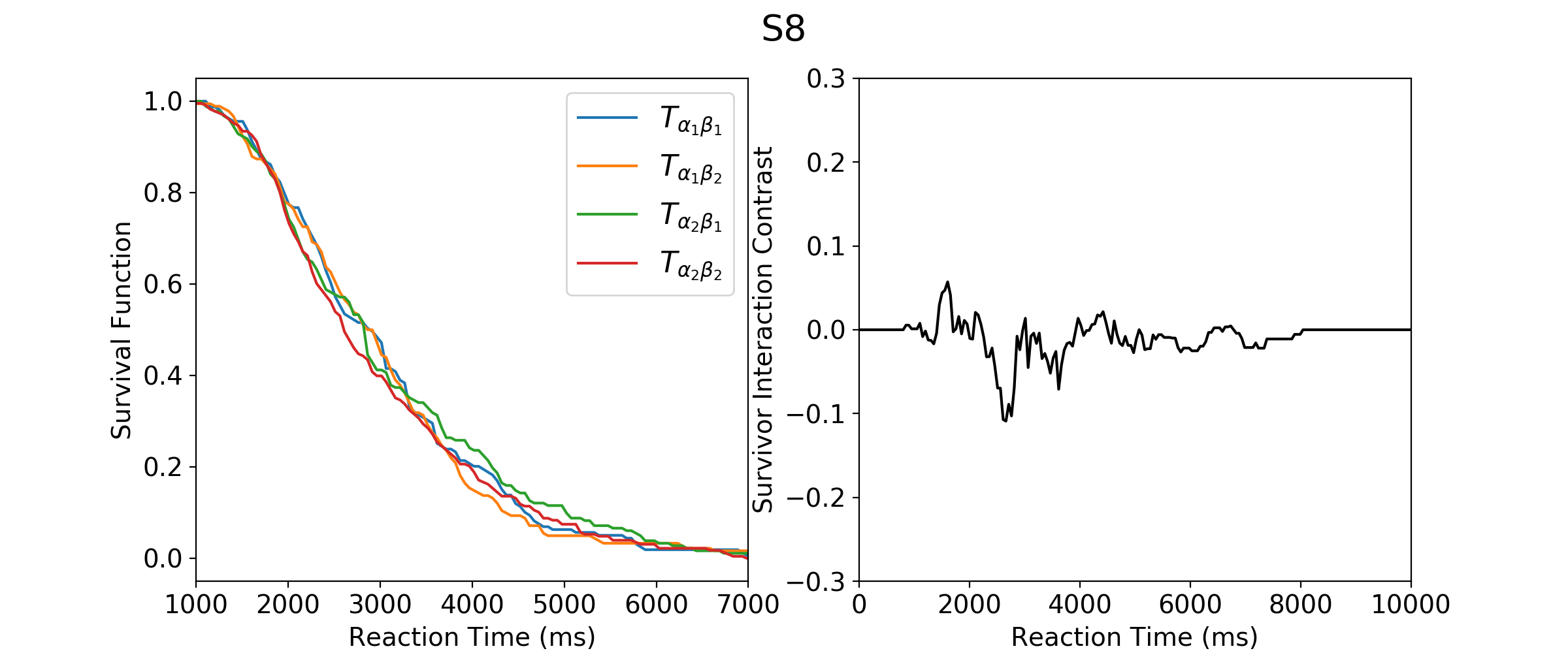
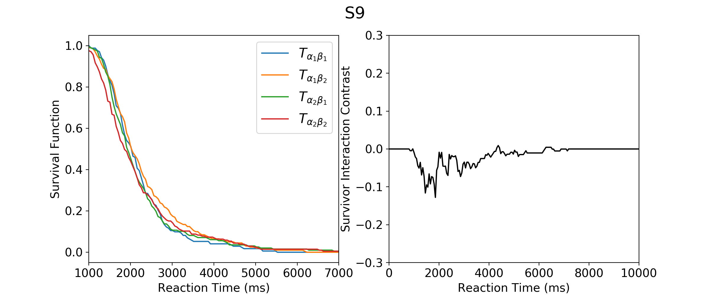
Figure 6: Survival functions of RT and SIC for S2, S3, S8, S9, S11, S12, S15, and S16 in Experiment 1. S2 and S3 participated in Experiment 1(a). S8, S9, and S11 participated in Experiment 1(b). S12, S15, and S16 participated in Experiment 1(c).

Figure 6: Survival functions of RT and SIC for S2, S3, S8, S9, S11, S12, S15, and S16 in Experiment 1 (continued). S2 and S3 participated in Experiment 1(a). S8, S9, and S11 participated in Experiment 1(b). S12, S15, and S16 participated in Experiment 1(c).

Table 12: The statistics of SIC and MIC and the inferred architectures for S2, S3, S8, S9, S11, S12, S15, and S16 in Experiment 1. S2 and S3 participated in Experiment 1(a). S8, S9, and S11 participated in Experiment 1(b). S12, S15, and S16 participated in Experiment 1(c).

Subject	$D^{+}$($p$ value)	$D^{-}$($p$ value)	MIC($p$ value)	Architecture
S2	.085(.210)	.036(.761)	8.65(.544)	Uncertain
S3	.159(.005)	.005(.995)	563.25(.000)	Parallel OR
S8	.069(.649)	.088(.495)	-23.637(.951)	-
S9	.009(.993)	.138(.173)	-169.08(.199)	Parallel AND
S11	.074(.594)	.015(.980)	122.69(.485)	-
S12	.067(.656)	.068(.646)	-81.801(.835)	-
S15	.077(.574)	.133(.188)	67.986(.560)	Uncertain
S16	.059(.719)	.079(.553)	-39.131(.825)	-

Discussions

In this experiment, regardless of the test for $(A,B)\looparrowleft(\alpha,\beta)$ passed or not, stochastic dominance was not violated. However, given $(A,B)\looparrowleft(\alpha,\beta)$ established, the architectures diagnosed from SFT were not out of expectation. If $(A,B)\looparrowleft(\alpha,\beta)$ was absent, SFT led to an architecture that was indeed prohibited for one subject out of eight, which indicated an absence of $(T_{\alpha},T_{\beta})\looparrowleft(\alpha,\beta)$ at least for that particular person. Therefore using stochastic dominance only as an evidence for selective influence of $\alpha$ and $\beta$ on $T_{\alpha}$ and $T_{\beta}$ is risky as it may result in an incorrect diagnosis about the architecture. Combining stochastic dominance and $(A,B)\looparrowleft(\alpha,\beta)$ results in a more trustable inference.

No single-channel trials were used in Experiment 1(a). In this experiment, we found that it took more time to move a test dot to the target location when the target was closer to the center of the circle. In Experiment 1(b), the participants had 50% chance to view a double-channel stimulus and 50% chance to view a single-channel stimulus in any trial. We found all the subjects spent more time to make a response when the reference dot was further to the center of the circle. In Experiment 1(c), the single-channel stimuli and the double-channel stimuli did not display to the participants in the mixed way. Rather the single-channel trials were presented only when all the double-channel trials were shown. We observed in Experiment 1(c) the RT was ordered in the same way as in Experiment 1(a) for four participants out of five. It indicates by mixing the single-channel trials with the double-channel trials in the experimental design, the ordering of RT for those double-channel trials was reversed. We name it context effect.

Floral Shape Reproduction Task

Trackball Movements

Figure 7 shows the trackball movements in a typical trial in the floral shape reproduction task. The trajectory of the trackball movements confirmed the assumption of SFT that the subject adheres to a single type of mental architecture from trial to trial. The red dot represents the amplitudes of the fixed reference shape. The test shape (blue) started from amplitudes (-31.828 px, -4.468 px) and after a sequence of adjustments for amplitude one and amplitude two, the finalized shape was very close to the target shape indicating the amplitudes were not adjusted in the parallel OR or serial OR or serial AND manner: If the stopping rule OR was used, one should expect the finalized test shape matched well with the reference shape either in amplitude one or amplitude two but not both. If serial AND was used, one should expect the trajectory moved only along the direction of amplitude one or along the direction of amplitude two in each step but not diagonally as observed in the plot. The trajectory implies parallel AND or coactive were used by the subjects in the task. However the trajectory is not able to differentiate parallel AND from coactive.

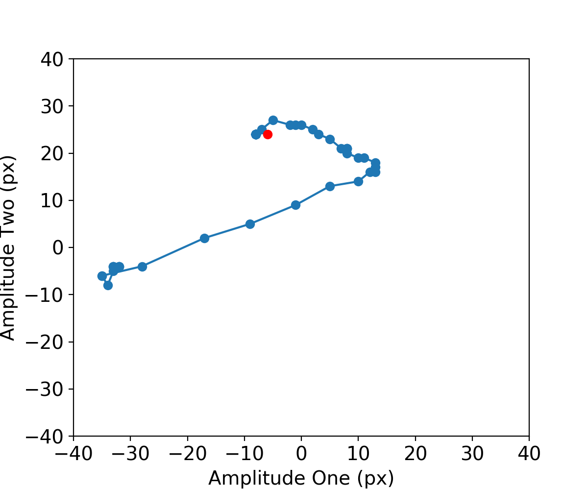
Figure 7: Typical trackball movements in a trial in the floral shape reproduction task (plotted every 50 ms).

Testing Selective Influence

In the dot position reproduction task, the dot move on the screen was directly reflected by the trackball move in the hand: If one moved the trackball to the right, the test dot also moved to the right. In the shape reproduction task, there was no apparent correspondence between the trackball move and the change of the shape: Each trackball move was transformed to the change of the amplitudes, defined by function (9). The horizontal and vertical coordinates of each shape was defined by the transformation from amplitudes (8). The transformation functions were designed for reasons. With these functions the floral shape reproduction task was not as straightforward as the dot position reproduction task to the participants, increasing the chance to have $A$ and $B$ selectively influenced by $\alpha$ and $\beta$. In addition as we can see from function (9), when $A$ or $B$ is negative, it is updated more sensitively to the move of the trackball than positive $A$ or $B$. So it was expected that RT was short when the reference shape had negative amplitudes and long with positive amplitudes.

In order to test selective influence of $\alpha$ and $\beta$ on the finalized $A$ and $B$, $\alpha$ and $\beta$ had to be discretized for instance:

$$\alpha_{1} =(0\,\mathrm{px},30\,\mathrm{px}],\alpha_{2}=[-30\,\mathrm{px},0\,\mathrm{px}],$$ (10)

$$\beta_{1} =(0\,\mathrm{px},30\,\mathrm{px}],\beta_{2}=[-30\,\mathrm{px},0\,\mathrm{px}].$$

The outliers of $A$ and $B$ were handled in this way: We computed $A-\alpha$ and $B-\beta$ for each trial. Any trial that was out of 3 standard deviations of the set of $A-\alpha$ or $B-\beta$ was considered as an outlier and was removed from further analysis. Table 13 presents the corresponding means and standard deviations of $A$ and $B$ for Experiment 2.

Table 13: Means and standard deviations of the finalized amplitudes of the test shapes for Experiment 2.

Exp.	Subject	$((0\,\mathrm{px},30\,\mathrm{px}],(0\,\mathrm{px},30\,\mathrm{px}])$, $((0\,\mathrm{px},30\,\mathrm{px}],[-30\,\mathrm{px},0\,\mathrm{px}])$, $([-30\,\mathrm{px},0\,\mathrm{px}],(0\,\mathrm{px},30\,\mathrm{px}])$, $([-30\,\mathrm{px},0\,\mathrm{px}],[-30\,\mathrm{px},0\,\mathrm{px}])$
2(a)	S4	$(15.69\pm 8.93,15.86\pm 8.93)$, $(14.39\pm 8.98,-15.74\pm 9.23)$, $(-14.66\pm 8.97,15.05\pm 9.53)$, $(-14.73\pm 9.47,-15.25\pm 9.02)$
2(a)	S5	$(14.91\pm 8.05,15.48\pm 8.71)$, $(14.43\pm 8.41,-14.97\pm 8.58)$, $(-14.33\pm 8.78,15.21\pm 8.44)$, $(-14.55\pm 8.52,-15.03\pm 8.09)$
2(a)	S6	$(14.36\pm 9.34,13.74\pm 8.70)$, $(14.67\pm 9.00,-15.26\pm 8.48)$, $(-14.95\pm 9.25,14.14\pm 8.26)$, $(-15.94\pm 8.77,-15.52\pm 8.71)$
2(b)	S1	$(15.95\pm 8.63,15.00\pm 8.21)$, $(15.25\pm 8.46,-14.62\pm 8.51)$, $(-14.65\pm 8.21,14.83\pm 8.34)$, $(-13.60\pm 8.68,-15.05\pm 8.67)$
2(b)	S2	$(15.84\pm 8.75,14.50\pm 8.65)$, $(14.40\pm 9.17,-15.71\pm 8.73)$, $(-15.77\pm 8.54,14.99\pm 8.94)$, $(-14.33\pm 9.07,-15.23\pm 8.90)$
2(b)	S3	$(13.81\pm 8.78,14.95\pm 8.29)$, $(13.38\pm 9.12,-14.85\pm 9.41)$, $(-13.65\pm 8.62,14.60\pm 8.81)$, $(-15.46\pm 8.57,-15.40\pm 8.41)$
2(c)	S17	$(14.05\pm 12.64,13.20\pm 9.57)$, $(9.56\pm 12.34,-13.08\pm 10.76)$, $(-7.22\pm 12.94,14.61\pm 9.62)$, $(-13.64\pm 11.83,-14.60\pm 9.38)$
2(c)	S18	$(15.22\pm 8.73,14.79\pm 8.68)$, $(12.92\pm 9.35,-15.20\pm 9.01)$, $(-13.75\pm 8.36,14.57\pm 8.15)$, $(-15.04\pm 9.05,-16.12\pm 8.14)$
2(c)	S19	$(15.65\pm 8.79,14.93\pm 8.58)$, $(14.28\pm 8.82,-14.34\pm 7.67)$, $(-15.03\pm 8.50,13.74\pm 8.30)$, $(-14.21\pm 8.36,-14.06\pm 8.28)$
2(c)	S20	$(15.82\pm 9.00,15.18\pm 7.93)$, $(14.22\pm 9.22,-15.54\pm 8.38)$, $(-14.67\pm 8.77,14.65\pm 8.57)$, $(-17.91\pm 9.89,-15.26\pm 8.82)$
2(c)	S21	$(13.88\pm 9.72,15.10\pm 7.90)$, $(11.04\pm 10.16,-15.23\pm 9.15)$, $(-12.40\pm 10.11,15.82\pm 9.43)$, $(-16.88\pm 9.53,-14.42\pm 8.91)$

We then conducted four two sample KS tests for each subject to examine marginal selectivity (4): $T_{\alpha_{i}}$ and $T_{\beta_{j}}$ were replaced with $A_{i}$ and $B_{j}$ that stand for the amplitudes of the test shape conditional on the reference shape $\alpha_{i}\beta_{j},i,j\in\left\{1,2\right\}$. Table 14 presents the statistics for the tests. Each column of numbers represents a particular paired comparison for the subjects. For instance, $((0\,\mathrm{px},30\,\mathrm{px}],)$ compared the $A\mathrm{s}$ across different levels of $\beta$ but fixed $\alpha=(0\,\mathrm{px},30\,\mathrm{px}]$. $(,[-30\,\mathrm{px},0\,\mathrm{px}])$ compared the $B\mathrm{s}$ across different levels of $\alpha$ but fixed $\beta=[-30\,\mathrm{px},0\,\mathrm{px}]$. We conclude that marginal selectivity was confirmed for S4, S5, S6, S1, S18, and S19 ($\mathrm{alpha}=.05/4$).

Table 14: Two sample KS tests for marginal selectivity for Experiment 2.

Exp.	Subject	$((0\,\mathrm{px},30\,\mathrm{px}],)$	$([-30\,\mathrm{px},0\,\mathrm{px}],)$	$(,(0\,\mathrm{px},30\,\mathrm{px}])$	$(,[-30\,\mathrm{px},0\,\mathrm{px}])$	Marginal
						selectivity?
2(a)	S4	.069(.230)	.049(.653)	.084(.079)	.073(.186)	Yes
2(a)	S5	.049(.635)	.034(.952)	.054(.504)	.041(.855)	Yes
2(a)	S6	.062(.348)	.084(.089)	.070(.236)	.039(.876)	Yes
2(b)	S1	.057(.442)	.073(.191)	.037(.927)	.059(.388)	Yes
2(b)	S2	.094(.032)	.107(.008)	.054(.522)	.0620(.351)	No
2(b)	S3	.057(.476)	.120(.003)	.063(.336)	.078(.142)	No
2(c)	S17	.167(.009)	.211(.000)	.141(.034)	.089(.437)	No
2(c)	S18	.134(.046)	.148(.028)	.067(.742)	.120(.112)	Yes
2(c)	S19	.091(.394)	.070(.677)	.108(.174)	.081(.548)	Yes
2(c)	S20	.128(.070)	.199(.001)	.072(.701)	.115(.116)	No
2(c)	S21	.128(.094)	.197(.001)	.151(.018)	.082(.530)	No

Note: Each number outside of the brackets is the KS statistic value and each number in the brackets is the $p$ value.

For those who passed the test of marginal selectivity, we investigated if $(A,B)\looparrowleft(\alpha,\beta)$ secured by conducting LFT. We created two levels for $A$: {smaller than or equal to 0 px, larger than 0 px}, labeled as $\left\{a_{1},a_{2}\right\}$, and two levels for $B$: {smaller than or equal to 0 px, larger than 0 px}, labeled as $\left\{b_{1},b_{2}\right\}$. The numbers in the cells of Table 15 are the joint probabilities for the discretized $(A_{ij},\>B_{ij}),i,j\in\left\{1,2\right\}$, and the numbers outside are the marginal probabilities.

Table 15: Joint distributions of the discretized $(A_{ij},\>B_{ij}),i,j\in\left\{1,2\right\}$ for S4, S5, S6, S1, S18, and S19 in Experiment 2. S4, S5, and S6 participated in Experiment 2(a). S1 participated in Experiment 2(b). S18 and S19 participated in Experiment 2(c).

S4
$\alpha_{1}\beta_{1}$	$B_{11}=b_{1}$	$B_{11}=b_{2}$		$\alpha_{1}\beta_{2}$	$B_{12}=b_{1}$	$B_{12}=b_{2}$
$A_{11}=a_{1}$	0	.0271	.0271	$A_{12}=a_{1}$	.0505	0	.0505
$A_{11}=a_{2}$	.0146	.9583	.9729	$A_{12}=a_{2}$	.9183	.0313	.9496
	.0146	.9854			.9688	.0313
$\alpha_{2}\beta_{1}$	$B_{21}=b_{1}$	$B_{21}=b_{2}$		$\alpha_{2}\beta_{2}$	$B_{22}=b_{1}$	$B_{22}=b_{2}$
$A_{21}=a_{1}$	.0370	.9261	.9631	$A_{22}=a_{1}$	.9214	.0175	.9389
$A_{21}=a_{2}$	0	.0370	.0370	$A_{22}=a_{2}$	.0611	0	.0611
	.0370	.9631			.9825	.0175

S5
$\alpha_{1}\beta_{1}$	$B_{11}=b_{1}$	$B_{11}=b_{2}$		$\alpha_{1}\beta_{2}$	$B_{12}=b_{1}$	$B_{12}=b_{2}$
$A_{11}=a_{1}$	0	.0134	.0134	$A_{12}=a_{1}$	.0312	0	.0312
$A_{11}=a_{2}$	.0201	.9664	.9865	$A_{12}=a_{2}$	.9310	.0379	.9689
	.0201	.9798			.9622	.0379
$\alpha_{2}\beta_{1}$	$B_{21}=b_{1}$	$B_{21}=b_{2}$		$\alpha_{2}\beta_{2}$	$B_{22}=b_{1}$	$B_{22}=b_{2}$
$A_{21}=a_{1}$	.0299	.9124	.9423	$A_{22}=a_{1}$	.9531	.0094	.9625
$A_{21}=a_{2}$	0	.0577	.0577	$A_{22}=a_{2}$	.0376	0	.0376
	.0299	.9701			.9907	.0094

S6
$\alpha_{1}\beta_{1}$	$B_{11}=b_{1}$	$B_{11}=b_{2}$		$\alpha_{1}\beta_{2}$	$B_{12}=b_{1}$	$B_{12}=b_{2}$
$A_{11}=a_{1}$	.0023	.0465	.0488	$A_{12}=a_{1}$	.0458	0	.0458
$A_{11}=a_{2}$	.0256	.9256	.9512	$A_{12}=a_{2}$	.9259	.0283	.9542
	.0279	.9721			.9717	.0283
$\alpha_{2}\beta_{1}$	$B_{21}=b_{1}$	$B_{21}=b_{2}$		$\alpha_{2}\beta_{2}$	$B_{22}=b_{1}$	$B_{22}=b_{2}$
$A_{21}=a_{1}$	.0393	.9076	.9469	$A_{22}=a_{1}$	.9438	.0202	.9640
$A_{21}=a_{2}$	0	.0531	.0531	$A_{22}=a_{2}$	.0360	0	.0360
	.0393	.9607			.9798	.0202

S1
$\alpha_{1}\beta_{1}$	$B_{11}=b_{1}$	$B_{11}=b_{2}$		$\alpha_{1}\beta_{2}$	$B_{12}=b_{1}$	$B_{12}=b_{2}$
$A_{11}=a_{1}$	0	.0343	.0343	$A_{12}=a_{1}$	.0277	0	.0277
$A_{11}=a_{2}$	.0114	.9542	.9656	$A_{12}=a_{2}$	.9574	.0149	.9723
	.0114	.9885			.9851	.0149
$\alpha_{2}\beta_{1}$	$B_{21}=b_{1}$	$B_{21}=b_{2}$		$\alpha_{2}\beta_{2}$	$B_{22}=b_{1}$	$B_{22}=b_{2}$
$A_{21}=a_{1}$	.0046	.9771	.9817	$A_{22}=a_{1}$	.9452	.0160	.9612
$A_{21}=a_{2}$	0	.0183	.0183	$A_{22}=a_{2}$	.0388	0	.0388
	.0046	.9954			.9840	.0160

Table 15: Joint distributions of the discretized $(A_{ij},\>B_{ij}),i,j\in\left\{1,2\right\}$ for S4, S5, S6, S1, S18, and S19 in Experiment 2 (continued). S4, S5, and S6 participated in Experiment 2(a). S1 participated in Experiment 2(b). S18 and S19 participated in Experiment 2(c).

S18
$\alpha_{1}\beta_{1}$	$B_{11}=b_{1}$	$B_{11}=b_{2}$		$\alpha_{1}\beta_{2}$	$B_{12}=b_{1}$	$B_{12}=b_{2}$
$A_{11}=a_{1}$	0	.0381	.0381	$A_{12}=a_{1}$	.0896	0	.0896
$A_{11}=a_{2}$	.0095	.9523	.9618	$A_{12}=a_{2}$	.8806	.0299	.9105
	.0095	.9904			.9702	.0299
$\alpha_{2}\beta_{1}$	$B_{21}=b_{1}$	$B_{21}=b_{2}$		$\alpha_{2}\beta_{2}$	$B_{22}=b_{1}$	$B_{22}=b_{2}$
$A_{21}=a_{1}$	.0105	.9634	.9739	$A_{22}=a_{1}$	.9521	.0106	.9627
$A_{21}=a_{2}$	0	.0262	.0262	$A_{22}=a_{2}$	.0372	0	.0372
	.0105	.9896			.9893	.0106

S19
$\alpha_{1}\beta_{1}$	$B_{11}=b_{1}$	$B_{11}=b_{2}$		$\alpha_{1}\beta_{2}$	$B_{12}=b_{1}$	$B_{12}=b_{2}$
$A_{11}=a_{1}$	0	.0204	.0204	$A_{12}=a_{1}$	.0718	0	.0718
$A_{11}=a_{2}$	.0102	.9694	.9796	$A_{12}=a_{2}$	.9116	.0166	.9282
	.0102	.9898			.9834	.0166
$\alpha_{2}\beta_{1}$	$B_{21}=b_{1}$	$B_{21}=b_{2}$		$\alpha_{2}\beta_{2}$	$B_{22}=b_{1}$	$B_{22}=b_{2}$
$A_{21}=a_{1}$	.0474	.8957	.9431	$A_{22}=a_{1}$	.9646	.0051	.9697
$A_{21}=a_{2}$	0	.0569	.0569	$A_{22}=a_{2}$	.0303	0	.0303
	.0474	.9526			.9949	.0051

The equations (4) did not strictly hold in Table 15. We modified the values of the marginal probabilities and joint probabilities for each subject in the same way as in Experiment 1. We were able to find nonnegative solutions for LFT (Table 16), indicating selective influence of $\alpha$ and $\beta$ on $A$ and $B$ was established for S4, S5, S6, S1, S18, and S19. Of course one can choose values other than 0 px to discretize $A$ or $B$. We found LFT passed for all the other values that we tried. We then considered $(T_{\alpha},T_{\beta})\looparrowleft(\alpha,\beta)$ was successfully established for these subjects.

Table 16: Solutions for LFT for S4, S5, S6, S1, S18, and S19 in Experiment 2. S4, S5, and S6 participated in Experiment 2(a). S1 participated in Experiment 2(b). S18 and S19 participated in Experiment 2(c).

Subject	$(Q_{a_{1}a_{1}b_{1}b_{1}},\,Q_{a_{1}a_{1}b_{1}b_{2}},\,\ldots,\,Q_{a_{2}a_{2}b_{2}b_{2}})^{T}$
S4	$(0,0,0,0,0,0,.0388,0,.0014,.0244,.9252,0,0,0,.0102,0)^{T}$
S5	$(0,0,0,0,0,0,.0223,0,.0014,.0236,.9274,0,0,0,.0253,0)^{T}$
S6	$(.0023,0,.0131,0,0,0,.0319,0,.0197,.0116,.9087,0,0,0,0,.0127)^{T}$
S1	$(0,0,.0026,.0033,0,0,.0251,0,0,.0046,.9535,.0075,.0034,0,0,0)^{T}$
S18	$(0,0,.0361,0,0,0,.0277,0,0,.01,.916,.0062,0,0,0,.004)^{T}$
S19	$(0,0,.0026,0,0,0,.0436,0,.018,.0108,.925,0,0,0,0,0)^{T}$

Testing Stochastic Dominance

We tested the assumption of stochastic dominance (5) for all the participants in Experiment 2. For each participant, we considered any trial with RT outside of 5 standard deviations of the set of RTs an outlier and it was not included in the further analysis.

The left column of Figure 8 presents the survival functions of RT for the subjects who passed the test for $(A,B)\looparrowleft(\alpha,\beta)$. Two one tail KS tests were performed on each of the four paired variables (5). The statistical results (Table 17) support the assumption of stochastic dominance for these subjects with the assignment (10) as for each subject the $p$ values in the bottom row were larger than the critical value $\mathrm{alpha}=.05/4$. Note for S1, the $p$ value for $S_{\alpha_{1}\beta_{1}}<S_{\alpha_{2}\beta_{1}}$ was not larger than the critical value. We loosely considered S1 passed the test of stochastic dominance as $p=.011$ was close to the critical value and other paired comparisons of this person passed the statistical criterion.

Subject S2, S3, S17, S20, and S21 did not pass the test of selective influence. We found that the ordering of RT was tortured for S2, S3, S17, and S21. For S3 and S17, the RT for the stimuli with opposite signs of amplitudes consumed more time to make responses than the stimuli with the same sign of amplitudes. For S2, the RT for stimulus $\alpha_{1}\beta_{2}$ was the shortest. For S20, we found $S_{\alpha_{2}\beta_{1}}>S_{\alpha_{1}\beta_{1}}>S_{\alpha_{2}\beta_{2}}>S_{\alpha_{1}\beta_{2}}$. S21 passed the test of stochastic dominance (Table 18) and the ordering of survival functions was plotted in the left column of Figure 9.

Table 17: One tail KS tests for stochastic dominance for S4, S5, S6, S1, S18, and S19 in Experiment 2. S4, S5, and S6 participated in Experiment 2(a). S1 participated in Experiment 2(b). S18 and S19 participated in Experiment 2(c).

S4
$S_{\alpha_{1}\beta_{1}}>S_{\alpha_{1}\beta_{2}}$	$S_{\alpha_{1}\beta_{1}}>S_{\alpha_{2}\beta_{1}}$	$S_{\alpha_{1}\beta_{2}}>S_{\alpha_{2}\beta_{2}}$	$S_{\alpha_{2}\beta_{1}}>S_{\alpha_{2}\beta_{2}}$
.035(.580)	.040(.489)	.141(.000)	.151(.000)
$S_{\alpha_{1}\beta_{1}}<S_{\alpha_{1}\beta_{2}}$	$S_{\alpha_{1}\beta_{1}}<S_{\alpha_{2}\beta_{1}}$	$S_{\alpha_{1}\beta_{2}}<S_{\alpha_{2}\beta_{2}}$	$S_{\alpha_{2}\beta_{1}}<S_{\alpha_{2}\beta_{2}}$
.053(.285)	.081(.050)	.000(1.0)	.002(.997)
S5
$S_{\alpha_{1}\beta_{1}}>S_{\alpha_{1}\beta_{2}}$	$S_{\alpha_{1}\beta_{1}}>S_{\alpha_{2}\beta_{1}}$	$S_{\alpha_{1}\beta_{2}}>S_{\alpha_{2}\beta_{2}}$	$S_{\alpha_{2}\beta_{1}}>S_{\alpha_{2}\beta_{2}}$
.109(.005)	.043(.432)	.093(.023)	.161(.000)
$S_{\alpha_{1}\beta_{1}}<S_{\alpha_{1}\beta_{2}}$	$S_{\alpha_{1}\beta_{1}}<S_{\alpha_{2}\beta_{1}}$	$S_{\alpha_{1}\beta_{2}}<S_{\alpha_{2}\beta_{2}}$	$S_{\alpha_{2}\beta_{1}}<S_{\alpha_{2}\beta_{2}}$
.009(.961)	.018(.858)	.005(.990)	.002(.996)
S6
$S_{\alpha_{1}\beta_{1}}>S_{\alpha_{1}\beta_{2}}$	$S_{\alpha_{1}\beta_{1}}>S_{\alpha_{2}\beta_{1}}$	$S_{\alpha_{1}\beta_{2}}>S_{\alpha_{2}\beta_{2}}$	$S_{\alpha_{2}\beta_{1}}>S_{\alpha_{2}\beta_{2}}$
.238(.000)	.081(.063)	.095(.017)	.306(.000)
$S_{\alpha_{1}\beta_{1}}<S_{\alpha_{1}\beta_{2}}$	$S_{\alpha_{1}\beta_{1}}<S_{\alpha_{2}\beta_{1}}$	$S_{\alpha_{1}\beta_{2}}<S_{\alpha_{2}\beta_{2}}$	$S_{\alpha_{2}\beta_{1}}<S_{\alpha_{2}\beta_{2}}$
.020(.833)	.065(.168)	.004(.991)	.007(.978)
S1
$S_{\alpha_{1}\beta_{1}}>S_{\alpha_{1}\beta_{2}}$	$S_{\alpha_{1}\beta_{1}}>S_{\alpha_{2}\beta_{1}}$	$S_{\alpha_{1}\beta_{2}}>S_{\alpha_{2}\beta_{2}}$	$S_{\alpha_{2}\beta_{1}}>S_{\alpha_{2}\beta_{2}}$
.053(.284)	.027(.721)	.144(.000)	.220(.000)
$S_{\alpha_{1}\beta_{1}}<S_{\alpha_{1}\beta_{2}}$	$S_{\alpha_{1}\beta_{1}}<S_{\alpha_{2}\beta_{1}}$	$S_{\alpha_{1}\beta_{2}}<S_{\alpha_{2}\beta_{2}}$	$S_{\alpha_{2}\beta_{1}}<S_{\alpha_{2}\beta_{2}}$
.043(.429)	.102(.011)	.006(.986)	.007(.980)
S18
$S_{\alpha_{1}\beta_{1}}>S_{\alpha_{1}\beta_{2}}$	$S_{\alpha_{1}\beta_{1}}>S_{\alpha_{2}\beta_{1}}$	$S_{\alpha_{1}\beta_{2}}>S_{\alpha_{2}\beta_{2}}$	$S_{\alpha_{2}\beta_{1}}>S_{\alpha_{2}\beta_{2}}$
.098(.142)	.084(.245)	.144(.019)	.169(.005)
$S_{\alpha_{1}\beta_{1}}<S_{\alpha_{1}\beta_{2}}$	$S_{\alpha_{1}\beta_{1}}<S_{\alpha_{2}\beta_{1}}$	$S_{\alpha_{1}\beta_{2}}<S_{\alpha_{2}\beta_{2}}$	$S_{\alpha_{2}\beta_{1}}<S_{\alpha_{2}\beta_{2}}$
-2.082(1.0)	.023(.898)	1.306(1.0)	.000(1.0)
S19
$S_{\alpha_{1}\beta_{1}}>S_{\alpha_{1}\beta_{2}}$	$S_{\alpha_{1}\beta_{1}}>S_{\alpha_{2}\beta_{1}}$	$S_{\alpha_{1}\beta_{2}}>S_{\alpha_{2}\beta_{2}}$	$S_{\alpha_{2}\beta_{1}}>S_{\alpha_{2}\beta_{2}}$
.155(.011)	.076(.312)	.111(.099)	.308(.000)
$S_{\alpha_{1}\beta_{1}}<S_{\alpha_{1}\beta_{2}}$	$S_{\alpha_{1}\beta_{1}}<S_{\alpha_{2}\beta_{1}}$	$S_{\alpha_{1}\beta_{2}}<S_{\alpha_{2}\beta_{2}}$	$S_{\alpha_{2}\beta_{1}}<S_{\alpha_{2}\beta_{2}}$
.017(.948)	.147(.013)	.041(.728)	.011(.977)

Note: Each number outside of the brackets is the KS statistic value and each number in the brackets is the $p$ value.

Table 18: One tail KS tests for stochastic dominance for S21 in Experiment 2(c).

S21
$S_{\alpha_{1}\beta_{1}}>S_{\alpha_{1}\beta_{2}}$	$S_{\alpha_{1}\beta_{1}}>S_{\alpha_{2}\beta_{1}}$	$S_{\alpha_{1}\beta_{2}}>S_{\alpha_{2}\beta_{2}}$	$S_{\alpha_{2}\beta_{1}}>S_{\alpha_{2}\beta_{2}}$
.085(.265)	.029(.842)	.102(.142)	.178(.001)
$S_{\alpha_{1}\beta_{1}}<S_{\alpha_{1}\beta_{2}}$	$S_{\alpha_{1}\beta_{1}}<S_{\alpha_{2}\beta_{1}}$	$S_{\alpha_{1}\beta_{2}}<S_{\alpha_{2}\beta_{2}}$	$S_{\alpha_{2}\beta_{1}}<S_{\alpha_{2}\beta_{2}}$
.023(.906)	.064(.445)	.089(.225)	.014(.958)

Note: Each number outside of the brackets is the KS statistic value and each number in the brackets is the $p$ value.

Diagnosing Architectures According to SIC and MIC in the Presence of $(A,B)\looparrowleft(\alpha,\beta)$ and Stochastic Dominance

With the confirmation of the three assumptions for S4, S5, S6, S1, S18, and S19, we then diagnosed how the amplitudes of the test shape were adjusted by these subjects by investigating the behavior of SIC and MIC. The SIC curves are displayed in the right column of Figure 8. Table 19 includes the statistics for SIC and MIC and the inferred architectures from SFT. S4, S5, S1, and S18 were diagnosed to implement the parallel AND manner to adjust $A$ and $B$ as $D^{+}$ was not significant, $D^{-}$ was significant, and MIC was significantly less than zero ($\mathrm{alpha}=.33$). S6 had significant $D^{+}$ and $D^{-}$, which agreed with the signature of serial AND or coactive. The MIC of this person was positive but not significant, which seemed to support the model of serial AND. Or one can suspect it a lack of statistical power for a coactive model. Hence we conclude the architecture for S6 uncertain. S19 was coactive since $D^{+}$ and $D^{-}$ was significant and MIC was significantly greater than zero. Overall according to SFT, the strategies the subjects implemented in the floral shape reproduction task were either parallel AND or coactive, which were not contradicted with the researchers’ expectation and the trajectory of the trackball move.

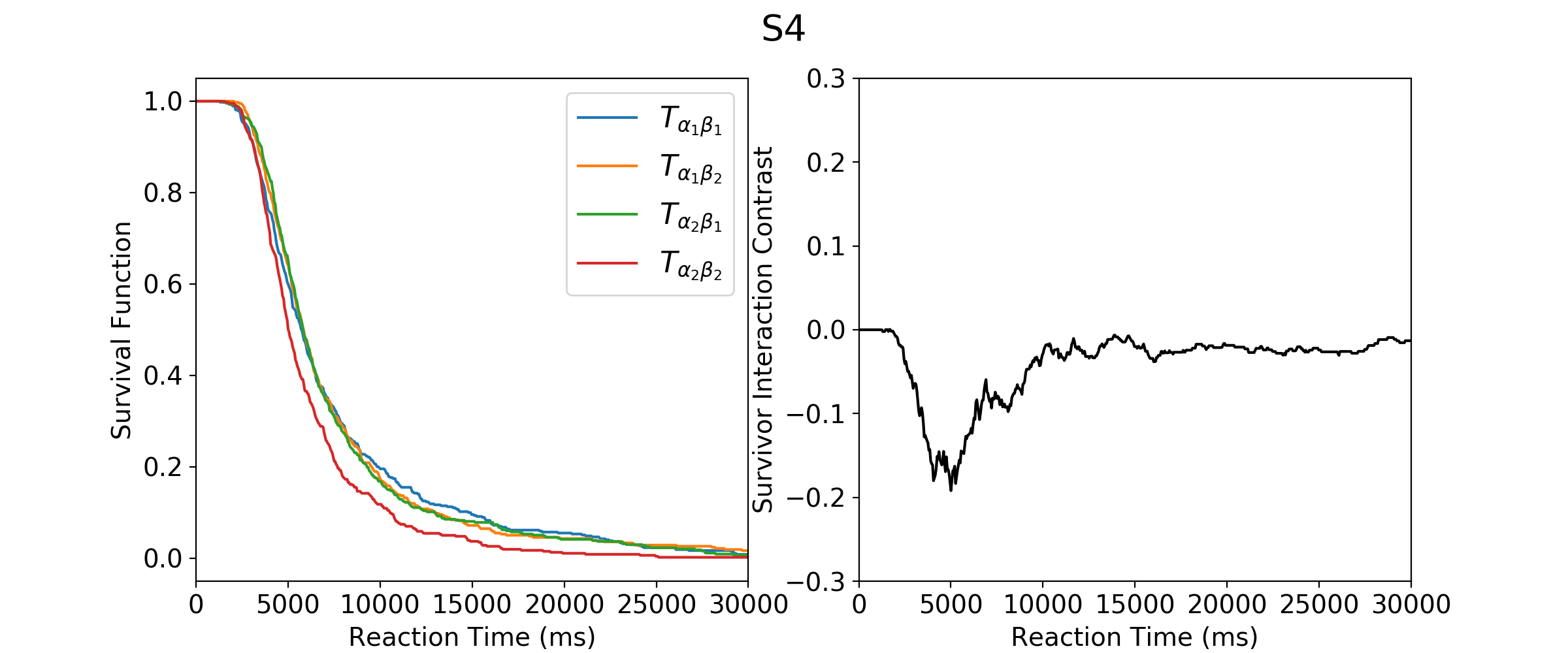
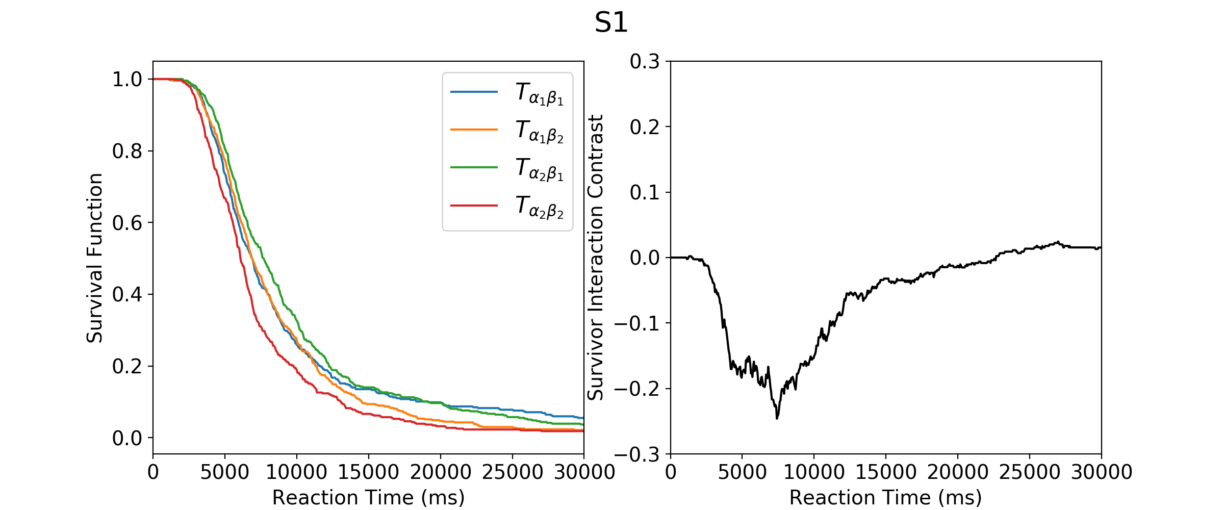
Figure 8: Survival functions of RT and SIC for S4, S5, S6, S1, S18, and S19 in Experiment 2. S4, S5, and S6 participated in Experiment 2(a). S1 participated in Experiment 2(b). S18 and S19 participated in Experiment 2(c).

Figure 8: Survival functions of RT and SIC for S4, S5, S6, S1, S18, and S19 in Experiment 2 (continued). S4, S5, and S6 participated in Experiment 2(a). S1 participated in Experiment 2(b). S18 and S19 participated in Experiment 2(c).

Table 19: The statistics of SIC and MIC and the inferred architectures for Experiment 2. S4, S5, and S6 participated in Experiment 2(a). S1 participated in Experiment 2(b). S18, S19, and S21 participated in Experiment 2(c).

Subject	$D^{+}$($p$ value)	$D^{-}$($p$ value)	MIC($p$ value)	Architecture
S4	.002(.999)	.191(.000)	-1189.2(.002)	Parallel AND
S5	.026(.864)	.095(.136)	-520.27(.234)	Parallel AND
S6	.080(.242)	.134(.019)	580.1(.436)	Uncertain
S1	.019(.921)	.253(.000)	-1636.6(.000)	Parallel AND
S18	.018(.968)	.155(.095)	-2178.9(.242)	Parallel AND
S19	.086(.487)	.208(.015)	202.41(.122)	Coactive
S21	.090(.457)	.147(.124)	-1163(.278)	Parallel AND

The Consequence of Absence of $(A,B)\looparrowleft(\alpha,\beta)$

Subject S2, S3, S17, S20, and S21 did not pass the test for $(A,B)\looparrowleft(\alpha,\beta)$. We considered it a failure for the establishment of $(T_{\alpha},T_{\beta})\looparrowleft(\alpha,\beta)$. S2, S3, S17, and S20 tortured the ordering of RT distributions, so it was impossible to investigate their SIC and MIC. Only S21 passed the test of stochastic dominance (Table 18). We investigated the architecture for this person even without the security of selective influence. The SIC curve of S21 is displayed in the right column of Figure 9. The statistics for SIC and MIC and the inferred architecture are in Table 19. The diagnosis was parallel AND because of nonsignificant $D^{+}$, significant $D^{-}$, and significant negative MIC ($\mathrm{alpha}=.33$).

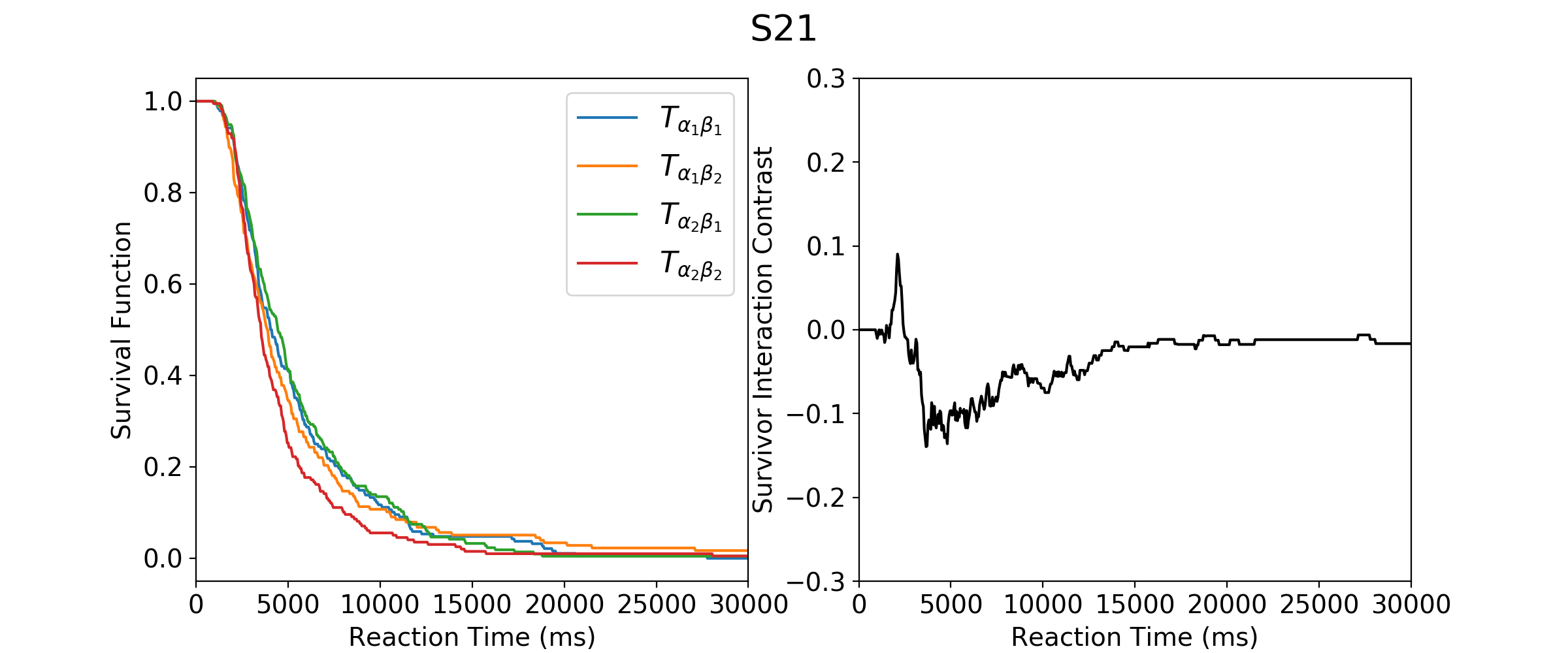
Figure 9: Survival functions of RT and SIC for S21 in Experiment 2(c).

Discussions

In this experiment, when the subjects passed the test for $(A,B)\looparrowleft(\alpha,\beta)$, the RTs were all ordered right and the diagnosed architectures were as anticipated: Some were parallel AND and some were coactive. By contrast if they failed the test for $(A,B)\looparrowleft(\alpha,\beta)$, four out of the five subjects’ ordering of RTs was tortured. The results in this experiment seem to imply a success of $(A,B)\looparrowleft(\alpha,\beta)$ was associated with a success of $(T_{\alpha},T_{\beta})\looparrowleft(\alpha,\beta)$; a failure of $(A,B)\looparrowleft(\alpha,\beta)$ was associated with a failure of $(T_{\alpha},T_{\beta})\looparrowleft(\alpha,\beta)$.

In Experiment 2, the chance to obtain $(A,B)\looparrowleft(\alpha,\beta)$ was 6 out of 11, higher than 5 out of 13 in Experiment 1, which met the earlier prediction. It indicates by removing the straightforward correspondence between hand move and the change of the test stimulus increases the chance of $(A,B)\looparrowleft(\alpha,\beta)$.

Experiment 2(c) replicated the results obtained from Experiment 2(b): There was no systematic difference between the two experiments in terms of the absence or presence of $(A,B)\looparrowleft(\alpha,\beta)$, the way the RTs were ordered, and the behavior of SIC and MIC.

Summary

We investigated how people moved the trackball in the trackball movement tasks through two lines of approach. One was the trajectory of the trackball movements and the other was SFT. According to the trajectory of trackball movements, we observed the subjects implemented parallel AND or coactive strategy (The trajectory cannot distinguish them) to adjust the location of the dot or modify the floral shape. SFT can distinguish the two strategies: In the shape reproduction task, some subjects implemented the parallel AND manner and some were coactive. The conclusions from the two lines of approach agreed with each other for both tasks.

We proposed a paradigm that can test the assumptions of SFT that are usually unobservable. In our paradigm, we recorded the physical parameters labeled as $A$ and $B$ in response to the stimulus features $\alpha$ and $\beta$ and the trajectory of $A$ and $B$ in addition to the reaction time for each trial. We showed that selective influence of $T_{\alpha}$ and $T_{\beta}$ can be established through testing selective influences of $A$ and $B$. The results indicate it is a valid approach since when $(A,B)\looparrowleft(\alpha,\beta)$ was established, the behavior of SIC and MIC was as anticipated; when the $(A,B)\looparrowleft(\alpha,\beta)$ was violated, the ordering of RT may break or the diagnosis about the architecture may be misleading.

Conventionally researchers consider stochastic dominance a successful establishment of selective influence for $T_{\alpha}$ and $T_{\beta}$. We agree stochastic dominance is correlated with selective influence $T_{\alpha}$ and $T_{\beta}$ to some extent, but stochastic dominance is neither a sufficient nor a necessary condition for $(T_{\alpha},T_{\beta})\looparrowleft(\alpha,\beta)$. Relying on stochastic dominance as an evidence of $(T_{\alpha},T_{\beta})\looparrowleft(\alpha,\beta)$ is risky as it can lead to an incorrect diagnosis for the architecture. However we understand due to the empirical limit, stochastic dominance can be the only way to exam $(T_{\alpha},T_{\beta})\looparrowleft(\alpha,\beta)$ as not all the experimental paradigms can afford recording $A$ and $B$ in response to $\alpha$ and $\beta$. Under this condition, we agree stochastic dominance is a useful test for $(T_{\alpha},T_{\beta})\looparrowleft(\alpha,\beta)$, but one should keep in mind these two properties are not equal to each other.

Another fundamental assumption for SFT is the subject uses only one architecture to make responses from trial to trial. This assumption is impossible to be tested in most studies. In our paradigm, we show, for the first time, the subjects indeed were stable with their strategies to respond to the stimuli as reflected by the trajectory over trials. It demonstrates at least in this particular paradigm, this assumption is valid.

One may suggest the exact values of $T_{\alpha}$ and $T_{\beta}$ can be estimated according to the moment the corresponding changing coordinates or amplitudes terminates. $(T_{\alpha},T_{\beta})\looparrowleft(\alpha,\beta)$ can then be tested using the values of $T_{\alpha}$ and $T_{\beta}$ rather than through testing $(A,B)\looparrowleft(\alpha,\beta)$. However this approach does not work as we frequently observed in a particular trial the subjects modified $A$ and $B$ simultaneously for a while then proceeded only $A$ or $B$ for a while and so on (e.g. Figure 7). It is practically impossible to estimate $T_{\alpha}$ and $T_{\beta}$ when they are broken in parts. So the values of $A$ and $B$ are a better map for the values of $T_{\alpha}$ and $T_{\beta}$.

We believe the experimental paradigm we have developed can be applied in other similar type of tasks, for instance eye-tracking. In the eye-tracking study, the physical parameters $A$ and $B$ in response to the stimulus features $\alpha$ and $\beta$ and the trajectory of $A$ and $B$ can be recorded in the similar way. Then one can inspect if $(T_{\alpha},T_{\beta})\looparrowleft(\alpha,\beta)$ holds by examining if $(A,B)\looparrowleft(\alpha,\beta)$ is present. With the establishment of $(T_{\alpha},T_{\beta})\looparrowleft(\alpha,\beta)$, SFT can be applied to diagnose the architecture and estimate capacity. SFT can provide deeper information about the architecture than observing the trajectory only: One cannot differentiate parallel AND from coactive according to the trajectory but SFT can tell the two models apart.

Moreover, most existing studies on mental architectures focus on the tasks with short response time. Subjects in those studies make a response within one second. In the current study, it usually took several seconds to make a response. Our work extends the application of SFT to a broader field.

The capacity coefficient can be estimated in Experiment 1. Experiment 2 did not allow the computation for capacity because of the absence of single-channel trials. In Experiment 2(a), 2(b), and 2(c), the amplitudes of the reference shapes were selected from the interval [-30 px, 30 px] and the amplitudes of the test shape were initialized randomly in the range [-35 px, 35 px]. In order to create the single-channel trials for this task, we introduced the reference shapes with amplitudes generated from [-30 px, 30 px] $\times$0 px or 0 px $\times$[-30 px, 30 px] and the test shapes were initialized with the amplitudes 0 px $\times$0 px. We observed the context effect regardless of if the single-channel trials and double-channel trials were displayed to the subjects in a mixed way or the single-channel trials came after all the double-channel trials were seen. The context effect we observed were the RT for the reference shapes with opposite-sign amplitudes were longer than those with same-sign amplitudes. Since the RTs were not ordered in an expected manner, the capacity was not computable.

Acknowledgements

This study was supported by NSF grant SES-1155956, AFOSR grant FA9550-14-1-0318, and MOST (Taiwan) grant 105-2410-H-006-020-MY2.

We thank Dr. Ehtibar Dzhafarov for the suggestions about the experimental design and the discussions about the concept of selective influence, ordering of RTs, and stochastic dominance.

References

- [1] Altieri, N., & Yang, C.-T. (2016). Parallel linear dynamic models can mimic the McGurk effect in clinical populations. Journal of Computational Neuroscience, 41(2), 143–155.
- [2] Dzhafarov, E.N., & Kujala, J.V. (2010). The Joint Distribution Criterion and the Distance Tests for selective probabilistic causality. Frontiers in Quantitative Psychology and Measurement, 1:151.
- [3] Eidels, A., Algom D., & Townsend, J.T. (2010). Comparing perception of Stroop stimuli in focused versus divided attention paradigms: Evidence for dramatic processing differences. Cognition, 114(2), 129-150.
- [4] Eidels, A., Pomerantz, J., & Townsend, J. T. (2008). Where Similarity Beats Redundancy: The Importance of Context, Higher Order Similarity, and Response Assignment. J Exp Psychol Hum Percept Perform, 34(6), 1441-1463.
- [5] Fifić, M., Little, D. R., & Nosofsky, R. (2010). Logical-rule models of classification response times: A synthesis of mental-architecture, random-walk, and decision-bound approaches. Psychological Review, 117, 309–48.
- [6] Fifić, M., & Townsend, J.T. (2010). Information-processing alternatives to holistic perception: Identifying the mechanisms of secondary-level holism within a categorization paradigm. Journal of Experimental Psychology: Learning, Memory, and Cognition. 36(5), 1290-1313.
- [7] Fifić, M., Townsend, J. T., & Eidels, A. (2008). Studying visual search using systems factorial methodology with target–distractor similarity as the factor. Percept Psychophys, 70(4), 583-603.
- [8] Fox, E., & Houpt, J.W. (2016). The perceptual processing of fused multispectral imagery. Cognitive research: Principles and implications.
- [9] Houpt, J.W., Blaha, L.M., McIntire, J.P., Havig, P.R., and Townsend, J.T. (2013). Systems factorial technology with R. Behavior Research Methods.
- [10] Johnson, S. A., Blaha, L.M., Houpt, J.W., & Townsend, J. T. (2010). Systems Factorial Technology provides new insights on global-local information processing in autism spectrum disorders. Journal of Mathematical Psychology, 54, 53-72.
- [11] Little, D. R., Altieri, N., Fific, M., & Yang, C.-T. (2017). Systems factorial technology: A theory driven methodology for the identification of perceptual and cognitive mechanisms. London, UK: Academic Press.
- [12] Schweickert, R., Giorgini, M., & Dzhafarov, E. N. (2000). Selective influence and response time cumulative distribution functions in serial-parallel task networks. Journal of Mathematical Psychology, 44, 504–535.
- [13] Sternberg, S. (1969) The discovery of processing stages: Extensions of Donders’ method. In W. G. Koster (Ed.), Attention and performance II. Acta Psychologica, 30, 276-315.
- [14] Townsend, J. T. & Fifić, M. (2004). Parallel & serial processing and individual differences in high-speed scanning in human memory. Perception & Psychophysics, 66, 953-962.
- [15] Townsend, J. T., & Nozawa, G. (1995). Spatio-temporal properties of elementary perception: An investigation of parallel, serial and coactive theories. Journal of Mathematical Psychology, 39, 321–360.
- [16] Townsend, J. T., & Schweickert, R. (1989). Toward the trichotomy method: Laying the foundation of stochastic mental networks. Journal of Mathematical Psychology, 33, 309-327.
- [17] Townsend, J. T. & Wenger, M.J. (2004). A theory of interactive parallel processing: New capacity measures and predictions for a response time inequality series. Psychological Review, 111, 1003-1035.
- [18] Wenger, M. J., & Townsend (2001). Faces as gestalt stimuli: Process characteristics. Chapter in book on face perception and cognition, edited by M. J. Wenger and J. T. Townsend. Erlbaum Press.
- [19] Yang, C.-T. (2011). Relative saliency in change signals affects perceptual comparison and decision processes in change detection. Journal of Experimental Psychology: Human Perception and Performance, 37(6), 1708-1728.
- [20] Yang, C.-T. (2017). Attention and perceptual decision making. In D. R. Little, N. Altieri, M. Fific, & C.-T. Yang (Eds). Systems factorial technology: A theory driven methodology for the identification of perceptual and cognitive mechanisms. (pp. 199-217). London, UK: Academic press.
- [21] Yang, C.-T., Altieri, N., & Little, D. R. (2018). An examination of parallel versus coactive processing accounts of redundant-target audiovisual signal processing. Journal of Mathematical Psychology, 82, 138-158.
- [22] Yang, C.-T., Fifić, M., Chang, T.-Y., & Little, D. R. (2018). Systems Factorial Technology provides new insights on the other-race effect. Psychonomic Bulletin & Review, 25(2), 596-604.
- [23] Yang, H., Fifić, M., & Townsend, J. T. (2013). Survivor interaction contrast wiggle predictions of parallel and serial models for an arbitrary number of processes. Journal of Mathematical Psychology, 58, 21–32.
- [24] Zhang, R. & Dzhafarov, E.N. (2015). Noncontextuality with marginal selectivity in reconstructing mental architectures. Frontier in Psychology, 6:735. doi: 10.3389/fpsyg.2015.00735