Fermi liquid approach for superconducting Kondo problems

Abstract

We present a Fermi liquid approach to superconducting Kondo problems applicable when the Kondo temperature is large compared to the superconducting gap. To illustrate the theory, we study the current-phase relation and the Andreev level spectrum for an Anderson impurity between two $s$-wave superconductors. In the particle-hole symmetric Kondo limit, we find a $4\pi$ periodic Andreev spectrum. The $4\pi$ periodicity persists under a small voltage bias which however causes an asymmetric distortion of Andreev levels. The latter distinguishes the present $4\pi$ effect from the one in topological Majorana junctions.

Introduction.—The interplay between superconductivity and localized magnetic moments remains of central importance to modern condensed-matter physics. For instance, spin-fluctuation mediated pairing is encountered in a broad variety of unconventional superconducting materials Hewson ; Scalapino2012 . Moreover, Yu-Shiba-Rusinov states induced by a magnetic impurity in a superconductor Yu1965 ; Shiba1968 ; Rusinov1969 can be responsible for Majorana bound states in magnetic atom chains deposited on superconducting substrates Yazdani2014 ; Franke2015 . A paradigmatic example for superconducting Kondo problems is given by an Anderson dot in the magnetic regime (where it can realize a Kondo impurity) sandwiched between two conventional $s$-wave BCS superconductors Glazman1989 ; Rozhkov1999 ; Avishai2003 ; Vecino2003 ; Yeyati2003 ; Siano2004 ; Choi2004 ; Sellier2005 ; Bergeret2006 ; Luca2008 ; Karrasch2008 ; Meng2009 ; Andersen2011 ; Alvaro2011 ; Luitz2012 ; Meden2014 , with experimental realizations available in nanoscale devices Kasumov1999 ; VanDam2006 ; Cleuziou2006 ; Jorgensen2007 ; Sand-Jespersen2007 ; Eichler2009 ; Delagrange2015 . Numerical calculations Siano2004 ; Choi2004 ; Karrasch2008 ; Luitz2012 show that the low-temperature physics is governed by the ratio $T_{K}/\Delta$, where $\Delta$ is the superconducting gap and $T_{K}$ the Kondo temperature (for $\Delta=0$). While the so-called $\pi$-junction regime with $T_{K}<\Delta$ is accessible by perturbative renormalization group (RG) methods Sand-Jespersen2007 ; Andersen2011 , the complementary $0$-junction regime with $T_{K}>\Delta$ has so far withstood analytical progress apart from an exact solution for $T_{K}/\Delta\to\infty$ Glazman1989 and different mean-field approximations Rozhkov1999 ; Avishai2003 ; Vecino2003 ; Yeyati2003 ; Sellier2005 ; Bergeret2006 ; Luca2008 ; Meng2009 . In more general terms, the Kondo effect in a superconductor represents a long-standing open theoretical problem.

We here formulate a Fermi liquid theory for the Kondo effect in a superconductor which describes the regime $T_{K}\gg\Delta$ in a systematic and controlled manner. For the corresponding normal metal case, an elegant and asymptotically exact approach has been put forward by Nozières Nozieres1974 , cf. also Refs. Hewson ; Gogolin2006 ; Sela2006 ; Mora2015 . His key insight was that the Kondo singlet formed by the impurity spin and the electron screening cloud can only be polarized, but not broken, near the strong-coupling fixed point. One then arrives at a Fermi liquid description by expanding the energy-dependent phase shifts for elastic quasiparticle scattering at low energies and by including residual local quasiparticle interactions Nozieres1974 ; Gogolin2006 ; Sela2006 ; Mora2015 . We show below how those ideas can be extended to the superconducting case where, in particular, Andreev reflection (AR) processes turn out to be of key importance. Such processes can be fully captured by a boundary condition accounting both for AR and elastic scattering, cf. Eq. (7) below. For $\Delta=0$, our approach becomes equivalent to Nozières’ theory. It also reproduces the $T_{K}/\Delta\to\infty$ solution of Ref. Glazman1989 . For a Fermi liquid approach covering the opposite limit $T_{K}/\Delta\to 0$ in a normal-superconductor junction, see Ref. Moca2018 .

We illustrate our theory for an Anderson impurity between two $s$-wave BCS superconductors, see Fig. 1, by studying the Josephson current-phase relation (CPR), $I(\phi)$, as well as the Andreev level dynamics under a small bias voltage $V$. With minor modifications, our theory can be adapted to a plethora of interesting related problems, e.g., multiple Andreev reflection phenomena (so far studied only within mean-field schemes Avishai2003 ; Yeyati2003 ), setups involving topological superconductors Alicea2012 ; Leijnse2012 ; Beenakker2013 ; Mourik2012 ; Zazunov2016 , or multi-terminal devices Alvaro2011 ; Zazunov2017 . In the particle-hole symmetric Kondo limit of the Anderson model, we predict a $4\pi$ periodic Andreev level spectrum at low temperature $T\ll\Delta^{3}/T^{2}_{K}$, with zero-energy level crossings at $\phi=\pi\leavevmode\nobreak\ ({\rm mod}\leavevmode\nobreak\ 2\pi).$ Such a periodicity is also expected for topological Josephson junctions with Majorana states Alicea2012 ; Leijnse2012 ; Mourik2012 ; Beenakker2013 ; Albrecht2016 (for experimental signatures, see Refs. Bocquillon2017 ; Laroche2018 ; Fornieri2018 ) and for other setups Kwon2004 ; Michelsen2008 ; Chiu2018 . We find that under a small bias voltage $V$, the $4\pi$ periodicity persists. However, in contrast to all previously studied $4\pi$ periodic setups, the absorption and/or emission spectrum near the zero-energy crossings becomes asymmetric. This fact allows for experimental tests of the underlying mechanism.

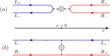
Figure 1: Schematic setup. (a) Semi-infinite left/right ($j=L/R$, blue/red) superconducting leads at $x<0/x>0$, respectively, harbor one-dimensional (1D) right ($+$) and left ($-$) movers and are tunnel coupled (dashed lines) to an Anderson dot (shaded circle) at $x=0$. (b) Unfolded representation with 1D chiral fermions.

Model.—We start with an Anderson dot tunnel-coupled to left/right superconducting leads ($j=L/R$), see Fig. 1(a). Writing $H=H_{d}+H_{t}+H_{\rm leads}$ with $H_{d}=\varepsilon_{d}(n_{\uparrow}+n_{\downarrow})+Un_{\uparrow}n_{\downarrow}$, where $n_{\sigma}=d_{\sigma}^{\dagger}d_{\sigma}$ for dot fermions $d_{\sigma}$, we have an interacting ($U>0$) dot level at energy $\varepsilon_{d}$. For simplicity taking identical dot-lead tunnel couplings ($t_{0}$), the point-like tunneling Hamiltonian is $H_{t}=t_{0}\sum_{\sigma}d_{\sigma}^{\dagger}b_{\sigma}(0)+{\rm h.c.}$, with symmetric combinations $b_{\sigma}(x)$ of 1D left/right lead fermion operators, cf. Eq. (2) below. Finally, $H_{\rm leads}$ describes $s$-wave BCS superconductor leads Altland2010 . Each semi-infinite lead supports right- and left-movers, $\psi_{j,\sigma}^{(\pm)}(x)\sim e^{\pm ik_{F}x}$. In the equivalent unfolded representation in Fig. 1(b), we have infinite chiral leads containing only left/right-moving field operators $\psi_{j,\sigma}(x)$ for lead $j=L/R$, respectively, $\psi^{(\pm)}_{L,\sigma}(x<0)=e^{\pm ik_{F}x}\psi_{L,\sigma}(\mp x)$ and $\psi^{(\pm)}_{R,\sigma}(x>0)=e^{\pm ik_{F}x}\psi_{R,\sigma}(\pm x)$. To simplify notation, we take the same absolute value $\Delta$ of the superconducting gap on both sides and put $\hbar=e=v_{F}=k_{B}=1$ (the normal density of states is then just $1/\pi$), resulting in

$$H_{\rm leads} = \sum_{j=L/R=\pm}\int_{-\infty}^{\infty}dx\Biggl{[}\sum_{\sigma=\uparrow,\downarrow}\psi^{\dagger}_{j,\sigma}\left(\pm i\partial_{x}\right)\psi_{j,\sigma}$$ (1)

$$+ \Delta\left(e^{\mp i\phi/2}\psi_{j,\downarrow}(x)\psi_{j,\uparrow}(-x)+{\rm h.c.}\right)\Biggr{]},$$

where $\phi$ is the phase difference. Next we switch to the linear combinations

$$\left\{\begin{array}[]{c}a_{\sigma}(x)\\ b_{\sigma}(x)\end{array}\right\}=\frac{1}{\sqrt{2}}\left[\psi_{L,\sigma}(-x)\mp\psi_{R,\sigma}(x)\right],$$ (2)

representing incoming (outgoing) fermion states for $x<0$ ($x>0$). The $a$-modes obey open boundary conditions corresponding to $a_{\sigma}(0^{+})=a_{\sigma}(0^{-})$, which for $t_{0}=0$ also apply to $b$-modes.

In the magnetic regime, $U\gg\max(\Delta,|t_{0}|^{2})$ and $-U<\varepsilon_{d}<0$, the impurity corresponds to a spin-$1/2$ operator ${\bf S}$, with the particle-hole symmetric Kondo limit at $\varepsilon_{d}=-U/2$. A Schrieffer-Wolff transformation yields $H\to H_{\rm leads}+H_{\rm K}$, where $H_{\rm K}$ contains a potential scattering term (for $\varepsilon_{d}\neq-U/2$) and an exchange term with coupling $J>0$ between ${\bf S}$ and the spin density of $b$-fermions at $x=0$ Hewson . Importantly, $a$-modes always decouple from the impurity and thus can be integrated out exactly. Using the imaginary-time functional integral approach Altland2010 , $b$-modes are then governed by the action $S_{b}+\int d\tau H_{\rm K}(\tau)$, where $S_{b}=-\sum_{k,\omega}\,\tilde{\Psi}^{\dagger}(k,\omega)G^{-1}(k,\omega)\tilde{\Psi}(k,\omega)$ with fermion Matsubara frequencies $\omega$ and the Nambu spinor

$$\Psi(x,\tau)=\left(\begin{array}[]{c}b_{\uparrow}(x,\tau)\\ b^{\dagger}_{\downarrow}(-x,\tau)\end{array}\right)\sim\sum_{k,\omega}e^{i(kx-\omega\tau)}\tilde{\Psi}(k,\omega).$$ (3)

Here and below, $\tilde{\Psi}(\omega)$ refers to the frequency representation of a time-dependent spinor $\Psi(\tau)$. After taking into account the pairing-induced bulk coupling between $a$ and $b$ fermions, the free ($t_{0}=0$) Green’s function (GF) appearing in $S_{b}$ is given by [cf. Eq. (1)],

$$G(k,\omega)=-\frac{i\omega+k\tau_{z}+\Delta\cos(\phi/2)\tau_{x}}{k^{2}+\omega^{2}+\Delta^{2}},$$ (4)

where Pauli matrices $\tau_{x,z}$ act in Nambu space.

Weak-coupling regime.—At high energy scales, the dynamics is restricted to the Hilbert subspace respecting open boundary conditions. Integrating also over the bulk $b_{\sigma}(x\neq 0)$ modes, we obtain $S_{b}=-\sum_{\omega}\tilde{\Psi}^{\dagger}(\omega)G^{-1}_{0}(\omega)\tilde{\Psi}(\omega)$ with $\Psi(\tau)=\Psi(0,\tau)$ and

$$G_{0}(\omega)=\int\frac{dk}{2\pi}\,G(k,\omega)=-\frac{i\omega+\Delta\cos(\phi/2)\tau_{x}}{2\sqrt{\omega^{2}+\Delta^{2}}}.$$ (5)

Standard energy-shell integration Altland2010 then yields the one-loop RG equations

$$\frac{dJ}{d\ell}=\frac{J^{2}}{\pi\sqrt{1+\delta^{2}}},\quad\frac{d{\cal Q}}{d\ell}=-\frac{3}{4\pi}\frac{\delta\cos(\phi/2)}{\sqrt{1+\delta^{2}}}J^{2},$$ (6)

where $\delta(\ell)=\Delta/D(\ell)$. As the effective bandwidth $D(\ell)=e^{-\ell}D$ decreases with increasing RG flow parameter $\ell$, a local pairing term, $H_{\rm AR}={\cal Q}b_{\downarrow}(0)b_{\uparrow}(0)+{\rm h.c.}$, is generated by AR processes. In fact, for $\phi\neq\pi$ (mod $2\pi$), the growing exchange coupling $J(\ell)$ drives ${\cal Q}(\ell)$ toward strong coupling, resulting in Kondo-enhanced AR Sand-Jespersen2007 ; Andersen2011 . Note that ${\cal Q}(\ell)\sim\cos(\phi/2)$ throughout the flow. However, the RG approach breaks down at energies below $T_{K}\simeq De^{-\pi/J}$, where one enters the strong-coupling regime.

Strong-coupling theory.—In the deep Kondo regime, the impurity spin is almost perfectly screened by the leads. To implement the Fermi liquid approach for the normal case, it is convenient to employ a scattering state formalism where the leading effects due to the polarizable Kondo singlet come from energy-dependent phase shifts and residual interaction corrections Nozieres1974 ; Gogolin2006 ; Sela2006 ; Mora2015 . For the superconducting case, we also need to include AR processes. This is achieved below by describing both AR and elastic scattering in a unified manner through a simple yet general boundary condition. To that end, by performing a Wick rotation, $i\omega\rightarrow E$, with energy $E$ relative to the chemical potential $\mu$, we define $\tilde{\Psi}_{\pm}(E)=\tilde{\Psi}(x=0^{\pm},E)$ from the Nambu spinor (3) taken at $x=0^{\pm}$. Arbitrary elastic scattering and AR processes are then captured by the boundary condition

$$\tilde{\Psi}_{+}(E)=e^{2i\hat{\eta}(E)}\tilde{\Psi}_{-}(E),\quad\hat{\eta}(E)=\left(\begin{array}[]{cc}\eta_{\uparrow}(E)&\eta_{a}(E)\\ -\eta_{a}^{\ast}(E)&\eta_{\downarrow}(-E)\end{array}\right),$$ (7)

where the Nambu matrix $\hat{\eta}(E)$ has the most general form allowed by Hermiticity of the self-energy $\hat{\Sigma}(E)$ in Eq. (8) below. While the real functions $\eta_{\uparrow,\downarrow}(E)$ are energy-dependent phase shifts precisely as in the normal case, the complex-valued function $\eta_{a}(E)$ describes AR.

Next, Eq. (7) is linked to the retarded response of bulk modes, $\tilde{\Psi}_{\pm}(E)=\sum_{k}e^{ik0^{\pm}}G^{R}(k,E)\tilde{\Psi}(E)$, to an effective boundary field, $\tilde{\Psi}(E)$, living at $x=0$. Using the retarded GFs $G^{R}(k,E)$ and $G^{R}_{0}(E)$ obtained by Wick rotation from Eqs. (4) and (5), respectively, we find $\tilde{\Psi}_{\pm}(E)=\left(G_{0}^{R}(E)\mp\frac{i}{2}\tau_{z}\right)\tilde{\Psi}(E).$ Here the $\tau_{z}$ term originates from the respective $\tau_{z}$ term in Eq. (4). One can thereby write Eq. (7) as equation of motion for the boundary spinor,

$$\left[G_{0}^{R}(E)+\hat{\Sigma}(E)\right]\tilde{\Psi}(E)=0,\quad\hat{\Sigma}(E)=\frac{1}{2}\cot[\hat{\eta}(E)]\tau_{z}.$$ (8)

Finally passing back to imaginary time and rescaling $\Psi(\tau)=\frac{1}{\sqrt{2}}\left(b_{\uparrow}(\tau),b^{\dagger}_{\downarrow}(\tau)\right)^{T}$, the strong-coupling action is given by [cf. Eqs. (5) and (8)]

$$S_{\rm sc}[\Psi] = -\sum_{\omega}\tilde{\Psi}^{\dagger}(\omega){\cal G}^{-1}(\omega)\tilde{\Psi}(\omega)+S_{I},$$ (9)

$${\cal G}^{-1}(\omega) = {\cal G}_{0}^{-1}(\omega)-\cot[\hat{\eta}(i\omega)]\tau_{z},\quad{\cal G}_{0}^{-1}(\omega)=-2G_{0}(\omega),$$

while $S_{I}$ describes residual interaction corrections addressed below. We emphasize that our self-energy formulation of AR and elastic scattering processes in Eq. (9) is completely general.

In order to arrive at a low-energy Fermi liquid theory, we now expand $\hat{\eta}(E)$ in powers of $|E|/T_{K}\ll 1$ and $\Delta/T_{K}\ll 1$. Using the spin symmetry of the problem and noting that conventional even-frequency pairing generated from Eq. (1) implies $\eta_{a}(-E)=\eta_{a}(E)$, we find

$$\eta_{\uparrow}(E) = \eta_{\downarrow}(E)=\eta_{F}+\alpha_{1}E+\alpha_{2}E^{2}+\cdots,$$ (10)

$$\eta_{a}(E) = \Delta\left(\beta_{1}+\beta_{3}E^{2}+\cdots\right),$$

where $\eta_{F}$ is the quasiparticle phase shift at the Fermi energy for $\Delta=0$. The Fermi liquid parameters $\alpha_{n}$ and $\beta_{n}$ scale as $1/T_{K}^{n}$, where the $\alpha_{n}$ determine the elastic scattering phase shifts Nozieres1974 ; Mora2015 and the complex-valued $\beta_{n}$ depend on the phase difference $\phi$ (see below). Keeping all terms up to order $1/T_{K}^{2}$, and using the renormalized parameters $\tilde{\alpha}_{n}=\alpha_{n}/\sin^{2}\eta_{F}$ and $\tilde{\beta}_{n}=\beta_{n}/\sin^{2}\eta_{F}$, we arrive at

$${\cal G}^{-1}(\omega) = {\cal G}_{0}^{-1}(\omega)-\left(\begin{array}[]{cc}\lambda(\omega)-i\tilde{\alpha}_{1}\omega&\tilde{\beta}_{1}\Delta\\ \tilde{\beta}_{1}^{\ast}\Delta&-\lambda(\omega)-i\tilde{\alpha}_{1}\omega\end{array}\right),$$ (13)

$$\lambda(\omega) = \cot\eta_{F}\left(1-\frac{\alpha_{1}^{2}\omega^{2}+|\beta_{1}|^{2}\Delta^{2}}{\sin^{2}\eta_{F}}\right)+\tilde{\alpha}_{2}\omega^{2}.$$ (14)

Further simplifications arise in the Kondo limit, where particle-hole symmetry (which is not broken by pairing terms) imposes the condition $\tau_{x}e^{2i\hat{\eta}(E)}\tau_{x}=e^{-2i\hat{\eta}(E)}$ SM , resulting in $\eta_{F}=\pi/2$, $\alpha_{2}=0$, and $\beta_{1}=\beta^{*}_{1}$. In the Kondo limit, we thus have $\lambda(\omega)=0$ in Eq. (14).

Residual interaction processes.—We now turn to $S_{I}$ in Eq. (9). Keeping all terms up to order $1/T_{K}^{2}$, this action contribution has the general form

$$S_{I}=\frac{1}{2}\sum_{\sigma=\uparrow,\downarrow}\int d\tau\ b^{\dagger}_{-\sigma}b_{-\sigma}b^{\dagger}_{\sigma}\left(\tilde{u}_{1}-\tilde{u}_{2}\partial_{\tau}\right)b_{\sigma},$$ (15)

with expansion parameters $\tilde{u}_{n}\sim 1/T_{K}^{n}$ (where $\tilde{u}_{1}\geq 0$). Defining normal ordering and averages $\langle\cdots\rangle_{0}$ with respect to the BCS ground state for ${\cal G}_{0}(\omega)$, cf. Eq. (9), it is convenient to express Eq. (15) by virtue of Wick’s theorem as $S_{I}=\langle S_{I}\rangle_{0}+\tilde{S}_{I}+S_{I}^{H},$ where $\tilde{S}_{I}$ is the normal-ordered form of Eq. (15) and $S_{I}^{H}$ represents Hartree terms which can be accounted for via the $\hat{\eta}(E)$-expansion in Eq. (10). Up to order $1/T_{K}^{2}$, with $u_{n}=\tilde{u}_{n}\sin^{2}\eta_{F}$, we find

$$\eta_{\sigma}(E) = \eta_{F}+\alpha_{1}E+\alpha_{2}E^{2}-\left(u_{1}+u_{2}E\right)\delta N_{-\sigma},$$

$$\eta_{a}(E) = \beta_{1}\Delta+u_{1}\delta Q,$$ (16)

where $\delta N_{\sigma}$ and $\delta Q$ are self-consistent Hartree parameters for local density and pairing fluctuations, respectively. Again invoking spin symmetry, $\delta N_{\uparrow}=\delta N_{\downarrow}$, Eq. (16) implies that Hartree terms can indeed be included by renormalizing $\alpha_{n}$ and $\beta_{n}$. We assume henceforth that this renormalization has already been carried out. Moreover, since the Kondo singularity is tied to the Fermi level, the phase shifts $\eta_{\sigma}(E)$ must be independent of the chemical potential $\mu$ Nozieres1974 ; Mora2015 . This fact implies that one can derive relations between Fermi liquid parameters without having to specify $\delta N_{\sigma}$ or $\delta Q$ Nozieres1974 ; Mora2015 . In particular, in the Kondo limit, $\partial_{\mu}\eta_{F}=0$ and $\alpha_{2}=u_{2}=0$ imply the well-known identity $u_{1}=\pi\alpha_{1}$ Nozieres1974 and $\partial_{\mu}\alpha_{1}=0$.

Current-phase relation.—The CPR follows as phase derivative of the free energy,

$$I(\phi)=2\partial_{\phi}F=I_{A}(\phi)+I_{\rm int}^{(1)}(\phi)+I_{\rm int}^{(2)}(\phi),$$ (17)

where $I_{A}(\phi)=-2T\sum_{\omega}\partial_{\phi}\ln\det{\cal G}^{-1}(\omega)$ is the Andreev bound state (ABS) contribution, see Eq. (14). In particular, the ABS spectrum follows by solving det$[{\cal G}^{-1}(-iE)]=0$ for subgap energies, $|E|<\Delta$. Keeping terms up to order $1/T_{K}$, where $\lambda(-iE)=\lambda=\cot\eta_{F}$ [cf. Eq. (14)], this condition reads

$$\frac{E^{2}}{\Delta^{2}}=\frac{\left|\cos(\phi/2)-\tilde{\beta}_{1}\sqrt{\Delta^{2}-E^{2}}\right|^{2}+\lambda^{2}}{\left(1+\tilde{\alpha}_{1}\sqrt{\Delta^{2}-E^{2}}\right)^{2}+\lambda^{2}}.$$ (18)

In the Kondo limit (with $\lambda=0$), Eq. (18) holds up to order $1/T_{K}^{2}$.

The leading interaction contribution to the CPR, see Eq. (17), follows from $\langle S_{I}\rangle_{0}$ SM ,

$$I^{(1)}_{\rm int}(\phi)=\delta I_{c}\sin\phi,\quad\delta I_{c}\simeq-\frac{\tilde{u}_{1}\Delta^{2}}{4\pi^{2}}\ln^{2}\left(T_{K}/\Delta\right).$$ (19)

As expected in the presence of repulsive quasiparticle interactions, we obtain a decrease of the critical current, $\delta I_{c}<0$, where $|\delta I_{c}|\sim\frac{\Delta^{2}}{T_{K}}\ln^{2}(T_{K}/\Delta)$ contains a logarithmic enhancement factor. Finally, $I_{\rm int}^{(2)}$ describes higher-order interaction corrections to the CPR due to $\tilde{S}_{I}$. To order $1/T_{K}^{2}$, we obtain SM

$$I^{(2)}_{\rm int}(\phi)\approx\tilde{u}_{1}^{2}\Delta^{3}\left(\sin\phi+\frac{1}{2}\sin(2\phi)\right),$$ (20)

where the $\sin(2\phi)$ term describes coherent tunneling processes involving two Cooper pairs.

Let us then turn to the dominant ABS contribution, see Eq. (18), where the $\phi$-dependence of the AR coupling $\tilde{\beta}_{1}$ follows from Eq. (6), $\tilde{\beta}_{1}(\phi)=\gamma\cos(\phi/2),$ with constant $\gamma\sim 1/T_{K}$. (i) For $T_{K}/\Delta\to\infty$, all Fermi liquid parameters and thus also the interaction corrections (19) and (20) can be dropped. Solutions to Eq. (18) are then given by $E=\pm\Delta\sqrt{1-{\cal T}\sin^{2}(\phi/2)}$ with the junction transparency ${\cal T}=\sin^{2}\eta_{F}=1/(1+\lambda^{2})$. We thus readily recover the results of Ref. Glazman1989 . (ii) Including $1/T_{K}$ corrections, see Fig. 2, Eq. (18) predicts a $4\pi$ periodic ABS spectrum in the Kondo limit ($\lambda=0$), with zero-energy ABS crossings at $\phi=\pi\leavevmode\nobreak\ ({\rm mod}\leavevmode\nobreak\ 2\pi$). For $\lambda\neq 0$, we instead have avoided crossings with gap $E_{g}\simeq 2\sqrt{1-{\cal T}}\Delta$, and thus obtain a conventional $2\pi$ periodic spectrum. (iii) Fermi liquid corrections imply a detachment of ABSs from quasiparticle continuum states at $\phi=0\leavevmode\nobreak\ ({\rm mod}\leavevmode\nobreak\ 2\pi)$. The detachment gap, $\delta_{A}=\Delta-E_{A}(0)$, follows from Eq. (18) as

$$\delta_{A}=2\sin^{4}(\eta_{F})\Delta^{3}\left[\tilde{\alpha}_{1}+{\rm Re}(\gamma)\right]^{2}\sim\frac{\Delta^{3}}{T_{K}^{2}}.$$ (21)

While ABS detachment already arises from elastic scattering Yeyati2003 , AR and Hartree corrections can strongly renormalize $\delta_{A}$. Since the Kondo resonance floats with the Fermi level and the ABS spectrum is detached from the continuum, the $4\pi$ periodic CPR in the Kondo limit should be observable for $T\ll\delta_{A}$.

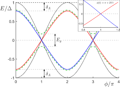
Figure 2: ABS spectrum vs phase $\phi$. Main panel: Black dotted curves show the particle-hole symmetric limit with $T_{K}/\Delta\to\infty$ Glazman1989 . Blue and red solid curves depict $4\pi$ periodic Andreev levels for $T_{K}/\Delta=5,\lambda=0$, and $\alpha_{1}=\gamma=1/T_{K}$. Green dashed curves illustrate the gap $E_{g}$ formed away from particle-hole symmetry ($\lambda=0.2$), leading to $2\pi$ periodicity. Inset: Asymmetry of $4\pi$-periodic adiabatic Andreev levels near the crossing at $\phi=\pi$ with voltage $V=0.33\Delta$ and ${\rm Im}(\gamma)=3/T_{K}$.

ABS spectrum for small voltage $V$.—What will happen to the $4\pi$ periodic Andreev spectrum in the Kondo limit when a small bias voltage $V$ is applied? For $V\ll\delta_{A}\ll\Delta$, adiabatic Andreev levels still represent good dynamical variables. Since the ABSs are removed from continuum states by a spectral gap, the retarded and advanced sectors of the Keldysh action decouple Altland2010 ; SM . To investigate whether the $4\pi$ periodicity survives in the nonequilibrium case, we consider the phase dynamics, $\phi(t)=\pi+2Vt$, at times where $\phi(t)\approx\pi\leavevmode\nobreak\ ({\rm mod}\leavevmode\nobreak\ 2\pi)$, corresponding to zero-energy crossings. The retarded sector can equivalently be described SM by the real-time action

$$S=\int dt\ \Phi^{\dagger}(t)\left[i\partial_{t}-E_{A}(t)\left(\sigma_{z}-\xi(t)\right)\right]\Phi(t),$$ (22)

where $\Phi=(c_{+},c_{-})^{T}$ contains the amplitudes for upper/lower ($\nu=+/-$) Andreev branches, the Pauli matrix $\sigma_{z}$ acts in Andreev level space, and

$$E_{A}(t)\simeq\frac{1-{\rm Re}(\gamma)\Delta}{1+\alpha_{1}\Delta}\ \Delta\sin(Vt).$$ (23)

In the near-adiabatic regime, the ABS degeneracy at each crossing is not lifted by the voltage, and the Andreev spectrum remains $4\pi$ periodic. We find $\xi(t)=\frac{1}{2}{\rm Im}(\gamma)V\cos(Vt)$ in Eq. (22), where ${\rm Im}(\gamma)\neq 0$ requires that particle-hole symmetry has been broken, e.g., by the voltage. The only effect of $\xi(t)$ then consists of an asymmetric distortion of the $\nu=+/-$ Andreev levels, cf. Eqs. (22), (23) and inset of Fig. 2,

$$\nu E_{A}\to\nu(1-\nu\xi)E_{A}.$$ (24)

Since $\xi\to-\xi$ at each subsequent crossing ($\phi\to\phi+2\pi$), Eq. (24) implies an asymmetric absorption and/or emission spectrum near the ABS crossings. Importantly, this feature allows one to experimentally distinguish the predicted $4\pi$ Josephson effect from its topological counterpart in Majorana junctions Alicea2012 ; Leijnse2012 ; Beenakker2013 as well as from other proposed realizations Kwon2004 ; Michelsen2008 ; Chiu2018 . The real and imaginary parts of $\gamma$ can be measured via the detachment gap $\delta_{A}$ [Eq. (21)] in the equilibrium Andreev spectrum and via the low-voltage asymmetry $\xi$, see Eq. (24), respectively.

Conclusions.—In this work, we have presented a Fermi liquid approach to the Kondo problem in a conventional $s$-wave BCS superconductor with $T_{K}\gg\Delta$. While we have illustrated the theory for an Anderson dot between two superconducting leads in the (near) equilibrium regime, the Fermi liquid description also allows to tackle many other setups featuring an interplay of Kondo physics with superconductivity.

Supplemental Material to “Fermi liquid approach for superconducting Kondo problems”

We here provide details about particle-hole symmetry constraints as well as short derivations of Eqs. (16), (17) and (19) quoted in the main text.

.1 Particle-hole symmetric Kondo limit

First we address the derivation of the relation

$$\tau_{x}e^{2i\hat{\eta}(E)}\tau_{x}=e^{-2i\hat{\eta}(E)},$$ (S1)

which holds in the particle-hole (PH) symmetric Kondo limit of the Anderson model with $\hat{\eta}(E)$ in Eq. (7) of the main text. The PH transformation ${\cal P}$ amounts to exchanging $\tilde{b}_{\sigma}(x,E)\leftrightarrow\tilde{b}^{\dagger}_{-\sigma}(x,-E)$ such that ${\cal P}\tilde{\Psi}_{\pm}(E)=\tau_{x}\tilde{\Psi}_{\mp}(E).$ By virtue of the relation

$$\tau_{x}\left[G_{0}^{R}(E)\mp\frac{i}{2}\tau_{z}\right]\tau_{x}=G_{0}^{R}(E)\pm\frac{i}{2}\tau_{z},$$

we find that the bulk action is ${\cal P}$-invariant. Concerning the boundary condition [cf. Eq. (7) in the main text], ${\cal P}$-invariance implies the condition ${\cal P}\tilde{\Psi}_{+}(E)=e^{2i\hat{\eta}(E)}{\cal P}\tilde{\Psi}_{-}(E).$ Hence we obtain Eq. (S1).

.2 Interaction corrections

Here we give additional details on the derivation of Eqs. (16) and (17) in the main text, where the leading interaction contributions $I^{(1)}_{\rm int}(\phi)$ and $I^{(2)}_{\rm int}(\phi)$, respectively, have been specified. First, the anomalous Hartree contribution to $\langle S_{I}\rangle_{0}$ follows from

$$\langle b_{\downarrow}(\tau)b_{\uparrow}(0)\rangle_{0} \simeq \frac{\Delta\cos(\phi/2)}{2\pi}\int_{0}^{T_{K}}\frac{d\omega}{\sqrt{\omega^{2}+\Delta^{2}}}$$ (S2)

$$\simeq \frac{\Delta\cos(\phi/2)}{2\pi}\ln(T_{K}/\Delta).$$

The corresponding free energy contribution from $\langle S_{I}\rangle_{0}$ is then given by

$$F^{(1)}_{\rm int}(\phi)=\tilde{u}_{1}(\Delta/2\pi)^{2}\ln^{2}(T_{K}/\Delta)\cos^{2}(\phi/2)$$ (S3)

and yields Eq. (16) in the main text. Second, higher-order corrections follow by cumulant expansion in $\tilde{S}_{I}$,

$$e^{-F^{(2)}_{\rm int}/T}=\left\langle{\cal T}_{\tau}e^{-\tilde{S}_{I}}\right\rangle=\exp\left(\frac{1}{2}\langle\tilde{S}_{I}^{2}\rangle_{c}+\cdots\right),$$ (S4)

where $\langle\cdots\rangle_{c}$ indicates that only connected diagrams are included and ${\cal T}_{\tau}$ is the imaginary-time ordering operator. To order $1/T_{K}^{2}$, we find from Eq. (S4) the contribution

$$F^{(2)}_{\rm int}=-\frac{T\tilde{u}_{1}^{2}}{2}\int_{0}^{1/T}d\tau_{1}d\tau_{2}\langle B(\tau_{1})B(\tau_{2})\rangle_{c}$$ (S5)

with $B(\tau)=b^{\dagger}_{\uparrow}(\tau)b_{\uparrow}(\tau)b^{\dagger}_{\downarrow}(\tau)b_{\downarrow}(\tau)$. Here $\phi$-dependent contributions mainly originate from the diagram with four anomalous contractions while the diagram with four normal contractions depends only weakly on $\phi$ and can be neglected. As a result, taking $T\to 0,$ we obtain

$$F^{(2)}_{\rm int} = -A\cos^{4}(\phi/2),$$ (S6)

$$A \simeq \tilde{u}_{1}^{2}\Delta^{3}\int_{0}^{\infty}d\xi\left(\int_{0}^{T_{K}/\Delta}dx\frac{\cos(x\xi)}{\pi\sqrt{1+x^{2}}}\right)^{4},$$

which yields Eq. (17) quoted in the main text.

.3 Adiabatic Andreev levels at small voltage

Consider the case of low bias voltage, $V\ll\delta_{A}\ll\Delta$, which implies a slowly varying phase difference, $\dot{\phi}(t)=2V$. The ABS occupation dynamics then stays almost all the time away from the gap edges such that the retarded and advanced sectors of the full Keldysh action are decoupled during the time evolution. The subgap dynamics is thus already described by an effective action for the retarded sector,

$$S=\int dtdt^{\prime}\Psi^{\dagger}_{q}(t){\cal L}(t,t^{\prime})\Psi_{c}(t^{\prime}),$$ (S7)

with

$${\cal L}(t,t^{\prime})=\frac{1}{2}\left(G_{+}+G_{-}\right)-\hat{\Sigma}.$$ (S8)

Here we have defined

$$G_{\pm}(t,t^{\prime})=e^{\pm i\tau_{z}\phi(t)/4}G_{0}^{R}(t-t^{\prime})e^{\mp i\tau_{z}\phi(t^{\prime})/4}$$ (S9)

and the Fourier transform of $G_{0}^{R}(t)$ is given by

$$G_{0}^{R}(E)=\frac{E+\Delta\tau_{x}}{\zeta_{E}},\quad\zeta_{E}=\sqrt{\Delta^{2}-(E+i0^{+})^{2}}.$$ (S10)

The Nambu spinors $\Psi_{c}$ and $\Psi^{\dagger}_{q}$ are the ’classical’ and ’quantum’ components of the boundary-field Keldysh spinor, respectively. For ease of notation, we drop the indices $(c,q)$ in what follows.

First, in the adiabatic approximation, one neglects $\dot{\phi}^{2}\sim V^{2}$, $\ddot{\phi}$, and all higher-order time derivatives. The GFs in Eq. (S9) then take the form

$$G_{\pm}(t,t^{\prime})\simeq$$ (S11)

$$\frac{1}{\zeta(t)}\left(\pm\frac{\dot{\phi}(t)}{4}\tau_{z}+i\partial_{t}+\Delta e^{\pm i\tau_{z}\phi(t)/2}\tau_{x}\right)\delta(t-t^{\prime}).$$

In addition, one puts $\zeta(t)=\sqrt{\Delta^{2}-E_{A}^{2}(t)}$ with the instantaneous ABS energy $E_{A}(t)\equiv E_{A}(\phi(t))$, where $E_{A}(\phi)$ solves the equilibrium condition in Eq. (15) of the main text. After rescaling $\Psi(t)\to\sqrt{\frac{\zeta(t)}{1+\tilde{\alpha}_{1}\zeta(t)}}\Psi(t),$ the effective action, $S=\int dt\Psi^{\dagger}(t){\cal L}(t)\Psi(t)$, has the time-local Lagrangian

$${\cal L}(t) = i\partial_{t}+\frac{\Delta}{1+\tilde{\alpha}_{1}\zeta(t)}\left[\cos\left(\frac{\phi(t)}{2}\right)\tau_{x}-\hat{\beta}_{1}(t)\zeta(t)\right]$$ (S12)

$$-\frac{\lambda\zeta(t)}{1+\tilde{\alpha}_{1}\zeta(t)}\tau_{z},$$

where $\hat{\beta}_{1}=\left(\begin{array}[]{cc}0&\tilde{\beta}_{1}\\ \tilde{\beta}_{1}^{\ast}&0\end{array}\right)$ and the time dependence of $\tilde{\beta}_{1}$ follows from the time dependence of the phase.

A systematic way to compute nonadiabatic corrections is to expand Eq. (S7) in powers of $\partial_{t}$,

$$S=\int dtd\tau\Psi^{\dagger}(t+\tau/2){\cal L}(t;\tau)\Psi(t-\tau/2),$$ (S13)

$${\cal L}(t+\tau/2,t-\tau/2)\equiv{\cal L}(t;\tau)=\int\frac{dE}{2\pi}\,e^{-iE\tau}{\cal L}(t;E),$$

where $t$ is the ’center-of-mass’ (and $\tau$ the relative) time. The Lagrangian, see Eq. (S8), in this mixed representation, ${\cal L}(t;E)$, involves the GF matrices [see Eq. (S9)]

$$G_{s=\pm}(t;E)=\frac{E+\tau_{z}sV/2}{\zeta_{E+\tau_{z}sV/2}}+\frac{\Delta}{\zeta_{E}}\left(\begin{array}[]{cc}0&e^{isVt}\\ e^{-isVt}&0\end{array}\right),$$ (S14)

and the self-energy part is given by

$$\hat{\Sigma}(t;E)\approx\lambda\tau_{z}-\tilde{\alpha}_{1}E+\Delta\left(\begin{array}[]{cc}0&\gamma\\ \gamma^{\ast}&0\end{array}\right)\cos(Vt).$$ (S15)

For a low-energy description, we neglect continuum states by projecting $\Psi(E)\rightarrow\Theta(\Delta-|E|)\Psi(E)$, which is justified for $|E\pm V/2|<\Delta$. We note that ${\cal L}(t;E)$ then also stays Hermitian. Since ${\cal L}(t;E)$ only slowly depends on $t$, to leading nontrivial order, the action is given by

$$S = \frac{1}{2}\int dt\Psi^{\dagger}(t)\left[{\cal L}(t;E)+\frac{i}{2}\partial_{t}\partial_{E}{\cal L}(t;E)\right]_{E=i\partial_{t}}\Psi(t)$$ (S16)

$$+{\rm h.c.},$$

where we neglect terms $\sim\partial_{t}^{n}{\cal L}(t;E)\propto V^{n}$ with $n\geq 2$.

We next introduce Nambu spinor eigenstates, $\chi_{\nu=\pm}(t)$, for instantaneous Andreev levels,

$${\cal L}(t;E=\nu E_{A}(t))\chi_{\nu}(t)=0,\quad\det\left[{\cal L}(t;E=\nu E_{A}(t))\right]=0,$$ (S17)

with $\chi^{\dagger}_{\nu}(t)\cdot\chi_{\nu^{\prime}}(t)=\delta_{\nu\nu^{\prime}}$. Expanding $\Psi(t)$ in this adiabatic Andreev basis,

$$\Psi(t)=\sum_{\nu=\pm}c_{\nu}(t)\chi_{\nu}(t)e^{-i\nu\int^{t}dsE_{A}(s)},$$ (S18)

and substituting Eq. (S18) into Eq. (S16), the effective action is written in terms of the amplitudes $c_{\nu}(t)$,

$$S = \frac{i}{2}\int dt\sum_{\nu,\nu^{\prime}=\pm}e^{i(\nu^{\prime}-\nu)\int^{t}dsE_{A}(s)}c_{\nu^{\prime}}^{\dagger}(t)\chi^{\dagger}_{\nu^{\prime}}(t)$$

$$\times \left[\partial_{E}{\cal L}(t;\nu E_{A})\partial_{t}+\frac{1}{2}\partial_{t}\partial_{E}{\cal L}(t;\nu E_{A})\right]c_{\nu}(t)\chi_{\nu}(t)+{\rm h.c.}$$

We now focus on the vicinity of the Kondo limit, where $\lambda=0$. However, $\beta_{1}$ can now be complex-valued since we allow for particle-hole symmetry breaking. In the mixed representation, cf. Eq. (S12), we find

$${\cal L}(t;E)=E+w_{E}\Delta\cos[\phi(t)/2]\left(\begin{array}[]{cc}0&e^{-i\theta_{E}}\\ e^{i\theta_{E}}&0\end{array}\right),$$ (S20)

where $w_{E}=\frac{\left|1-\gamma\zeta_{E}\right|}{1+\alpha_{1}\zeta_{E}}$ and $\theta_{E}=\tan^{-1}\frac{{\rm Im}(\gamma)\zeta_{E}}{1-{\rm Re}(\gamma)\zeta_{E}}$. We here assume $\phi(t)\equiv\pi+2Vt\approx\pi\,{\rm mod}(2\pi)$, i.e., we are near an ABS crossing. The adiabatic ABS energies follow as $E(t)=\pm w_{E}\Delta\sin(Vt)$, cf.  Eq. (20) of the main text. The corresponding eigenstates are $\chi_{\nu=\pm}(t)=(1,\nu e^{i\theta(t)})^{T}/\sqrt{2}$ with $\theta(t)=\theta_{E_{A}(t)}$. Substituting these expressions into Eq. (.3), computing the matrix elements between the states $\chi_{\nu}(t)$, and finally passing to the Heisenberg picture, $c_{\nu}(t)\to e^{i\nu\int^{t}dsE_{A}(s)}c_{\nu}(t)$, we arrive at the action specified in Eq. (19) of the main text.

References

(1)
A.C. Hewson, The Kondo Problem to Heavy Fermions (Cambridge University Press, Cambridge UK, 1993).
(6)
S. Nadj-Perge, I.K. Drozdov, J. Li, H. Chen, S. Jeon, J. Seo, A.H. MacDonald, B.A. Bernevig, and A. Yazdani, Science 346, 602 (2014).
(7)
M. Ruby, F. Pientka, Y. Peng, F. von Oppen, B.W. Heinrich, and K.J. Franke,
Phys. Rev. Lett. 115, 197204 (2015).
(8)
L.I. Glazman and K.A. Matveev, JETP Lett. 49, 659 (1989).
(9)
A.V. Rozhkov and D.P. Arovas, Phys. Rev. Lett. 82, 2788 (1999).
(10) Y. Avishai, A. Golub, and A.D. Zaikin, Phys. Rev. B 67, 041301(R) (2003).
(11)
E. Vecino, A. Martín-Rodero, and A. Levy Yeyati, Phys. Rev. B 68, 035105 (2003).
(12)
A. Levy Yeyati, A. Martin-Rodero, and E. Vecino, Phys. Rev. Lett. 91, 266802 (2003).
(13)
F. Siano and R. Egger, Phys. Rev. Lett. 93, 047002 (2004).
(14)
M.S. Choi, M. Lee, K. Kang, and W. Belzig, Phys. Rev. B 70, 020502 (2004).
(15)
G. Sellier, T. Kopp, J. Kroha, and Y.S. Barash, Phys. Rev. B 72, 174502 (2005).
(16)
F.S. Bergeret, A. Levy Yeyati, and A. Martín-Rodero, Phys. Rev. B 74, 132505 (2006).
(17) L. Dell’Anna, A. Zazunov, and R. Egger, Phys. Rev. B 77,
104525 (2008).
(18)
C. Karrasch, A. Oguri, and V. Meden, Phys. Rev. B 77, 024517 (2008).
(19)
T. Meng, S. Florens, and P. Simon, Phys. Rev. B 79, 224521 (2009).
(20)
B.M. Andersen, K. Flensberg, V. Koerting, and J. Paaske, Phys. Rev. Lett. 107, 256802 (2011).
(21)
A. Martín-Rodero and A.L. Yeyati, Adv. Phys. 60, 899 (2011).
(22)
D.J. Luitz, F.F. Assaad, T. Novotný, C. Karrasch, and V. Meden,
Phys. Rev. Lett. 108, 227001 (2012).
(23)
J.F. Rentrop, S.G. Jakobs, and V. Meden, Phys. Rev. B 89, 235110 (2014).
(24)
A.Y. Kasumov, R. Deblock, M. Kociak, B. Reulet, H. Bouchiat, I.I. Khodos, Y.B.
Gorbatov, V.T. Volkov, C. Journet, and M. Burghard, Science 284, 1508 (1999).
(25)
J.A. van Dam, Y.V. Nazarov, E.P.A.M. Bakkers, S. De Franceschi, and L.P. Kouwenhoven, Nature 442, 667 (2006).
(26)
J.P. Cleuziou, W. Wernsdorfer, V. Bouchiat, T. Ondarcuhu, and M. Monthioux, Nature Nanotech. 1, 53 (2006).
(27)
H. Ingerslev Jørgensen, T. Novotný, K. Grove-Rasmussen, K. Flensberg, and P.E. Lindelof, Nano Lett. 7, 2441 (2007).
(28)
T. Sand-Jespersen, J. Paaske, B.M. Andersen, K. Grove-Rasmussen, H.I. Jørgensen,
M. Aagesen, C.B. Sørensen, P.E. Lindelof, K. Flensberg, and J. Nygård,
Phys. Rev. Lett. 99, 126603 (2007).
(29)
A. Eichler, R. Deblock, M. Weiss, C. Karrasch, V. Meden, C. Schönenberger,
and H. Bouchiat, Phys. Rev. B 79, 161407 (2009).
(30)
R. Delagrange, D.J. Luitz, R. Weil, A. Kasumov, V. Meden, H. Bouchiat, and
R. Deblock, Phys. Rev. B 91, 241401 (2015).
(31)
P. Nozières, J. Low Temp. Phys. 17, 31 (1974).
(32)
A.O. Gogolin and A. Komnik, Phys. Rev. Lett. 97, 016602 (2006).
(33)E. Sela, Y. Oreg, F. von Oppen, and J. Koch, Phys. Rev. Lett. 97,
086601 (2006).
(34)
C. Mora, C. P. Moca, J. von Delft, and G. Zaránd, Phys. Rev. B 92, 075120 (2015).
(35)
C.P. Moca, C. Mora, I. Weymann, and G. Zaránd, Phys. Rev. Lett. 120, 016803 (2018).
(36)
A. Zazunov, R. Egger, and A. Levy Yeyati, Phys. Rev. B 94, 014502 (2016).
(37)
J. Alicea, Rep. Prog. Phys. 75, 076501 (2012).
(38)
M. Leijnse and K. Flensberg, Semicond. Sci. Techn. 27, 124003 (2012).
(39)
V. Mourik, K. Zuo, S.M. Frolov, S.R. Plissard, E.P.A. Bakkers, and L.P. Kouwenhoven,
Science 336, 1003 (2012).
(41)
A. Zazunov, F. Buccheri, P. Sodano, and R. Egger, Phys. Rev. Lett. 118, 057001 (2017).
(42)
S.M. Albrecht, A.P. Higginbotham, M. Madsen, F. Kuemmeth, T.S. Jespersen,
J. Nygård, P. Krogstrup,
and C.M. Marcus, Nature 531, 206 (2016).
(43)
E. Bocquillon, R.S. Deacon, J. Wiedenmann, P. Leubner, T.M. Klapwijk, C. Brüne, K. Ishibashi, H. Buhmann, and L.W. Molenkamp, Nat. Nanotechnol. 12, 137 (2017).
(44)
D. Laroche, D. Bouman, D.J. van Woerkom, A. Proutski, C. Murthy, D.I. Pikulin,
C. Nayak, R.J.J. van Gulik, J. Nygård, P. Krogstrup, L.P. Kouwenhoven, and
A. Geresdi, arXiv:1712.08459.
(45)
A. Fornieri, A.M. Whiticar, F. Setiawan, E.P. Marín, A.C.C. Drachmann,
A. Keselman, S. Gronin, C. Thomas, T. Wang, R. Kallaher, G.C. Gardner,
E. Berg, M.J. Manfra, A. Stern, C.M. Marcus, and F. Nichele, preprint arXiv:1809.03037.
(46) H.-J. Kwon, K. Sengupta, and V.M. Yakovenko, Eur. Phys. J. B 37, 349 (2004).
(47) J. Michelsen, V.S. Shumeiko, and G. Wendin, Phys. Rev. B 77, 184506 (2008).
(48) C.K. Chiu and S. Das Sarma, arXiv:1806.02224.
(49)
A. Altland and B.D. Simons, Condensed Matter Field Theory, 2nd ed. (Cambridge University Press, Cambridge, UK, 2010).
(50)
See the accompanying online Supplemental Material, where we provide details about particle-hole symmetry
constraints and short derivations of Eqs. (19), (20), and (22).