The young massive star cluster Westerlund 2 observed with MUSE.
I. First results on the cluster internal motion from stellar radial velocities

Abstract

Westerlund 2 (Wd2) is the central ionizing star cluster of the H II region RCW 49 and the second most massive young star cluster (${\rm M}=(3.6\pm 0.3)\times 10^{4}\,{\rm M}_{\odot}$) in the Milky Way. Its young age ($\sim 2\,$Myr) and close proximity to the Sun ($\sim 4\,$kpc) makes it a perfect target to study stars emerging from their parental gas cloud, the large number of OB-stars and their feedback onto the gas, and the gas dynamics. We combine high-resolution multi-band photometry obtained in the optical and near-infrared with the Hubble Space Telescope (HST), and VLT/MUSE integral field spectroscopy to study the gas, the stars, and their interactions, simultaneously. In this paper we focus on a small, $64\times 64\,{\rm arcsec}^{2}$ region North of the main cluster center, which we call the Northern Bubble (NB), a circular cavity carved into the gas of the cluster region. Using MUSE data, we determined the spectral types of 17 stars in the NB from G9III to O7.5. With the estimation of these spectral types we add 2 O and 5 B-type stars to the previously published census of 37 OB-stars in Wd2. To measure radial velocities we extracted 72 stellar spectra throughout Wd2, including the 17 of the NB, and show that the cluster member stars follow a bimodal velocity distribution centered around $(8.10\pm 1.53)\,{\rm km}\,{\rm s}^{-1}$ and $(25.41\pm 1.57)\,{\rm km}\,{\rm s}^{-1}$ with a dispersion of $(4.52\pm 1.78)\,{\rm km}\,{\rm s}^{-1}$ and $(3.46\pm 1.29)\,{\rm km}\,{\rm s}^{-1}$, respectively. These are in agreement with CO($J=1$–2) studies of RCW 49 leaving cloud-cloud collision as a viable option for the formation scenario of Wd2. The bimodal distribution is also detected in the Gaia DR2 proper motions.

1 Introduction

The young massive stars cluster (YMC) Westerlund 2 (Wd2, Westerlund, 1961) is the central ionizing cluster of the H II region RCW49 (Rodgers et al., 1960) and is the second most massive YMC in the Milky Way (MW, total stellar mass: $(3.6\pm 0.3)\times 10^{4}{\rm M}_{\odot}$, Zeidler et al., 2017) located in the Sagittarius spiral arm $\left(\alpha,\delta\right)=\left(10^{\rm h}23^{\rm m}58^{\rm s},-57^{\circ}45^{\prime}49^{\prime\prime}\right)$(J2000) (l,b)=$\left(284^{\circ}.3,-0^{\circ}.34\right)$. With its young age of $1-2$ Myr, its close proximity to the Sun (4.16 kpc, Vargas Álvarez et al., 2013; Zeidler et al., 2015), and its high-mass stellar content (37 spectroscopically identified OB-type stars, Moffat et al., 1991; Vargas Álvarez et al., 2013) it is a perfect testbed to study the early evolution and feedback of YMCs. Moffat et al. (1991) also suggests that Wd2 contains more than 80 O-type stars.

We have studied Wd2 photometrically using Hubble Space Telescope (HST) multi-band data (ID: 13038, PI: A. Nota) obtained in the optical and infrared (Zeidler et al., 2015, 2016, 2017) with the Advanced Camera for Surveys (ACS, Avila, 2017) and the infrared channel of the Wide Field Camera 3 (WFC3/IR, Dressel, 2018). In addition to the age and distance estimate, we confirmed the finding by Hur et al. (2015) that Wd2 consists of two sub-clumps (Zeidler et al., 2015), the main cluster (MC) and the northern clump (NC). Both clumps appear to be coeval. We derived a stellar mass function (MF) of the whole cluster area, as well as different sub regions (using elliptical annuli centered on the cluster center), and we showed that the high-mass slope of the MF is $\Gamma=-1.53\pm 0.05$, steeper than a Salpeter (1955) slope of $\Gamma=-1.35$. This is quite common among YMCs, e.g.: $\Gamma=-1.44^{+0.56}_{-0.08}$ for Westerlund 1 (Gennaro et al., 2011) or $\Gamma=-1.87\pm 0.41$ for NGC 346 (Sabbi et al., 2008). A study of the evolution of the MF slope with increasing radii from the cluster center revealed that Wd2 is highly mass segregated, and given the young age, the mass segregation is likely primordial.

Combining HST photometric wide and narrow-band filters, 240 bona-fide pre-main sequence (PMS) H$\alpha$ excess emitters were identified (Zeidler et al., 2016) indicating still ongoing mass accretion on the host stars. The analysis of the mass accretion hinted at an increase of the mass accretion rate with distance to the luminous OB stars. This suggests that the high amount of FUV flux radiated by the OB stars leads to a faster disk dispersal in close proximity to massive stars.

Studying Galactic YMCs spectroscopically has traditionally been challenging. Slit and fiber spectrographs only allow a very limited number of stars to be observed with a reasonable allocation of telescope time. This has changed in the past decade, when the development of integral field units (IFUs) has made major progress. Using the Multi Unit Spectrographic Explorer (MUSE, Bacon et al., 2010), mounted in the Nasmyth focus of UT4 at the Very Large Telescope (VLT) allows us, for the first time, to efficiently map Galactic star clusters spectroscopically. MUSE has a field-of-view (FOV) of $1~{}\rm{arcmin}^{2}$ at a spatial sampling of $0.2~{}\rm{arcsec~{}px}^{-1}$ and a resolving power of $R\approx 2000$–4000 at optical wavelengths between $4650\rm{\AA}$ and $9300\rm{\AA}$. This gives a total number of spectral pixels (spaxels) of $\sim 96000$ and $3800$ wavelength bins with $\Delta\lambda=1.25\rm{\AA}$. In the past, MUSE has been proven to be an excellent instrument to reveal motions, abundances, and 3D structures of gas and molecular clouds (e.g., the Pillars of Creation in M16 and the central Orion nebula, McLeod et al., 2015, 2016). In addition, MUSE has been used to measure the stellar radial velocities and velocity dispersions of, e.g., the globular cluster NGC 6397 (Kamann et al., 2016) or the ultra-faint stellar system Crater/Laevens I (Voggel et al., 2016).

In this paper we show that, in combination with high-resolution photometry from HST, MUSE is a powerful instrument to study both the stellar and gas content in YMCs and gives us the opportunity to estimate the velocity dispersion with a high enough accuracy to determine whether Wd2 is massive enough to be long-lived. If Wd2 is massive enough to survive the sudden changes in the gravitational potential, as soon as the massive OB star population explodes, this cluster may provide new insight to answer if YMCs are possible progenitors to globular clusters (e.g., Kruijssen, 2015). The stellar velocities shed light on the formation and history of Wd2 to see which cluster-formation theory applies: monolithic (e.g., Lada et al., 1984; Banerjee & Kroupa, 2015) or hierarchical (e.g., Parker et al., 2014) cluster formation, cloud-cloud collision (e.g., Nigra et al., 2008; Cignoni et al., 2009; Fukui et al., 2014), or even a combination of all three together.

This paper is structured as follows: In Sect. 2 we give an overview of the studied region. In Sect. 3 we introduce our dataset and the data reduction. In Sect. 4 we analyze the extracted spectra and describe the spectral typing. In Sect. 5 we describe the technique for measuring the radial velocities. In Sect. 6 we discuss our findings and compare results, while in Sect.7 we summarize our findings and provide a future outlook on this project.

2 The Northern Bubble

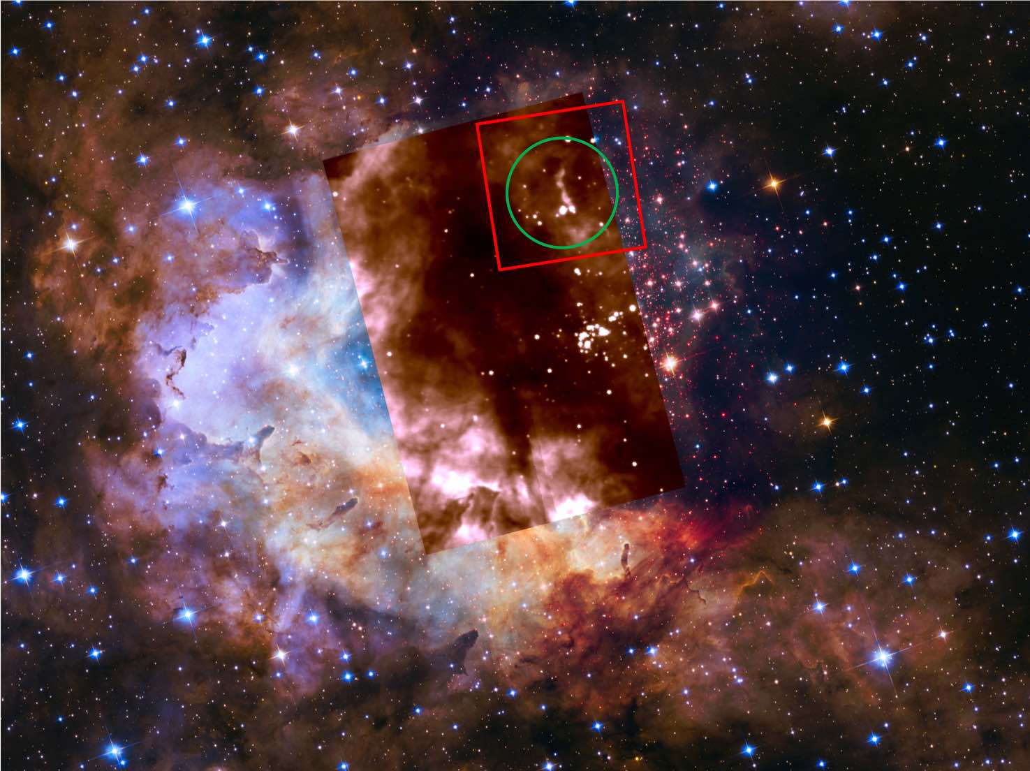
Figure 1: Color composite image of the HST ACS and WFC3/IR data of Wd2, including the $F125W$ (red), $F814W$ (green), and $F555$W (blue) filters. We present the mosaic of the 6 observed MUSE cubes (short exposures) as an inlay. The red box marks the $64^{\prime\prime}\times 64^{\prime\prime}$ NB region, while the green circle marks the NB. North is up, east to the left. HST image Credit: NASA, ESA, the Hubble Heritage Team (STScI/AURA), A. Nota (ESA/STScI), and the Westerlund 2 Science Team.

Hur et al. (2015), Zeidler et al. (2015), and Zeidler et al. (2017) pointed out that Wd2 is built up of two clumps, the Main Cluster (MC) and the Northern Clump (NC). The NC is located $\sim 1$pc North of the MC and has a photometric mass of $\left(3\pm 0.3\right)\cdot 10^{3}{\rm M}_{\odot}$. In this paper we mainly focus on a sub-region of our dataset covering the area around the NC forming a cavity in the gas distribution of the H II region (see Fig. 1 and Fig. 2). From now on we call this region the Northern Bubble (NB). In the center of this cavity lies a pillar or jet-like gas structure, which we refer to as ”the Sock”. The NB was first mentioned by Vargas Álvarez et al. (2013) as a ring-like structure. They suggested it to be the boundary of the H II-region surrounding a luminous O5V-III((f)) star (Fig 2 and Rauw et al., 2007). By looking at Spitzer images of this region, Vargas Álvarez et al. (2013) concluded that this ring ”is present in all IRAC bands but best seen at $[8.0]$, consistent with PAH emission from a photodissociation region”. This structure is thus representative of the physical interplay between massive stars and their surrounding ISM. The fact that it is characterized by a low stellar density (thus crowding effects are a lesser issue) makes it a perfect testbed for developing analysis routines, later applicable to the full dataset (see Sect. 3).

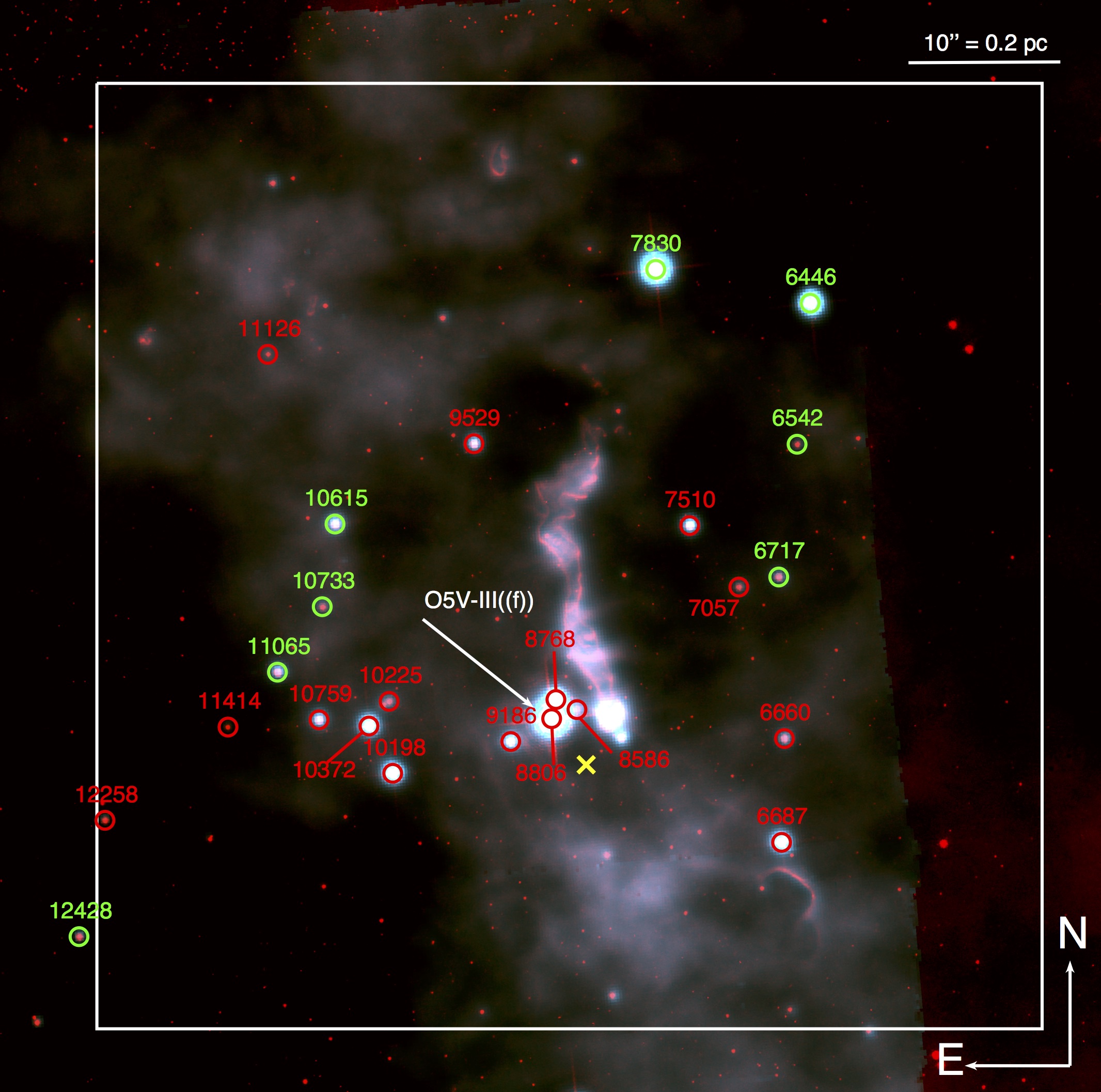
Figure 2: A color-composite image, representing emission in the HST H$\alpha$ ($F658N$ filter, red), N II 6583Å (green), and O III 5007Å (blue) filters, covering the $64^{\prime\prime}\times 64^{\prime\prime}$ field examined in this work (red square, see also Fig. 1). The HST H$\alpha$ is used to see small scale structure, below the resolution limit of MUSE, as well as faint stars. The yellow cross marks the center of the NC (Zeidler et al., 2017). The stars analyzed in this work are marked in red for NB members and in green for field stars. The numbers show the catalog identifier (see also Tab. 3).

3 Data reduction and source extraction

3.1 The observations

We observed Wd2 with MUSE in extended mode during the ESO period 97 (Program ID: 097.C-0044(A), PI: P. Zeidler). During the night of 2016, June 02/03, we acquired 6 pointings with 3 dither positions each for a total exposure time of $660~{}\rm{s}$. The dither pattern follows a 90 and 180 degrees rotation strategy to minimize detector defects and impurities. The observations were obtained in two observation blocks (OBs): 1323877 and 1323880. The seeing ranges from $0.61^{\prime\prime}-1.1^{\prime\prime}$ with an airmass of $1.21-1.28$ and $0.49^{\prime\prime}-0.78^{\prime\prime}$ with an airmass of $1.29-1.43$, respectively. A detailed overview of the data is presented in Zeidler & et (2018, in prep.). A second proposal has been approved and observed covering the whole Wd2 region, including some of the surrounding gas. In total we have obtained 15 pointings, including deep ($3\times 3600\,\rm{s}$) exposures to observe the PMS down to 1–2 M_⊙. We used the standard reduction pipeline (v.2.0.1) provided by ESO (Weilbacher et al., 2012, 2014) to reduce the data and combine the dither pattern into 6 data cubes (one for each pointing). This pipeline is based on the ESO Reflex environment (ESORex) for automated data reduction work flows for astronomy (Freudling et al., 2013). The datacubes are wavelength calibrated and the radial velocity of the telescope is corrected to the barycenter of the Solar System. We visually inspected the datacubes to determine that the different dither positions were properly aligned and that the data reduction was a success. The mosaic of the six data cubes is shown in Fig. 1 as an inlay in the HST color-composite image of the Wd2 region. The spatial sampling is $0.2^{\prime\prime}\,\rm{px}^{-1}$ with a spectral sampling of 1.25 Å, the resolution is 2.4 Å($\rm{R}\approx 2000$–4000 from blue to red).

3.2 The source extraction

Analyzing MUSE data obtained in crowded regions, such as YMCs, is challenging. We need to detect and mask stars in order to investigate the gas (e.g., McLeod et al., 2015) but for the stellar source extraction, a wavelength-dependent point spread function (PSF) and wavelength-dependent background have to be taken into account. This is done with ”PampleMuse”, a python package developed by Sebastian Kamann (Kamann et al., 2013) that uses a deep (at least 2 mag deeper than the detection limit of the MUSE observations), high-resolution photometric catalog to perform PSF spectrophotometry on the pipeline-reduced MUSE data cubes. In their study of simulated MUSE data of a crowded field, Kamann et al. (2013) showed that it is possible to extract $\sim 5000$ useful stellar spectra per arcmin². Here we give a short overview of the source extraction procedure. For a detailed description, see Zeidler & et (2018, in prep.):

• As first step, PampelMuse selects isolated (low crowding) bright sources to perform PSF spectrophotometry. This defines a wavelength-dependent PSF and corrects for a spatial offset or rotation with respect to the reference catalog and for wavelength-dependent variations in the positions.

• The wavelength-dependent PSF profile and coordinate corrections are then used for all of the stellar sources down to a signal-to-noise (S/N) based brightness limit. With this method sources separated less than their full-width half maximum (FWHM) can still be extracted.

• The background around each star is estimated by subdividing the FOV in sub-regions.

• The final products are background-subtracted spectra of the stars in the FOV.

From our parent sample that will be presented in Zeidler & et (2018, in prep.) and that contains all stars covered by the short and long exposures down to a ${\rm S/N}\approx 5$, we selected all stars in the NB with a ${\rm S/N}\geq 20$. In addition, we selected 55 stars with ${\rm S/N}\geq 20$ from the other parts of the MUSE mosaic to study the cluster dynamics.

4 The MUSE spectra

The background subtraction described in Sect. 3 works well for stars that are located in areas with a low background variability. If for example, a star is located in front of a gas ridge, the background emission coming from the gas is highly different on one side of the star compared to the other, which leads to a gradient in the background distribution. This becomes especially apparent at wavelengths where stars have absorption lines and the gas has strong emission lines (e.g,. hydrogen and helium lines), leading to either an over or under-subtraction of the background. We inspected the PampelMuse extracted spectra by eye and, as an indicator, we used the [N II]$\lambda\lambda 6549,6583$ lines to evaluate the quality of the background subtraction. These two lines are purely nebular lines and should totally disappear in the stellar spectra. In addition, we used strong lines, especially H$\alpha$ and H$\beta$, which often show negative fluxes in case of a background over-subtraction. With this method we selected those stars, for which we have spectra with a well-subtracted background.

4.1 Normalization and line identification

To normalize and rectify the extracted spectra we use the spectral fitting package pyspeckit. This python based routine allows us to fit spectral lines (absorption and emission) together with a continuum in an iterative process to determine an optimal solution. Due to the wavelength range of more than $4000~{}\rm{\AA}$ we split the wavelength range into 22 blocks to find a reliable continuum solution using low-degree polynomials.

To identify stellar spectral features, we used several sources in the literature, such as Gray & Corbally (2009, and references therein); Kaler (2011, and references therein); Rauw et al. (2011, and references therein); Sota et al. (2011, 2014, and references therein). To obtain the exact rest wavelengths of the absorption lines we used the ”NIST Atomic Spectra Bibliographic Databases”. For the identification of diffuse interstellar bands (DIBs) we used the ”DIB Database” and specifically the studies of the stellar spectrum of HD183143 by Hobbs et al. (2009).

The spectra of early-type stars (mostly O and B) are typically dominated by neutral and ionized helium lines, while common features of late-type stars are neutral and ionized metals and the pronounced Ca II-triplet, typical of cooler atmospheres.

4.2 Spectral Classification

To estimate the spectral type of each of the stars in our sample, we performed a multi-step classification. We sorted the stars in four major categories:

• Stars showing He I and He II absorption lines are classified as O-type stars.

• Stars showing He I but no He II are classified as B-type stars.

• Stars that show no helium lines but strong hydrogen lines, and a few ionized metals are classified as A-type stars.

• Stars showing the prominent Ca II-triplet and ionized and neutral metals are classified as A9 and later.

4.2.1 The O stars

The classification of O-type stars is usually done in the ultraviolet ($\lambda\leq 4600{\rm\AA}$, e.g., Walborn & Fitzpatrick, 1990). Since the MUSE spectra cover optical and NIR wavelengths, we used the empirical work of Kobulnicky et al. (2012). They used the equivalent width (EW) ratio of He II$\lambda 5411$ over He I$\lambda 5876$ and fitted it against the effective stellar temperature ($T_{\rm eff}$). This relation can be described with a $3^{\rm rd}$-order polynomial as derived by Vargas Álvarez et al. (2013):

$$\frac{{\rm EW}\left({\rm HeII}\lambda 5411\right)}{{\rm EW}\left({\rm HeI}\lambda 5876\right)} = 1.16208\times 10^{-12}\,T_{\rm eff}^{3}$$

$$-1.19205\times 10^{-7}\,T_{\rm eff}^{2} + 4.22137\times 10^{-3}\,T_{\rm eff}$$ (1)

$$- 50.5093.$$

The EWs are measured using pyspeckit. The transformation from temperature to spectral type is made using the calibrations of parameters for O-type stars by Martins et al. (2005), specifically:

$$T_{\rm eff}=50838-1995\times{\rm ST}.$$ (2)

The individual derived parameters of the found O-stars summarized in Tab. 1.

Table 1: The O-type stars

ID	EW(He I)	EW(He II)	$T_{\rm eff}$	spectral type	spec. mass
	[Å]		[K]		[M⊙]
10198	0.8201	0.4664	31884	O9.5	15.55
10372	0.8933	0.7374	33553	O8.5	18.80
8768	0.8352	1.0804	36155	O7.5	22.90
7510	0.6781	0.3010	31151	B0	$<15.55$

Note. — In this table we present the results and the spectral types of the O-type stars. In column 1 we give the stellar ID (as used in our HST photometric catalog, see Zeidler et al., 2015). In Columns 2 and 3 the measured EWs are presented, while in Columns 4–6 the resulting $T_{\rm eff}$, the spectral types, and the spectroscopic masses (provided by the models of Martins et al., 2005) are given, respectively. We note here that the spectroscopic masses have an uncertainty 35–50% (Martins et al., 2005).

4.2.2 The B stars

A similar relation can be found for B-type stars (see Fig. 4 of Kobulnicky et al., 2012) using the EW of He I and the ratio ${\rm EW}\left({\rm H}\alpha\right)/{\rm EW}\left({\rm HeI}\lambda 5876\right)$. For stars earlier than B3 this method becomes degenerate. Due to the insufficient accuracy of the results of the fitted parameters in Kobulnicky et al. (2012) we used the information given in that paper to perform our own fit with the following results:

$$\frac{{\rm EW}\left({\rm H}\alpha\right)}{{\rm EW}\left({\rm HeI}\lambda 5876\right)} = -1.27078\times 10^{-11}\,T_{\rm eff}^{3}$$

$$-9.17611\times 10^{-7}\,T_{\rm eff}^{2} - 2.18026\times 10^{-2}\,T_{\rm eff}$$ (3)

$$+ 173.99531,$$

$${\rm EW}\left({\rm HeI}\lambda 5876\right) = 2.91583\times 10^{-13}\,T_{\rm eff}^{3}$$

$$-2.12788\times 10^{-8}\,T_{\rm eff}^{2} + 5.12709\times 10^{-4}\,T_{\rm eff}$$ (4)

$$- 3.405698.$$

To estimate the spectral type from the effective temperature we used the results from Underhill et al. (1979). The relation ST- $\log(T_{\rm eff})$ is remarkably linear, which leads to ${\rm ST}=-8.56\times\log(T_{\rm eff})+88.02$. An overview of the determined spectral types can be found in Tab. 2.

Table 2: The B-type stars

ID	EW(He I)	EW(H$\alpha$)	$T_{\rm eff}$	spectral type
	[Å]		[K]
6687	0.7560	3.5973	24880	B1.5
9186	0.7485	4.0304	24540	B1.5
7510	0.6781	3.7377	28949	B0
9529	0.5445	4.0155	16149	B5
10759	0.6216	3.9803	17290	B4.5
6660	0.6640	3.6446	18490	B4.5
7057	1.0324	4.1731	18730	B4

Note. — In this table we present the spectral typing of the B-type stars. In column 1 we give the stellar ID (as specified in Zeidler et al. (2015)). In Columns 2 and 3 the measured EWs are presented, while in Columns 4 and 5 the resulting $T_{\rm eff}$, and the spectral types are given, respectively.

4.2.3 The late-type stars

For the stars with spectral type A9 or later, the Ca II-triplet is present. We used the Ca II-triplet libraries provided by Cenarro et al. (2001) and Munari & Tomasella (1999) together with the Penalized Pixel-Fitting (pPXF Cappellari & Emsellem, 2004; Cappellari, 2017) method to find the best-fitting template. We excluded the wavelength range between $8610{\rm\AA}$ and $8634{\rm\AA}$ due to a possible blend of the Fe I$\lambda 8622$ line with a DIB. We chose the best fitting model based on the $\chi^{2}$ value. For the ”traditional” spectral typing with by-eye inspection of the remaining stars we refer to the Appendix B. Both results, the individual by-eye inspection of the spectral lines and the cross-correlation of the spectra with template libraries are in good agreement, indicating that the automated, scripted method is reliable.

A summary of all the derived spectral types of all stars is given in Column 14 of Tab. 3.

4.2.4 Star #10225 - a peculiar object

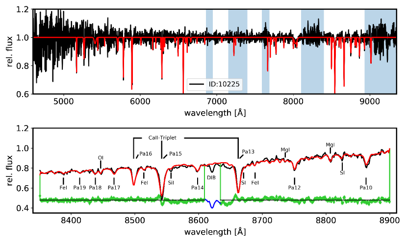
Figure 3: MUSE spectra for star #10225: The top panel shows the rectified spectrum with the fitted absorption lines in red. The estimated mass based on its location in the CMDs is $4.25~{}{\rm M}_{\odot}$. The bottom panel shows the Ca II-triplet region with the extracted spectrum in black and the best fitting template (Cenarro et al., 2001) in red. In green are marked the fit residuals. We marked the important lines used for the spectral typing. The DIB at $8620{\rm\AA}$ is also marked.

The spectrum of star #10225 is shown in Fig. 3. The weak Balmer lines (H$\beta$ disappears in the noise) suggest a spectral type of F or later. Despite the weak hydrogen lines, the Paschen (Pa)-series is visible up to the P18/19-lines suggesting this star is a giant or supergiant (luminosity class I or II). The lack of nitrogen lines in the Ca II-triplet region and the appearance of many neutral metals, such as Fe I, Si I, and Mg I (see bottom panel of Fig. 3) favors a G-type star. The best fitting template is the one of a G5Ib star, a yellow supergiant. The spectral type of a G5Ib star in combination with the photometric mass of $4.25\,{\rm M}_{\odot}$ (Zeidler et al., 2017) would suggest an age of 10–30 Myr, much older than the age of Wd2 ($\sim 2$ Myr). Although the location of a star in color-magnitude diagrams (CMDs) defines it as a cluster member, the selection based on photometry alone may be misleading. Wd2 is located in the MW disk and, therefore, foreground interlopers or highly reddened supergiants located behind the cluster are able to contaminate the PMS. Hur et al. (2015) estimated the probability for a field star contamination to be 2.8%, which is small but not impossible. While the high extinction caused by the H II region makes the scenario of a background source contaminating the cluster sequence basically impossible, foreground field stars are not excluded.

In the following we will discuss the two options: 1) the star is a G5 sub-giant occupying the same region of the CMD as Wd2’s PMS, and 2) the star is G5 PMS star:

1) The star is a G5 interloper: despite the low probability (2.8%, Hur et al., 2015), star #10225 might be a foreground sub-giant occupying the same locus in the CMD as the Wd2 PMS. Hur et al. (2015) argue that the maximum reddening of the foreground field stars does not exceed $E(B-V)_{\rm fg}=1.05\,{\rm mag}$ with an $R_{\rm V,fg}=3.33$ and a distance modulus of 11.8 mag. As a result, $A_{\rm V,fg}=R_{\rm V,fg}\times E(B-V)_{\rm fg}=3.50\,{\rm mag}$ is the maximum extinction correction that can be applied to any field star in front of Wd2. In Fig. 4 we show the $F814W-F160W$ vs. $F814W$ (left panel) and $F555W-F814W$ vs. $F555W$ (right panel) CMDs. The measured and foreground-extinction corrected positions of star #10225 and the reddening vector are indicated. In the $F814W-F160W$ vs. $F814W$ CMD the best-fitting stellar evolutionary track (blue line, Paxton et al., 2011, 2013, 2015; Choi et al., 2016; Dotter, 2016) represents a $1.1\,{\rm M}_{\odot}$ star and #10225 would be indeed a G5 sub-giant. In the $F555W-F814W$ vs. $F555W$ the same evolutionary track does not fit the locus of the star. A distance modulus of 14.4 mag ($d=6.6\,{\rm kpc}$) is necessary to fit the star. We also tested the scenario that there is a dust cloud located in front of this star, which changes the extinction law. To fit the star’s position to the evolutionary tracks in both CMDs an abnormal extinction law of $R_{\rm V}=2.45$, $E(B-V)_{\rm fg}=1.55\,{\rm mag}$ would be required (green star in Fig. 4). Therefore, we can conclude that star #10225 is not a foreground star.

2) The star is a G5 PMS star: under the assumption that this star is a cluster member the photometric mass is $4.25\,{\rm M}_{\odot}$ (Zeidler et al., 2017). The stellar evolutionary track for such a stellar mass (see green lines in Fig. 4) fits the locus of this star for both CMDs. Late-type PMS stars appear much brighter during their brief period on the turn-on compared to their MS life. This leads to the effect that a low-mass PMS star (green evolutionary track in Fig. 4) is similarly bright than a higher-mass early type star (yellow evolutionary track in Fig. 4), e.g., star #10759, which has been classified as a B4.5 star (see Sect. 4.2.2 and Tab. 3). Although their spectral types and masses are different (star #10759 has a photometric mass of $6.6\,{\rm M}_{\odot}$) their brightness only differs by 1.27 mag in $F555W$ and 0.93 mag in $F814W$. The misclassification of the spectral type as a G5Ib star may have happened due to ”veiling”. Veiling describes a reduction of the photospheric absorption lines by an accretion continuum in T-Tauri stars. Especially affected are hydrogen lines (e.g., Herczeg & Hillenbrand, 2014, and references therein), which increases the relative strength of the Ca II-triplet compared to the Pa-Series. The detection of emission lines as a result of active mass accretion is not possible because of the low S/N.

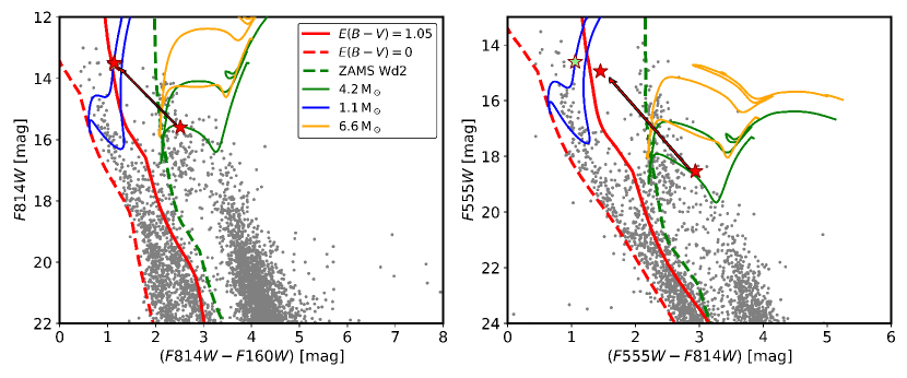
Figure 4: We show the $F814W-F160W$ vs. $F814W$ (left panel) and $F555W-F814W$ vs. $F555W$ (right panel) CMDs. The red (dashed) lines mark the field star sequences as defined in Hur et al. (2015).The green dashed line is the ZAMS for Wd2 (Zeidler et al., 2015). The green and yellow lines are the evolutionary tracks for the G5 ($4.25\,{\rm M}_{\odot}$) and B4.5 ($6.6\,{\rm M}_{\odot}$) cluster member stars, respectively. The red stars mark the loci of the star #10225 for the star being a cluster member and the star begin a foreground object. The blue line represents the evolutionary track of a $1.1\,{\rm M}_{\odot}$ star, the best-fitting solution if star #10225 is a field star. The green star marks the position of #10225 if we use an abnormal exinction law of $R_{\rm V}=2.45$ and $E(B-V)_{\rm fg}=1.55\,{\rm mag}$.

With the above argumentation in mind, we conclude that star #10225 is a cluster member with a spectral type of G5 PMS. Although possible, the offset between the evolutionary track and the star’s extinction corrected location in the $F555W-F814W$ vs. $F555W$ CMD on the one side and the well fitting locus as a cluster member on the other, makes it unlikely that the star is a foreground interloper.

5 The radial velocities

The stellar velocity dispersion of young star clusters is typically on the order of $\sim 5\,{\rm km}\,{\rm s}^{-1}$ (e.g., Rochau et al., 2010; Pang et al., 2013; Cottaar & Hénault-Brunet, 2014; Kiminki & Smith, 2018). To measure these velocities high-resolution spectrographs are typically used (with resolving power of $R\approx 30000$–60000). MUSE was designed to study high-redshift galaxy formation and star-formation in nearby galaxies, whose expected radial velocity (RV) dispersions are on the order of a few $100\,{\rm km}\,{\rm s}^{-1}$. To measure RVs of YMCs in the MW with MUSE we take advantage of the large wavelength range, allowing us to simultaneously measure RVs from a number of strong stellar absorption lines. Together with a statistical approach this allows us to reach the needed accuracy of a few ${\rm km}/{\rm s}$. The procedure is explained in the following section.

5.1 The stars

We selected a number of strong stellar absorption lines to measure the RVs: He II$\lambda 4685$, Mg I$\lambda\lambda 5267,5172,5183$, He II$\lambda 5411$, He I$\lambda 5876$, He II$\lambda 5411$, He I$\lambda 5876$, Fe II$\lambda 6456$, He I$\lambda 6678$, Ca II$\lambda\lambda 8498,4542,8662$. We intentionally did not use the H$\alpha$ and H$\beta$ lines because these lines may be contaminated by outflows and disks, especially for the young cluster stars.

To create a template for each of the lines, we used pyspeckit to fit Voigt-profiles (which is a convolution of a Gaussian and a Lorentzian profile) to the lines. The Voigt profile is defined as follows:

$$V\left(x,\sigma,\gamma\right)=\frac{\Re\left[w\left(z\right)\right]}{\sigma\sqrt{2\pi}},$$ (5)

where $\sigma$ is the width of the Gaussian and $\gamma$ the width of the Lorentzian. $\Re\left[w\left(z\right)\right]$ is the real part of the Faddeeva function evaluated for:

$$z=\frac{x+\i\gamma}{\sigma\sqrt{2}}.$$ (6)

Similar to what was done in Sect. 4 we used a $1^{\rm st}$ or $2^{\rm nd}$ order polynomial to model the continuum (depending on each line). We modeled all lines in each of the wavelength regions simultaneously. Using a Voigt profile and a small wavelength range resulted in optimized fits and line parameters. We then used the central wavelength extracted from the NIST library, while for the other parameters (amplitude, $\sigma$, and $\gamma$) we used the results from the above described line fitting. These templates, together with the observed spectra were fed into pPXF, which cross-correlates the template and the measured spectrum. Since our cluster-member stars are young stars possibly containing outflows, we only used the cores of each line. To make sure the determined velocities are not dominated by noise, we adopted a Monte-Carlo (MC) approach, where we repeated the cross correlation 20000 times. For each iteration the uncertainties where added, following a random normal distribution. The mean of the resulting Gaussian distribution was used as the measured RV and the width as its uncertainty. As a first step, we determined the RV of each line individually and applied a sigma clipping in velocity space. Using a $3\sigma$ threshold has proven to be sufficient to remove ”outliers” caused by peculiar line shapes (e.g., non-perfect background subtraction, remaining cosmic rays, or a non-perfect wavelength calibration). In a second step, we reprocessed the complete spectrum for a final velocity solution. Again, the mean of the resulting Gaussian distribution was used as the measured RV and the width as RV uncertainty. The radial velocities and their uncertainties are shown in Column 8 and 9 of Tab. 3. The typical RV uncertainty is $\sigma_{\rm RV}=2.90\,{\rm km}\,{\rm s}^{-1}$.

The limited spectral resolution of MUSE makes it necessary to carefully check whether the resulting RVs are reliable. While looking for binaries Rauw et al. (2011) measured RVs of different stellar lines for a small sample of stars in Wd2. Five of these stars have RV measurements that can be used as a comparison sample. Additionally, for three stars RV measurements are available in the Gaia data release 2 (DR2, Gaia Collaboration et al., 2016, 2018). The overall, error-weighted RV difference is $3.70\,{\rm km}\,{\rm s}^{-1}$. In Fig. 5 we show the Rauw et al. (2011) measurements (black) and Gaia measurements (red) vs. ours, confirming that reliable RVs with an accuracy of 2–$3\,{\rm km}\,{\rm s}^{-1}$ can be measured with MUSE when multiple stellar lines are used. The typical RV uncertainty of our measurements is $\sigma_{\rm RV}=2.90\,{\rm km}\,{\rm s}^{-1}$, which is similar to the results found in Kamann et al. (2016). Their median RV uncertainty is $3.0\,{\rm km}\,{\rm s}^{-1}$ for stars whose spectra have a S/N$>28$, which is comparable to our selected sample. Moreover, in their MUSE study of 500000 spectra of 200000 stars located in 22 globular clusters, Kamann et al. (2018) were able to reach a RV accuracy of $1\,{\rm km}\,{\rm s}^{-1}$ .

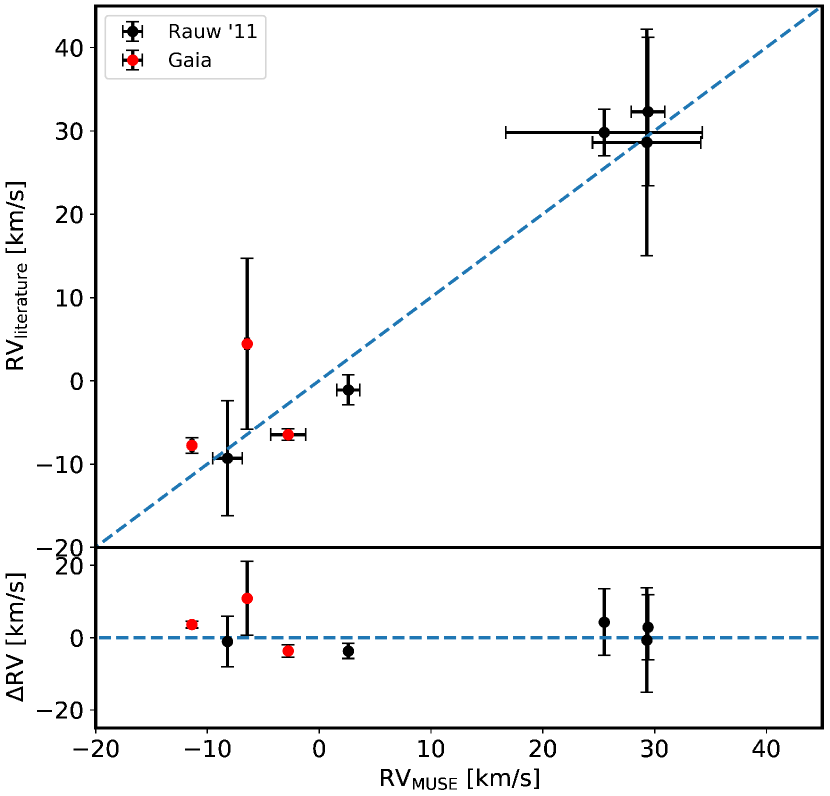
Figure 5: The RV comparison between our RV measurements (x-axis) and the existing literature values (y-axis, Rauw et al. (2011) measurements in black and Gaia measurements in red). The blue line is the theoretical 1:1 relation. The bottom plot shows the difference between our results and the literature values.

5.2 The gas

The same procedure can be used to measure the velocities of different gas emission lines. To increase the S/N, for the gas we always combined at least 3 spaxels as extracted from the reduced spectral cubes. We used three different sets of emission lines, the Balmer lines (${\rm H}\alpha$ and ${\rm H}\beta$), the [N II]$\lambda\lambda 6549,6583$ lines, and the [S II]$\lambda\lambda 6717,6731$ lines. We measured the gas velocities in regions not contaminated by bright stars.

6 Results and discussion

6.1 The spectral types – Cluster members vs. field stars

To avoid biases, we have so far treated all stars independently of whether they are cluster members or not. To study the internal dynamics of the NB as well as its origin, we need to distinguish between cluster member stars and field stars. Due to the young age of Wd2, we expect the early-type stars to belong to the cluster and not to the field, where the earliest types (O and B) have disappeared, due to their short lifetime (e.g., Massey, 2003). Since the most luminous stars in our data have a spectral ${\rm S/N}\geq 20$, we do not expect to see cluster members with a spectral type much later than an A-type star. The field stars may cover a by far wider dynamic range for their spectral types due to a much lower extinction compared to Wd2 ($A_{\rm V}=6.12\,{\rm mag}$, Zeidler et al., 2015). This high extinction is also the reason why we expect that all field stars detected in our MUSE spectra are located in front of Wd2.

We used our HST photometric catalog to create multiple CMDs (see Fig. 6) and marked all stars located in the NB, of which we determined their spectral type (red and black asterisks in Fig. 6). In Zeidler et al. (2015) we showed that the field stars and the cluster members can be well separated by a linear cut in color-magnitude space, represented by the blue line in Fig. 6. Comparing spectral types and locations in the CMDs, we see that the earliest spectral type among field stars is A9V, while OB stars appear to be cluster members except star #10255 (see Sect. 4.2.4 for a detailed discussion).

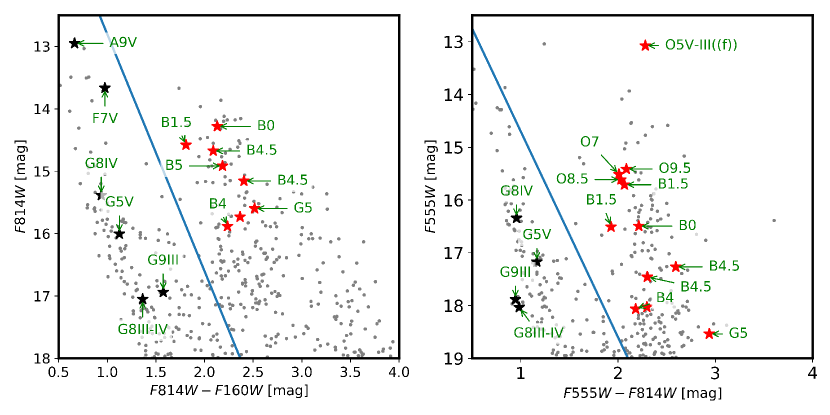
Figure 6: The $F814W-F160W$ vs. $F814W$ (left panel) and $F555W-F814W$ vs. $F555W$ (right panel) CMDs of all stars detected in our HST catalog (gray small dots). The blue line shows the photometrically estimated separation between the cluster members and field stars (Zeidler et al., 2015). The stars in the NB whose spectral type was derived from our MUSE data are marked with asterisks.

This analysis is based only on stars in the NB. It shows that, for a given magnitude range, the spectral types may be used as an additional indicator to separate cluster members from field stars, which is important at loci where the two populations (cluster and field) are not very well separated.

6.2 The radial velocity distribution of Wd2

6.2.1 The stars

For the NB, there are 24 stars suited to measure RVs. To increase the sample for further statistical analyses of the stellar velocity distribution, we added 48 stars from the remaining cluster area including stars located in some of the recently obtained long exposures. These stars were selected based on their good-quality extracted spectra. An overview over all stars used for this work is presented in Tab. 3.

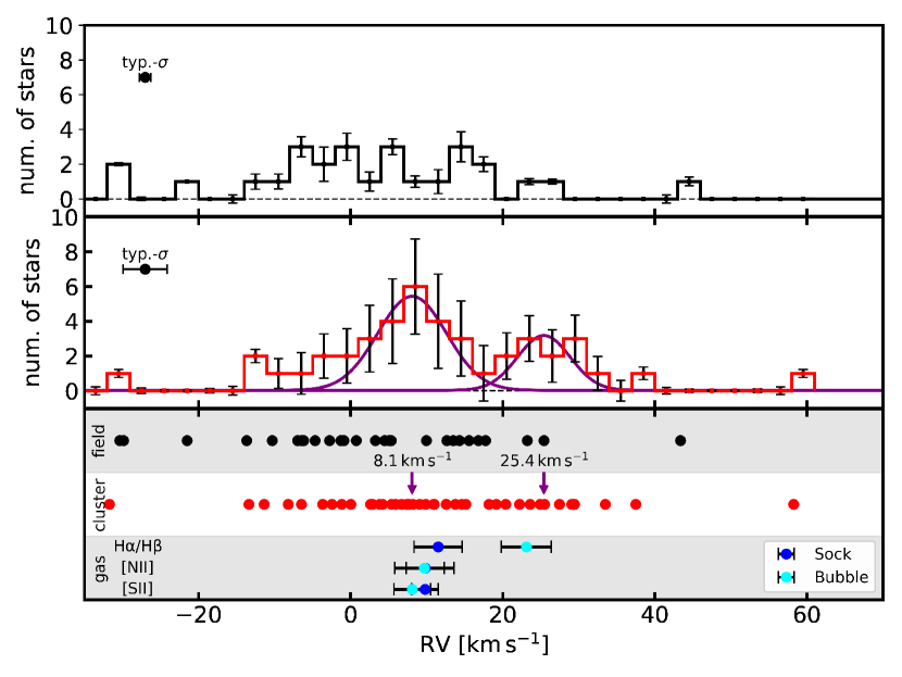
Figure 7: Top panel: The RV distribution of the field stars (black). We show the typical velocity uncertainty for a single star, obtained from the field stars only ($\sigma=0.76\,{\rm km}/{\rm s}$). Middle panel: The RV distribution of the cluster stars (red). We show the typical velocity uncertainty for a single star ($\sigma=2.90\,{\rm km}/{\rm s}$), as well as the number uncertainty per RV bin. The purple curves show the most probable result of the MCMC simulation for the bimodal distribution. Bottom panel: The locus of the cluster stars (red) and the field stars (black) in RV space. The mean RVs of $(8.10\pm 1.53)\,{\rm km}\,{\rm s}^{-1}$ and $(25.41\pm 1.57)\,{\rm km}\,{\rm s}^{-1}$ of the bimodal distribution are indicated by the purple arrows. We also show the median gas velocities measured from the Balmer lines ($(11.50\pm 3.15)\,{\rm km}\,{\rm s}^{-1}$ and $(23.09\pm 3.27)\,{\rm km}\,{\rm s}^{-1}$), the [N II]$\lambda\lambda 6549,6583$ lines ($(9.81\pm 2.50)\,{\rm km}\,{\rm s}^{-1}$ and $(9.70\pm 3.90)\,{\rm km}\,{\rm s}^{-1}$), and the [S II]$\lambda\lambda 6717,6731$ lines ($(9.77\pm 1.76)\,{\rm km}\,{\rm s}^{-1}$ and $(8.22\pm 2.42\,{\rm km}\,{\rm s}^{-1}$). The velocities are always given for ”the Sock” and the NB, respectively.

We analyzed the RV distribution throughout the Wd2 area including all 72 stars (see Tab. 3, faintest star: $V=20.53\,{\rm mag}$), 44 of which are cluster members, based on their location in the CMDs of Fig. 6. In the lower panel of Fig. 7 we show the RV distribution of the cluster members (red) and the field stars (black), where the binsize is set equal to the typical velocity uncertainty of $\sim 3\,{\rm km}/{\rm s}$. We propagated the individual measured RV uncertainty per star to a cumulative uncertainty on the number of stars per velocity bin, assuming they are Bernoulli distributed. As a result, also bins with no stars may have a non-zero uncertainty.

To quantify the distribution and to test whether it is statistically significant, we applied a Markov Chain Monte Carlo (MCMC) method on a combination of two Gaussian distributions and a common offset including the number uncertainties per RV bin. We ran $8\times 10^{5}$ random draws and confirmed the bimodal distribution. The most probable RV of each of the two peaks is $(8.10\pm 1.53)\,{\rm km}\,{\rm s}^{-1}$ and $(25.41\pm 1.57)\,{\rm km}\,{\rm s}^{-1}$. The $1\sigma$ widths of the two peaks are $(4.52\pm 1.78)\,{\rm km}\,{\rm s}^{-1}$ and $(3.46\pm 1.29)\,{\rm km}\,{\rm s}^{-1}$. To exclude a bias for the choice of the priors, we also ran the MCMC fit using a single Gaussian and a combination of three Gaussians, both with a common offset. Each MCMC run did not converge to a reliable solution.

We tested if the cluster and field populations are following different distributions. First, we tried to fit the same distribution as for the cluster members to the field population. This MCMC run did not converge to a reliable solution. Second, we ran a Kolmogorov-Smirnov (K.S.) test with the null hypothesis that the two populations are from the same parental sample. Based on the obtained p-value of 0.04, we can reject the null hypothesis. Both tests confirm that the field and the cluster population are indeed different.

To avoid being biased by the member selection performed with our HST catalog we used the Gaia DR2 as a third, independent test. Due to the high extinction and crowding toward Wd2 the parallaxes and proper motions of the majority of the stars in that region still have large uncertainties. We divided the stars in likely foreground field stars and likely cluster members based on the Gaia DR2 photometry (see left panel of Fig. 8). We then selected all probable cluster member stars, for which the proper motion uncertainty is less than $0.2\,{\rm mas\,yr}^{-1}$ (corresponding to $3.9\,{\rm km\,s}^{-1}$ in declination and $2.1\,{\rm km\,s}^{-1}$ in right ascension at a distance of 4.16 kpc, selecting 111 and 109 stars, respectively). We show the proper motions in right ascension and declination in the center and right panel of Fig. 8, respectively. The proper motion distribution in declination shows the same double peak as the RV distribution (see Fig. 7), supporting the bimodality of Wd2’s stellar population. In right ascension a double peak is not apparent. The reason for this may be a very small difference between the two peaks, not detectable by the current accuracy of the Gaia data. Another possibility is that due to the North - South orientation of the two clumps (Hur et al., 2015; Zeidler et al., 2015), such a bimodal distribution does not exist in this direction. Gaia DR3 will shade light on this. We cross matched the cluster stars for which we have RV measurements with the one for which we have proper motions. Their distribution is shown as green dashed histogram in Fig. 8. Both histograms show a bimodal distribution. The number of stars is not high enough to obtain a significant result from cross matching the two peaks individually. As in RV space, the velocity distribution of the field stars (bottom panels of Fig. 8) shows a uniform distribution with a similar velocity range as the cluster members. This excludes the possibility of using the proper motions for an additional criterion for the membership selection as it was done, e.g., the Orion Star Forming Complex (Kounkel et al., 2018).

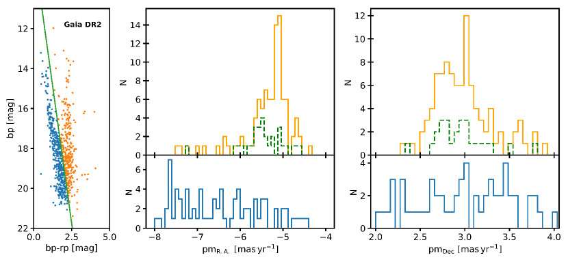
Figure 8: Left panel: The Gaia CMD toward Wd2. The green line separates likely cluster members (orange) from the likely field stars (blue). In total 421 field stars and 302 cluster members are detected. Center panel: The proper motion distribution in right ascension of all stars that have an uncertainty less than $0.2\,{\rm mas\,yr}^{-1}$. The top panel shows the cluster members while the bottom panel shows the field stars. Right panel: The proper motion distribution in declination of all stars that have an uncertainty less than $0.2\,{\rm mas\,yr}^{-1}$ showing a bimodal distribution. The top panel shows the cluster members while the bottom panel shows the field stars. The dashed green histograms show the distribution of the stars that also have MUSE RVs.

Comparing the velocity distribution of the RVs and in declination, in addition to the K.S. test, the MCMC fit, and the cross-matched histograms, we conclude that the Wd2 stars show a bimodal velocity distribution.

In Fig. 9 we show the location of all cluster members (left panel) and all field stars (right panel) color-coded by their respective RVs. The red square marks the $64^{\prime\prime}\times 64^{\prime\prime}$ region around the NB similar to Fig. 1. The selection of stars is fairly uniform. There is no hint of a spatial correlation, especially in the field stars. This shows that there are no calibration artifacts left, which may influence the accuracy of our results.

Figure 9: Left: The cluster-member stars in the NB for which we measured the RVs. The colorbar shows the measured RVs. To see more details we used the HST $F658N$ (${\rm H}\alpha$) image as background. Right: The field stars for which we measured the RVs.

Based on CO($J=1$–2) NANTEN2 sub-millimeter observations of RCW49, Furukawa et al. (2009) argued for the formation of Wd2 having been triggered by a collision between two molecular clouds ($\sim 4\,$Myr ago) as a viable scenario. The CO velocity profile of the whole region revealed that there are two gas clouds moving with an RV of $0^{+9}_{-11}\,{\rm km}\,{\rm s}^{-1}$, located in front of Wd2, and $16^{+5}_{-4}\,{\rm km}\,{\rm s}^{-1}$, respectively, located in the background of Wd2. The velocity difference of the two stellar components ($\Delta v_{\star}=(17.30\pm 2.17)\,{\rm km}\,{\rm s}^{-1}$) and the velocity difference of the two gas clouds ($\Delta v_{\rm gas}=16^{+10.3}_{-11.7}\,{\rm km}\,{\rm s}^{-1}$) are similar. Although the mean velocities of both clouds are lower than the velocities of the two stellar components they might be connected. A detailed RV analysis of all stars and the gas is necessary to establish a connection between the stellar RV distribution and a probable formation scenario of Wd2. We will address this in a future work analyzing the complete dataset.

In a recent study, Kiminki & Smith (2018) measured a velocity dispersion of $\leq 9.1\,{\rm km}\,{\rm s}^{-1}$ or 41 well-constrained O-type stars in the Trumpler 14 cluster in the Carina Nebula (e.g., Smith & Brooks, 2008, and references therein). Rochau et al. (2010) used HST/WFPC2 (Gonzaga & Biretta, 2010) observations to measure proper motions of NGC 3603 and determined a 1D velocity dispersion of $(4.5\pm 0.8)\,{\rm km}\,{\rm s}^{-1}$. Pang et al. (2013) repeated the analysis with the same dataset but for each tangential component individually resulting in an slightly increased velocity dispersion ($\sigma_{x}=(4.8\pm 0.5)\,{\rm km}\,{\rm s}^{-1}$ and $\sigma_{y}=(6.5\pm 0.5)\,{\rm km}\,{\rm s}^{-1}$), which was most likely caused by a different selection method and detection uncertainty correction. Comparing these studies to the $1\sigma$ widths of the two RV distributions in Wd2 ($(4.52\pm 1.78)\,{\rm km}\,{\rm s}^{-1}$ and $(3.46\pm 1.29)\,{\rm km}\,{\rm s}^{-1}$) we can conclude that the RV dispersions derived for the two components of Wd2 are comparable with measurements for other Galactic YMCs. We will perform a detailed velocity dispersion analysis and estimates of the dynamical cluster mass in a future paper.

6.2.2 The gas

To study the velocity distribution of the gas we chose 20 fields across the NB with a typical size of $1.715\times 1.715\,{\rm arcsec}^{2}$ or $8.575\times 8.575\,{\rm px}^{2}$ (see Fig. 10). For ”the Sock” we used 102 smaller, elliptically-shaped fields to cover the rims on both sides, as well as visible features of the gas (e.g., a possible bow shock). The typical size of an ellipse is $0.12\,{\rm arcsec}^{2}$, which corresponds to $\sim 3\,$px². All of the covered areas where chosen in a way that excludes stars. In Fig. 10 and Fig. 11 we present the results for the distributions in gas velocity for the NB and the rims of ”the Sock”, respectively.

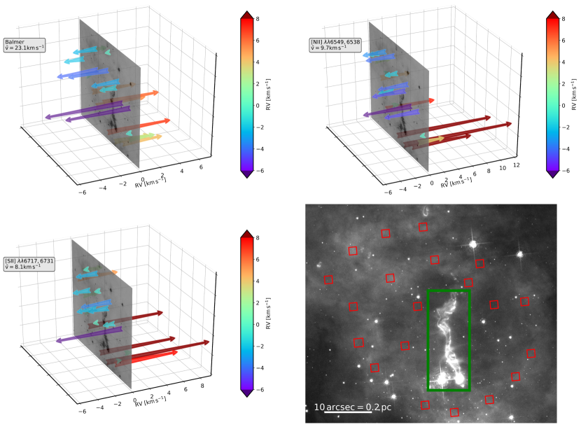
Figure 10: The gas velocities of the NB derived from the Balmer lines, the [N II]$\lambda\lambda 6549,6583$ lines, and the [S II]$\lambda\lambda 6717,6731$ lines. We use the respective median velocity (indicated in the top left corner) as reference frame. The arrows represent the line-of-sight velocities. We chose the HST $F658N$ (${\rm H}\alpha$) filter as reference image. The typical velocity uncertainty is $0.7\,{\rm km}\,{\rm s}^{-1}$, derived in the same manner as the stellar RVs and their uncertainties. In the bottom right panel we show the H$\alpha$ image face-on and marked the 20 fields where we measured the RVs with red squares. The green area marks ”the Sock” (see Fig. 11). North is up, East is to the left.

The median velocity of each element of the NB and ”the Sock” is reported in the bottom panel of Fig. 7. The median gas velocities are, within the uncertainties in agreement with the stellar velocities of the blue shifted peak, thus evidencing a spatial connection between gas and stars, with the latter being formed in the cavity of the gas cloud. The median gas velocity of the NB as derived from the Balmer lines appears to be $\sim 11\,{\rm km}\,{\rm s}^{-1}$ higher than all the other RV measurements, indicating a more complicated velocity structure. The whole NB appears to be slightly red-shifted, indicating that it is moving away from us.

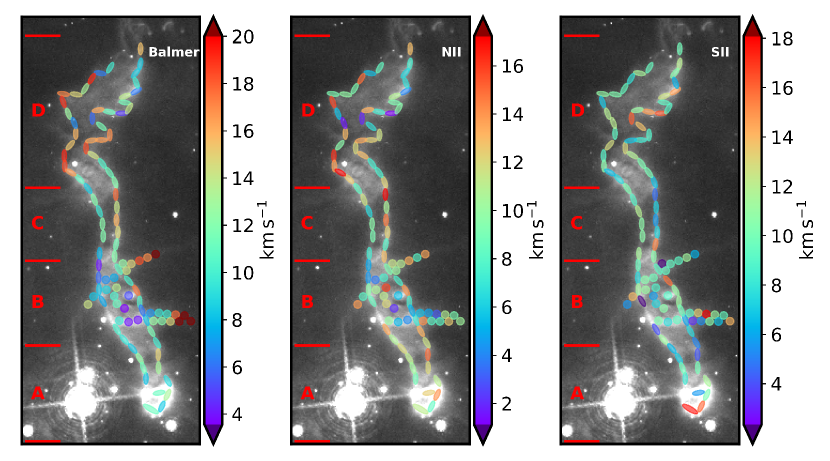
Figure 11: The gas velocities of ”the Sock” (marked in green in Fig. 10) derived from the Balmer lines, the [N II]$\lambda\lambda 6549,6583$ lines, and the [S II]$\lambda\lambda 6717,6731$ lines. We use the respective median velocity (indicated in the top left corner) as reference frame. The four main regions are marked on the left. To see more details we selected the HST $F658N$ (${\rm H}\alpha$) image as background. The typical velocity uncertainty is $0.4\,{\rm km}\,{\rm s}^{-1}$, derived in the same manner than the stellar RVs. The luminous star to the South-East has a spectral type of O5III-V((f)) (Vargas Álvarez et al., 2013). Each panel shows $9"\times 22"$. North is up, East is to the left.

To better compare the velocities of the various components, we subtracted the median velocity for each of the three elements in Fig. 10 and Fig. 11. The median velocity of the gas is also presented in the bottom panel of Fig. 7. The RVs of the gas in the NB indicate rotation probably caused by the winds from the massive O-stars inside the NB. The South-East side moves away from us while the North-West side moves toward us (see Fig. 10). We divided ”the Sock” in four major regions labeled A to D as we move from South to North (see Fig. 11). Looking at the gas RVs of ”the Sock”, derived by analyzing the Balmer lines, it shows a ”twisted” velocity profile:

• The stars located East of the tip show similar velocities as ”the Sock”, which is a strong indication that they are spatially connected. We suggest that the slightly arch-shaped morphology of ”the Sock” is caused by the O5III-V((f)) star. Due to insufficient S/N we were unable to extract useful spectra for the two sources directly located at the tip. The left and the right rims have similar velocities.

• There appears to be a bow-shock pointing South-East with a star embedded in the gas or located behind ”the Sock” and therefore not visible. The hydrogen lines of the tail of the bow-shock are more red-shifted than the tip of the bow-shock, which cannot be detected in [S II] and [N II].

• The right rim appears to be red-shifted compared to the left side which suggests rotation or expansion. This profile is reversed when looking at the [S II] lines

• The northern end shows a chaotic structure both in velocity space and in real space, which might be caused by some external disturbance or by the interaction of ”the Sock” with the edge on the NB.

Overall, the RV profile of ”the Sock”, derived using the Balmer and [N II] lines, appears to be twisted with a chaotic northern end. The RV distribution appears more uniform using the [S II] lines, indicating a complex velocity profile that needs to be further investigated. Deriving gas abundance and temperatures including the influence of all the surrounding stellar sources not only of the NB but of the whole Wd2 region is left for a future paper once the full dataset including the long exposures is fully reduced and analyzed.

7 Summary and conclusions

In this work we have presented the first results of the combined study of VLT/MUSE integral field spectroscopy and high-resolution HST photometry of the young massive cluster Wd2 with the aim of studying its stellar and gaseous components in great detail. We focused on a field North of the main cluster, which we call the Northern Bubble, a cavity blown into the remaining gas of the parental gas cloud. In its center, a pillar-like structure or jet-like object, ”the Sock”, is present (see Fig. 2).

We extracted spectra for 17 stars located in the NB, which are suitable for a spectral classification, using the python based code PampelMuse (Kamann et al., 2013). Depending on the spectral type, we cross-matched libraries of the Ca II-triplet region with the observed spectra (stellar type: A9 and later) or used EW ratios of helium and hydrogen lines (O and B stars). These methods give comparable results to the more traditional way of by-eye comparison with template spectra. With this method the majority of stars can be automatically classified, which will become important as soon as we have the complete dataset of $\gtrapprox 1000$ spectra.

We added another 2 O and 5 B-type stars to the 37 already known OB-type stars (Moffat et al., 1991; Vargas Álvarez et al., 2013) in Wd2.

Using strong stellar absorption lines, we derived stellar RVs of 72 stars throughout the Wd2 cluster area with an accuracy of $2.9\,{\rm km\,s}^{-1}$ . The cluster member stars follow a bimodal velocity distribution centered on $(8.10\pm 1.53)\,{\rm km}\,{\rm s}^{-1}$ and $(25.41\pm 1.57)\,{\rm km}\,{\rm s}^{-1}$ (see Fig. 7) with a dispersion of $(4.52\pm 1.78)\,{\rm km}\,{\rm s}^{-1}$ and $(3.46\pm 1.29)\,{\rm km}\,{\rm s}^{-1}$, respectively. The dispersions are comparable to those of other Galactic YMCs, such as NGC 3603 (Rochau et al., 2010; Pang et al., 2013) or Trumpler 14 in the Carina Nebula (Kiminki & Smith, 2018). The bimodal distribution is also seen in the proper motions of the Gaia DR2 photometric catalog.

These first results show that it is indeed possible to extract stellar spectra in YMCs from MUSE data to an accuracy where it is possible to estimate the velocity dispersion of PMS stars. We also showed that we can analyze the gas and stars and confirm whether the different components are actually spatially connected.

Appendix A The properties of the stars used in this work

In Tab. 3 we present all stars and their properties used in the analyses of this paper.

Table 3: The analyzed stars

ID	R.A.	Dec.	$F555W$	$F814W$	$F160W$	$F814W_{\rm spec}$	rv	$\sigma_{\rm rv}$	${\rm N}_{\rm lines}$	spectral type
	(J2000)		[mag]				[km/s]
Northern Bubble stars
6660	$10^{\mathrm{h}}24^{\mathrm{m}}00.46^{\mathrm{s}}$	$-57^{\circ}44{}^{\prime}37.43{}^{\prime\prime}$	17.459	15.157	12.751	14.952	-1.168	3.273	3	B4.5
6687	$10^{\mathrm{h}}24^{\mathrm{m}}00.49^{\mathrm{s}}$	$-57^{\circ}44{}^{\prime}44.45{}^{\prime\prime}$	15.711	13.644	—	13.409	29.302	4.852	1	B1.5
7057	$10^{\mathrm{h}}24^{\mathrm{m}}00.85^{\mathrm{s}}$	$-57^{\circ}44{}^{\prime}27.17{}^{\prime\prime}$	18.065	15.883	13.646	15.634	24.906	2.029	3	B4
7510	$10^{\mathrm{h}}24^{\mathrm{m}}01.26^{\mathrm{s}}$	$-57^{\circ}44{}^{\prime}23.01{}^{\prime\prime}$	16.496	14.282	12.150	14.026	15.132	1.713	2	B0
8586	$10^{\mathrm{h}}24^{\mathrm{m}}02.22^{\mathrm{s}}$	$-57^{\circ}44{}^{\prime}35.48{}^{\prime\prime}$	18.030	15.733	13.367	15.318	-2.446	4.840	2	—
8768	$10^{\mathrm{h}}24^{\mathrm{m}}02.39^{\mathrm{s}}$	$-57^{\circ}44{}^{\prime}34.80{}^{\prime\prime}$	15.512	13.502	—	13.163	9.851	2.571	2	O7.5
8806	$10^{\mathrm{h}}24^{\mathrm{m}}02.43^{\mathrm{s}}$	$-57^{\circ}44{}^{\prime}36.09{}^{\prime\prime}$	13.076	—	—	10.794	2.611	1.038	2	O5V-III((f))
9186	$10^{\mathrm{h}}24^{\mathrm{m}}02.78^{\mathrm{s}}$	$-57^{\circ}44{}^{\prime}37.64{}^{\prime\prime}$	16.508	14.579	12.769	14.365	8.184	1.138	2	B1.5
9529	$10^{\mathrm{h}}24^{\mathrm{m}}03.09^{\mathrm{s}}$	$-57^{\circ}44{}^{\prime}17.48{}^{\prime\prime}$	—	14.480	12.730	14.480	58.227	2.959	3	B5
10198	$10^{\mathrm{h}}24^{\mathrm{m}}03.77^{\mathrm{s}}$	$-57^{\circ}44{}^{\prime}39.79{}^{\prime\prime}$	15.414	13.328	—	13.091	29.056	1.156	4	O9.5
10225	$10^{\mathrm{h}}24^{\mathrm{m}}03.80^{\mathrm{s}}$	$-57^{\circ}44{}^{\prime}34.92{}^{\prime\prime}$	18.539	15.600	13.084	15.154	7.745	1.112	2	G5
10372	$10^{\mathrm{h}}24^{\mathrm{m}}03.97^{\mathrm{s}}$	$-57^{\circ}44{}^{\prime}36.59{}^{\prime\prime}$	15.615	13.585	—	13.399	27.453	3.622	3	O8.5
10759	$10^{\mathrm{h}}24^{\mathrm{m}}04.40^{\mathrm{s}}$	$-57^{\circ}44{}^{\prime}36.17{}^{\prime\prime}$	17.268	14.674	12.584	14.375	22.216	2.598	2	B4.5
11126	$10^{\mathrm{h}}24^{\mathrm{m}}04.83^{\mathrm{s}}$	$-57^{\circ}44{}^{\prime}11.42{}^{\prime\prime}$	19.446	17.167	14.984	—	2.857	1.927	2	—
11414	$10^{\mathrm{h}}24^{\mathrm{m}}05.17^{\mathrm{s}}$	$-57^{\circ}44{}^{\prime}36.65{}^{\prime\prime}$	19.148	16.380	13.733	—	0.025	3.829	2	—
12258	$10^{\mathrm{h}}24^{\mathrm{m}}06.21^{\mathrm{s}}$	$-57^{\circ}44{}^{\prime}42.96{}^{\prime\prime}$	17.943	15.439	12.663	—	-48.172	9.338	2	—
cluster members in the remaining Wd2 cluster
2651	$10^{\mathrm{h}}23^{\mathrm{m}}55.16^{\mathrm{s}}$	$-57^{\circ}45{}^{\prime}26.88{}^{\prime\prime}$	—	—	—	—	25.505	8.789	2	—
3077	$10^{\mathrm{h}}23^{\mathrm{m}}55.88^{\mathrm{s}}$	$-57^{\circ}44{}^{\prime}24.01{}^{\prime\prime}$	18.441	16.007	—	—	6.693	6.642	2	—
3904	$10^{\mathrm{h}}23^{\mathrm{m}}57.23^{\mathrm{s}}$	$-57^{\circ}44{}^{\prime}37.91{}^{\prime\prime}$	16.358	13.918	—	—	10.984	3.224	4	—
3934	$10^{\mathrm{h}}23^{\mathrm{m}}57.26^{\mathrm{s}}$	$-57^{\circ}44{}^{\prime}06.98{}^{\prime\prime}$	—	25.212	19.112	—	14.614	4.919	2	—
4221	$10^{\mathrm{h}}23^{\mathrm{m}}57.68^{\mathrm{s}}$	$-57^{\circ}45{}^{\prime}26.68{}^{\prime\prime}$	20.528	17.089	13.612	—	-31.711	3.995	3	—
4246	$10^{\mathrm{h}}23^{\mathrm{m}}57.71^{\mathrm{s}}$	$-57^{\circ}45{}^{\prime}34.24{}^{\prime\prime}$	16.959	14.649	12.387	—	20.387	4.927	2	—
4821	$10^{\mathrm{h}}23^{\mathrm{m}}58.43^{\mathrm{s}}$	$-57^{\circ}45{}^{\prime}12.95{}^{\prime\prime}$	16.287	13.770	—	—	12.586	2.737	4	—
4948	$10^{\mathrm{h}}23^{\mathrm{m}}58.58^{\mathrm{s}}$	$-57^{\circ}45{}^{\prime}05.40{}^{\prime\prime}$	19.370	16.829	13.298	—	5.376	10.178	1	—
5476	$10^{\mathrm{h}}23^{\mathrm{m}}59.24^{\mathrm{s}}$	$-57^{\circ}45{}^{\prime}39.73{}^{\prime\prime}$	18.403	15.926	13.509	15.593	23.599	5.311	2	—
5505	$10^{\mathrm{h}}23^{\mathrm{m}}59.26^{\mathrm{s}}$	$-57^{\circ}45{}^{\prime}05.67{}^{\prime\prime}$	19.043	16.462	13.746	—	-3.682	2.850	2	—
5773	$10^{\mathrm{h}}23^{\mathrm{m}}59.54^{\mathrm{s}}$	$-57^{\circ}45{}^{\prime}22.49{}^{\prime\prime}$	13.042	11.800	—	11.534	18.179	0.168	2	—
5870	$10^{\mathrm{h}}23^{\mathrm{m}}59.66^{\mathrm{s}}$	$-57^{\circ}45{}^{\prime}06.48{}^{\prime\prime}$	17.368	15.182	13.096	14.903	10.906	2.301	2	—
6019	$10^{\mathrm{h}}23^{\mathrm{m}}59.82^{\mathrm{s}}$	$-57^{\circ}45{}^{\prime}15.58{}^{\prime\prime}$	17.863	15.680	13.601	15.437	7.387	3.984	2	—
6342	$10^{\mathrm{h}}24^{\mathrm{m}}00.14^{\mathrm{s}}$	$-57^{\circ}45{}^{\prime}29.76{}^{\prime\prime}$	18.145	15.519	12.962	15.277	3.832	4.970	2	—
6391	$10^{\mathrm{h}}24^{\mathrm{m}}00.18^{\mathrm{s}}$	$-57^{\circ}45{}^{\prime}32.53{}^{\prime\prime}$	16.102	13.861	11.692	13.570	12.539	1.961	4	—
6528	$10^{\mathrm{h}}24^{\mathrm{m}}00.34^{\mathrm{s}}$	$-57^{\circ}45{}^{\prime}42.62{}^{\prime\prime}$	15.880	13.510	—	13.171	37.477	5.312	1	—
7620	$10^{\mathrm{h}}24^{\mathrm{m}}01.38^{\mathrm{s}}$	$-57^{\circ}45{}^{\prime}29.58{}^{\prime\prime}$	14.085	12.045	—	11.705	4.209	2.534	2	—
8174	$10^{\mathrm{h}}24^{\mathrm{m}}01.85^{\mathrm{s}}$	$-57^{\circ}45{}^{\prime}31.17{}^{\prime\prime}$	15.917	13.758	—	13.576	9.065	2.807	2	—
8728	$10^{\mathrm{h}}24^{\mathrm{m}}02.35^{\mathrm{s}}$	$-57^{\circ}45{}^{\prime}30.56{}^{\prime\prime}$	13.942	—	—	11.181	29.419	1.512	1	—
9013	$10^{\mathrm{h}}24^{\mathrm{m}}02.62^{\mathrm{s}}$	$-57^{\circ}45{}^{\prime}37.43{}^{\prime\prime}$	16.143	13.965	12.007	13.791	-13.374	3.378	2	—
10048	$10^{\mathrm{h}}24^{\mathrm{m}}03.59^{\mathrm{s}}$	$-57^{\circ}45{}^{\prime}27.08{}^{\prime\prime}$	16.809	14.551	12.461	14.285	7.546	3.194	2	—
11178	$10^{\mathrm{h}}24^{\mathrm{m}}04.89^{\mathrm{s}}$	$-57^{\circ}45{}^{\prime}28.35{}^{\prime\prime}$	14.607	12.254	—	11.963	-8.204	1.326	3	—
12154	$10^{\mathrm{h}}24^{\mathrm{m}}06.09^{\mathrm{s}}$	$-57^{\circ}45{}^{\prime}57.65{}^{\prime\prime}$	18.008	15.342	12.913	15.567	33.474	3.056	2	—
13585	$10^{\mathrm{h}}24^{\mathrm{m}}07.91^{\mathrm{s}}$	$-57^{\circ}44{}^{\prime}23.46{}^{\prime\prime}$	17.395	15.451	13.702	—	5.915	11.727	1	—
14138	$10^{\mathrm{h}}24^{\mathrm{m}}08.68^{\mathrm{s}}$	$-57^{\circ}46{}^{\prime}02.42{}^{\prime\prime}$	18.165	15.828	13.380	16.076	13.768	2.527	2	—
14161	$10^{\mathrm{h}}24^{\mathrm{m}}08.74^{\mathrm{s}}$	$-57^{\circ}44{}^{\prime}43.97{}^{\prime\prime}$	19.653	17.121	14.563	—	-6.481	2.515	5	—
14213	$10^{\mathrm{h}}24^{\mathrm{m}}08.82^{\mathrm{s}}$	$-57^{\circ}44{}^{\prime}36.56{}^{\prime\prime}$	16.666	14.834	—	—	19.159	0.717	5	—
15613	$10^{\mathrm{h}}24^{\mathrm{m}}10.69^{\mathrm{s}}$	$-57^{\circ}46{}^{\prime}00.00{}^{\prime\prime}$	16.387	12.783	—	12.983	-11.379	0.171	3	—
Field stars in the Northern Bubble
6446	$10^{\mathrm{h}}24^{\mathrm{m}}00.25^{\mathrm{s}}$	$-57^{\circ}44{}^{\prime}07.96{}^{\prime\prime}$	—	—	12.690	13.230	4.480	0.212	6	F7V
6542	$10^{\mathrm{h}}24^{\mathrm{m}}00.35^{\mathrm{s}}$	$-57^{\circ}44{}^{\prime}17.50{}^{\prime\prime}$	18.035	17.051	15.686	16.655	16.792	1.254	4	G8III-IV
6717	$10^{\mathrm{h}}24^{\mathrm{m}}00.51^{\mathrm{s}}$	$-57^{\circ}44{}^{\prime}26.49{}^{\prime\prime}$	17.171	16.005	14.879	15.843	-0.896	1.212	2	G5V
7830	$10^{\mathrm{h}}24^{\mathrm{m}}01.55^{\mathrm{s}}$	$-57^{\circ}44{}^{\prime}05.68{}^{\prime\prime}$	—	—	12.285	12.514	17.746	0.353	3	A9V
10615	$10^{\mathrm{h}}24^{\mathrm{m}}04.26^{\mathrm{s}}$	$-57^{\circ}44{}^{\prime}22.92{}^{\prime\prime}$	16.344	15.387	14.448	15.216	15.557	0.448	4	G8IV var
10733	$10^{\mathrm{h}}24^{\mathrm{m}}04.37^{\mathrm{s}}$	$-57^{\circ}44{}^{\prime}28.51{}^{\prime\prime}$	17.884	16.938	15.362	16.390	43.358	1.496	2	G9III
11065	$10^{\mathrm{h}}24^{\mathrm{m}}04.75^{\mathrm{s}}$	$-57^{\circ}44{}^{\prime}32.95{}^{\prime\prime}$	16.469	15.587	14.718	15.409	3.263	0.610	4	—
11549	$10^{\mathrm{h}}24^{\mathrm{m}}05.32^{\mathrm{s}}$	$-57^{\circ}44{}^{\prime}44.24{}^{\prime\prime}$	19.082	17.037	15.093	—	9.966	2.315	3	—
Field stars in the remaining Wd2 cluster
5753	$10^{\mathrm{h}}23^{\mathrm{m}}59.52^{\mathrm{s}}$	$-57^{\circ}46{}^{\prime}42.55{}^{\prime\prime}$	15.893	15.036	14.232	14.940	-30.347	0.476	5	—
6973	$10^{\mathrm{h}}24^{\mathrm{m}}00.75^{\mathrm{s}}$	$-57^{\circ}46{}^{\prime}29.58{}^{\prime\prime}$	14.291	13.506	12.721	13.397	14.301	0.268	5	—
7109	$10^{\mathrm{h}}24^{\mathrm{m}}00.90^{\mathrm{s}}$	$-57^{\circ}46{}^{\prime}10.69{}^{\prime\prime}$	16.553	15.621	14.684	15.503	13.477	1.807	2	—
7282	$10^{\mathrm{h}}24^{\mathrm{m}}01.06^{\mathrm{s}}$	$-57^{\circ}46{}^{\prime}18.63{}^{\prime\prime}$	15.735	14.808	13.899	14.717	-21.500	0.491	2	—
8584	$10^{\mathrm{h}}24^{\mathrm{m}}02.21^{\mathrm{s}}$	$-57^{\circ}45{}^{\prime}02.65{}^{\prime\prime}$	13.869	13.032	12.271	12.837	-6.442	0.209	6	—
9577	$10^{\mathrm{h}}24^{\mathrm{m}}03.14^{\mathrm{s}}$	$-57^{\circ}45{}^{\prime}21.12{}^{\prime\prime}$	17.017	15.890	14.776	15.645	-43.813	0.796	4	—
9709	$10^{\mathrm{h}}24^{\mathrm{m}}03.26^{\mathrm{s}}$	$-57^{\circ}45{}^{\prime}50.83{}^{\prime\prime}$	17.389	16.356	15.334	16.221	-29.858	0.695	5	—
9849	$10^{\mathrm{h}}24^{\mathrm{m}}03.40^{\mathrm{s}}$	$-57^{\circ}46{}^{\prime}09.64{}^{\prime\prime}$	15.065	14.308	13.600	14.214	25.433	0.455	3	—
11134	$10^{\mathrm{h}}24^{\mathrm{m}}04.84^{\mathrm{s}}$	$-57^{\circ}45{}^{\prime}49.88{}^{\prime\prime}$	16.970	15.799	14.653	15.648	12.653	0.707	5	—
12265	$10^{\mathrm{h}}24^{\mathrm{m}}06.21^{\mathrm{s}}$	$-57^{\circ}46{}^{\prime}10.31{}^{\prime\prime}$	16.048	15.198	14.475	15.500	23.228	0.629	5	—
12428	$10^{\mathrm{h}}24^{\mathrm{m}}06.43^{\mathrm{s}}$	$-57^{\circ}44{}^{\prime}50.85{}^{\prime\prime}$	16.860	15.850	14.862	15.680	5.333	1.051	6	—
12826	$10^{\mathrm{h}}24^{\mathrm{m}}06.89^{\mathrm{s}}$	$-57^{\circ}46{}^{\prime}27.31{}^{\prime\prime}$	16.404	15.400	14.481	15.708	5.067	0.639	5	—
12987	$10^{\mathrm{h}}24^{\mathrm{m}}07.10^{\mathrm{s}}$	$-57^{\circ}46{}^{\prime}16.62{}^{\prime\prime}$	15.841	14.921	14.050	15.243	-4.665	0.756	3	—
13727	$10^{\mathrm{h}}24^{\mathrm{m}}08.10^{\mathrm{s}}$	$-57^{\circ}45{}^{\prime}40.33{}^{\prime\prime}$	15.778	14.939	14.115	15.101	-10.300	1.037	3	—
13850	$10^{\mathrm{h}}24^{\mathrm{m}}08.28^{\mathrm{s}}$	$-57^{\circ}44{}^{\prime}28.22{}^{\prime\prime}$	17.377	16.354	15.439	—	-6.961	1.277	3	—
13986	$10^{\mathrm{h}}24^{\mathrm{m}}08.47^{\mathrm{s}}$	$-57^{\circ}44{}^{\prime}28.84{}^{\prime\prime}$	16.390	15.537	14.739	15.542	-13.665	1.817	2	—
14186	$10^{\mathrm{h}}24^{\mathrm{m}}08.78^{\mathrm{s}}$	$-57^{\circ}44{}^{\prime}47.70{}^{\prime\prime}$	17.598	15.938	14.405	—	0.731	2.466	3	—
16080	$10^{\mathrm{h}}24^{\mathrm{m}}11.38^{\mathrm{s}}$	$-57^{\circ}45{}^{\prime}52.16{}^{\prime\prime}$	16.788	15.820	14.923	16.006	-1.286	0.795	2	—
17656	$10^{\mathrm{h}}24^{\mathrm{m}}14.19^{\mathrm{s}}$	$-57^{\circ}44{}^{\prime}44.92{}^{\prime\prime}$	14.734	14.038	13.425	14.099	-6.172	0.760	4	—
19296	$10^{\mathrm{h}}24^{\mathrm{m}}18.27^{\mathrm{s}}$	$-57^{\circ}45{}^{\prime}26.47{}^{\prime\prime}$	—	—	—	—	-2.767	1.572	2	—

Note. — In this table we summarize the properties of the 72 stars used in this work. Column 1 shows the identifier of our HST photometric catalog. Columns 2 & 3 give the stellar coordinates. Columns 4–6 show the HST photometry used in this analysis. Column 7 represents the $F814W$ magnitude based on the extracted spectrum. Columns 8 & 9 show the measured RVs of the stars including their uncertainty. Column 11 gives the number of lines used to measure the RV. Column 11 shows the spectral type derived in Sect. 4.2. Spectral types written in italics were recovered from the literature.

Appendix B The individual spectral classification

#6446: The bluest Pa line visible is Pa19 and the missing Si II$\lambda\lambda 6347,6371$ exclude the star from being a supergiant. These criteria and the best fitted Ca II-triplet suggest the star being a F7V star.

#6717: This star shows a weak Paschen series in comparison to the very pronounced Ca II-triplet. The last visible Paschen line is Pa17, which indicates a luminosity class V and a spectral type of late A, F, or G-type. A large number of ionized and neutral metals are visible (e.g., Mg I-triplet, S II, and many iron lines). The visibility of a weak Ti I$\lambda 8435$ line, which appears to be equally strong to the Fe I$\lambda 8468$ line, favors a spectral type later than early G. The best fitting template for Ca II-triplet is a G5V star which is in agreement with the above argumentation. Vargas Álvarez et al. (2013) argue for a spectral type of late O to early B based on weak He I lines. The existence of the Ca II-triplet rules out an OB-star. This discrepancy was probably caused by a low S/N of the spectrum used in the analysis by Vargas Álvarez et al. (2013).

#7830: This star has broad Balmer lines and strong Pa-lines with the presence of the Ca II-triplet, although the Pa lines are clearly dominating. In combination with a very strong O I-triplet ($\lambda\lambda 7772,7774,7775$) this appears to be a late A-type star. The last visible Pa line is Pa18 suggesting a luminosity class of II, IV, or V. The fact that it still shows the Ca II-triplet allows to use the spectral library (Cenarro et al., 2001) for classification, leading to a spectral type of A9V in agreement with the above argumentation.

#10615 and #6542: The appearance of ionized metals (e.g., C III$\lambda 4647$), an almost absent Pa-series, narrow Balmer lines, and the appearance of Ti I$\lambda 8435$ suggest a late G to early K-type star. The best-fitting model for #10615 is a G8IV star while for #6542 it is a G8III-IV star.

#10733: Showing narrow Balmer lines suggest a spectral type later than A0. The presence of many neutral metals, the lack of the O I$\lambda 7774$ line, and the almost absent Pa-series suggests a spectral type later than F5. The existence of the Ti I$\lambda 8435$ line together with neutral iron in the Ca II-triplet favors a later G type to early K type star. The best fitting template is a G9III star.

References

- Avila (2017) Avila, R. J. 2017, Advanced Camera for Surveys Instrument Handbook for Cycle 25 v. 16.0
- Bacon et al. (2010) Bacon, R., Accardo, M., Adjali, L., et al. 2010, in Proc. SPIE, Vol. 7735, Ground-based and Airborne Instrumentation for Astronomy III, 773508
- Banerjee & Kroupa (2015) Banerjee, S., & Kroupa, P. 2015, MNRAS, 447, 728
- Cappellari (2017) Cappellari, M. 2017, MNRAS, 466, 798
- Cappellari & Emsellem (2004) Cappellari, M., & Emsellem, E. 2004, PASP, 116, 138
- Cenarro et al. (2001) Cenarro, A. J., Cardiel, N., Gorgas, J., et al. 2001, MNRAS, 326, 959
- Choi et al. (2016) Choi, J., Dotter, A., Conroy, C., et al. 2016, ApJ, 823, 102
- Cignoni et al. (2009) Cignoni, M., Sabbi, E., Nota, A., et al. 2009, AJ, 137, 3668
- Cottaar & Hénault-Brunet (2014) Cottaar, M., & Hénault-Brunet, V. 2014, A&A, 562, A20
- Dotter (2016) Dotter, A. 2016, ApJS, 222, 8
- Dressel (2018) Dressel, L. 2018, Wide Field Camera 3 Instrument Handbook v. 10.0 (Baltimore: STScI)
- Freudling et al. (2013) Freudling, W., Romaniello, M., Bramich, D. M., et al. 2013, A&A, 559, A96
- Fukui et al. (2014) Fukui, Y., Ohama, A., Hanaoka, N., et al. 2014, ApJ, 780, 36
- Furukawa et al. (2009) Furukawa, N., Dawson, J. R., Ohama, A., et al. 2009, ApJ, 696, L115
- Gaia Collaboration et al. (2018) Gaia Collaboration, Brown, A. G. A., Vallenari, A., et al. 2018, ArXiv e-prints, arXiv:1804.09365
- Gaia Collaboration et al. (2016) Gaia Collaboration, Prusti, T., de Bruijne, J. H. J., et al. 2016, A&A, 595, A1
- Gennaro et al. (2011) Gennaro, M., Brandner, W., Stolte, A., & Henning, T. 2011, MNRAS, 412, 2469
- Ginsburg & Mirocha (2011) Ginsburg, A., & Mirocha, J. 2011, PySpecKit: Python Spectroscopic Toolkit, Astrophysics Source Code Library, , , ascl:1109.001
- Gonzaga & Biretta (2010) Gonzaga, S., & Biretta, J. 2010, in HST WFPC2 Data Handbook, v. 5.0, ed. (Baltimore: STScI)
- Gray & Corbally (2009) Gray, R. O., & Corbally, J., C. 2009, Stellar Spectral Classification (Princeton University Press)
- Herczeg & Hillenbrand (2014) Herczeg, G. J., & Hillenbrand, L. A. 2014, ApJ, 786, 97
- Hobbs et al. (2009) Hobbs, L. M., York, D. G., Thorburn, J. A., et al. 2009, ApJ, 705, 32
- Hunter (2007) Hunter, J. D. 2007, Computing In Science & Engineering, 9, 90
- Hur et al. (2015) Hur, H., Park, B.-G., Sung, H., et al. 2015, MNRAS, 446, 3797
- Kaler (2011) Kaler, J. B. 2011, Stars and their Spectra (Cambridge University Press)
- Kamann et al. (2013) Kamann, S., Wisotzki, L., & Roth, M. M. 2013, A&A, 549, A71
- Kamann et al. (2016) Kamann, S., Husser, T.-O., Brinchmann, J., et al. 2016, A&A, 588, A149
- Kamann et al. (2018) Kamann, S., Husser, T.-O., Dreizler, S., et al. 2018, MNRAS, 473, 5591
- Kiminki & Smith (2018) Kiminki, M. M., & Smith, N. 2018, MNRAS, 477, 2068
- Kobulnicky et al. (2012) Kobulnicky, H. A., Lundquist, M. J., Bhattacharjee, A., & Kerton, C. R. 2012, AJ, 143, 71
- Kounkel et al. (2018) Kounkel, M., Covey, K., Suárez, G., et al. 2018, AJ, 156, 84
- Kruijssen (2015) Kruijssen, J. M. D. 2015, ArXiv e-prints, arXiv:1509.02912
- Lada et al. (1984) Lada, C. J., Margulis, M., & Dearborn, D. 1984, ApJ, 285, 141
- Laidler et al. (2005) Laidler et al. 2005, Synphot Users’s Guide, Vol. Version 5.0 (Baltimore: STScI)
- Martins et al. (2005) Martins, F., Schaerer, D., & Hillier, D. J. 2005, A&A, 436, 1049
- Massey (2003) Massey, P. 2003, ARA&A, 41, 15
- McLeod et al. (2015) McLeod, A. F., Dale, J. E., Ginsburg, A., et al. 2015, MNRAS, 450, 1057
- McLeod et al. (2016) McLeod, A. F., Gritschneder, M., Dale, J. E., et al. 2016, MNRAS, 462, 3537
- Moffat et al. (1991) Moffat, A. F. J., Shara, M. M., & Potter, M. 1991, AJ, 102, 642
- Munari & Tomasella (1999) Munari, U., & Tomasella, L. 1999, A&AS, 137, 521
- Nigra et al. (2008) Nigra, L., Gallagher, J. S., Smith, L. J., et al. 2008, PASP, 120, 972
- Pang et al. (2013) Pang, X., Grebel, E. K., Allison, R. J., et al. 2013, ApJ, 764, 73
- Parker et al. (2014) Parker, R. J., Wright, N. J., Goodwin, S. P., & Meyer, M. R. 2014, MNRAS, 438, 620
- Paxton et al. (2011) Paxton, B., Bildsten, L., Dotter, A., et al. 2011, ApJS, 192, 3
- Paxton et al. (2013) Paxton, B., Cantiello, M., Arras, P., et al. 2013, ApJS, 208, 4
- Paxton et al. (2015) Paxton, B., Marchant, P., Schwab, J., et al. 2015, ApJS, 220, 15
- Rauw et al. (2007) Rauw, G., Manfroid, J., Gosset, E., et al. 2007, A&A, 463, 981
- Rauw et al. (2011) Rauw, G., Sana, H., & Nazé, Y. 2011, A&A, 535, A40
- Rochau et al. (2010) Rochau, B., Brandner, W., Stolte, A., et al. 2010, ApJ, 716, L90
- Rodgers et al. (1960) Rodgers, A. W., Campbell, C. T., & Whiteoak, J. B. 1960, MNRAS, 121, 103
- Sabbi et al. (2008) Sabbi, E., Sirianni, M., Nota, A., et al. 2008, AJ, 135, 173
- Salpeter (1955) Salpeter, E. E. 1955, ApJ, 121, 161
- Smith & Brooks (2008) Smith, N., & Brooks, K. J. 2008, The Carina Nebula: A Laboratory for Feedback and Triggered Star Formation, Vol. 8 (Astronomical Society of the Pacific), 138
- Sota et al. (2014) Sota, A., Maíz Apellániz, J., Morrell, N. I., et al. 2014, ApJS, 211, 10
- Sota et al. (2011) Sota, A., Maíz Apellániz, J., Walborn, N. R., et al. 2011, ApJS, 193, 24
- The Astropy Collaboration et al. (2018) The Astropy Collaboration, Price-Whelan, A. M., Sipőcz, B. M., et al. 2018, ArXiv e-prints, arXiv:1801.02634
- Underhill et al. (1979) Underhill, A. B., Divan, L., Prevot-Burnichon, M.-L., & Doazan, V. 1979, MNRAS, 189, 601
- Vargas Álvarez et al. (2013) Vargas Álvarez, C. A., Kobulnicky, H. A., Bradley, D. R., et al. 2013, AJ, 145, 125
- Voggel et al. (2016) Voggel, K., Hilker, M., Baumgardt, H., et al. 2016, MNRAS, 460, 3384
- Walborn & Fitzpatrick (1990) Walborn, N. R., & Fitzpatrick, E. L. 1990, PASP, 102, 379
- Weilbacher et al. (2012) Weilbacher, P. M., Streicher, O., Urrutia, T., et al. 2012, in Proc. SPIE, Vol. 8451, Software and Cyberinfrastructure for Astronomy II, 84510B
- Weilbacher et al. (2014) Weilbacher, P. M., Streicher, O., Urrutia, T., et al. 2014, in Astronomical Society of the Pacific Conference Series, Vol. 485, Astronomical Data Analysis Software and Systems XXIII, ed. N. Manset & P. Forshay, 451
- Westerlund (1961) Westerlund, B. 1961, Arkiv for Astronomi, 2, 419
- Zeidler & et (2018, in prep.) Zeidler, P., & et, a. l. 2018, in prep., AJ
- Zeidler et al. (2016) Zeidler, P., Grebel, E. K., Nota, A., et al. 2016, AJ, 152, 84
- Zeidler et al. (2017) Zeidler, P., Nota, A., Grebel, E. K., et al. 2017, AJ, 153, 122
- Zeidler et al. (2015) Zeidler, P., Sabbi, E., Nota, A., et al. 2015, AJ, 150, 78