Finding $k$-Dissimilar Paths with Minimum Collective Length

Abstract.

Shortest path computation is a fundamental problem in road networks. However, in many real-world scenarios, determining solely the shortest path is not enough. In this paper, we study the problem of finding $k$-Dissimilar Paths with Minimum Collective Length ($k\text{DPwML}$), which aims at computing a set of paths from a source $s$ to a target $t$ such that all paths are pairwise dissimilar by at least $\theta$ and the sum of the path lengths is minimal. We introduce an exact algorithm for the $k\text{DPwML}$ problem, which iterates over all possible $s{-}t$ paths while employing two pruning techniques to reduce the prohibitively expensive computational cost. To achieve scalability, we also define the much smaller set of the simple single-via paths, and we adapt two algorithms for $k\text{DPwML}$ queries to iterate over this set. Our experimental analysis on real road networks shows that iterating over all paths is impractical, while iterating over the set of simple single-via paths can lead to scalable solutions with only a small trade-off in the quality of the results.

1. Introduction

Computing the shortest path between two locations in a road network is a fundamental problem that has attracted the attention of both the research community and the industry. In many real-world scenarios though, determining solely the shortest path is not enough. Most commercial route planning applications recommend alternative paths that might be longer than the shortest path, but have other desirable properties, e.g., less traffic congestion. However, the recommended paths also need to be dissimilar to each other to be valued as true alternatives by users. Towards this end, various approaches have been proposed that aim at computing short yet dissimilar to each other alternative paths (akgun2000, ; chondrogiannis2015, ; chondrogiannis2017, ; jeong2009, ).

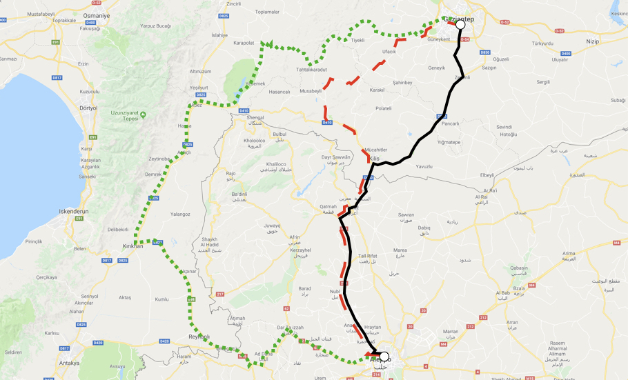
Figure 1. Motivating example.

In many real-world scenarios though, apart from ensuring the diversity of the recommended routes, the collective length, i.e., the total distance covered by vehicles, must also be taken into account to minimize the overall cost. Consider the scenario of transportation of humanitarian aid goods through unsafe regions. The distribution of the load to several vehicles that follow routes dissimilar can increase the chances that at least some of the goods will be delivered. The total distance covered by the vehicles must also be taken into account to minimize the overall cost. For example, Figure 1 shows three different paths from the city of Gaziantep in Turkey to the city of Aleppo in Syria. The solid/black line indicates the shortest path, the dashed/red line the next path in length order, and the dotted/green line a path that is clearly longer, but also significantly different from the other two. Choosing the black and the red paths is not the best option, since the two paths share a large stretch. Among the other two options, the black-green pair has the minimum collective length and, hence, it is a better option than the red-green pair.

The aforementioned scenario is formally captured by the $k$-Dissimilar Paths with Minimum Collective Length ($k\text{DPwML}$) problem. Given two locations $s$ and $t$ on a road network, a $k\text{DPwML}$ query computes a set of $k$ paths from $s$ to $t$ such that: (1) all paths in the result set are sufficiently dissimilar to each other (w.r.t. a user-defined similarity threshold), and (2) the set exhibits the lowest collective path length among all sets of $k$ sufficiently dissimilar paths. $k\text{DPwML}$ was originally introduced by Liu et al. (liu2017, ) as the Top-$k$ Shortest Paths with Diversity (Top-KSPD), together with a greedy heuristic method that builds on the $K$-shortest paths (yen1971, ).

In this paper, we present an in-depth analysis of the $k\text{DPwML}$ problem. First, we conduct a theoretical analysis to prove that $k\text{DPwML}$ is strongly $NP$-hard. Second, we investigate the exact computation of $k\text{DPwML}$ queries, which was not covered by Liu et al. (liu2017, ). We present an algorithm that, similar to the approach of Liu et al., builds on the computation of the $K$-shortest paths (yen1971, ), along with a pair of pruning techniques. Since such approaches require a prohibitively high number of paths to be examined, we introduce the much smaller set of simple single-via paths, which extends the concept of single-via paths (abraham2013, ). Then, we present two algorithms that iterate over this set of paths to compute $k\text{DPwML}$ queries. Our experiments show that algorithms which iterate over all possible $s{-}t$ paths cannot scale. Instead, iterating over the set of simple single-via paths can lead to scalable solutions with a very small trade-off in the quality of the results.

The rest of the paper is organized as follows. In Section 2 we discuss the related work. In Section 3 we introduce the necessary notation, we formally define the $k\text{DPwML}$ problem and we show that the problem is strongly $NP$-hard. In Section 4 we present our exact algorithm along with two pruning techniques. In Section 5 we introduce the concept of simple single-via paths and we present two heuristic algorithms that use simple single-via paths to evaluate $k\text{DPwML}$ queries. Finally, in Section 6 we present the results of our experimental evaluation, and Section 7 concludes this work.

2. Related Work

Different forms of alternative routing have been proposed in the past. Liu et al. (liu2017, ) introduced the problem of finding Top-$k$ Shortest Paths with Diversity ($\mathit{Top{-}KSPD}$), which we study in this paper as the $k\text{DPwML}$. Despite introducing the problem though, Liu et al. investigated only the approximate computation of $k\text{DPwML}$ queries, and they proposed the greedy heuristic algorithm FindKSPD, that builds upon the computation of the $K$-Shortest Paths (yen1971, ), while employing two pruning criteria to limit the number of examined paths. According to the first criterion, partially expanded paths to the same node $n$ are grouped together and the most promising ones are expanded first. The second pruning criterion involves the computation of lower bounds either based on the estimated length or on the similarity of paths to prioritize the examination of paths that are more likely to lead to a solution.

Another way to compute dissimilar alternative routes is to solve the $k$-Shortest Paths with Limited Overlap ($k\text{SPwLO}$) problem, introduced by Chondrogiannis et al. (chondrogiannis2015, ). A $k\text{SPwLO}$ query aims at computing paths that are (a) the shortest path is always included and (b) every new path added to the set is alternative to all the shorter paths already in the set and as short as possible. The authors proposed both exact and heuristic algorithms (chondrogiannis2015, ; chondrogiannis2017, ) to process $k\text{SPwLO}$ queries, using the path overlap (abraham2013, ) as similarity measure. In practice, the greedy FindKSPD algorithm introduced by Liu et al. (liu2017, ) for the $k\text{DPwML}$ is, unbeknownst to the authors, an exact algorithm for the $k\text{SPwLO}$ for arbitrary similarity measures, similar to the baseline approach of Chondrogiannis et al. (chondrogiannis2015, ). Consequently, the $k\text{SPwLO}$ can be seen as an approximation to the $k\text{DPwML}$.

A similar approach to $k\text{SPwLO}$ has been proposed by Jeong et al. (jeong2009, ), that is laxly based on Yen’s algorithm (yen1971, ). At each step, the algorithm modifies each previously computed path to construct a set of candidate paths and examines the one that is most dissimilar to the already recommended paths. Akgun et al. (akgun2000, ) proposed a penalty-based method that doubles the weight of each edge that lies on some already recommended path. The alternative paths are computed by repeatedly running Dijkstra’s algorithm on the input road network, each time with the updated weights. The shortcoming of this approach is that there is no intuition behind the value of the penalty applied before each subsequent iteration. Lim et al. proposed a similar penalty-based approach (lim2005, ) where the penalty is computed in terms of both the path overlap and the total turning cost, i.e., how many times the user has to switch between roads when following a path. In contrast to the $k\text{DPwML}$ and the $k\text{SPwLO}$, neither approach of Jeong et al. nor the penalty-based methods of Akgun et al. and Lim et al. come with an optimization criterion w.r.t. the length of the alternative paths.

A different approach to alternative routing involves methods that focus on computing alternatives only to the shortest paths. Such methods first compute a large set of candidate paths, and then determine the final result set by examining the paths with respect to a number of user-defined constraints. The Plateaux method (cambridge2005, ) aims at computing paths that cross different highways of the road network. Bader et al. (bader2011, ), introduced the concept of alternative graphs which have a similar functionality as the plateaus. Abraham et al. (abraham2013, ) introduced the notion of single-via paths, a set that we extend for developing our heuristic algorithms. The approach of Abraham et al. evaluates each single-via path individually by comparing it to the shortest path, and checks whether each path meets a set of user-defined constraints, i.e., length, local optimality and stretch. Xie et al. (xie2012, ) define alternative paths to the shortest path using edge avoidance, i.e., given an edge of $e$ of the shortest path from $s$ to $t$, the alternative path is the shortest path from $s$ to $t$ which avoids $e$, and introduce iSQPF, a quadtree-based spatial data structure inspired by (samet2008, ). In contrast to our work, none of the aforementioned methods aims at minimizing the collective length of the result set, or guarantees that the result paths will be dissimilar to each other.

Finally, the task of alternative routing can also be based on the pareto-optimal paths for multi-criteria networks (delling2009, ; kriegel2010, ; mouratidis2010, ; shekelyan2015, ). The pareto-optimal paths or the route skyline can be directly seen as alternative routes to move from source node $s$ to target node $t$ or can be further examined in a post-processing phase to provide the final alternative paths. However, our definition of alternative routing is not a multi-criteria problem and the $k\text{SPwLO}$ cannot be obtained by first computing the pareto-optimal path set.

3. Preliminaries

Section 3.1 introduces the necessary notation while Section 3.2 formally defines the $k\text{DPwML}$ problem and Section 3.3 analyzes its complexity.

3.1. Notation

Let $G=(N,E)$ be a directed weighted graph representing a road network with a set of nodes $N$ and a set of edges $E\subseteq N\times N$. Each edge $(n_{i},n_{j})\in E$ is assigned a positive weight $w(n_{i},n_{j})$, which captures the cost of moving from node $n_{i}$ to node $n_{j}$. A (simple) path $p(s{\rightarrow}t)$ from a source node $s$ to a target node $t$ is a connected and cycle-free sequence of edges $\langle(s,n_{i}),\ldots,(n_{j},t)\rangle$. The length $\ell(p)$ of a path $p$ is the sum of the weights of all contained edges, and the collective path length $\mathcal{L(P)}$ of set of paths $P$ is the sum of the lengths of the paths in the set.The length $\ell(p)$ of a path $p$ is the sum of the weights of all contained edges, i.e.,

$$\ell(p)=\sum_{\forall(n_{i},n_{j})\in p}w(n_{i},n_{j})$$

We denote by $\mathcal{L}$ the collective path length for a set of paths $P$, i.e.,

$$\mathcal{L}(P)=\sum_{\forall p\in P}{\ell(p)}$$

The shortest path $p_{sp}(s{\rightarrow}t)$ is the path with the lowest length among all paths that connect $s$ to $t$.

Let $p$, $p^{\prime}$ be two paths between nodes $s$, $t$. We denote the similarity of the paths as $Sim(p,p^{\prime})$. Given a similarity threshold $\theta$, we say that paths $p$, $p^{\prime}$ are sufficiently dissimilar if $Sim(p,p^{\prime})<\theta$. We also say that a path $p$ is sufficiently dissimilar to a set of paths $P$ w.r.t. a threshold $\theta$, if $p$ is sufficiently dissimilar with every path in $P$.

In the past, various measures have been proposed to compute path similarity (cf. (liu2017, )). Choosing the proper similarity measure heavily depends on the application and hence is out of the scope of our work. Nevertheless, the algorithms we present operate with any arbitrary similarity measure. Hence, without loss of generality, we use the Jaccard coefficient, i.e.,

$$Sim(p,p^{\prime})=\frac{\sum_{\forall(n_{i},n_{j})\in p\cap p^{\prime}}w(n_{i},n_{j})}{\sum_{\forall(n_{i},n_{j})\in p\cup p^{\prime}}w(n_{i},n_{j})}$$

Table 1 summarizes the notation used throughout this paper.

Table 1. Summary of notation.

Notation	Description
$G=(N,E)$	Graph $G$ with nodes $N$ and edges $E$
$n$	Node in $N$
$(n_{i},n_{j})$	Edge from node $n_{i}$ to node $n_{j}$
$w(n_{i},n_{j})$	Weight of edge $(n_{i},n_{j})$
$p=\langle(s,n_{1}),\dots,(n_{k},t)\rangle$	Path $p$ from node $s$ to node $t$
$\ell(p)$	Length of path $p$
$\mathcal{L}(P)$	Collective length for a set of paths $P$
$Sim(p,p^{\prime})$	Similarity between two paths $p$ and $p^{\prime}$

Example 3.1.

Consider the road network in Figure 2. The shortest path between nodes $s$ and $t$ is $p_{1}{=}p_{sp}{=}\langle(s,n_{3}),(n_{3},n_{5}),(n_{5},t)\rangle$ with length $\ell(p_{1})=8$. Let $p_{2}=\langle(s,n_{3}),(n_{3},n_{5}),(n_{5},n_{4}),(n_{4},t)\rangle$ and $p_{3}{=}\langle(s,n_{3}),$ $(n_{3},n_{4}),(n_{4},t)\rangle$ be two more paths that connect $s$ to $t$ with length $\ell(p_{2}){=}9$ and $\ell(p_{3}){=}10$, respectively. Assuming a similarity threshold $\theta{=}0.5$, paths $p_{1}$ and $p_{2}$ are not sufficiently dissimilar to each other as their similarity exceeds $\theta$, i.e., $Sim(p_{1},p_{2}){=}6/11\approx 0.545>\theta$ due to the shared edges $(s,n_{3})$ and $(n_{3},n_{5})$. In contrast, paths $p_{3}$ and $p_{1}$ that share only edge $(s,n_{3})$ are sufficiently dissimilar, i.e., $Sim(p_{1},p_{3}){=}3/15{=}0.2<\theta$.

Figure 2. Running example.

3.2. Problem Definition

We now formally restate the problem of finding Top-$k$ Shortest Paths with Diversity (liu2017, ) as the $k$-Dissimilar Paths with Minimum (Collective) Length ($k\text{DPwML}$), using the terminology of Section 3.1.

Problem 1 ($k\text{DPwML}$).

Given a road network $G=(N,E)$, a source $s$ and a target node $t$ both in $N$, a number of requested paths $k$, and a similarity threshold $\theta$, find the $P_{k\text{DPwML}}$ set of paths from $s$ to $t$, such that:

1. all paths in $P_{k\text{DPwML}}$ are pairwise sufficiently dissimilar,

   $$\forall p_{i},p_{j}\in P_{k\text{DPwML}}\text{, }i\neq j:Sim(p_{i},p_{j})<\theta,$$

2. $|P_{k\text{DPwML}}|\leq k$ and $P_{k\text{DPwML}}$ has the maximum possible cardinality among every set of paths $P_{A}$ that satisfy Condition (A),

   $$|P_{k\text{DPwML}}|=\arg\max_{P_{A}}|P_{A}|\text{, and}$$

3. $P_{k\text{DPwML}}$ has the lowest collective path length among every set of paths $P_{AB}$ that satisfy both Conditions (A) and (B),

   $$P_{k\text{DPwML}}=\arg\min_{P_{AB}}\mathcal{L}(P_{AB}).$$

Intuitively, a $k\text{DPwML}$ query returns the maximal set of at most $k$ sufficiently dissimilar paths w.r.t. threshold $\theta$, which have the lowest collective length among all sets of sufficiently dissimilar $s{\rightarrow}t$ paths.

Example 3.2.

Consider again the example in Figure 2 and paths

$$p_{1}=p_{sp} =\langle(s,n_{3}),(n_{3},n_{5}),(n_{5},t)\rangle$$

$$p_{2} =\langle(s,n_{3}),(n_{3},n_{5}),(n_{5},n_{4}),(n_{4},t)\rangle$$

$$p_{3} =\langle(s,n_{3}),(n_{3},n_{4}),(n_{4},t)\rangle$$

$$p_{4} =\langle(s,n_{2}),(n_{2},n_{3}),(n_{3},n_{5}),(n_{5},t)\rangle$$

Let $P_{1}=\{p_{1},p_{2},p_{3}\}$, $P_{2}=\{p_{1},p_{3},p_{4}\}$, and $P_{3}=\{p_{2},p_{3},p_{4}\}$ be three sets of paths with $\mathcal{L}(P_{1})=27$, $\mathcal{L}(P_{2})=29$, and $\mathcal{L}(P_{3})=30$. Consider the query $k\text{DPwML}(s,t,3,0.5)$. While set $P_{1}$ has the lowest collective length, it cannot be the result set as $p_{1}$ and $p_{2}$ are not sufficiently dissimilar, i.e., $Sim(p_{1},p_{2})=6/11=0.545>\theta$. On the other hand, both $P_{2}$ and $P_{3}$ contain sufficiently dissimilar paths, but $P_{2}$ is preferred as $\mathcal{L}(P_{2})<\mathcal{L}(P_{3})$. In fact, $P_{2}$ is the set with the lowest collective length among all sets that contain three sufficiently dissimilar paths. Hence, $P_{2}$ is the result of the query.

3.3. Complexity

We now elaborate on the complexity of the $k\text{DPwML}$ problem. Liu et al. proved in (liu2017, ) (cf. Lemma 1) the $NP$-hardness of $k\text{DPwML}$. Despite the correctness of their finding, the authors’ approach on the proof is incorrect as they polynomially reduced $k\text{DPwML}$ to a hard problem, i.e., the Maximum Independent Set problem, instead of providing a polynomial reduction from a hard problem (arora2009, ). In view of this, we hereby prove the following theorem.

Theorem 3.3.

The $k\text{DPwML}$ problem is strongly $NP$-hard.

Proof.

We prove the lemma by polynomial reduction from the two edge-disjoint path problem in directed graphs ($2$-DP), which is known to be strongly $NP$-complete (eilam-tzoreff1998, ). Given a directed graph $G=(N,E)$ with $|N|=n$ and two source-target pairs $\{s_{1},t_{1}\}$ and $\{s_{2},t_{2}\}$, $2$-DP asks to correctly decide if $G$ contains edge-disjoint paths from $s_{i}$ to $t_{i}$ for $i=1,2$. For polynomially reducing $2$-DP to the task of answering $k\text{DPwML}$ queries, we we define a road network $G^{\prime}=(N^{\prime},E^{\prime})$ with $N^{\prime}=N\cup\{s,t,a,b,c,d\}$ and $E^{\prime}=E\cup\{(s,a),(s,c),(a,b),(c,d),(b,s_{1}),(d,s_{2}),(t_{2},a),(t_{1},c),(b,t),(d,t)\}$. We set $k=4$, $\theta=(2n+1)/(4n^{2}+5)$, $w(e)=4n$ for all $e\in E$, and $w(e)=1$ for all $e\in E^{\prime}\setminus E$. Cf. Figure 3 for a visualization of the network $G^{\prime}$. We claim that there are edge-disjoint paths from $s_{i}$ to $t_{i}$ in $G$ just in case the result of a $4$-DPwML query against $G^{\prime}$ has cardinality $4$. This implies that, unless $P=NP$, there can be no polynomial or pseudo-polynomial algorithm for answering $k\text{DPwML}$ queries.

Figure 3. The network $G^{\prime}$ used for proving that $k\text{DPwML}$ is $NP$-hard. All visualized edges have weight $1$ and the edges contained in the sub-graph $G$ have weight $4n$, where $n$ is the size of $G$.

For proving the claim, we make use of the fact that the similarity of paths $p^{\prime}_{i}(s{\rightarrow}t)$ and $p^{\prime}_{j}(s{\rightarrow}t)$ can be expressed as follows:

(1) $$Sim(p^{\prime}_{i},p^{\prime}_{j})=\frac{\overbrace{\sum_{e\in(p^{\prime}_{i}\cap p^{\prime}_{j})\cap E}w(e)}^{A(p^{\prime}_{i},p^{\prime}_{j})}+\overbrace{\sum_{e\in(p^{\prime}_{i}\cap p^{\prime}_{j})\setminus E}w(e)}^{B(p^{\prime}_{i},p^{\prime}_{j})}}{\underbrace{\sum_{e\in(p^{\prime}_{i}\cup p^{\prime}_{j})\cap E}w(e)}_{C(p^{\prime}_{i},p^{\prime}_{j})}+\underbrace{\sum_{e\in(p^{\prime}_{i}\cup p^{\prime}_{j})\setminus E}w(e)}_{D(p^{\prime}_{i},p^{\prime}_{j})}}$$

We first assume that there are edge-disjoint paths $p_{1}=\langle s_{1},\ldots,t_{1}\rangle$ and $p_{2}=\langle s_{2},\ldots,t_{2}\rangle$ in $G$. Consider the following paths in $G^{\prime}$ $p^{\prime}_{1}=\langle s,a,b,p_{1},c,d,t\rangle$, $p^{\prime}_{2}=\langle s,c,d,p_{2},a,b,t\rangle$, $p^{\prime}_{3}=\langle s,a,b,t\rangle$, and $p^{\prime}_{4}=\langle s,c,d,t\rangle$. Then the following statements immediately follow from the construction of $G^{\prime}$:

1. Since paths $p_{1}$ and $p_{2}$ are edge disjoint, we have $A(p^{\prime}_{i},p^{\prime}_{j})=0$ for all $(i,j)\in\{1,\ldots,4\}\times\{1,\ldots,4\}$.

2. We have $B(p^{\prime}_{3},p^{\prime}_{4})=0$ and $B(p^{\prime}_{i},p^{\prime}_{j})=2$ for all $(i,j)\in\{1,\ldots,4\}\times\{1,\ldots,4\}\setminus\{(3,4),(4,3)\}$.

3. Since the paths $p_{1}$ and $p_{2}$ use at least one edge in $E$, we have $C(p^{\prime}_{i},p^{\prime}_{4})\geq 4n$ for all $(i,j)\in\{1,\ldots,4\}\times\{1,\ldots,4\}\setminus\{(3,4),(4,3)\}$.

4. We have $D(p^{\prime}_{i},p^{\prime}_{4})\geq 7$ for all $(i,j)\in\{1,\ldots,4\}\times\{1,\ldots,4\}\setminus\{(3,4),(4,3)\}$.

These statements imply that, for all $(i,j)\in\{1,\ldots,4\}\times\{1,\ldots,4\}$, we have $Sim(p^{\prime}_{i},p^{\prime}_{j})\leq 2/(4n+7)<(2n+1)/(4n^{2}+5)=\theta$, and hence, that $P_{k\text{DPwML}}=\{p^{\prime}_{i}\}^{4}_{i=1}$ is a result set for $4$-DPwML with cardinality four.

For the other direction of the claim, assume that there is a set $P_{k\text{DPwML}}=\{p^{\prime}_{i}\}^{4}_{i=1}$ of four paths from $s$ to $t$ in $G^{\prime}$ with pairwise similarity less than $\theta=(2n+1)/(4n^{2}+5)$. By construction of $G^{\prime}$, we know that each path either starts with the prefix $\mathit{prefix}_{1}=\langle(s,a),(a,b)\rangle$ or with the prefix $\mathit{prefix}_{2}=\langle(s,c),(c,d)\rangle$. Furthermore, we can see that a path $p^{\prime}_{i}(s{\rightarrow}t)$ that starts with $\mathit{prefix}_{1}$ either equals $\langle(s,a),(a,b),(b,t)\rangle$ or, at node $b$, enters $G$ through the edge $(b,s_{1})$. Assume that the latter is the case. Then we know that $p^{\prime}_{i}$ exits $G$ through the edge $(t_{1},c)$, since exiting $G$ through $(t_{2},a)$ would close the cycle $\langle(a,b),(b,s_{1})(s_{1},\ldots),(\ldots,t_{2}),(t_{2},a)\rangle$ and hence contradict the fact that $p^{\prime}_{i}$ is a path. Therefore, $p^{\prime}_{i}$ starts with the prefix $\mathit{prefix}_{1}=\langle(s,a),(a,b),(b,s_{1}),\ldots,(t_{1},c),(c,d)\rangle$. At node $d$, $p^{\prime}_{i}$ cannot enter $G$ again, since both exit edges $(t_{1},c)$ and $(t_{2},a)$ would close a cycle. This implies that $p^{\prime}_{i}=\langle s,a,b,s_{1},\ldots,t_{1},c,d,s\rangle$. Analogously, we can show that a path $p^{\prime}_{i}(s{\rightarrow}t)$ that starts with $\mathit{prefix}_{2}$ either equals $\langle(s,c),(c,d),(d,t)\rangle$ or is of the form $p^{\prime}_{i}=\langle(s,c),(c,d),(d,s_{2}),(s_{2},\ldots),(\ldots,t_{2}),(t_{2},a),(a,b),(b,s)\rangle$.

These observations imply that $P_{k\text{DPwML}}$ contains paths $p^{\prime}_{1}=\langle(s,a),(a,b)\rangle\cdot p_{1}\cdot\langle(c,d)(d,s)\rangle$, $p^{\prime}_{2}=\langle(s,c),(c,d)\rangle\cdot p_{2}\cdot\langle(a,b),(b,s)\rangle$, $p^{\prime}_{3}=\langle(s,a),(a,b),(b,t)\rangle$, and $p^{\prime}_{4}=\langle(s,c),(c,d),(d,t)\rangle$, where $p_{i}$ are paths from some $s_{i}$ to some $t_{i}$ in $G$. It remains to be shown that $p_{1}$ and $p_{2}$ are edge-disjoint. Assume that this is not the case. Then the following statements hold:

1. Since $p_{1}$ and $p_{2}$ share at least one edge from $E$, we have $A(p^{\prime}_{1},p^{\prime}_{2})\geq 4n$.

2. Since $p^{\prime}_{1}$ and $p^{\prime}_{2}$ share exactly two edges from $E^{\prime}\setminus E$, we have $B(p^{\prime}_{1},p^{\prime}_{2})=2$.

3. Since both $p_{1}$ and $p_{2}$ contain at most $n$ edges from $E$, we have $C(p^{\prime}_{1},p^{\prime}_{2})\leq 8n^{2}$.

4. Since each edge from $E^{\prime}\setminus E$ is contained in $p^{\prime}_{1}$ or in $p^{\prime}_{2}$, we have $D(p^{\prime}_{1},p^{\prime}_{2})=10$.

This statements imply that

$$Sim(p^{\prime}_{1},p^{\prime}_{2})\geq(4n+2)/(8n^{2}+^{0})=(2n+1)/(4n^{2}+5)=\theta$$

which contradicts the fact that $Sim(p^{\prime}_{1},p^{\prime}_{2})<\theta$. Therefore, $p_{1}$ and $p_{2}$ are edge-disjoint, which yields the claim and finishes the proof of the theorem. ∎

4. An Exact Approach

(a) Subsets of $P=\{p_{1},p_{2},p_{3}\}$.

(b) Subsets of $P=\{p_{1},p_{2},p_{3},p_{4}\}$.

Figure 4. Binomial trees for generating subsets of paths with cardinality up to 3.

A naïve approach for an exact solution to $k\text{DPwML}$ would first identify all paths from a source node $s$ to a target node $t$ and examine all possible sets of at most $k$ paths to determine the set that satisfies the conditions of Problem 1. Such an approach is clearly impractical. In view of this, Section 4.1 defines a pair of pruning techniques, and Section 4.2 presents an exact algorithm that employs these techniques to reduce the search space during $k\text{DPwML}$ query processing.

4.1. Pruning Techniques

Lower Bound on Collective Path Length

Our first pruning technique employs a lower bound on the collective path length, which limits the total number of paths to be constructed. Let $P_{all}$ be the set of all possible paths from node $s$ to $t$, and $p^{*}_{i}$ be the $i$-shortest path in $P_{all}$ (i.e., $p^{*}_{1}=p_{sp}$). Then, for every path $p$ in $P_{all}$, the collective path length of every $k$-subset $P\subset P_{all}$ that contains $p$ is lower bounded as follows:

(2) $$\mathcal{L}(P)\geq\ell(p)+\sum_{i=1}^{k{-}1}\ell(p^{*}_{i})$$

Intuitively, the right part of the above inequality defines a set of paths that contain $p$ and the $(k{-}1)$ shortest paths in $P_{all}$; by definition, such a set should have the lowest collective path length compared to any subset of $P_{all}$ that includes $p$.

We can use the lower bound of Inequality 2 to exclude a path $p$ from the result set of $P_{k\text{DPwML}}$. The idea is captured by the following lemma:

Lemma 4.1.

Let $P_{all}$ be the set of all paths from $s$ to $t$, $P_{A}\subseteq P_{all}$ be a set of $k$ paths that satisfy Condition (A) of Problem 1, i.e., the contained paths are sufficiently dissimilar to each other, and $P^{*}_{k-1}$ be the set of the $k-1$ shortest paths in $P_{all}$. A path $p\in P_{all}\setminus P_{A}$ cannot be part of the $k\text{DPwML}$ result if $\mathcal{L}(\{p\}\cup P^{*}_{k-1})>\mathcal{L}(P_{A})$.

Proof.

By definition, $P^{*}_{k-1}$ is the set of $k{-}1$ paths with the minimum possible collective length among all subsets containing $k{-}1$ paths. Hence, the subset $P$ which contains $p$ and achieves the least possible path length sum is $P=P^{*}_{k-1}\cup\{p\}$. Therefore, if there exists a set of sufficiently dissimilar paths $P_{A}$, i.e., $\forall p_{i},p_{j}\in P_{A}$, $i\neq j:Sim(p_{i},p_{j})<\theta$, $p\not\in P_{A}$ and $\mathcal{L}(P_{A})<\mathcal{L}(P)$, then the path length sum of any set $P^{\prime}$ with $p\in P^{\prime}$ will be greater than the path length sum of $P_{A}$. Consequently, there exist no set of at most $k$ dissimilar paths, which contains $p$ (or any path longer than $p$), and achieves a collective length smaller that $\mathcal{L}(P_{A})$. ∎

With Lemma 4.1, when processing a $k\text{DPwML}$ query, it suffices to construct paths from source node $s$ to target node $t$ in increasing length order and use the lemma as a termination condition. If the next path $p$ in length order cannot be part of the final result set, then the current set of paths achieves the lowest possible path length and, hence, it is the final $P_{k\text{DPwML}}$ result.

Excluding Subsets of Similar Paths

Our second pruning technique prevents the construction of path sets that do not exclusively contain sufficiently dissimilar paths. The key idea behind this technique is to incrementally generate the path sets by reusing already generated smaller subsets. For this purpose, we employ a dynamic programming scheme named ”filling a rucksack” or Algorithm $F$ for simplicity (knuthTAOCP, ), that builds on the concept of binomial trees. Given a set of paths $P$, we use a binomial tree $T$ of height $k$ to represent all subsets $P_{i}\subseteq P$ of cardinality $|P_{i}|\leq k$. Each time a new path $p^{\prime}$ is added to set $P$, Algorithm $F$ extends all existing subsets of cardinality up to $k{-}1$ to generate the subsets of cardinality up to $k$ that contain $p^{\prime}$. More specifically, a new branch is attached to the root of the binomial tree using an edge labeled by $p^{\prime}$, and the subtree representing subsets of cardinality up to $k{-}1$ is added under the new branch. Note that during this expansion phase, the height of the binomial tree remains fixed but the tree becomes wider.

Example 4.2.

Consider the example in Figure 4. Figure 4a illustrates the binomial tree of height $k{=}3$ for the path set $P=\{p_{1},p_{2},p_{3}\}$. The leaf nodes of the tree represent all possible subsets of $P$ containing at most $k{=}3$ paths. Also, the subtree $T_{1}$ (indicated with blue lines) represents all possible subsets of $P$ of cardinality up to $k{-}1=2$. Then, Figure 4b illustrates the expanded binomial tree after adding a new path $p_{4}$ to $P$. Observe the new branch attached to the root node via the edge representing $p_{4}$. Also, the subtree $T_{2}$ attached under the new branch (also indicated with blue lines) is identical to subtree $T_{1}$.

During the execution of Algorithm F, instead of generating the contents of each new branch from scratch, the algorithm simply copies the subtree that represents all subsets of cardinality up to $k{-}1$ before adding the new path. Consequently, when computing a $k\text{DPwML}$ query, it suffices to apply Algorithm $F$ to incrementally generate new subsets of paths and early prune subsets that contain at least one pair of not sufficiently dissimilar paths. In Figure 4 for example, assume that the similarity of paths $p_{1}$ and $p_{2}$ exceeds the given threshold $\theta$, i.e., $Sim(p_{1},p_{2})>\theta$. That is, the paths are not sufficiently dissimilar and consequently, no subset containing paths $p_{1}$ and $p_{2}$ can be part of the $k\text{DPwML}$ result. In this case, the branch representing the $\{p_{1},p_{2}\}$ subset indicated by the dashed line is excluded from every subtree of the binomial tree and hence, all subsets that contain both $p_{1}$ and $p_{2}$ are never generated.

Figure 5. $K$SP-DML computing $k\text{DPwML}(s,t,3,0.5)$; result paths highlighted in light gray.

4.2. The $K$SP-DML Algorithm

We now present our exact $K$SP-DML algorithm for $k\text{DPwML}$, which employs the pruning techniques discussed in Section 4.1. The algorithm builds upon the computation of the $K$-Shortest Paths (yen1971, ), with the goal to progressively compute the exact solution. At each round, $K$SP-DML employs Algorithm $F$ from (knuthTAOCP, ) to generate subsets of at most $k$ paths. Using our second pruning technique, subsets that violate the similarity constraint are filtered out. The algorithm examines only the subsets with the largest possible cardinality and, among those, only the one with the lowest collective path length is retained. $K$SP-DML uses our first pruning technique as the termination condition, i.e., the algorithm terminates after a path that satisfies the criterion of Lemma 4.1 is constructed.

Algorithm 1 illustrates the pseudocode of our exact $K$SP-DML algorithm, which employs the two aforementioned pruning techniques. All generated shortest paths are stored in set $P_{sp}$. In Line 2, we set $p$ as the first shortest path from $s$ to $t$. From Line 3 to 11, $K$SP-DML iterates over the next shortest path starting from the first one. In Line 4, current path $p$ is stored in $P_{sp}$. In Lines 5–6, the collective length $\mathcal{L}_{k{-}1}$ of the first $k{-}1$ shortest paths is computed to be used for the lower bound in Line 3. Next, Algorithm $F$ (knuthTAOCP, ) is called in Line 7 to determine all $(\leq k)$-subsets $P$ of $P_{sp}$ that contain $p$. For each subset $P$, Line 8 checks whether all paths in $P$ are sufficiently dissimilar to each other (Condition (A) of Problem 1). Subsequently, Line 9 checks whether $P$ contains more paths than $P_{k\text{DPwML}}$ (Condition (B) of Problem 1), or $P$ contains as many paths as $P_{k\text{DPwML}}$ and has a lower collective length than current $P_{k\text{DPwML}}$ (Conditions (B) and (C) of Problem 1). If either case holds, $K$SP-DML updates the $P_{k\text{DPwML}}$ result in Line 10. The examination of each next shortest path (and $K$SP-DML overall) terminates when either all possible paths from $s$ to $t$ have been generated or the termination condition of Line 3 is met.

Input: Road network $G=(N,E)$, source node $s$, target node $t$, number of results $k$, similarity threshold $\theta$

Output: Set $P_{k\text{DPwML}}$ of at most k paths

1initialize $P_{sp}\leftarrow\emptyset$, $\mathcal{L}_{k{-}1}\leftarrow 0$, $P_{k\text{DPwML}}\leftarrow\emptyset$, $P\leftarrow\emptyset$;

$p\leftarrow\textnormal{{NextShortestPath}}(G,s,t)$;

  $\triangleright$ Shortest path $p_{sp}$

2while $p{\neq}\mathit{null}$ and ($|P_{k\text{DPwML}}|{<}k$ or $\ell(p){+}\mathcal{L}_{k{-}1}{\leq}\mathcal{L}(P_{k\text{DPwML}})$) do

3       $P_{sp}\leftarrow P_{sp}\cup\{p\}$;

4      if $|P_{sp}|<k$ then

5             $\mathcal{L}_{k{-}1}\leftarrow\mathcal{L}_{k{-}1}+\ell(p)$;

6      foreach $P\subseteq P_{sp}:|P|\leq k$ with $p\in P$ do $\triangleright$ Alg. $F$ (knuthTAOCP, )

7            if $\forall$ $p_{i},p_{j}\in P$ with $i\neq j:Sim(p_{i},p_{j})<\theta$ then $\triangleright$ Problem 1 Condition (A)

8                   if $|P|>|P_{k\text{DPwML}}|$ or                                             $|P|=|P_{k\text{DPwML}}|$ and $\mathcal{L}(P)<\mathcal{L}(P_{k\text{DPwML}})$ then $\triangleright$ Problem 1 Conditions (B), (C)

                         $P_{k\text{DPwML}}\leftarrow P$;

                          $\triangleright$ Update result set

9                        

10                  

11            

12      $p\leftarrow\textnormal{{NextShortestPath}}(G,s,t)$;

13return $P_{k\text{DPwML}}$;

Algorithm 1 $K$SP-DML

Example 4.3.

Figure 5 illustrates the execution of $K$SP-DML for the $k\text{DPwML}(s,t,3,0.5)$ query; on the right-hand side of the figure, we report the $P_{sp}$ set with the examined paths in length order. Initially, the shortest path $p_{1}{=}p_{sp}$ is generated and the result set $P_{k\text{DPwML}}=\{p_{1}=p_{sp}\}$ is initialized. Next, path $p_{2}$ is computed, but since $Sim(p_{1},p_{2})=0.545>0.5$ subset $\{p_{1},p_{2}\}$ is never constructed. At this point though, $\mathcal{L}_{k{-}1}=8+9=17$ is computed. Then, the algorithm computes the next shortest path in length order, i.e., $p_{3}$. The computation of $p_{3}$ results in no sets of $k$ sufficient dissimilar paths. In fact, there exists a single subset $\{p_{1},p_{2},p_{3}\}$ of $P_{all}$ that contains $p_{3}$ but it is never constructed as $Sim(p_{1},p_{2})>\theta$. In contrast, there exists set $P_{1}=\{p_{2},p_{3}\}$ which contains sufficiently dissimilar paths and $|P_{1}|>|P_{k\text{DPwML}}|$. Hence, $P_{k\text{DPwML}}$ is updated, i.e., $P_{k\text{DPwML}}=P_{1}$. Next, the 4th shortest path $p_{4}$ is generated and subsets $P_{2}=\{p_{1},p_{3},p_{4}\}$ and $P_{3}=\{p_{2},p_{3},p_{4}\}$ are constructed both containing more sufficiently dissimilar paths than the current result. Since $P_{2}$ has the lowest collective length, i.e., $\mathcal{L}(P_{2})=29$, it becomes the temporary result set, i.e. $P_{k\text{DPwML}}=P_{2}$. The algorithm continues its execution as $\ell(p_{4})+\mathcal{L}_{k{-}1}>\mathcal{L}(\{p_{1},p_{3},p_{4}\})$ (Lemma 4.1). Note that, since a temporary result of $k$ sufficiently paths has been found, there is no need to examine subsets of less than $k$ paths from now on. The subsequent generation of paths $p_{5}$ and $p_{6}$ result in the construction of subsets none of which achieve lower collective length that $P_{2}$. However, the algorithm terminates only when the 7th shortest path $p_{7}$ is retrieved, for which $\ell(p_{7})+\mathcal{L}_{k{-}1}\geq\mathcal{L}(P_{2})$ and so, the final result $P_{k\text{DPwML}}=P_{2}=\{p_{1},p_{3},p_{5}\}$ is returned.

Complexity Analysis

In the worst case, $K$SP-DML has to examine all $\binom{K}{k}$ subsets containing $k$ $(s{\rightarrow}t)$ paths, where $K$ is the number of all paths from $s$ to $t$ that the algorithm needs to examine. Even for $k=O(1)$, the best complexity guarantee one can give for $K$SP-DML is hence $O(\operatorname*{poly}(K))$. Since $K$ is not polynomially bounded in the size of the network $G$, this is prohibitively expensive. In fact, $K$ is usually very large; for random graphs with density $d$, the expected value is $\mathbb{E}(K)=\Omega((|N|-2)!d^{|N|})$ (roberts2007, ).

5. Heuristic Approaches

Our complexity analysis in Section 4.2 showed that the cost of $K$SP-DML is prohibitively high due to the number $K$ of paths that need to be examined; in practice, we expect this $K$ to be significantly larger than the requested number of results $k$. Consequently, solutions that build on the computation of the $K$-shortest paths, i.e., both our exact $K$SP-DML and the heuristic FindKSPD algorithm of Liu et al. (liu2017, ), cannot scale to real-world road networks. In this spirit, Section 5.1 introduces the concept of simple single-via paths which allow us to drastically reduce the search space. Then, Sections 5.2 and 5.3 present our heuristic algorithms for the $k\text{DPwML}$ problem that iterate over the set of simple single-via paths in length order.

5.1. Simple Single-Via Paths

The concept of single-via paths (SVP) initially proposed by Abraham et al. (abraham2013, ) and then optimized by Luxen and Schieferdecker (luxen2015, ), has been primarily used for alternative routing on road networks (abraham2013, ; luxen2015, ; chondrogiannis2017, ). Given a road network $G{=}(N,E)$, a source node $s$ and a target node $t$, the single-via path $p_{sv}(n)$ of a node $n\in N\setminus\{s,t\}$ is defined as $p_{sp}(s{\rightarrow}n)\circ p_{sp}(n{\rightarrow}t)$, i.e., the concatenation of shortest paths $p_{sp}(s{\rightarrow}n)$ and $p_{sp}(n{\rightarrow}t)$. By definition, $p_{sv}(n)$ is the shortest possible path that connects $s$ and $t$ through $n$.

However, using the set of single-via paths to process $k\text{DPwML}$ queries raises two important issues. First, the single-via path $p_{sv}(n)$ of every node $n$ crossed by the shortest path $p_{sp}(s{\rightarrow}t)$ is identical to $p_{sp}$. Computing the single-via paths for these particular nodes is unnecessary. Second, there is no guarantee that a single-via path is simple (i.e., cycle-free), which may result in recommending paths that make little sense from a user perspective. For instance, consider the road network in Figure 6. The single-via path of node $n_{2}$ is $p_{sv}(n_{2}){=}p_{sp}(s{\rightarrow}n_{2})\circ p_{sp}(n_{2}{\rightarrow}t)$, which is clearly not a simple path, i.e., $p_{sv}(n_{2}){=}\langle(s,n_{3}),(n_{3},n_{2}),(n_{2},n_{3}),(n_{3},n_{5}),(n_{5},t)\rangle$.

To address the aforementioned issues, we introduce the simple single-via paths (SSVP). Given a road network $G{=}(N,E)$, a source node $s$ and a target node $t$, the SSVP $p_{ssv}(n)$ of a node $n\in N\setminus\{s,t\}$ is defined only if $n$ does not lie on the shortest path $p_{sp}(s{\rightarrow}t)$. If the single-via path $p_{sv}(n)$ of node $n$ is simple, then $p_{ssv}(n){=}p_{sv}(n)$. Otherwise, $p_{ssv}(n)$ is the concatenation either of $p_{sp}(s{\rightarrow}n)$ with the shortest path $p^{\prime}(n{\rightarrow}t)$ from $n$ to $t$ that visits no nodes in $p_{sp}(s{\rightarrow}n)$, i.e., $sp(s{\rightarrow}n)\circ p^{\prime}(n{\rightarrow}t)$, or the concatenation of the shortest path $p^{\prime}(s{\rightarrow}n)$ from $s$ to $n$ that visits no nodes in $p_{sp}(n{\rightarrow}t)$ with $p_{sp}(n{\rightarrow}t)$, i.e., $p^{\prime}(s{\rightarrow}n)\circ p_{sp}(n{\rightarrow}t)$. In this case, the SSVP of $n$ is the concatenated path with the lowest path length. Note that the shortest path $p_{sp}(s{\rightarrow}t)$ is a SSVP by definition.

Consider again the road network in Figure 2. As mentioned already, the single-via path $p_{sv}(n_{2})$ is not simple. Hence, the simple single-via path $p_{ssv}(n_{2})$ is either $p=\langle(s,n_{2}),(n_{2},n_{3}),(n_{3},n_{5}),(n_{5},t)\rangle$ or $p^{\prime}=\langle(s,n_{n}3),(n_{3},n_{2}),(n_{2},n_{4}),(n_{4},t)\rangle$. In this particular case, both concatenated paths have the same length, i.e., $\ell(p)=\ell(p^{\prime})=11$, and either can be set as $p_{ssv}(n_{2})$. The table on the right-hand side of Figure 6 illustrates the simple single-via paths for the road network of our running example.

5.2. The SSVP-DML Algorithm

A straightforward way of employing SSVPs for processing $k\text{DPwML}$ queries is to alter the exact $K$SP-DML algorithm from Section 4.2 such that the algorithm iterates over the simple single-via paths from source $s$ to target $t$ in increasing length order, instead of retrieving the next shortest path. By the definition of SSVP, the search space will be drastically reduced as at most $|N|{-}1$ paths will be examined. In addition, we can still use the pruning techniques proposed in Section 4.1 to terminate the search and avoid generating candidate path sets that do not contain sufficiently dissimilar paths. Our first heuristic algorithm, termed SSVP-DML, follows this approach. Naturally, as the result of $k\text{DPwML}$ queries may not consist exclusively of simple single-via paths, SSVP-DML can only provide an approximate solution to the $k\text{DPwML}$ problem.

Input: Road network $G=(N,E)$, source node $s$, target node $t$, $\#$ of results $k$, similarity threshold $\theta$

Output: Set $P_{k\text{DPwML}}$ of at most $k$ paths

1initialize $P_{ssv}\leftarrow\emptyset$, $\mathcal{L}_{k{-}1}\leftarrow 0$,$P_{k\text{DPwML}}\leftarrow\emptyset$,$P\leftarrow\emptyset$;

$p\leftarrow\textnormal{{NextSSVPByLength}}(G,s,t)$;

  $\triangleright$ Shortest path $p_{sp}$

2while $p\neq\mathit{null}$ and                                                           ($|P_{k\text{DPwML}}|{<}k$ or $\ell(p){+}\mathcal{L}_{k{-}1}{\leq}\mathcal{L}(P_{k\text{DPwML}})$) do $\triangleright$ Lemma 4.1

3       $P_{ssv}\leftarrow P_{ssv}\cup\{p\}$;

4      if $|P_{ssv}|<k$ then

5             $\mathcal{L}_{k{-}1}\leftarrow\mathcal{L}_{k{-}1}+\ell(p)$;

6      foreach $P\subseteq P_{ssv}:|P|\leq k$ with $p\in P$ do $\triangleright$ Alg. $F$ (knuthTAOCP, )

7            if $\forall$ $p_{i},p_{j}\in P$ with $i\neq j:Sim(p_{i},p_{j})<\theta$ then

8                   if $|P|>|P_{k\text{DPwML}}|$ or                                                  $|P|=|P_{k\text{DPwML}}|$ and $\mathcal{L}(P)<\mathcal{L}(P_{k\text{DPwML}})$ then

                         $P_{k\text{DPwML}}\leftarrow P$;

                          $\triangleright$ Update result set

9                        

10                  

11            

12      $p\leftarrow\textnormal{{NextSSVPByLength}}(G,s,t)$;

13return $P_{k\text{DPwML}}$;

Algorithm 2 SSVP-DML

Algorithm 2 illustrates the pseudocode of SSVP-DML. The algorithm keeps track of all generated simple single-via paths inside set $P_{ssv}$ (instead of the shortest paths inside $P_{sp}$, in Algorithm 1). SSVP-DML proceeds exactly as $K$SP-DML but replaces the call to NextShortestPath by a call to the NextSSVPByLength function, which retrieves the next simple single-via path $p(s{\rightarrow}t)$ in increasing length order. In Line 2, the first simple single-via path, i.e., the $p_{sp}(s\rightarrow t)$ shortest path, is retrieved. From Line 3 to 11, SSVP-DML iterates over each next simple single-via path $p$ in order, to determine the subsets of $P_{ssv}$ that contain $p$ and satisfy the conditions of Problem 1 (Lines 8–9). Upon identifying such subsets the algorithm updates $P_{k\text{DPwML}}$ if needed, in Line 10, similar to $K$SP-DML. Also like $K$SP-DML, SSVP-DML terminates after all simple single-via paths have been examined or if current single simple-via path $p$ satisfies the termination condition of Lemma 4.1.

Next, we elaborate on NextSSVPByLength. We design the function as an iterator which allows us to compute the simple single-via paths in increasing length order. Function 3 illustrates the pseudocode of NextSSVPByLength. Upon the first call (Lines 1–11), the function constructs the shortest path trees $T_{s{\rightarrow}N}$ and $T_{N{\rightarrow}t}$ and the shortest path $p_{sp}$ from $s$ to $t$; note that $T_{N{\rightarrow}t}$ is computed by reversing the direction of the network edges. In addition, all nodes $n$ of the road network that are not crossed by $p_{sp}$ are organized inside min-priority queue $\mathcal{Q}$ according to the length of their single-via path, i.e., $\ell(p_{s{\rightarrow}n}\circ p_{n{\rightarrow}t})$. Note that $\mathcal{Q}$ is static, i.e., its contents are preserved throughout every call of NextSSVPByLength. Last, the shortest path $p_{sp}$ is returned as the first simple single-via path in Line 11. Every followup function call to compute the next simple single-via path in length order, is handled by Lines 12–24. In Line 13 the node at the top of $\mathcal{Q}$ is extracted and, in Line 14, NextSSVPByLength checks whether single-via path $p_{sv}(n)=p_{s{\rightarrow}n}\circ p_{n{\rightarrow}t}$ is simple. If so, then the path is returned. By definition a simple single-via path of a node $v$ is at least as long as the single-via path of $v$, i.e., $\ell(p_{ssv}(n))\geq\ell(p_{sv}(n))$. Thus, as the remaining nodes in $\mathcal{Q}$ have a longer single-via path than top node $n$, the returned path is indeed the next simple single-via path in increasing length order.

If path $p_{s{\rightarrow}n}\circ p_{n{\rightarrow}t}$ is not simple, then function NextSSVPByLength needs to construct the simple single-via path of current node $n$. This construction involves three steps in Lines 17–26. First, the subgraphs $G_{1}$ and $G_{2}$ of the original network are defined by excluding nodes that are crossed by shortest paths $p_{s{\rightarrow}n}$ and $p_{n{\rightarrow}t}$, respectively, in Lines 17–20. Then, in Lines 21–22, the NextSSVPByLength computes paths $p_{1}$ and $p_{2}$, which are the candidate paths for being the simple single-via path of $n$. Note that the shortest paths that are computed on $G_{1}$ and $G_{2}$ instead of the original road network $G$ guarantee that the candidate paths $p_{1}$ and $p_{2}$ are simple. Last, in Lines 23–26, the shortest path among $p_{1}$ and $p_{2}$ is selected as the simple single-via path of current node $n$, and is subsequently inserted to $\mathcal{Q}$. This, step is necessary to guarantee that the function always returns the next simple single-via path in length order. Every call to NextSSVPByLength returns the next simple single-via paths in length order until $\mathcal{Q}$ is empty, i.e., until all simple single-via paths have been generated.

Input: Road network $G(N,E)$, source node $s$, target node $t$

Output: Next simple single-via path by length

1if first call then

2       initialize static min-priority queue $\mathcal{Q}\leftarrow\emptyset$;

3      $T_{s{\rightarrow}N}\leftarrow$ shortest path tree from $s$ to all $n\in N$;

4      $T_{N{\rightarrow}t}\leftarrow$ shortest path tree from all $n\in N$ to $t$;

5      $p_{sp}\leftarrow\textnormal{{ComputeShortestPath}}(G,s,t)$;

6       foreach $n\in N-\{s,t\}$ do

7             if $n$ is not crossed by $p_{sp}$ then

8                   $p_{s\rightarrow n}\leftarrow\textnormal{{RetrieveShortestPath}}(T_{s{\rightarrow}N},s,n)$;

9                  $p_{n\rightarrow t}\leftarrow\textnormal{{RetrieveShortestPath}}(T_{N{\rightarrow}t},n,t)$;

10                  $\mathcal{Q}.push(\langle n,\ell(p_{s\rightarrow n}){+}\ell(p_{n\rightarrow t}),p_{s\rightarrow n}\circ p_{n\rightarrow t}\rangle)$;

11            

12      return $p_{sp}$;

13      

14while $\mathcal{Q}$ is not empty do

15       $\langle n,\ell(p_{s\rightarrow n}\circ p_{n\rightarrow t}),p_{s\rightarrow n}\circ p_{n\rightarrow t}\rangle\leftarrow\mathcal{Q}.pop()$;

16      if $p_{s\rightarrow n}\circ p_{n\rightarrow t}$ is simple then

17             return $p_{s\rightarrow n}\circ p_{n\rightarrow t}$;

18            

19       else

20             let $N_{1}=N\setminus\{$nodes crossed by $p_{s\rightarrow n}\}$ except $s,n$;

21             let $N_{2}=N\setminus\{$nodes crossed by $p_{n\rightarrow t}\}$ except $n,t$;

22             let $E_{1}=E\setminus p_{s\rightarrow n}$;

23             let $E_{2}=E\setminus p_{n\rightarrow t}$;

24             $p_{1}\leftarrow p_{s\rightarrow n}\circ\textnormal{{ComputeShortestPath}}(G_{1}(N_{1},E_{1}),n,t)$;

25            $p_{2}\leftarrow\textnormal{{ComputeShortestPath}}(G_{2}(N_{2},E_{2}),s,n)\circ p_{n\rightarrow t}$;

26            if $\ell(p_{1})\leq\ell(p_{2})$ then

27                   $\mathcal{Q}.push(\langle n,\ell(p_{1}),p_{1}\rangle)$;

28             else

29                   $\mathcal{Q}.push(\langle n,\ell(p_{2}),p_{2}\rangle)$;

30            

31      

32return null;

Function 3 NextSSVPByLength

Figure 6. SSVP-DML and SSVP-D+ computing $k\text{DPwML}(s,t,3,0.5)$; result paths highlighted in light gray.

Example 5.1.

Figure 6 illustrates the execution of SSVP-DML for the $k\text{DPwML}(s,t,3,0.5)$ query. On the right-hand side of the figure we report the set of simple single-via paths $P_{ssv}$ examined by the algorithm in increasing length order. Initially, the first simple single-via path, i.e., the shortest path $p_{sp}$, is retrieved and the result set $P_{k\text{DPwML}}=\{p_{sp}\}$ is initialized. Next, simple single-via path $p_{ssv}(n_{4})$ is retrieved. Since $Sim(p_{sp},p_{ssv}(n_{4})){=}0.545>0.5$ subset $\{p_{sp},p_{ssv}(n_{4})\}$ is never constructed. At this point, $\mathcal{L}_{k{-}1}{=}8{+}9{=}17$ is computed. Then, the next single-via path in length order $p_{ssv}(n_{2})$ is retrieved. The retrieval of $p_{ssv}(n_{2})$ results in no sets of $k$ sufficient dissimilar as the only subset of three paths $\{p_{sp},p_{ssv}(n_{4}),p_{ssv}(n_{2})\}$ is never constructed. Among the subsets containing two paths, set $P_{1}=\{p_{sp},p_{ssv}(n_{2})\}$ has the the lowest collective length, i.e., $\mathcal{L}(P_{1})=19$. Hence, at this point $P_{k\text{DPwML}}$ is set equal to $P_{1}$. Subsequently, the next simple single-via path in length order $p_{ssv}(n_{1})$ is retrieved. The retrieval of $p_{ssv}(n_{1})$ results in the creation of subsets $P_{2}{=}\{p_{sp},p_{ssv}(n_{2}),p_{ssv}(n_{1})\}$ and $P_{3}{=}\{p_{ssv}(n_{4}),p_{ssv}(n_{2}),p_{ssv}(n_{1})\}$. Consequently, as $\mathcal{L}(P_{2})<\mathcal{L}(P_{3})$ the result set $P_{k\text{DPwML}}$ is updated, i.e., $P_{k\text{DPwML}}=P_{2}$. Since there are no more simple single-via paths left to examine, the algorithm terminates.

5.3. The SSVP-D+ Algorithm

Despite reducing the search space compared to $K$SP-DML, SSVP-DML still needs to examine all possible subsets of at most $k$ sufficiently dissimilar paths. The generation of these subsets is accelerated by the use of the binomial trees (as discussed in Section 4.1), but overall we expect this procedure to dominate the evaluation of the $k\text{DPwML}$ query, rendering $K$SP-DML inefficient for real-world networks. In view of this, we devise a second heuristic algorithm, termed SSVP-D+, which adopts a similar idea to FindKSPD and to our previous work (chondrogiannis2015, ; chondrogiannis2017, ). The algorithm constructs progressively an approximate solution to $k\text{DPwML}$ that (1) always contains the shortest path from source node $s$ to target $t$ and (2) every newly added path to the result set is both sufficiently dissimilar to the previously recommended paths and as short as possible. As discussed in Section 2, FindKSPD builds on top of the computation of the $K$-shortest paths while employing lower bounds to postpone the examination of non-promising paths. On the contrary, SSVP-D+ builds on top of the computation of the simple single-via paths. Even though SSVP-D+ cannot employ the same pruning criteria with FindKSPD, the use of simple single-via paths significantly limits its search space.

Algorithm 4 illustrates the pseudocode of SSVP-D+. Similar to SSVP-DML, SSVP-D+ invokes NextSSVPByLength to retrieve the next simple single-via path in length order. In the beginning, the algorithm retrieves the $p_{sp}(s{\rightarrow}t)$ shortest path, in Line 2. From Line 3 to 6, SSVP-D+ iterates over each next simple single-via path $p$. In Line 4 the similarity of current path $p$ with all the paths already in $P_{k\text{DPwML}}$ is checked. If $p$ is sufficiently dissimilar to all paths in $P_{k\text{DPwML}}$, then it is added to $P_{k\text{DPwML}}$ in Line 5. Then, the next simple single-via path in length order is retrieved in Line 6. The algorithm continues its execution until either $P_{k\text{DPwML}}$ contains $k$ paths, or there are no more simple single-via paths left to examine.

Input: Road network $G(N,E)$, source node $s$, target node $t$, $\#$ of results $k$, similarity threshold $\theta$

Output: Set $P_{k\text{DPwML}}$ of at most $k$ paths

1$P_{k\text{DPwML}}\leftarrow\emptyset$;

$p\leftarrow\textnormal{{NextSSVPByLength}}(G,s,t)$;

  $\triangleright$ Shortest path $p_{sp}$

2while $P_{k\text{DPwML}}$ contains less than $k$ paths and $p$ is not null do

3       if $Sim(p,p^{\prime})<\theta$ for all $p^{\prime}\in P_{k\text{DPwML}}$ then

             add $p$ to $P_{k\text{DPwML}}$;

              $\triangleright$ Update result set

4            

5      $p\leftarrow\textnormal{{NextSSVPByLength}}(G,s,t)$;

6      

7return $P_{k\text{DPwML}}$;

Algorithm 4 SSVP-D+

Example 5.2.

We illustrate the execution of SSVP-D+ for the $k\text{DPwML}(s,t,3,0.5)$ query using again Figure 6; on the right-hand side, we report the set of simple single-via paths $P_{ssv}$ examined by the algorithm in increasing length order. Initially, the first simple single-via path, i.e., the shortest path $p_{sp}$, is retrieved and directly added to the result set $P_{k\text{DPwML}}$. Next, simple single-via path $p_{ssv}(n_{4})$ is retrieved, but since $Sim(p_{sp},p_{ssv}(n_{4}))=0.545>0.5$, it is not added to $P_{k\text{DPwML}}$. The next simple single-via path $p_{ssv}(n_{2})$ is then retrieved. Since, $Sim(p_{sp},p_{ssv}(n_{2}))=0.36<\theta$, it is added to the result set, i.e., $P_{k\text{DPwML}}=\{p_{sp},p_{ssv}(n_{2})\}$. Finally, the simple single-via path $p_{ssv}(n_{1})$ is retrieved. Since $p_{ssv}(n_{1})$ is sufficiently dissimilar to all paths in $P_{k\text{DPwML}}$ ($Sim(p_{sp},p_{ssv}(n_{1}))=0<\theta$ and $Sim(p_{ssv}(n_{2}),p_{ssv}(n_{1}))=0<\theta$), it is added to the result set. At this point, $P_{k\text{DPwML}}=\{p_{sp},p_{ssv}(n_{2}),p_{ssv}(n_{1})\}$ contains exactly $k$ paths and so, the algorithm terminates.

6. Experimental Evaluation

Our experimental analysis involves four publicly available real-world road networks, i.e., the road network of the city of Adlershof extracted from OpenStreetMap, and the road networks of the cities of Surat, Tianjin and Beijing (karduni2016, ). Table 2 shows the size of the aforementioned road networks. Apart from our exact algorithm $K$SP-DML and our two heuristic algorithms SSVP-DML and SSVP-D+, we also include in the evaluation the FindKSPD algorithm, i.e., the greedy heuristic approach proposed by Liu et al. (liu2017, ). All algorithms were implemented in C++, and the tests run on a machine with 2 Intel Xeon E5-2667 v3 (3.20GHz) processors and 96GB RAM running Ubuntu Linux.

To assess the performance of our algorithms, we measure the average response time over 1,000 random queries (i.e., pairs of nodes), varying the number $k$ of requested paths and the similarity threshold $\theta$. In each experiment, we vary one of the two parameters and fix the other to its default value, i.e., $3$ for $k$ and $0.5$ for $\theta$. Apart from the runtime, we also report on the quality of the results of each algorithm and the completeness of each result set. For the quality, we measure the average length of the computed paths and compare it to the length of the shortest path. For the completeness, we measure the percentage of queries for which an algorithm returns exactly $k$ paths.

Table 2. Road networks tested.

Road network	# of nodes	# of edges
Adlershof	349	979
Surat	2,508	7,398
Tianjin	31,002	86,584
Beijing	74,383	222,778

6.1. Runtime

Figures 7 and 8 report on the response time of the algorithms varying the requested number of paths $k$ and the similarity threshold $\theta$, respectively. First, we observe that the exact algorithm $K$SP-DML is clearly impractical. For the road network of Adlershof (Figure 7a) and the default values of $k$ and $\theta$, $K$SP-DML may provide reasonable response time, but it is at least one order of magnitude slower than its competitors. Furthermore, $K$SP-DML requires more than 3 seconds on average to process $k\text{DPwML}$ queries for $k{>}3$ or $\theta{<}0.5$. The algorithm provides reasonable response times only for $k{=}2$ and $\theta{>}0.5$. Since the response time of $K$SP-DML is prohibitively high even on a road network as small as Adlershof, it is clear that the algorithm cannot be used on larger road networks; hence, we exclude $K$SP-DML from the experiments on larger road networks.

(a) Adlershof

(b) Surat

(c) Tianjin

(d) Beijing

Figure 7. Response time varying requested paths $k$ ($\theta{=}50\%$).

Next, we elaborate on the performance of the heuristic algorithms w.r.t. to the number of requested paths $k$. First, we observe in Figure 7 that SSVP-D+ is the fastest algorithm in all cases, beating all its competitors by almost one order of magnitude for $k{=}2$ and by approximately two orders of magnitude for $k{>}2$. For FindKSPD, we observe that the runtime of the algorithm increases with $k$, but this increase is not very steep. In fact, while in all networks FindKSPD requires much more time than the other heuristic algorithms to compute a single path dissimilar to the shortest path, i.e., for $k{=}2$, computing every followup path is not as expensive. On the other hand, the increase in the runtime of SSVP-DML is much more abrupt. In particular, for $k{=}2$, SSVP-DML is faster than FindKSPD in all road networks, and for $k{=}3$, SSVP-DML is slower on in Tianjin. However, for $k{>}3$ SSVP-DML becomes at least one order of magnitude slower that FindKSPD.

(a) Adlershof

(b) Surat

(c) Tianjin

(d) Beijing

Figure 8. Response time varying similarity threshold $\theta$ ($k{=}3$).

With regard to the similarity threshold $\theta$, in Figure 8 we observe that SSVP-D+ is again the fastest algorithm in all cases, with improvements of more than two orders of magnitudes in most cases. For FindKSPD we observe a similar behavior as before. While the runtime of FindKSPD increases with a decreasing $\theta$, the increase is not abrupt. On the contrary, the runtime of SSVP-DML increases much more with a decreasing $\theta$. Nevertheless, for FindKSPD and SSVP-DML, we observe that SSVP-DML is faster for $\theta{>}0.5$ with the exception of Tianjin, while FindKSPD is always faster for $\theta{<}0.5$.

6.2. Quality and Completeness

In Figure 9, we present our findings on the quality of the computed results. We consider all queries for which each algorithm returned exactly $k$ paths and compute the average length of the returned paths. Then we compare the average length of each result set to the length of the shortest path. That is, we show how much longer, on average, the alternative paths with respect to the shortest path are. Apparently, as shown in Figure 9a, the exact $K$SP-DML algorithm computes the shortest alternative paths on average. Looking at the heuristic solutions, FindKSPD produces paths with an average length that is very close to the exact solution. SSVP-DML comes next, while SSVP-D+ recommends the paths with the highest length on average. However, we observe in Figures 9a-c that the difference between the result set of FindKSPD and the result sets of SSVP-DML and SSVP-D+ is, in all cases, almost insignificant. In particular, for the road networks of Surat, Tianjin and Beijing, the difference is always less than $2\%$ for SSVP-DML and less than $6\%$ for SSVP-D+.

(a) Adlershof

(b) Surat

(c) Tianjin

(d) Beijing

Figure 9. Result quality varying requested paths $k$ ($\theta{=}50\%$).

Finally, we report on the completeness of the result set of each algorithm. Table 3 reports for each algorithm the percentage of queries for which exactly $k$ paths were found. Naturally, the exact algorithm $K$SP-DML demonstrates the highest completeness ratio. However, all heuristic algorithms are very close to the exact solution. In most cases, all algorithms demonstrate a completeness ratio of more than $94\%$. The only case where there is a notable difference to the completeness ratio of the algorithms is for $\theta{=}0.1$. In this case, we observe that the completeness ratio of FindKSPD and SSVP-D+ is significantly lower than the ratio of $K$SP-DML and SSVP-DML. For the road network of Adlershof in particular, the completeness ratio of FindKSPD and SSVP-D+ is significantly lower than the ratio of $K$SP-DML and SSVP-DML. While he difference is much smaller for the rest of the road networks, we still observe that for a very low value of $\theta$, the completeness ratio of the heuristic algorithms that follow the greedy approach diminishes.

Table 3. Percentage of queries for which a complete result set is found varying requested paths $k$ ($\theta{=}50\%$).

Road net.	$k$	$\theta$	$K$SP-DML	FindKSPD	SSVP-DML	SSVP-D+
Adlershof	2	0.5	100	100	100	99.9
	3	0.5	100	100	100	99.7
	4	0.5	100	100	99.9	99.2
	5	0.5	100	100	99.9	98.5
	3	0.9	100	100	100	99.9
	3	0.7	100	100	100	99.9
	3	0.3	100	99.1	99.8	94.7
	3	0.1	91.8	79.7	91.7	56.1
Surat	2	0.5	-	100	100	100
	3	0.5	-	100	100	99.9
	4	0.5	-	100	99.9	99.9
	5	0.5	-	99.9	99.9	99.5
	3	0.9	-	100	100	99.9
	3	0.7	-	100	100	99.9
	3	0.3	-	99.9	99.9	99.4
	3	0.1	-	96.4	98.1	83.0
Tianjin	2	0.5	-	100	100	100
	3	0.5	-	100	100	100
	4	0.5	-	100	100	99.9
	5	0.5	-	100	100	99.6
	3	0.9	-	100	100	100
	3	0.7	-	100	100	100
	3	0.3	-	99.9	99.8	99.0
	3	0.1	-	99.8	96.3	88.6
Beijing	2	0.5	-	100	100	100
	3	0.5	-	100	100	100
	4	0.5	-	100	100	99.9
	5	0.5	-	100	100	99.8
	3	0.9	-	100	100	100
	3	0.7	-	100	100	100
	3	0.3	-	99.9	99.8	99.0
	3	0.1	-	99.8	96.1	90.8

7. Conclusions

In this paper, we studied the $k\text{DPwML}$ problem, which aims at computing $k$ dissimilar paths while minimizing their collective length. We showed that the problem is strongly $NP$-hard. We also presented an exact algorithm, that iterates over all paths from $s$ to $t$ in length order, along with two pruning criteria to reduce the number of examined paths. As iterating over all paths from $s$ to $t$ is impractical, we introduced the much smaller set of simple single-via paths, and we presented two heuristic algorithms that iterate over this much smaller set to process $k\text{DPwML}$ queries. Our experiments showed that iterating over the set of simple single-via paths in length order instead of all paths from $s$ to $t$ can lead to scalable solutions with a small trade-off in the quality of the results.

References

- [1] Choice Routing. Cambridge Vehicle Information Technology Ltd., 2005.
- [2] Ittai Abraham, Daniel Delling, Andrew V Goldberg, and Renato F Werneck. Alternative Routes in Road Networks. Journal of Experimental Algorithmics, 18:1–17, 2013.
- [3] Vedat Akgun, Erhan Erkut, and Rajan Batta. On Finding Dissimilar Paths. European Journal of Operational Research, 121(2):232–246, 2000.
- [4] Sanjeev Arora and Boaz Barak. Computational Complexity: A Modern Approach, chapter 2.4. Cambridge University Press, 2009.
- [5] Roland Bader, Jonathan Dees, Robert Geisberger, and Peter Sanders. Alternative Route Graphs in Road Networks. In Proc. of the 1st Int. ICST Conf. on Theory and Practice of Algorithms in (Computer) Systems, pages 21–32, 2011.
- [6] Theodoros Chondrogiannis, Panagiotis Bouros, Johann Gamper, and Ulf Leser. Alternative Routing: K-shortest Paths with Limited Overlap. In Proc. of the 23rd ACM SIGSPATIAL Conf., pages 68:1–68:4, 2015.
- [7] Theodoros Chondrogiannis, Panagiotis Bouros, Johann Gamper, and Ulf Leser. Exact and Approximate Algorithms for Finding -Shortest Paths with Limited Overlap. In Proc. of the 20th EDBT Conf., pages 414–425, 2017.
- [8] Daniel Delling and Wagner Dorothea. Pareto Paths with SHARC. In Proc. of the 8th Int. Symposium on Experimental Algorithms, pages 125–136, 2009.
- [9] Tali Eilam-Tzoreff. The disjoint shortest paths problem. Discrete applied mathematics, 85(2):113–138, 1998.
- [10] Yeon-Jeong Jeong, Tschangho John Kim, Chang-Ho Park, and Dong-Kyu Kim. A Dissimilar Alternative Paths-search Algorithm for Navigation Services: A Heuristic Approach. KSCE Journal of Civil Engineering, 14(1):41–49, 2009.
- [11] Alireza Karduni, Amirhassan Kermanshah, and Sybil Derrible. A Protocol to Convert Spatial Polyline Data to Network Formats and Applications to World Urban Road Networks. Scientific Data, 3(160046), 2016.
- [12] Donald E. Knuth. The Art of Computer Programming, Vol. 4, Fas. 3: Generating All Combinations and Partitions. Addison-Wesley Professional, Boston, MA, USA, 2005.
- [13] Hans-Peter Kriegel, Matthias Renz, and Matthias Schubert. Route skyline queries: A multi-preference path planning approach. In Proc. of the 26th IEEE ICDE, pages 261–272, 2010.
- [14] Yongtaek Lim and Hyunmyung Kim. A Shortest Path Algorith for Real Road Network based on Path Overlap. Journal of the Eastern Asia Society for Transportation Studies, 6:1426–1438, 2005.
- [15] H Liu, C. Jin, B Yang, and A. Zhou. Finding top-k shortest paths with diversity. IEEE TKDE, 30(3):488–502, 2017.
- [16] Dennis Luxen and Dennis Schieferdecker. Candidate Sets for Alternative Routes in Road Networks. Journal of Experimental Algorithmics, 19:1–28, 2015.
- [17] Kyriakos Mouratidis, Yimin Lin, and Man Lu Yiu. Preference Queries in Large Multi-cost Transportation Networks. In Proc. of the 26th IEEE ICDE, pages 533–544, 2010.
- [18] Ben Roberts and Dirk P Kroese. Estimating the number of st paths in a graph. J. Graph Algorithms Appl., 11(1):195–214, 2007.
- [19] Hanan Samet, Jagan Sankaranarayanan, and Houman Alborzi. Scalable Network Distance Browsing in Spatial Databases. In Proc. of the 2008 ACM SIGMOD Conf., pages 43–54, 2008.
- [20] Michael Shekelyan, Gregor Jossé, and Matthias Schubert. Linear path skylines in multicriteria networks. In Proceedings of the 31st IEEE International Conference on Data Engineering, ICDE’15, pages 459–470, Washington, DC, USA, 2015. IEEE.
- [21] Kexin Xie, Ke Deng, Shuo Shang, Xiaofang Zhou, and Kai Zheng. Finding Alternative Shortest Paths in Spatial Networks. ACM Transactions on Database Systems, 37(4):29:1–29:31, 2012.
- [22] Jin Y Yen. Finding the K Shortest Loopless Paths in a Network. Management Science, 17(11):712–716, 1971.