The Massive and Distant Clusters of WISE Survey. I: Survey Overview and a Catalog of $>2000$ Galaxy Clusters at $z\simeq 1$

Abstract

We present the Massive and Distant Clusters of WISE Survey (MaDCoWS), a search for galaxy clusters at $0.7\lesssim z\lesssim 1.5$ based upon data from the Wide-field Infrared Survey Explorer (WISE) mission. MaDCoWS is the first cluster survey capable of discovering massive clusters at these redshifts over the full extragalactic sky. The search is divided into two regions – the region of the extragalactic sky covered by Pan-STARRS ($\delta>-30^{\circ}$) and the remainder of the southern extragalactic sky at $\delta<-30^{\circ}$ for which shallower optical data from SuperCOSMOS Sky Survey are available. In this paper we describe the search algorithm, characterize the sample, and present the first MaDCoWS data release – catalogs of the $2433$ highest amplitude detections in the WISE—Pan-STARRS region and the $250$ highest amplitude detections in the WISE—SuperCOSMOS region. A total of $1723$ of the detections from the WISE—Pan-STARRS sample have also been observed with the Spitzer Space Telescope, providing photometric redshifts and richnesses, and an additional 64 detections within the WISE—SuperCOSMOS region also have photometric redshifts and richnesses. Spectroscopic redshifts for 38 MaDCoWS clusters with IRAC photometry demonstrate that the photometric redshifts have an uncertainty of $\sigma_{z}/(1+z)\simeq 0.036$. Combining the richness measurements with Sunyaev-Zel’dovich observations of MaDCoWS clusters, we also present a preliminary mass-richness relation that can be used to infer the approximate mass distribution of the full sample. The estimated median mass for the WISE—Pan-STARRS catalog is $M_{500}$ $=1.6^{+0.7}_{-0.8}\times 10^{14}$ M_⊙, with the Sunyaev-Zel’dovich data confirming that we detect clusters with masses up to $M_{500}$$\sim 5\times 10^{14}$ M_⊙ ($M_{200}$ $\sim 10^{15}$M_⊙).

I. Introduction

Clusters of galaxies have historically been used as powerful probes of cosmology and galaxy evolution, providing such landmark results as evidence for the existence of dark matter (e.g. Zwicky, 1937; Clowe et al., 2004, 2006), and demonstration of the importance of environment in galaxy evolution (Dressler, 1980). Other notable results include early evidence for a low-density universe (White et al., 1993; Luppino & Gioia, 1995; Carlberg et al., 1997), constraints on the dark matter self-interaction cross-section (Arabadjis et al., 2002; Markevitch et al., 2004; Randall et al., 2008; Harvey et al., 2015), and competitive constraints on cosmological parameters (e.g., Vikhlinin et al., 2009; Allen et al., 2011; Mantz et al., 2014; Bocquet et al., 2015; de Haan et al., 2016). Most of the results listed above are based upon observations of the highest mass galaxy clusters ($M_{500}$ $>5\times 10^{14}$  $\rm{M}_{\odot}$) – and are primarily at low redshifts where well-characterized samples exist. There are multiple reasons to expect that investigations of the massive cluster population at higher redshift have the potential to further our understanding of both fundamental physics and galaxy formation.

The first detailed cluster investigations to extend to $z\gtrsim 1.5$ have yielded intriguing results on the formation and evolution of cluster galaxies. While observations indicate that the bulk of the stellar population in these systems form at $z>2$ (e.g., Eisenhardt et al., 2008; Mancone et al., 2010; Snyder et al., 2012; Andreon, 2013; Foltz et al., 2015; Cooke et al., 2015; Muldrew et al., 2018), some studies also suggest that significant galaxy assembly and star formation can continue to later times. For example, Webb et al. (2015) find that at $z=1-1.8$ star formation is an important and possibly dominant contributor to the growth of brightest cluster galaxies, with the Phoenix cluster (McDonald et al., 2015) providing one example of ongoing substantial BCG growth via star formation at lower redshift ($z=0.596$). Several programs also find an inversion of the star formation $-$ density relation at $z>1.3$ (Tran et al., 2010; Hilton et al., 2010; Fassbender et al., 2011a; Brodwin et al., 2013; Alberts et al., 2014; Santos et al., 2015; Ma et al., 2015; Alberts et al., 2016), with cluster cores having a significant population of strongly star-forming, luminous infrared galaxies and star formation densities exceeding the field level.

More generally, there are multiple lines of evidence (galaxy colors, infrared star formation rates, evolution of the luminosity function) consistent with $z\sim 1.3-1.5$ being a transition epoch in the evolution of cluster galaxies for the clusters that have thus far been studied at this epoch (Brodwin et al., 2013; Fassbender et al., 2014). These systems, however, are typically drawn from relatively small-area surveys (e.g. the IRAC Shallow Cluster Survey, the XMM-Newton Distant Cluster Project, and the XMM Cluster Survey; Eisenhardt et al., 2008; Fassbender et al., 2011a; Lloyd-Davies et al., 2011) that lack the comoving volume necessary to discover signifanct numbers of massive clusters ($M_{500}$ $\gtrsim 3\times 10^{14}$ M_⊙) at this epoch. As a consequence, they provide little leverage on the dependence of this transition epoch upon cluster mass. Samples of more massive clusters from wider area surveys at the same $z\sim 1.3$ epoch can be used to directly test the mass-dependence of this transition epoch.

For cosmology, the unique leverage provided by galaxy clusters comes primarily from their extreme mass and late time growth that continues through the present epoch. Because of this late time growth, evolution of the cluster mass function is a very sensitive growth of structure test, which has been exploited by a number of groups to constrain cosmological parameters and place upper limits on neutrino masses (e.g., Benson et al., 2013; Planck Collaboration et al., 2014). The abundance of the most extreme mass clusters is also sensitive to details of the initial density fluctuations from inflation. Multiple groups have investigated whether the existing known massive clusters at high redshift are consistent with Gaussian density fluctuations at the end of inflation, or instead require primordial non-Gaussianity on cluster scales (Cayón et al., 2011; Enqvist et al., 2011; Hoyle et al., 2011; Williamson et al., 2011; Harrison & Coles, 2012; Hoyle et al., 2012). Evidence favors the null hypothesis, but a definitive answer remains elusive due to small number statistics. For standard $\Lambda$CDM with Gaussian fluctuations, there should only be $\sim 15$ clusters over the entire sky at $z>1$ with $M_{200}$ $>10^{15}$  $\rm{M}_{\odot}$ – consistent with the single $>10^{15}$  $\rm{M}_{\odot}$ cluster known at this epoch prior to MaDCoWS, which is from the South Pole Telescope (SPT, Foley et al., 2011).

Complementary to abundance-based constraints, measurement of the X-ray emitting gas mass fraction, $f_{gas}$, in the largest, dynamically-relaxed galaxy clusters has been used to provide an independent constraint on dark energy (Ettori et al., 2009; Mantz et al., 2014). Constraints on the dark energy equation of state from this method are competitive with other techniques (Mantz et al., 2014), but are presently limited by the small number of massive, relaxed clusters known at high redshift. Allen et al. (2013) demonstrate that doubling the size of the best current sample, which includes $\sim 10$ relaxed clusters at $z>1$, can improve the figure of merit for the dark energy equation of state by more than an order of magnitude.

Wide area surveys provide the opportunity to identify well-defined samples of the most massive, rarest galaxy clusters. The ROSAT All-Sky Survey produced several catalogs of massive X-ray selected galaxy clusters to moderate redshifts (e.g. BCS at $z<0.3$ and MACS at $z<0.7$; Ebeling et al., 1998, 2001), and the SDSS yielded large catalogs of nearby clusters spanning a wider cluster mass range (e.g. Koester et al., 2007; Rozo et al., 2015, $z\lesssim 0.5$). . The Planck mission also provides an all-sky catalog of massive galaxy clusters extending to somewhat higher redshift (50% completeness limit of $M_{500}$$\simeq 6\times 10^{14}M_{\odot}$ at $z=1$, Planck Collaboration et al., 2016b), while the SPT, Atacama Cosmology Telescope (ACT), and Dark Energy Survey (DES) can provide complementary samples reaching to $z\gtrsim 1$ drawn from 2000-5000 deg² (Hasselfield et al., 2013; Bleem et al., 2015; Dark Energy Survey Collaboration et al., 2016; Hilton et al., 2017).

The NASA Wide-field Infrared Survey Explorer (WISE; Wright et al., 2010a) provides the means to conduct the first search for massive galaxy clusters at $z\sim 1$ covering the full extragalactic sky. WISE is an infrared survey mission covering the entire sky in four bands, 3.4, 4.6, 12 and 22 $\mu$m (designated W1-W4). The sensitivity in W1 is sufficient to detect $L^{\ast}$ galaxies to $z\gtrsim 1$ and the brightest galaxies in clusters out to $z\sim 2$. Using the WISE W1 and W2 data, we have undertaken the Massive and Distant Clusters of WISE Survey (MaDCoWS) to identify the most massive high-redshift clusters at $0.7\lesssim z\lesssim 1.5$. The only other planned comparably wide-area survey at this epoch is eROSITA (planned launch in 2019; Predehl et al., 2006).

The first cluster discovered by the MaDCoWS survey, at $z=0.99$, was presented in Gettings et al. (2012). Subsequently, we have published spectroscopic redshift determinations for twenty clusters in Stanford et al. (2014), Sunyaev-Zel’dovich masses for five clusters in Brodwin et al. (2015), and confirmation of the second most massive cluster known at $z>1$ ($M_{200}$$\simeq 10^{15}$ M_⊙, $z=1.19$) in Gonzalez et al. (2015). In Mo et al. (2018) and Moravec et al. (2018) we also investigate the AGN populations associated with these clusters. In this paper we describe the details of our cluster search, and release catalogs of both the top $2433$ cluster candidates identified using the combination of WISE and Pan-STARRS data at $\delta>-30^{\circ}$ and the top $250$ cluster candidates identified using the combination of WISE and SuperCOSMOS data at $\delta<-30^{\circ}$. We begin in section II by describing the catalogs used as inputs for the MaDCoWS search and ancillary data acquired to characterize the sample. In section III we discuss the algorithm employed in the search. We next discuss the detailed implementation of this algorithm in section IV. In section V we present the catalog of the $2433$ highest significance detections within the Pan-STARRS region, and discuss candidate properties derived directly from the survey data. In this section we also provide catalogs of cluster candidates from our WISE—SDSS and WISE—SuperCOSMOS searches for which we have obtained assorted follow-up data. Section VI then explores the properties of the WISE-Pan-STARRS catalog as characterized from follow-up observations. Finally, in section VII we summarize the main results from this work. Throughout this paper we use Vega magnitudes for WISE bands and AB magnitudes for optical bands unless otherwise stated. We use the Planck Collaboration et al. (2016a) cosmological parameters assuming a flat cosmology ($H_{0}=67.7$ km s^-1, $\Omega_{0}=0.307$). In this paper $r_{200}$ ($r_{500}$) refers to radius within which the enclosed density is 200 (500) times critical density, and $M_{200}$  ($M_{500}$) is the corresponding enclosed mass.

II. Data Sets

Conducting the MaDCoWS search requires catalogs based upon WISE imaging coupled with catalogs derived from optical surveys. In this section we describe the input data sets used for MaDCoWS. In addition, we present Spitzer/IRAC data used to better characterize the resultant cluster sample.

II.1. WISE Data

WISE W1 and W2 data are the foundation for the MaDCoWS cluster search. For a description of the WISE satellite and survey strategy we refer the reader to Wright et al. (2010b). Our cluster search uses the WISE project data products created and distributed by NASA/IPAC, available at the Infrared Science Archive. Initial work to develop the MaDCoWS algorithm was based upon the WISE All-Sky Data Release of 14 March 2012 (Cutri et al., 2012). The first MaDCoWS clusters were discovered using the All-Sky Data Release (Gettings et al., 2012; Stanford et al., 2014, e.g.). For this data release the survey scanning strategy yielded approximately 12 exposures at positions along the ecliptic plane, and a published 5$\sigma$ photometric sensitivity in the ecliptic plane of 68 $\mu$Jy and 111 $\mu$Jy (16.63 and 15.47 mag Vega) in the W1 and W2 bands. Sensitivity improves toward the ecliptic poles due to the denser coverage and lower zodiacal background (Wright et al., 2010a).

The current search is based upon the updated AllWISE Data Release from 13 November 2013, with approximately twice the coverage depth in W1 and W2 (Cutri et al., 2013). Full descriptions of the data processing and catalog constructions for each are contained in the Explanatory Supplements (Cutri et al., 2012, 2013). The AllWISE release yields both improved sensitivity and uniformity of coverage relative to the earlier All-Sky release, and also significantly reduces the flux underestimation bias that impacted the All-Sky release. The 5$\sigma$ depths for the AllWISE release are 54 $\mu$Jy and 71 $\mu$Jy (16.96 and 15.95 mag Vega) in the W1 and W2 bands for low coverage sky regions (23 exposures) along the ecliptic plane (Cutri et al., 2013). For regions away from the Galactic plane that are not confusion-limited, the AllWISE release enables uniform selection down to these magnitudes.

The primary data used in the cluster search comes from the AllWISE source catalog, which provides positions and profile-fitting-derived fluxes for over 747 million sources over the full sky. In the public catalogs provided by IPAC, the position and flux information are derived from a combination of the deep coadds in the AllWISE Image Atlas and the single-exposure (L1b) frames. The initial source positions for the catalog are derived from the deep coadds using a multi-wavelength $\chi^{2}$ technique that combines information from all four bands simultaneously (Marsh & Jarrett, 2012). Based on this initial list, procedures for profile-fitting photometry and source deblending are performed on the L1b frames at each source position. We note that the resolution of WISE ($6.1^{\prime\prime}$ in W1 and $6.4^{\prime\prime}$ in W2) effectively suppresses detection of sources within 10^′′ of one another due to blending. As shown in section VI.2.c.iv (Figure 27) of the All-Sky Explanatory Supplement (Cutri et al., 2012), few sources are detected within 10^′′ of another source. We discuss the impact of blending on the search in §III.1.

II.2. Optical Data

In addition to the WISE photometry, we also use data from ground-based optical surveys to reject foreground galaxies (as described below). For the initial phase of this program, including clusters published in Gettings et al. (2012) and Stanford et al. (2014), we used the Sloan Digital Sky Survey (SDSS; York et al., 2000), which restricted our search to the SDSS footprint. The SDSS data set has now been superseded by the Pan-STARRS $3\pi$ survey (Chambers et al., 2016), which extends to $\delta=-30^{\circ}$. At more southern latitudes we have also investigated use of the SuperCOSMOS Sky Survey (Hambly et al., 2001c, b). While we present details of all three surveys here, Pan-STARRS provides the primary optical data for the current MaDCoWS search.

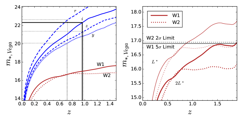
Figure 1.— The apparent magnitude of a passively evolving $L^{\ast}$ galaxy as a function of redshift in various passbands. The plotted curves are for Vega magnitudes and are based upon a Conroy et al. (2009) model with a single $\tau=0.1$ Gyr exponential burst of star formation at $z=3$ and a Chabrier IMF normalized using the $z=1.1$ Spitzer [$3.6$] luminosity function from Mancone et al. (2010). Similar results are obtained for a Bruzual & Charlot (2003) model. Left panel: $m^{*}$ versus $z$ in WISE W1 and W2, and in the four reddest bands provided by Pan-STARRS (Vega magnitudes in all bands). We also plot horizontal lines denoting the Pan-STARRS 50% completeness limits in each band. These are the galaxy completeness limits, which are taken to be 0.4 mag brighter than the point source completeness limits (Metcalfe et al., 2013). The vertical lines indicate the corresponding redshift reach in each filter for the model galaxy. Among the Pan-STARRS passbands, the $i-$band and $z-$band have the greatest redshift reach. For MaDCoWS we use the $i-$band both to provide a greater wavelength lever arm relative to the WISE bands and for consistency with our preliminary SDSS search. The W1 and W2 curves are much flatter with redshift due to negative e+k corrections offsetting the impact of increasing luminosity distance at these wavelengths. Right panel: The horizontal lines show the relevant sensitivity thresholds in W1 and W2 at the median depth of the AllWISE Survey. Galaxies detected at $5\sigma$ in W1 are included in the source catalog; these sources are considered non-detections in W2 if their fluxes fall below a 2$\sigma$ threshold. For comparison we plot the apparent magnitudes of $L^{\ast}$ and 2 $L^{\ast}$ galaxies in the WISE bands. Individual $L^{\ast}$ galaxies at $z\gtrsim 1.1$ are not detected at 5$\sigma$ in W1 for the AllWISE survey depth, but blends of two $L^{\ast}$ galaxies are detectable over the full redshift range shown.

II.2.1 The SDSS Eighth Data Release

The Eighth Data Release of the SDSS (DR8; Aihara et al., 2011) covers $14,555$ deg², mostly in the northern hemisphere, in five optical bands ($ugriz$; Fukugita et al., 1996). The 95% completeness limits in these bands are $u,g,r,i,z=22.0,22.2,22.2,21.3,20.5$ (AB; Abazajian et al., 2009). As discussed below, the most important filter for MaDCoWS is $i$-band, for which the median seeing is $\sim 1.4^{\prime\prime}$.

For the MaDCoWS program, we use data from a more restricted area (hereafter referred to as the WISE—SDSS region). Specifically, we avoid regions at low Galactic latitude ($b<25^{\circ}$), and restrict our use of SDSS data to Galactic cap areas with large, contiguous coverage, avoiding areas with only thin strips of imaging (e.g. see Figure 1 in Aihara et al., 2011). With these restrictions, the remaining SDSS area corresponds to 10,959 deg². After also considering area lost to masking, due to issues such as bright stars and low coverage by WISE, the net effective area in the WISE—SDSS region is 10,290 deg² (see §IV.4).

II.2.2 Pan-STARRS

The Pan-STARRS PS1 3$\pi$ Steradian Sky Survey (Chambers et al., 2016) is designed to provide complete coverage for $\delta>-30^{\circ}$ in $grizy$ with better than 1% photometry in the $grizy$ bands. This data set supercedes SDSS in both area and depth for the MaDCoWS search. There have been three internal releases (processing versions; PV) of stacked $3\pi$ catalogs, plus the Public Data Release DR1 (Flewelling et al., 2016), which corresponds to PV3. For MaDCoWS we are using $i-$band data from the PV2 catalog. This catalog uses the same input image set as PV3/DR1, but differs slightly in how the PSF photometry and star/galaxy flags are implemented. We refer the reader to Laevens et al. (2015) for details on the differences between the different preliminary versions, noting that PV2 is sufficient for the MaDCoWS search since we are only concerned with galaxy photometry in the $i-$band. Most relevant for MaDCoWS, the $i-$band data are $\sim 0.9$ mag deeper than SDSS ($5\sigma$, Metcalfe et al., 2013), yielding lower photometric uncertainties and hence cleaner selection of input galaxies for the cluster search. As with our initial SDSS analysis, with Pan-STARRS we avoid regions at low Galactic latitude. Specifically, we require Galactic latitude $|b|>25^{\circ}$, increasing this limit to $|b|>30^{\circ}$ for Galactic longitude within 60^∘of the Galactic center. These limits correspond to an extragalactic sky area of 23,290 deg², with Pan-STARRS covering 18,120 deg² (78% of the extragalactic sky). After removal of masked regions, areas with low coverage from WISE, and the region near the Galactic plane, the net effective area for the Pan-STARRS search is 17,668 deg², or 76% of the extragalactic sky.

II.2.3 The SuperCOSMOS Sky Survey

While there are multiple ongoing large optical surveys designed to map large areas of the extragalactic sky extending beyond the Pan-STARRS footprint (e.g. Keller et al., 2007; Shanks et al., 2013; Dark Energy Survey Collaboration et al., 2016), no surveys with depth comparable to Pan-STARRS  (or SDSS) yet provide uniformly calibrated catalogs over a large fraction of the sky. At $\delta<-30^{\circ}$ we have therefore undertaken a shallow search using optical data from the SuperCOSMOS Sky Survey (Hambly et al., 2001c, b). The SuperCOSMOS project digitized photographic plates from multiple Schmidt telescopes, initially in the southern hemisphere, with coverage subsequently extended to the entire sky (Hambly et al., 2009). We use SuperCOSMOS data from the UK Schmidt Telescope Red Southern and Equatorial Surveys and the Palomar-II Oschin Schmidt Telescope Red (IIIaF) plates, which are quoted as having nominal depths of $R_{F}\simeq 21.5$ (Vega). From our own testing of the data, we find that it is necessary to restrict our attention to $R_{F}<20.5$ to avoid non-uniformity due to depth variations between plates. Subsequent to our search, Peacock et al. (2016) have constructed an updated all-sky SuperCOSMOS catalog. From the calibration in their analysis, $R_{F}=20.35$ corresponds to a 4$\sigma$ detection; we therefore are using a threshold slightly below 4$\sigma$. The astrometry for this data is accurate to $\pm 0.3^{\prime\prime}$ at this depth (Hambly et al., 2001a), which is sufficient for our program. The total and net effective areas at $\delta<-30^{\circ}$ for the SuperCOSMOS search are 4,260 deg² and 3,828 deg², respectively. Between Pan-STARRS and SuperCOSMOS, we are able to detect clusters across the entire extragalactic sky, with a total combined area of 21,814 deg² after accounting for masking. As discussed in subsequent sections, use of SuperCOSMOS data does yield a significant degradation of the search due to less effective rejection of lower redshift galaxies.

II.3. The Dark Energy Survey

The Dark Energy Survey is in the process of mapping $\sim 5000$ deg² in the region of the southern Galactic cap in the $grizY$ passbands (Abbott et al., 2018). Over half of the DES footprint lies south of $\delta=-30^{\circ}$ and hence outside the Pan-STARRS area, thus providing complementary optical imaging. The photometric depths for the first data release (DES DR1) are $g=24.33$, $r=24.08$, $i=23.44$, $z=22.69$, and $Y=21.44$ (10$\sigma$; Abbott et al., 2018). While the DES DR1 was not availble in time to incorporate into the current MaDCoWS cluster search, we use the $i-$band photometry in §VI.1 to derive photometric redshifts for the subset of cluster candidates that lie within the DES footprint but outside the Pan-STARRS survey area.

II.4. The Spitzer Space Telescope

Our team was awarded Spitzer time during Cycles 9, 11, and 12 to obtain [$3.6$] and [$4.5$] imaging for $1959$ cluster candidates (PI: Gonzalez, PIDs 90177 and 11080), enabling photometric redshift and richness estimates. For the Cycle 9 program, we targeted 200 candidates from a preliminary WISE—SDSS search. In the Cycle 11 – 12 snapshot program we targeted an additional $1759$ clusters, selected by peak amplitude in the WISE—Pan-STARRS and WISE—SuperCOSMOS searches (see §IV.5), that were not previously observed in Cycle 9. We obtain total exposure times of 180 s in each band using a $6\times 30$ s cycling dither pattern. These two programs, both conducted during the Spitzer  “warm” mission, and existing archival data together yield IRAC [$3.6$] and [$4.5$] imaging for $1967$ MaDCoWS clusters. Of these, $1723$ are in the WISE—Pan-STARRS catalog presented in this paper, and $86$ are in the WISE—SuperCOSMOS catalog. The remainder are within the WISE—Pan-STARRS footprint, but are detected at lower significance.

Data were reduced using the MOPEX (Makovoz & Khan, 2005) package and source extraction was performed using SExtractor (Bertin & Arnouts, 1996) in dual image mode with the [$4.5$] image serving as the detection image. During the Spitzer warm mission the FWHM values for the point spread function are 1.95^′′ and 2.02^′′ for [$3.6$] and [$4.5$], respectively, providing a factor of three improvement in spatial resolution relative to WISE. Following the methodology of Wylezalek et al. (2013), we determine that at 10$\mu$Jy the recovered source density in our fields is 95% that of SpUDS at the same threshold. For subsequent analysis we include only sources with $f_{4.5}>10~{}\mu$Jy. We measure our completeness by comparing the MaDCoWS Spitzer number counts with number counts from the Spitzer UKIDSS Ultra Deep Survey (SpUDS, PI: J. Dunlop) survey. The SpUDS survey is a Spitzer Cycle 4 legacy program that observed $\sim$1 deg² in the UKIDSS UDS field with IRAC and the Multiband Imaging Spectrometer (Rieke et al., 2004), reaching $5\sigma$ depths of $\sim 1~{}\mu$Jy at 3.6$\mu$m.

II.5. CARMA

We were awarded time with the Combined Array for Research in Millimeter-wave Astronomy (CARMA) between 2012 and 2014 (PIDs c0884, c1128, c1197, c1272, c1303) to observe a selection of the richest cluster candidates at 31 GHz. We were also awarded time in 2014 September (PID c1272) to target $\sim 150$ cluster candidates with very short exposures to identify very massive clusters. Most of the observations were made with the array in the 23-element CARMA-23 mode, with the exception of the 2012 observations from c0884 and c1128, which used only the eight element SZA. Detections from the pilot run in 2012 and 2013 are presented in Brodwin et al. (2015), and MOO J1142+1527, observed in 2014, is presented in Gonzalez et al. (2015). In the present work, the data were re-reduced using a new version of the SZA MATLAB pipeline (Muchovej et al., 2007) updated to handle 23-element data and produce uv-fits files and the CLIMAX software was used to fit pressure profiles from Arnaud et al. (2010) to the data. The spherically-integrated Comptonization was measured from the Arnaud model, and $M_{500}$, $r_{500}$, and $Y_{500}$ were calculated by forcing consistency with the Andersson et al. (2011) scaling relation. A more detailed description of the observations and analysis is given in Brodwin et al. (2015) and Decker et al. (2018).

III. Cluster Finding with WISE: The Algorithm

III.1. Physical Motivation For Search Algorithm

A number of authors have demonstrated that the stellar mass content of cluster galaxies is tightly correlated with the total cluster mass (e.g. Lin et al., 2004, 2012; Mulroy et al., 2014, and reference therein). Mulroy et al. (2014) for example find an intrinsic scatter of only $\sim 10$% between the $K-$band luminosity and weak lensing mass for nearby clusters. The W1 and W2 WISE bands, which probe approximately rest-frame $H$ and $K_{s}$ at $z\simeq 1$, trace the total stellar mass content, while being relatively insensitive to the age of the stellar population. In the WISE bands the apparent magnitude of an $L^{\ast}$ galaxy is only weakly dependent upon redshift at $z\gtrsim 0.7$ due to e+k corrections that offset the impact of increasing luminosity distance (Figure 1). Consequently, a magnitude-limited galaxy sample selected with WISE has a roughly uniform luminosity limit within this redshift range. Photometry from WISE therefore provides a proxy for stellar mass that is relatively unbiased by star-formation history, and the uniform luminosity limit translates to a uniform selection in stellar mass.

The primary observable for galaxy-based cluster searches is the projected overdensity of galaxies. The luminosity function of cluster galaxies is well-parameterized by the Schechter function (Schechter, 1976), and recent papers have demonstrated that at WISE wavelengths high-redshift galaxy clusters have relatively flat faint end slopes (e.g. Mancone et al., 2012). Combined with the rising number counts of the field population at faint magnitudes, a cluster will have the greatest density contrast relative to the background population when the limiting magnitude of the input galaxy catalog is slightly below $L^{\ast}$. Thus, while W2 offers the more uniform stellar mass limit with redshift, for MaDCoWS we use a W1$-$selected galaxy sample due to the greater depth relative to $L^{\ast}$ in this band. For $z\simeq 1$ the W1 AllWISE imaging reaches 1.1$L^{\ast}$ at 5$\sigma$, while the [4.6] imaging only reaches approximately 2.1$L^{\ast}$ at 5$\sigma$ ($M^{\ast}$$-0.8$), or 0.85$L^{\ast}$ at 2$\sigma$ ($M^{\ast}$$+0.2$; Figure 1). With MaDCoWS  we are therefore effectively searching for $z\sim 1$ galaxy clusters via overdensities of galaxies with luminosities of approximately $L^{\ast}$ or greater.

In practice, one additional consideration that impacts the effective depth is source blending in WISE due to the large PSF. Blending affects the number of observed galaxies in two competing ways. First, blending decreases the number of individual detections for galaxies brighter than the apparent magnitude limit. Second, blending leads to detections arising from blends of galaxies that are individually fainter than the detection limit. For the general field population the net impact of these two factors will be a uniform shift in the number counts as a function of magnitude, which does not impact our cluster search. For clusters, both factors will have the greatest effect in the core region where the projected density is highest. For MaDCoWS, because the magnitude limit is close to $L^{\ast}$, the second effect will generally dominate due to the higher surface density of galaxies with $L<$$L^{\ast}$ compared to super-$L^{\ast}$ galaxies. The MaDCoWS search therefore ends up benefitting from inclusion of blended galaxies that are individually somewhat fainter than the nominal WISE detection limit. For illustration, we show WISE and Spitzer imaging for one of the spectroscopically confirmed MaDCoWS clusters in Figure 2.

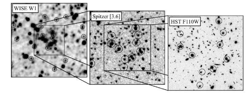
Figure 2.— Progressively zoomed images for the cluster MOO J1514+1346 ($z=1.059$, Brodwin et al., 2015). The left panel is a $5^{\prime}\times 5^{\prime}$ W1 image from the AllWISE survey, while the middle panel is a deeper Spitzer [$3.6$] image from our Cycle 9 program of the central $2^{\prime}$ region. In the right panel we show an HST F110W image of the central $75^{\prime\prime}$ (555 s exposure; Program 14456, PI: Brodwin), with black circles indicating the locations of the objects from the WISE catalog that contributed to detection of the cluster. The diameter of each circle is $6.1^{\prime\prime}$ in the Spitzer and HST images, equivalent to the FWHM of the WISE W1 PSF. For the WISE image we use a larger 9^′′ circle for clarity. This sequence of images illustrates the impact of blending upon detection. While bright cluster galaxies are the main source of signal for cluster detection, unresolved blends of cluster galaxies also contribute to cluster detection.

III.2. Algorithm Details

The concept for the MaDCoWS algorithm, though different in detail, is in the spirit of previous cluster searches using Spitzer data. The basic idea is to first isolate the distant galaxy population, using color and magnitude cuts to minimize foreground contamination, and then use wavelet filtering to identify the most significant overdensities on cluster scales. The color and magnitude selections, as described below, are similar to those employed by Papovich (2008) and Muzzin et al. (2013), while the wavelet technique draws upon the legacy of the ISCS and IDCS (Eisenhardt et al., 2008; Stanford et al., 2012).

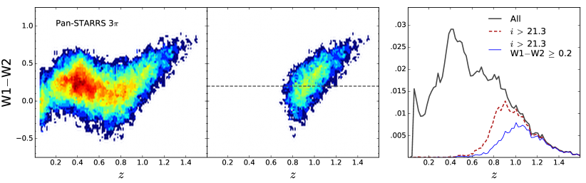
Figure 3.— Illustration of the impact of the color and magnitude cuts using a sample of WISE sources matched to the photometric redshift catalog for IRAC-selected sources in the NDWFS region (Brodwin et al., 2006). Left: Density map of the WISE color distribution as a function of photometric redshift for all galaxies with W1$<16.9$. Center: Density map showing the redshift distribution of galaxies from the left panel with $i>21.3$. The optical magnitude cut, based upon Pan-STARRS photometry, effectively removes foreground galaxies at $z<0.8$. The dashed line shows the WISE color cut. Use of SDSS rather than Pan-STARRS photometry in the initial search yields a nearly identical selection. Right: The redshift distribution of the full galaxy sample from the left panel (black), galaxies with $i>21.3$ (red), and those passing both the optical magnitude and WISE color cuts (blue). The addition of the W1$-$W2 color cut increases the mean redshift of the remaining galaxy population, but has minimal impact on foreground removal.

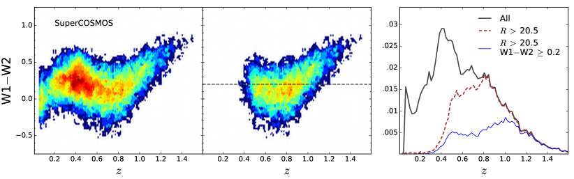
Figure 4.— The panels in this figure are the same as in Fig. 3, but now using SuperCOSMOS photometry for optical rejection. this figure illustrates that the optical magnitude and WISE color cuts are less effective for the shallower SuperCOSMOS catalog, resulting in a significantly higher fraction of low-redshift interloper galaxies.

III.2.1 Galaxy Selection

For the MaDCoWS cluster search, we start with the full WISE catalog of all sources detected at 5$\sigma$ in W1. We then impose a magnitude cut W1$<$16.9 to enforce uniformity of depth for the galaxy catalog.

The optical magnitude criterion is applied next. Within the Pan-STARRS region we reject sources with $i<21.3$ ($i<20.93$ Vega). In Figure 3 we cross-match WISE sources within the NOAO Deep Wide-Field (NDWFS) region with a photometric redshift catalog for IRAC-selected sources from Brodwin et al. (2006) to illustrate the impact of our cuts. As can been seen in this Figure, the optical rejection effectively removes galaxies at $z\lesssim 0.8$. In Figure 3 we also show the redshift distribution in the WISE bands of all sources surviving this cut. The $i-$band magnitude of this cut is predominantly empirical based upon the data shown in Figure 3, but set at a physical level where no cluster galaxies, except potentially BCGs at $z\simeq 0.8$ are removed. For the same evolutionary model as in Figure 1, this magnitude limit corresponds to a 1.8 $L^{\ast}$ galaxy at $z=0.8$. Use of a brighter magnitude cut increases foreground contamination, while using a significantly fainter cut would diminish the cluster signal. Outside the Pan-STARRS region we reject sources with $R_{F}<20.5$ from SuperCOSMOS, a shallower cut that is less effective at removing low-redshift interloper galaxies. In Figure 4, we illustrate the approximate impact of this cut by applying an $R>20.5$ cut within NDWFS. These interlopers decrease the density contrast between clusters and the field – and hence larger scatter between detection amplitude and richness, and also result in higher contamination of the sample by low-redshift clusters (see §VI.2).

Subsequent to the optical cut, we impose a WISE color cut, rejecting objects with W1$-$W2$<0.2$. As a precaution at this stage we also reject galaxies not detected at 2$\sigma$ in W2. The WISE color cut preferentially removes galaxies at $z<0.8$ from the galaxy population remaining after the optical rejection. For the WISE—Pan-STARRS region, the median redshift increases from 0.93 to 1.01 with the addition of the WISE color cut (see the redshift distributions in the rightmost panel of Figure 3). As a result, clusters at $z\lesssim 1$ are downweighted in the WISE–Pan-STARRS search. Outside the Pan-STARRS region, because of the shallower SuperCOSMOS optical cut, this color cut is vital for reducing contamination from galaxies at $0.5\lesssim z\lesssim 0.8$. This can be seen in the center and right panels of Figure 4. It is worth emphasizing that even with the WISE color cut, the lack of SDSS- or Pan-STARRS-quality optical data has a detrimental impact on the search at $\delta<-30^{\circ}$. We discuss in §VI.6 prospects for an improved southern search.

III.2.2 Identifying Galaxy Overdensities

From the filtered galaxy catalogs, we construct density maps with a resolution of 15^′′. These density maps are filtered with a Difference-of-Gaussians kernel (similar to a Mexican hat kernel) to identify cluster-scale overdensities. The functional form for this kernel is

$$K=\frac{1}{2\pi\sigma_{1}^{2}\sigma_{2}^{2}}\left(\sigma_{2}^{2}\exp(-\frac{r^{2}}{2\sigma_{1}^{2}})-\sigma_{1}^{2}\exp(-\frac{r^{2}}{2\sigma_{2}^{2}})\right),$$ (1)

where $\sigma_{1}$ and $\sigma_{2}$ are the scales of the inner and outer Gaussians, respectively. This kernel functions as a bandpass filter (much like the filters in the SZ surveys), removing contributions to the density map from large scale structure and other sources of gradients in the projected galaxy density on large scales. The form of the kernel is shown in Figure 5. Details regarding the specific scales set for the kernel are presented in §IV.4.

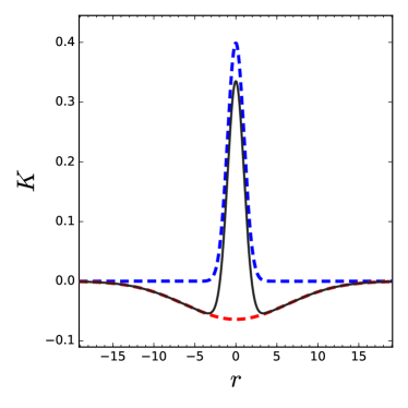
Figure 5.— A cross-sectional representation of a normalized, two-dimensional Difference-of-Gaussians kernel (black, solid curve). For illustration, we plot a kernel with $\sigma_{1}=1$ and a 2.5:1 scale ratio. The two dashed curves show the inner (blue) and outer (red) Gaussians used to construct the kernel. This kernel acts as a bandpass filter. Structures on scales smaller than the inner kernel are smoothed out, while those on scales larger than the outer component are effectively removed as a background component.

IV. Cluster Finding with WISE: Implementation

IV.1. Catalog Cleaning

Both the WISE and optical catalogs contain quality flags for each source. For WISE, the catalog contains information on sources that are flagged as contaminants in cc_flags, which can arise from optical ghosts, diffraction spikes, persistence effects, or scattered light. We reject sources with cc_flags$\neq 0$ in W1 or W2, as non-zero flags are indicative that the source detection may be unreliable or measurements for that source may be contaminated. We also reject sources that are flagged as optical ghosts in either W3 or W4 as a precaution. While we are not using W3 and W4 photometry, the detection of an optical ghost in these bands is indicative of potential contamination from ghosts at shorter wavelengths – which may not always be flagged.

The above criteria are designed to maximize the purity of the WISE catalog, and hence minimize spurious cluster detections. For the optical catalogs, the more important factor is completeness because the optical photometry is used to reject low-redshift interlopers. Put simply, it is better to be able to use the existence of an optically bright source with some quality issues to identify a WISE source as low-redshift than to allow that interloper to contribute to the density map. We therefore minimize the rejection due to flagging in the optical catalogs to the extent possible. For the SDSS catalog, we require that all sources are primary for the initial SQL query when downloading the data from CASJobs, but apply no additional filters. For Pan-STARRS  we apply no filters to the source catalog. For SuperCOSMOS we reject sources for which the $R_{F}$-band quality flag indicates a severe defect.

IV.2. Matching WISE and Optical Catalogs

To match the optical and WISE catalogs, we perform a nearest neighbor match for each WISE detection. We consider a match to be a true physical association if the separation is less than 1.5^′′ from each WISE detection. This matching radius was set empirically to be sufficiently large to robustly identify true matches, while minimizing the rate of spurious associations. In Figure 6 we show the distribution of nearest neighbor matches for WISE sources. For associations within $3^{\prime\prime}$, 90% of matches have separations less than our 1.5^′′ threshold. The AllWISE Explanatory Supplement (section II.5.b) quantifies the distribution of astrometric offsets between WISE and UCAC4 (Zacharias et al., 2013), accounting for proper motions, finding a standard deviation $\sigma\simeq 0.55^{\prime\prime}$ at W1$=$16. Our matching radius is thus slightly less than the 3$\sigma$ astrometric uncertainty.

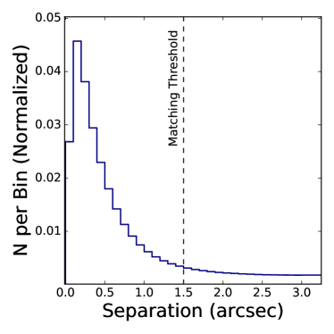
Figure 6.— The distribution of separations between WISE sources and the nearest Pan-STARRS source. The vertical dashed line shows the 1.5^′′ search radius used to match WISE and Pan-STARRS sources in the MaDCoWS cluster search.This matching radius is selected to be large enough to robustly associate true physical WISE—Pan-STARRS matches, while minimizing the rate of spurious associations.

IV.3. Tiling the Sky

Once the WISE and optical catalogs have been cross-matched, we apply the magnitude and color cuts described in §III.2.1 and construct density maps from the remaining sources. For existing Spitzer searches for high-redshift galaxy clusters, which typically cover $<100$ deg², there is generally no need to subdivide the survey region. In contrast, for MaDCoWS it is necessary to develop a tiling strategy to subdivide the search region, enabling efficient handling of the catalogs and generation of density maps. The chosen approach is to conduct the search within $10^{\circ}\times 10^{\circ}$ tiles, each of which overlaps with neighboring tiles by approximately 1^∘. The overlap regions are used for validation in assessing the robustness of the search results.

IV.4. Constructing the Density Maps

For each tile we generate a raw density map with a resolution of 15^′′ pix^-1. Each galaxy that passes the color, magnitude, and quality cuts described above is then inserted into the raw density map, using a smoothing kernel that assigns uniform weight over a width of two pixels. The result is a number-weighted projected galaxy density map. We note that one could instead attempt to use a flux-weighted map given the weak dependence of W1 upon redshift at $z\gtrsim 0.7$ (Figure 1). Such a flux-weighted approach has the advantage of giving greater weighting to blended galaxies in cluster cores that are undercounted in number-weighted maps; however, flux-weighted maps also amplify the impact of bright contamination from low-redshift interlopers. Moreover, increasing the importance of individual bright cluster galaxies for cluster detection is not necessarily desirable, as detection becomes more sensitive to omission of a single galaxy from the density map due to the photometric quality cuts.

An important element of generating the density maps is construction of corresponding masks to properly account for survey boundaries, regions around bright stars, and low coverage regions. For masking we use a two stage approach. First, we generate masks directly from the WISE catalog data in parallel with construction of the density maps. For every source that passes the quality cuts, the value for the coverage at that location is used as input to generate an initial coverage map at the same resolution as the density map. A smoothing kernel is applied to the map to interpolate the coverage map over pixels lacking sources. These smoothed coverage maps are then converted into binary masks associated with each raw density map, effectively masking regions of low coverage. For coverage, we define a location as having low coverage if there are fewer than 20 single frame exposures in either W1 or W2. For reference the standard two epoch coverage from AllWISE corresponds to twenty-two observations (Cutri et al., 2013). In practice, our low coverage restriction has little impact upon the MaDCoWS survey because the AllWISE coverage in our survey region rarely falls below 20 exposures (see Figure 7 in section IV.2. of the AllWISE Explanatory Supplement (Cutri et al., 2013). At this stage we also mask regions that lie outside the footprint of the associated optical data set.

Second, we use the WISE source catalog to mask regions near bright stars. Within the region of the scattered-light halo for bright stars, the photometry for fainter objects can be contaminated. It is therefore best to avoid these sources in the survey. Table 11 in section 4.4.g.ii.1.a of the All-Sky Explanatory Supplement provides coefficients relating the halo radius for scattered light halos to the magnitude of the source. Using this relation, we mask all sources with halo radii larger than 1^′ (W1$<6.8$) out to the halo radius.

Once the raw density map and mask are generated, we next convolve both with the Difference-of-Gaussians kernel (Equation 1). For the inner and outer Gaussians, we use a 6:1 ratio of outer to inner radii, setting $\sigma_{1}=38.2^{\prime\prime}$ and $\sigma_{2}=3.82^{\prime}$ (320 kpc and 1.9 Mpc at $z=1$, respectively). The value of $\sigma_{1}$ is similar to that used for the ISCS and IDCS surveys (400 kpc and 300 kpc, respectively), while for MaDCoWS $\sigma_{2}$ is larger than for those surveys (1.6 Mpc and 1.2 Mpc, respectively). Physically, the larger $\sigma_{2}$ is designed to avoid oversubtraction for the most massive clusters, for which the signal can extend to larger radii. Dividing the convolved density map by the convolved mask properly removes gradients in the smoothed images that arise from the masking.

IV.5. Extracting Cluster Detections

Within the smoothed density maps, we use Source Extractor (Bertin & Arnouts, 1996) to identify candidate clusters. Source Extractor is run on each tile with no background subtraction. Only a single pixel is required to exceed the detection threshold for a source to be selected. Specifically, we define the peak amplitude for a source to be the maximum pixel value associated with a detection in the smoothed density maps (which is equivalent to FLUX_MAX in SExtractor), and only this peak amplitude must exceed the threshold for a source to be detected. Detections from all tiles are then combined to form a single catalog; within overlap regions detections are merged to eliminate duplicates. For all cluster candidates we also calculate signal-to-noise based upon the peak amplitude and the RMS noise in the tile within which a cluster is detected.

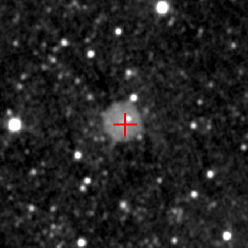
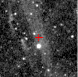
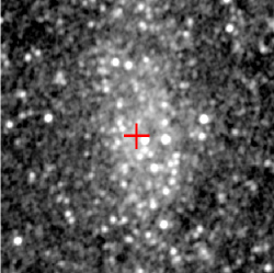
Figure 7.— W2 images ($10^{\prime}\times 10^{\prime}$) showing examples of contamination that is removed by visual inspection. In each panel the cross denotes the location of the detection. The left, center, and right panels respectively correspond to spurious detections caused by an optical ghost, scattered light, and a nearby dwarf galaxy. In the latter case, the galaxy is Wolf-Lundmark-Melotte (DDO 221; Wolf, 1909) at a distance of 933 kpc (McConnachie, 2012).

From the remaining candidate list, we then search through the 2MASS Extended Source Catalog (Jarrett et al., 2000) and remove all candidates that lie within twice the total magnitude extrapolation radii (r_ext) of the 2MASS extended sources. This cut, which is designed to remove peaks that may be associated with substructure in nearby galaxies, eliminates 8% of candidates. We next impose the Galactic latitude restrictions mentioned in §II. We restrict our search to $|b|>25^{\circ}$ for the WISE—Pan-STARRS and WISE—SDSS data sets, increasing the Galactic zone of avoidance to $|b|>30^{\circ}$ for cluster candidates at $300^{\circ}<l<360^{\circ}$ and $0^{\circ}<l<60^{\circ}$. For the WISE—SuperCOSMOS search we opt to maintain a $|b|>30^{\circ}$ Galactic zone of avoidance at all $l$. For the SuperCOSMOS search we also apply avoidance regions near the Magellanic Clouds. We impose the restriction that candidates cannot lie within $3^{\circ}$ of the SMC, or within an ellipse with semi-major axes of $13^{\circ}$ and $4.5^{\circ}$ for the LMC. In practice, this exclusion cut did not remove any candidates from the catalog presented below.

At this stage we also apply an automated rejection of all cluster candidates for which the peak flux lies in a pixel adjacent to a masked region (12% of detections). While the majority of these sources are expected to be true clusters, these sources have an enhanced likelihood of being spurious due to contamination near diffraction spikes of bright stars or other subtle image artifacts. Moreover, the peak fluxes for clusters on mask edges will often be underestimated due to the masking. For these reasons we opt for a modest sacrifice in area for increased catalog fidelity and uniformity.

Finally, our team visually inspects WISE cutouts of each candidate in W1 and W2 to identify any non-cluster sources of peaks in the wavelet maps. There are three main sources of such contamination, examples of which are shown in Figure 7. The first source is optical ghosts, which for WISE appear as ring-like structures at a fixed position from the parent star. While optical ghosts are flagged as artifacts during generation of the WISE catalog, we have found that there exist some instances where these sources are not flagged, resulting in clusters of sources that in catalog space mimic a cluster detection. Additional examples of WISE optical ghosts can be see in Figures 19–21 of section II.4.b.ii of the All Sky Explanatory Supplement. The second source of contamination arises from scattered light. Scattered light can yield anomalously red sources, and can induce spurious sources of a common color in the images. The third main source of contamination consists of local galaxies not present in the 2MASS Extended Source catalog. All the above sources of contamination are easily identifiable visually. In addition to these three main contributors, we also remove a small number of detections associated with satellite trails and other rare anomalies. In total, visual inspection removes 6% of the candidates which remain after automated rejection.

V. The Catalog

We describe in this section the properties of the ensemble of cluster candidates that remain after the detection and cleaning stages. For both the WISE—Pan-STARRS  and WISE—SuperCOSMOS searches we present catalogs of all sources detected above thresholds in peak amplitude (see V.2). The precise detection thresholds are set such that a cluster with a peak amplitude exceeding this threshold would have SNR$\geq 8$ in any survey tile. The motivation for this specific SNR criteria is simply that it yields a sample for which most of the WISE—Pan-STARRS clusters have Spitzer photometry. For WISE—Pan-STARRS, the catalog includes $2433$ clusters, which are presented in Table LABEL:tab:panstarrsclusters. For the WISE—SuperCOSMOS search the noise levels are higher due to the shallower optical data, and the catalog is correspondingly smaller. We present the $250$ clusters in this region in Table 4. We also publish data for all clusters from our earlier WISE—SDSS search for which we have Spitzer imaging, but which are not detected above the threshold of the WISE—Pan-STARRS catalog. A key contributing factor in their omission from the WISE—Pan-STARRS catalog is that subsequent to the preliminary WISE—SDSS search increased masking was employed and the color cuts were tweaked, which together led to these clusters being either masked or detected below the peak amplitude threshold. Spectroscopic redshifts, masses, and cross-identifications are provided in the comments when applicable. The designation for MaDCoWS candidates in all tables is MOO, which stands for Massive Overdense Object. In Table LABEL:tab:panstarrsclusters we include photometric redshifts and richnesses (as defined in §VI.1 and VI.3, respectively) for the $1723$ clusters with Spitzer imaging. Similarly, in Table 4 we include photometric redshifts and richnesses for 64 clusters from the WISE—SuperCOSMOS search with Spitzer imaging that lie within the DES footprint. In Table 1 we summarize the total number of clusters and number of clusters with IRAC photometry for each of these catalogs.

Table 1Summary of Catalog Sample Sizes

	Clusters	IRAC Subsample
WISE—Pan-STARRS	$2433$	$1723$
WISE—SuperCOSMOS	$250$	$86$
WISE—SDSS	$156$	$156$

V.1. Spatial Distribution

Because of the Difference-of-Gaussians filtering, the MaDCoWS cluster search is relatively insensitive to larger scale variations in the source counts, which can arise from a variety of observational (sensitivity gradients) and astrophysical (foreground extinction, large scale structure) effects. In Figure 8, we show the projected distribution of the $2433$ highest amplitude detections in the WISE—Pan-STARRS region and the $250$ highest amplitude detections over the rest of the extragalactic sky. The effective area of the WISE—Pan-STARRS region after accounting for masking (17,668 deg²) constitutes 82% of the combined area covered by the WISE—Pan-STARRS and WISE—SuperCOSMOS searches. As discussed in §IV.5, we avoid $|b|\leq 25^{\circ}$ over the full sky, and widen our Galactic zone of avoidance both for the SuperCOSMOS search and towards the Galactic center.

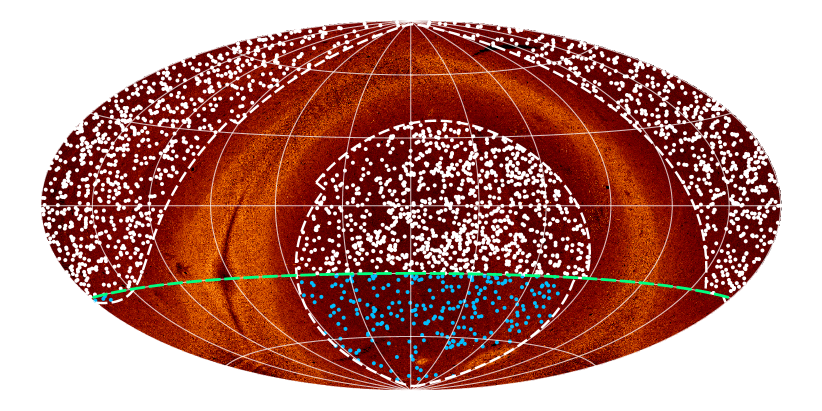
Figure 8.— Distributions of cluster candidates from the WISE—Pan-STARRS and WISE—SuperCOSMOS searches atop a WISE source density map. White circles denote the $2433$ candidates from the WISE—Pan-STARRS region that are presented in Table LABEL:tab:panstarrsclusters, while blue circles identify the $250$ highest amplitude candidates found outside this region using WISE and SuperCOSMOS data (see Table 4). The white dashed curves delineate the Galactic zone of avoidance, which lies at $|b|<25^{\circ}$ for the Pan-STARRS region more than 30^∘ in longitude from the Galactic center, and at $|b|<30^{\circ}$ near the Galactic center and within the SuperCOSMOS region. The green curve at $\delta=-30^{\circ}$ corresponds to the southern limit of the Pan-STARRS survey.

V.2. Peak Amplitudes

The measured peak amplitude of an overdensity in the smoothed maps, as defined in section IV.5, is the observable quantity used to select clusters for the MaDCoWS catalog. The distribution of peak amplitudes for the WISE—Pan-STARRS search, normalized such that the most significant peak has an amplitude of 1, is shown in Figure 9. It is approximately a power law in number versus peak amplitude. For a given detection, the amplitude of a peak is determined by the number of galaxies associated with the cluster core and the physical size of the smoothing kernel.

While this quantity provides the best direct observable for identifying clusters in the MaDCoWS search, it is important to understand that peak amplitude is only a coarse tracer of the true cluster richness. We therefore expect broad dispersions in cluster richness and mass for a given observed peak amplitude. There are several reasons for this scatter. First, the number of galaxies contributing to a given overdensity in the smoothed maps will be dependent on the redshift of the cluster (due to both the optical magnitude and WISE color cuts, which have the greatest impact at lower redshifts, and the fixed limiting apparent magnitude). Second, the observed number of galaxies is affected by blending in the WISE data, which will be most pronounced for the richest and most centrally concentrated clusters. Third, the observed peak amplitude will also be affected by physically associated structures along the line of sight such as filaments. The net impact of this scatter is that for a catalog selected at a fixed peak amplitude threshold, the completeness at a fixed mass threshold is expected to be relatively low – put succinctly, we detect massive clusters, but not in a statistically complete sense as would be needed for derivation of cosmological constraints.

Keeping this limitation in mind, as an initial validation of our approach we use IRAC photometry to confirm that the WISE candidates selected via peak amplitude correspond to overdensities of red galaxies. We directly counted the number of red galaxies (defined as [$3.6$]$-$[$4.5$]$>0.1$ Vega) within 1^′ of the cluster centroid defined by the IRAC data (see §V.3) for the $1723$ clusters from the Pan-STARRS region with IRAC photometry. For comparison, we applied the same criteria to derive the equivalent density of red galaxies for 50 massive clusters from the South Pole Telescope ($0.9<z_{phot}<1.3$) and for a distribution of random locations from the Spitzer Public Legacy Survey of the UKIDSS Ultra Deep Survey (SpUDS; Kim et al., 2011). We show the results of this comparison in Figure 10. By this IRAC-based measure, both the SPT-SZ and MaDCoWS clusters have distributions with significantly higher median values of $N_{gal,1^{\prime}}$ (43 and 44, respectively) than the random field locations from SpUDS (6.6). This Figure indicates that MaDCoWS is identifying true overdensities, but should be taken only as illustrative. In §VI.3 we derive a higher-fidelity richness estimator incorporating background subtraction, and we revisit the topic of the mass distribution of MaDCoWS clusters in §VI.4.

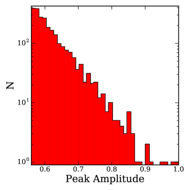
Figure 9.— Histogram showing the distribution of the peak amplitudes for detections in the Pan-STARRS catalog, normalized so that the highest amplitude detection has an amplitude of 1.

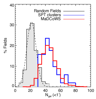
Figure 10.— Comparison of IRAC richnesses, defined as the number of galaxies with red IRAC colors that lie within a 1^′ circle of the cluster locations, for MaDCoWS cluster candidates (red) with $z>0.9$ SPT-SZ clusters (blue), and with random locations in the SpUDS field survey (shaded grey, with the dashed black line denoting a best fit Gaussian). The MaDCoWS cluster candidates and SPT-SZ clusters on average have similar overdensities of red galaxies, with both samples significantly exceeding the random field distribution.

V.3. Astrometric Precision

There are two factors that limit the astrometric precision of the locations presented for the cluster candidates. The first is the resolution of the smoothed density maps. The coordinates presented correspond to the central value for the pixel with the peak flux associated with each detection, with no sub-pixel interpolation. The precision of these coordinates is therefore limited by the 15^′′ pixel scale of the density maps. Second, the shot noise associated with each detection is significant, given that the detections are typically based upon only the $L\gtrsim$$L^{\ast}$ galaxy population in the presence of both source confusion and foreground and background contamination. To quantitatively estimate the centering uncertainty associated with these positions, we use the IRAC photometry to calculate the centroid of the galaxy distribution as defined by the deeper Spitzer data for the subset of galaxy clusters in the WISE–Pan-STARRS catalog with existing IRAC imaging.

Details of the Spitzer centroiding will be described in an upcoming paper focused upon the Spitzer catalogs; most pertinent for the current discussion is that the centroids are number-weighted and defined using galaxies detected at 3.6$\mu$m down to the completeness limit of 10 $\mu$Jy, which corresponds to roughly a 0.3 $L^{\ast}$ galaxy at $z=1$ (Mancone et al., 2010). Centroids correspond to the most significant density peaks of galaxies within 1^′ of the MaDCoWS location. This matching radius corresponds to 500 kpc at $z=1$, and is set to be substantially larger than the expected centroiding error. For this centering comparison we apply no [$3.6$]$-$[$4.5$] color cut to the IRAC photometry. This choice maximizes the signal for centroiding and avoids spurious centroids for any low-redshift clusters in the sample. We include in Table LABEL:tab:panstarrsclusters both the original detection coordinates and the Spitzer-derived centroids.

In Figure 11 we show the distribution of offsets. The average catalog and centroid coordinates are co-centric to within 1^′′, with standard deviations $\sigma_{\alpha}=14.3^{\prime\prime}$ and $\sigma_{\delta}=15^{\prime\prime}$ ($\sim 1$ pixel). For clusters at $z=1$, the two-dimensional positional uncertainty of 21^′′ corresponds to a physical uncertainty of 175 kpc in the cluster position relative to the peak of the galaxy density distribution derived from Spitzer data.

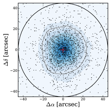
Figure 11.— Distribution of offsets between the cluster positions from the MaDCoWS search and the centroid of the galaxy distribution defined with Spitzer. For centroids within 45^′′ (91%), which we take as the maximum separation for real matches (black circle), the rms scatter is $14.3^{\prime\prime}$ in Right Ascension and $15^{\prime\prime}$ in Declination, nearly identical to the 15^′′ pixel scale used in the cluster search. The red cross denotes zero offset. The shading corresponds to a smoothed density map generated using kernel density estimation, while the grey contour encloses 68.3% of the clusters.

VI. Survey Characterization

In the previous section we presented the MaDCoWS catalog and basic properties of the cluster candidates. We now proceed with a more extended discussion of derived properties of the candidates and sample based upon additional data obtained for subsets of the sample.

VI.1. Photometric Redshift Calibration

We have previously reported spectroscopic redshifts for MaDCoWS clusters in Gettings et al. (2012), Stanford et al. (2014), Brodwin et al. (2015), Gonzalez et al. (2015), and Decker et al. (2018). In this paper we provide spectroscopic confirmation for one additional cluster, MOO J1229+6521, which also appears in the Planck cluster catalog as PSZ2 G126.57+5161 (Planck Collaboration et al., 2016b). Observational details and individual redshifts for newly confirmed members of this cluster are reported in Appendix B. Literature redshifts also exist for several known clusters (Hilton et al., 2007, 2018). The full spectroscopic sample includes 39; the subset of 38 clusters which have both spectroscopic data and IRAC photometry serves as the validation set for our photometric redshifts.

We derive photometric redshifts based upon the [$3.6$]$-$[$4.5$] colors of cluster galaxies, augmented by $i-$[$3.6$] color information. This approach is similar to that of Muzzin et al. (2013), who used a combination of $z-$band and IRAC photometry to derive photometric redshifts. Figure 12 shows $i-$[$3.6$] versus [$3.6$]$-$[$4.5$] color of galaxies in the field of one of our spectroscopically-confirmed clusters, MOO J1142+1527 ($z=1.189$). Also shown is a curve tracing the expected colors as a function of redshift for a passively evolving galaxy with solar metallicity formed via a single stellar burst at $z_{f}=3$, using EzGal (Mancone et al., 2012, www.baryons.org/ezgal) and the Flexible Stellar Population Synthesis code (FSPS, Conroy et al., 2009; Conroy & Gunn, 2010).

To compute the effective color of the ensemble of cluster galaxies, we first select all galaxies with $f_{4.5}>15\mu$Jy that lie within $1^{\prime}$ of the cluster centroid. We then construct a smoothed density distribution using a kernel density estimation algorithm. The peak of this smoothed density distribution is taken as the representative color of cluster galaxies. For the subset of candidates with multiple color peaks, we associate the brightest peak with the cluster but also calculate the colors of any secondary or tertiary peaks. We report the redshifts of these peaks only if the derived richnesses (see §VI.3) exceed that of the primary peak. In principle, the peak of the smoothed density distribution associated with the cluster should lie close to the model curve for passive cluster populations, and blueward of the curve in $i-$[$3.6$] for star-forming galaxies. In practice, the $i-$[$3.6$] peak color is not well-constrained because many cluster galaxies are non-detections in Pan-STARRS. Inclusion of galaxies with only magnitude limits in $i-$band results in the peak of the distribution being biased towards bluer $i-$[$3.6$].

To infer redshifts from the color distribution, we rely primarily on the more robust [$3.6$]$-$[$4.5$] color. This color increases monotonically at $0.7<z<1.7$, and within this redshift range we calculate the photometric redshift by determining the model redshift which yields the [$3.6$]$-$[$4.5$] color closest to that of the peak of the smoothed density distribution. While the IRAC photometry alone is sufficient to derive low-scatter photometric redshifts for clusters at $z>0.7$, the expected [$3.6$]$-$[$4.5$] colors of cluster galaxies at $0.7<z<1.15$ are degenerate with those of galaxies at $z<0.7$. We use the $i-$[$3.6$] color to break this degeneracy. For low-redshift structures the galaxies are brighter and the $i-$[$3.6$] colors bluer, yielding detections rather than upper limits, and enabling robust determination of the low-redshift solution.

The strongest peaks in the smoothed density maps correspond to $z<0.7$ for $\sim 2$% of the full ensemble of candidates with Spitzer/IRAC photometry. Using data from the Legacy Surveys (Dey et al., 2018) we visually inspected the subset of these 2% that lie within the Dark Energy Camera Legacy Survey DR7 footprint. In all cases, we find that the low-redshift peak in color space is a foreground cluster unassociated with the galaxies that contributed to the MaDCoWS detection. For this reason, we impose a prior on the photometric redshift estimates, requiring that the solution lie at $z\geq 0.6$ for the WISE—Pan-STARRS and WISE—SDSS catalogs. In cases where there is a strong peak in the color distribution corresponding to a low redshift cluster, we note in the Tables the presence of a foreground structure. There are total of six clusters in the two catalogs (0.3% of the Spitzer sample) for which it is not possible to recover a redshift and richness for the background cluster. In these cases we simply note the presence of the foreground structure. For the WISE—SuperCOSMOS catalog, which lies outside the DR7 footprint and has less robust removal of foreground galaxies (see Fig. 4), we impose no prior.

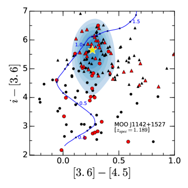
Figure 12.— Color-color diagram for MOO J1142+1527 ($z=1.189$; $M_{500}=5.7\pm 0.5\times 10^{14}$ M_⊙). All magnitudes are Vega. Only galaxies with $f_{4.5}>15~{}\mu$Jy that lie within 2^′ ($\sim 1$ Mpc) of the cluster center are shown. Circles denote galaxies detected in all bands; triangles indicate galaxies with lower limits in $i-$[$3.6$]. Red symbols indicate galaxies that lie within 1^′ of the cluster centroid. The light blue color map indicates the smoothed density distribution derived from the red points. The lowest density threshold corresponds to 40% of the maximum height of the smoothed distribution, with color intervals spaces by 10%. The dark blue curve shows the model track from $z=0-1.7$ for a passively evolving galaxy formed at $z=3$. The yellow star indicates the peak of the density distribution, which is used to determine the photometric redshift, $z_{phot}=1.10^{+0.05}_{-0.04}$. We note that the derived density distribution and yellow star are biased towards bluer $i-[3.6]$ color due to the inclusion of lower limits on $i-[3.6]$ when computing this distribution. This offset will be generally be true for MaDCoWS clusters at $z\sim 1$, for which the $i-$band data are only providing lower limits on the colors of cluster galaxies. It does not however yield a corresponding bias in the photometric redshifts because [$3.6$]$-$[$4.5$] increases monotonically at $z\gtrsim 0.7$.

Comparing with the 38 spectroscopic redshifts (Figure 13), we find two outliers for which the photometric redshifts are $>5\sigma$ from the spectroscopic redshift. For the rest of the sample the scatter is $\sigma_{z}/(1+z)=$0.036. For all clusters with Spitzer/IRAC photometry, which is essential for achieving this fidelity in the redshift estimates, we include in Table LABEL:tab:panstarrsclusters the photometric redshifts and associated uncertainties.

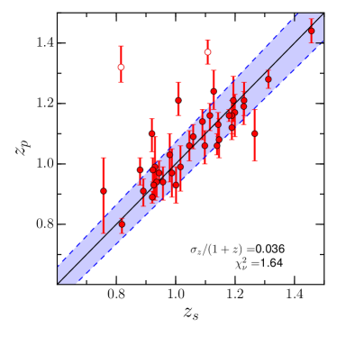
Figure 13.— Comparison of photometric and spectroscopic redshifts for confirmed MaDCoWS clusters. The solid line is the one-to-one relation, while the shaded region corresponds to the interval $\sigma_{z}/(1+z)=0.036$. The points denoted as open circles are the two clusters for which the photometric redshifts are $>5\sigma$ outliers.

VI.2. Redshift Distribution

In Figure 14 we show the photometric redshift distribution for MaDCoWS cluster candidates within the Pan-STARRS region with Spitzer photometry (blue solid curve). We also show the redshift distribution for all MaDCoWS clusters within the Pan-STARRS region with spectroscopic redshifts (red dashed). The curves shown are derived using Gaussian kernel density estimation, applying Scott’s rule (Scott, 1992) to calculate the estimator bandwidth. The general similarity of the curves illustrates the robustness of the estimated redshift distribution. The low-redshift cutoff seen in the full sample arises primarily from the magnitude and color cuts used in the initial galaxy selection for the cluster search, while the high-redshift decline is due to a combination of a decrease in the number density of massive clusters and the W1 band not quite reaching constant stellar mass with increasing redshift.

In Figure 14 we also plot the photometric redshift distribution for MaDCoWS clusters within the SuperCOSMOS footprint with Spitzer photometry (green dot-dashed). As expected, the redshift distribution is shifted to slightly lower redshift relative to the Pan-STARRS sample, with median redshifts of 0.98 and 1.06 for the two samples. For the WISE—SuperCOSMOS sample 6% of the clusters have $z_{phot}<0.7$, compared to 0% for the WISE–Pan-STARRS sample. This difference is due to the combination of the weaker optical color cut, which retains more low-redshift galaxies during the cluster search, and the fact that we do not impose a $z\geq 0.6$ prior on the photometric redshifts. The prior is omitted to reflect the fact that with the weaker color cut these low-redshift solutions may correspond to the cluster detections.

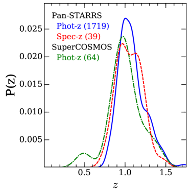
Figure 14.— Smoothed redshift probability distribution functions for clusters with spectroscopic redshifts (red dashed) and photometric redshifts from Spitzer (blue solid) in the Pan-STARRS region, and for those with photometric redshifts from Spitzer (green dot-dashed) in the SuperCOSMOS region. For the spectroscopic redshifts we include clusters with literature redshifts. The functional forms of the spectroscopic and photometric distributions are similar in width and mean redshift for the WISE—Pan-STARRS sample. The SuperCOSMOS photometric redshift distribution is shifted to slightly lower redshift. The secondary peak in the SuperCOSMOS redshift distribution at $z\simeq 0.5$ is due to the combination of lower fidelity rejection of low-redshift galaxies and omission for this catalog of the $z\geq 0.6$ prior used for the WISE—Pan-STARRS photometric redshifts. These smoothed distributions are generated using Gaussian kernel density estimation.

VI.3. Richness

At a fundamental level, there are strong indications that robust cluster mass estimates are attainable directly from observations of the stellar content. Authors including Girardi et al. (2000) and Lin et al. (2003) provided early demonstrations that total baryon content scales with cluster mass. Lin et al. (2003) for example found that the scatter in the relation between $K-$band luminosity ($L_{K}$) and $M_{500}$ from X-ray data was $\sim 45$%, with this scatter dominated by observational uncertainties. More recently, studies with much higher fidelity data and membership information have demonstrated convincingly that the intrinsic scatter is quite low. For example, Mulroy et al. (2014) determined that for the LoCuSS cluster sample the intrinsic scatter in the $L_{K}-M_{500}$ relation is $\sim 10$%. Consistent with these observations, multiple groups have also shown that at a fixed halo mass the ratio of gas mass in the ICM to stellar mass displays a remarkably small intrinsic scatter, indicative of the baryons being partitioned between these two phases with little variation between clusters at fixed $M_{500}$ (Laganá et al., 2008; Zhang et al., 2011; Gonzalez et al., 2013).

The challenge however lies in the reality that in contrast with the LoCuSS sample, membership information is not available for existing cluster surveys directly from the searches. As a result, interlopers can significantly degrade the fidelity of luminosity-based mass estimators. Cluster richnesses, defined based upon number counts rather than total luminosity, are more robust to such contamination. In recent years multiple groups have shown that it is possible to define richness measures that are robust mass proxies with low scatter (e.g., Rykoff et al., 2012; Rozo & Rykoff, 2014; Andreon, 2015; Old et al., 2015; Andreon, 2016, and references therein). Using mock galaxy catalogs to compare a suite of richness estimators, Old et al. (2015) find a scatter of 0.18 dex in the $M_{200}$$-$richness relation for the best proxy. For samples of real, low-redshift clusters, Andreon (2015) and Rozo & Rykoff (2014) define richness measures $n_{200}$ and $\lambda$, for which they find scatters of 0.16 dex and $\sim$0.11 dex, respectively.

Our practical goal for MaDCoWS is to develop a similarly low-scatter mass proxy that can be applied to the full catalog. A limitation, as discussed in the previous section, is that the WISE data alone lack the spatial resolution and depth necessary for such a low-scatter estimator. We have therefore proceeded with the alternate approach of calibrating a Spitzer-based richness estimator that can be applied to the large fraction of the sample with IRAC data from either the archive or our programs in Cycles 9, 11, and 12.

VI.3.1 Richness Definition

For MaDCoWS  we explored use of multiple richness measures to identify a suitable estimator for use with IRAC data. Similar to Rettura et al. (2017), we settled upon use of a fixed aperture for defining the richness. In contrast with that study, we employ a physical rather than angular aperture and incorporate optical data to minimize contamination and reduce scatter in the mass-richness relation.

Our first step in establishing a richness definition for MaDCoWS is to set a uniform limiting [$4.5$] flux density for the IRAC input galaxy catalog of 15 $\mu$Jy ($m=17.7$ Vega). This 4.5$\mu$m-selection is designed to yield an approximately constant stellar mass threshold at $0.7<z<1.5$ and hence minimize the redshift dependence of the richness measure. For this redshift range, 15 $\mu$Jy corresponds to a stellar mass of $\sim 5\times 10^{10}$ M_⊙ assuming an FSPS model with a Chabrier IMF normalized to Coma, with only a modest dependence on star formation history. We also match all 4.5$\mu$m-selected sources to the Pan-STARRS PV2 catalog to obtain $i-$band magnitudes or upper limits for each galaxy.

A challenge that one encounters when using Spitzer imaging for this analysis is that the IRAC field-of-view extends to only $\sim 1.3$ Mpc from the center of the cluster for a galaxy cluster at $z\simeq 1$. One consequence is that the total galaxy density does not necessarily reach the field level within the IRAC field-of-view (for example, see Wylezalek et al., 2013), precluding robust local background subtraction. For this reason, when calculating richnesses we use color cuts to minimize foreground contamination, and then use data from the Spitzer Deep, Wide-Field Survey (SDWFS; Ashby et al., 2009) to estimate the background density. We isolate galaxies near the cluster redshift by combining an $i-$[$3.6$] criteria with a second color cut in [$3.6$]$-$[$4.5$]. This additional cut helps compensate for the fact that the Pan-STARRS imaging is not deep enough to detect all IRAC-selected cluster galaxies at $z=1$.

Starting with the redshift for a given cluster, we use EzGal to calculate the expected $i-$[$3.6$] and [$3.6$]$-$[$4.5$] color for a cluster galaxy. We calculate this color using the same passively evolving model as in §VI.1. We then consider galaxies to be possible cluster members if they are either detected in $i$ and less than one mag bluer in $i-$[$3.6$] than the fiducial color, or else are non-detections in $i$ and the lower limit on $i-$[$3.6$] is no more than one mag redder than the fiducial color. We additionally require that a galaxy have a [$3.6$]$-$[$4.5$] color within $\pm 0.15$ mag of the fiducial. The $i-$[$3.6$] color threshold is set such that this threshold will retain not only passive galaxies, but also star-forming galaxies with exponentially declining star formation histories ($\tau=1$ Gyr) and initial formation redshifts $z_{f}\gtrsim 3$. The width of the color window in [$3.6$]$-$[$4.5$] minimizes exclusion of cluster members due to either photometric uncertainty or redder colors arising from moderate AGN contributions to the photometry, while still providing a meaningful reduction of the background contribution. Examples of the implemented color cuts are shown in Figure 15 for two confirmed MaDCoWS clusters at $z=0.99$ and $z=1.189$, respectively. The boxes in Figure 15 illustrate the color windows used for galaxies with $i-$band detections.

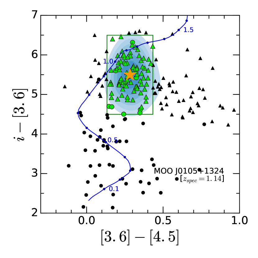
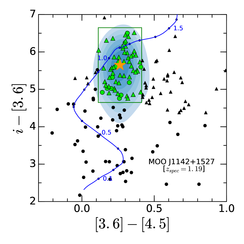
Figure 15.— Color-color diagrams for confirmed clusters MOO J0105+1324 ($z=1.143$; $M_{500}=4.03^{+0.48}_{-0.45}\times 10^{14}$ M_⊙, Gettings et al., 2012) and MOO J1142+1527 ($z=1.189$; $M_{500}=5.45^{+0.58}_{-0.51}\times 10^{14}$ M_⊙; Gonzalez et al., 2015). The symbols and shading are the same as described in Figure 12, with the following exceptions. In this Figure green points correspond to galaxies that are included in calculating the richness based upon their color and physical distance from the cluster centroid ($<1$ Mpc). The solid green lines further indicate the region in color space used to identify galaxies as possible cluster members. The color criteria are designed to retain cluster members while minimizing contamination. When calculating the cluster richness, counts within the SDWFS field are used to apply a statistical background correction. The smoothed density distribution used to determine the cluster redshift and color centroid is shown as the blue color map, as in Figure 12.

A second consequence of the field-of-view constraint is that the data do not uniformly reach to sufficiently large radii for us to use richness estimators extending to $r_{200}$– motivating our use of a fixed, 1 Mpc radius metric aperture. Green points in Figure 12 denote galaxies that lie within 1 Mpc of the WISE-based cluster centroid and satisfy the color criteria. In defining the color cuts and apertures size, we use the photometric redshifts described in §VI.1.

We define the richness $\lambda=N-N_{\mathrm{field}}$, where $N$ is the total number of color-selected galaxies within the metric aperture. In quoting values of $\lambda$ we also include as a subscript the threshold flux density, such that $\lambda_{15}$ denotes the richness calculated for sources $f_{4.5}>15\mu$Jy. For each cluster we calculate the expected field density, $N_{\mathrm{field}}$, by computing the average density of galaxies found in SDWFS for the same magnitude and color cuts and scaling to the appropriate aperture area. In cases where the IRAC data are incomplete within the metric aperture, we apply a correction to account for the fractional area lost. We refrain however from quoting richnesses for clusters at $z<0.7$. For these clusters a 1 Mpc radius extends beyond the field of the IRAC imaging, and a fractional area correction would generally lead to a poor estimate of the true richness. For clusters with archival Spitzer data, we also avoid quoting richnesses for systems with low partical IRAC coverage. Richnesses are included in the catalog in Table LABEL:tab:panstarrsclusters.

The caveat with this approach is that photometric redshift scatter will increase the scatter between richness and mass, and a catastrophic failure on the photometric redshift will result in a spurious richness estimate. As discussed in the Appendix, we find that the former effect is minor. Based upon our spectroscopic confirmation, catastrophic outliers are also rare (at the few percent level). When they do occur, the impact will be a mis-estimation of the richness due to shifting of the color-selection window away from the appropriate cluster color.

VI.3.2 The Relation Between Richness and Mass

To provide an initial calibration of the mass-richness relation we consider a subset of MaDCoWS clusters imaged with Spitzer with derived SZ mass estimates from CARMA. The $M_{500}$ measurements are for a total of 14 clusters, five of which have previously reported SZ detections in Brodwin et al. (2015) and Gonzalez et al. (2015). For previously reported clusters we use updated mass estimates from Decker et al. (2018), which will provide a homogenous analysis for the full sample. The list of clusters used for this analysis is presented in Table 2.

Table 2Clusters in Mass-Richness Calibration

Name	$z$	$\lambda_{15}$	$M_{500}$
			($10^{14}$ M⊙)
MOO J0037+3306	1.139	54$\pm$8	$2.34^{+0.65}_{-0.63}$
MOO J0105+1324	1.143	87$\pm 10$	$4.03^{+0.48}_{-0.45}$
MOO J0123+2545	1.229	41$\pm 7$	$3.90^{+0.89}_{-0.81}$
MOO J0319-0025	1.194	34$\pm$6	$3.11^{+0.53}_{-0.47}$
MOO J1014+0038	1.230	44$\pm$7	$3.26^{+0.32}_{-0.30}$
MOO J1111+1503	1.36	33$\pm$6	2.08${}^{+0.30}_{-0.31}$
MOO J1142+1527	1.189	58$\pm$8	$5.45^{+0.58}_{-0.51}$
MOO J1155+3901	1.009	33$\pm$6	$2.61^{+0.56}_{-0.55}$
MOO J1231+6533	0.99	50$\pm$8	$4.69^{+1.24}_{-1.00}$
MOO J1335+3004	0.984	30$\pm$6	$1.38^{+0.75}_{-0.74}$
MOO J1514+1346	1.059	73$\pm$9	$1.89^{+0.68}_{-0.79}$
MOO J1521+0452	1.312	47$\pm$7	$3.65^{+1.03}_{-0.94}$
MOO J2206+0906	0.951	54$\pm$8	$2.66^{+0.93}_{-0.74}$
MOO J2231+1130	0.80	49$\pm$8	$4.38^{+1.51}_{-1.37}$

Note. — We list in this table all clusters that are included in determination of the mass-richness calibration. All $M_{500}$ measurements are derived from CARMA SZ observations.

We derive a best fit mass-richness relation, which we parameterize as

$$\log\frac{M_{500}}{10^{14}M_{\odot}}=\alpha\log\lambda_{15}+\beta,$$ (2)

using the python implementation of the Bayesian code linmix (Kelly, 2007). For the sake of uniformity, the richnesses used in this fit are calculated using the photometric redshifts to define the appropriate color window for selecting cluster members. We show the data, with richness calculated within a 1 Mpc diameter aperture, in the left panel of Figure 16. The scatter between mass and richness is large for the full ensemble; however, we note that two of these clusters, MOO J0105$+$1323 and MOO J2206$+$0906, are clearly early-stage major mergers based upon Chandra observations that will be presented in a forthcoming paper. These two clusters are plotted as red open circles in the right panel of this figure. A third cluster, MOO J1514$+$1346 (red filled circle), which has the second highest Spitzer-derived richness of the clusters in the Figure, also shows tentative evidence of major merger activity. In the right panel we additionally plot in blue the clusters with existing Chandra data that exhibit no evidence for early-stage major merger activity. Overlaid, we show a best fit mass-richness relation derived excluding the red points.The best-fit relation is plotted as a solid line, with the shaded region indicating the 1$\sigma$ confidence interval.

The best-fit values, which are not well-constrained given the limited dynamic range in mass and small sample size, are formally $\alpha=1.65^{+1.45}_{-0.96}$ and $\beta=-2.16^{+1.57}_{-2.38}$. The scatter in mass about the relation is $36\pm 11$% ($\sigma_{\log M|\lambda}=0.12$), where the quoted uncertainty is derived via a bootstrap resampling of the data. It is clear from the right panel of Figure 16 that a single cluster, MOO J0037+3306, is a significant contributor to this scatter. If we assume that this cluster, for which we currently lack Chandra data, is also a merging cluster, then we can re-fit the data and obtain a refined estimate of the scatter for the other systems that lack similar evidence of ongoing major mergers. Doing so, the best-fit parameters change minimally ($\alpha=1.86^{+1.53}_{-0.88}$ and $\beta=-2.49^{+1.43}_{-2.50}$), while the scatter is reduced to $16\pm 6$% ($\sigma_{\log M|\lambda}=0.07$).

To assess the sensitivity of this relation to photometric redshift uncertainties, positional offsets, and flux density thresholds, we repeat the above analysis varying these quantities. First, we use spectroscopic redshifts, which are available for all but three of these clusters. The change in the richnesses is minimal and hence the fit and $\sigma_{\log M|\lambda}$ remain essentially unchanged. Second, we use the Spitzer-derived centers instead of the WISE cluster centers, again finding negligible change in $\sigma_{\log M|\lambda}$. Finally, we also test the use of a 10$\mu$Jy rather than 15$\mu$Jy threshold for the richness. This again does not appreciably alter the scatter, though it by definition does change the normalization of the relation.

It thus appears, perhaps not surprisingly, that there may exist a relatively tight underlying relation between mass and richness for non-merging clusters, while a subset of merging systems are offset to lower SZ mass (or higher richness) than one would expect from this relation. Multiple studies (e.g. Poole et al., 2007; Krause et al., 2012; Yu et al., 2015) find in simulations that major mergers can systematically bias downward the masses inferred from $Y_{SZ}$. This bias is on average $\sim 10-15$% for $M_{200}$ in Krause et al. (2012), but in some cases can be significantly larger. Physically, this bias is due to the time required for the temperature to increase to the equilibrium level corresponding to the mass of the merged cluster. If the richness measure approaches the new level more quickly than the temperature, which is expected given the large 1 Mpc radius metric aperture used in this paper, then there will also be an offset of merging systems in the $\lambda_{15}-$$M_{500}$ plane.

The MaDCoWS clusters with the highest Spitzer richnesses will therefore be comprised of a combination of the most massive clusters and those undergoing major mergers. ICM observations are necessary to discriminate between these two scenarios. It should also thus be expected that as major mergers become an increasing fraction of the total cluster population with increasing redshift, the observed scatter between SZ mass and richness will increase commensurately unless one identifies and exclude mergers.

We caution that the above is preliminary, being based upon a small number of clusters and not including CARMA non-detections. It therefore should be taken as indicative of the general trend rather than a definitive measure of the mass-richness relation. Ongoing SZ programs with ALMA (PI: Brodwin, programs #2016.2.00014.S and #2017.1.00961.S), MUSTANG-2 (PI: Brodwin, programs GBT 18A-272 and GBT 18B-215), and NIKA2 (PI: Brodwin, programs 095-17 and 095-18), plus a more thorough analysis of the CARMA observations including non-detections and stacking, are forthcoming. These efforts should yield a superior calibration and a better assessment of the total scatter.

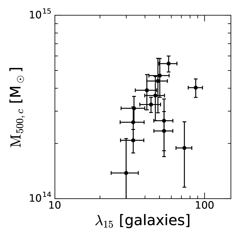
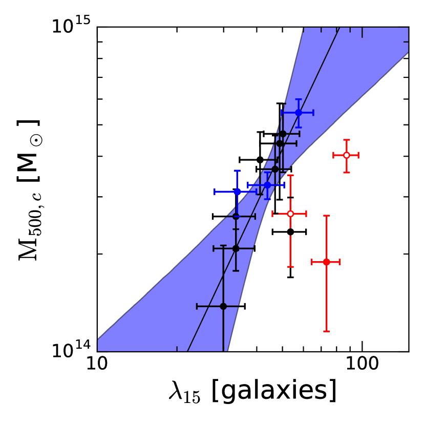
Figure 16.— $Left:$ SZ-based $M_{500}$ versus $\lambda_{15}$, where $\lambda_{15}$ is defined as the number of galaxies within a 1 Mpc aperture centered on the cluster above a flux density threshold of 15$\mu$Jy. For all clusters we use the photometric redshifts to derive the richness; use of the spectroscopic redshifts has a negligible impact on the resulting richnesses. $Right:$ The same as in the left panel, except that systems that are known (likely) major mergers based upon Chandra observations are denoted as open (solid) red points and those with no evidence of major mergers from Chandra observations are plotted as blue points. This panel also includes a best-fit relation is derived excluding the known and likely major mergers. The best-fit relation is shown as a solid black line, while the shaded region denotes the 68% confidence interval. The dispersion in the relation is $\sigma_{\log M|\lambda}=0.12$, or $\sigma_{\log M|\lambda}=0.07$ if one excludes MOO J0037+3306.

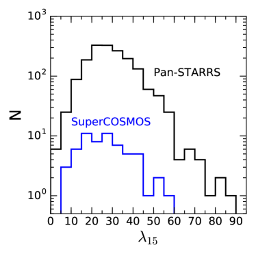
Figure 17.— Histograms showing the distribution in $\lambda_{15}$ for all MaDCoWS clusters with IRAC photometry. The black histogram is for clusters from the WISE—Pan-STARRS region, while the blue histogram is for clusters from the southern WISE—SuperCOSMOS region. Both samples have similar median richnesses and richness distributions.

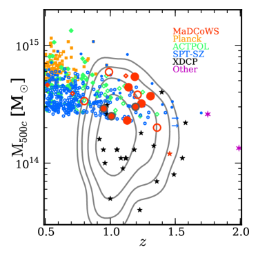
Figure 18.— Comparison in the mass-redshift plane of MaDCoWS clusters with those of other wide-area cluster surveys, including Planck (Planck Collaboration 2014), ACTPol (Hilton et al., 2018) and the South Pole Telescope Sunyaez-Zel’dovich effect survey (SPT-SZ Reichardt et al., 2013; Bleem et al., 2015). For ACTPol we use the M${}_{500c}^{Cal}$ masses, which are scaled by a weak lensing mass calibration factor. The MaDCoWS  clusters shown are those with existing SZ-based masses from CARMA (Brodwin et al., 2015; Gonzalez et al., 2015; Decker et al., 2018), SPT-SZ (Bleem et al., 2015), ACTPol (Hilton et al., 2018), or X-ray-based masses for clusters from the XMM-Newton Distant Cluster Project (XDCP Fassbender et al., 2011a). Filled circles denote clusters with spectroscopic redshifts (including those from Khullar et al. 2018 for SPT); open circles indicate photometric redshifts for all surveys. There are several MaDCoWS clusters from early versions of the search that were confirmed, but did not make the final Pan-STARRS selection due to detection amplitude, masking, or Galactic plane restrictions. We denote these clusters with grey circles around the solid red points. For SPT, the clusters with lower limits on the redshifts are denoted by arrows. We also include XLSSU J021744.1-034536 (Mantz et al., 2014, 2017, $z=1.99$) and IDCS J1426.5+3508 (Stanford et al., 2012, $z=1.75$) as the highest redshift clusters with published SZ masses and redshifts. Finally, we note that MaDCoWS clusters previously detected in the other samples are plotted as red symbols in the marker style corresponding to data points from the other survey. The Planck cluster detected by MaDCoWS has no published mass and is therefore not shown. The contours show the estimated distribution of the full MaDCoWS sample using photometric redshifts and richness-based mass estimates via the mass-richness relation presented in section VI.3.2. The contour spacing corresponds to factor of two changes in the number of clusters per unit redshift and $\log$ mass ($dN/dz/d\log M$). Considering the $1\sigma$ confidence interval on the mass-richness relation, the median mass of the MaDCoWS sample is $M_{500}$$\simeq 0.9-2.2\times 10^{14}$ M_⊙. These contours represent an extrapolation of the mass-richness relation for $M_{500}$$<1.5\times 10^{14}$ M_⊙. They should therefore be considered as only illustrative of the expected full distribution and interpreted with caution. The MaDCoWS sample likely extends down to similar masses as are reached by deep X-ray studies, and probes lower masses than current or planned SZ surveys.

VI.4. Mass and Richness Distributions of MaDCoWS Clusters

In Figure 17 we plot the observed richness distribution for all clusters with IRAC photometry from both the WISE—Pan-STARRS and southern WISE—SuperCOSMOS searches. In both instances these histograms correspond to peak amplitude-limited subsamples, modulo the inclusion of a small number of clusters added from the Spitzer archive. As is evident from the figure, both samples have similar median richnesses and approximately power law distributions at higher richness, as might be expected if the distribution is probing the halo mass function at the high richness end with the survey selection function yielding a turnover in the number of clusters below $\lambda_{15}\sim 25$. Using the mass-richness calibration derived in section VI.3, the median richness for the WISE—Pan-STARRS sample corresponds to a mass $M_{500}$$=1.6^{+0.7}_{-0.8}\times 10^{14}$ M_⊙. The equivalent number for the WISE–SuperCOSMOS sample is $M_{500}$$=1.4\pm 0.7\times 10^{14}$ M_⊙.

We also present in Figure 18 the current distribution in the mass-redshift plane of all MaDCoWS clusters with masses from CARMA or the literature (Fassbender et al., 2011b; Bleem et al., 2015; Hilton et al., 2018), comparing to existing wide-area SZ and X-ray surveys. We denote with open circles clusters for which we currently lack a spectroscopic redshift. These clusters are placed at their estimated photometric redshift. It is apparent from Figure 18 that the MaDCoWS sample includes clusters that span the mass range probed by the combination of existing SZ and X-ray surveys at this epoch, including several of the most massive clusters known at $z>1$. For comparison, we also plot contours showing the inferred distribution for all MaDCoWS clusters with IRAC photometry, where we use the photometric redshifts from §VI.2 and richness-based mass estimates from §VI.3. The density contours are spaced by powers of two, illustrating that the distribution is strongly peaked at $z\simeq 1$ and $M\simeq 1-2\times 10^{14}$ M_⊙. We caution against over-interpretation of these contours, particularly outside the range over which the mass-richness relation is calibrated ($M_{500}$$\sim 1.5-5.4\times 10^{14}$ M_⊙). These contours should be considered illustrative rather than definitive.

VI.5. Comparison with ACTPol

As a test of our ability to recover known massive, high-redshift clusters, we compare our MaDCoWS—Pan-STARRS results with the two-season ACTPol Sunyaev-Zel’dovich catalog (Hilton et al., 2018). ACTPol, which covers 987.5 deg², is the only published high-redshift SZ survey that overlaps with the WISE—Pan-STARRS region. The ACTPol catalog includes 19 clusters at $z>0.9$, four of which have spectroscopic redshifts, with weak-lensing calibrated masses $M^{Cal}_{500}\gtrsim 2.5\times 10^{14}$ M_⊙. Of these 19 ACTPol clusters, only one (ACT-CL J0125.2-0802) is in the MaDCoWS catalog in Table LABEL:tab:panstarrsclusters. We investigate the cause of this minimal overlap, finding that it can be attributed to several factors. A minor factor is masking of bright stars in the MaDCoWS search, which removes one of the 19 clusters (ACT-CL J0248.7-0019). The other two more significant factors are the high threshold for our catalog and the large scatter between peak amplitude and mass – the latter also being the reason that IRAC imaging is required for determining richnesses. Two additional clusters are detected at SNR$>8$, but just below our peak amplitude threshold, and a total of 8 (12) out of the 18 unmasked clusters are detected at SNR$>5$ ($>3$). From a practical perspective, using the current approach it would not be possible to identify these clusters as the most massive among the larger ensemble of MaDCoWS clusters in this region without deeper mid-infrared imaging such as we have obtained with Spitzer/IRAC for a subset of the MaDCoWS clusters.

VI.6. Future Improvements

The current MaDCoWS search attempts to make optimal use of existing surveys, but there are several prospects for upcoming data sets that can yield an improved version of the MaDCoWS search. One notable limitation of the current search is the limited depth of the SuperCOSMOS imaging outside the Pan-STARRS footprint. As described in §II.2.3, the shallowness of this imaging yields higher foreground contamination (Fig. 3), resulting in a lower fidelity and lower median redshift catalog at $\delta<-30$. Several surveys are underway that will enable a uniform search comparable in quality to what is currently achieved in the Pan-STARRS region over the full extragalactic sky. Observations for the DES (Dark Energy Survey Collaboration et al., 2016) are expected to provide adequate data over $\sim 5000$ deg², of which over half are at $\delta<-30^{\circ}$. Of particular note, this area includes the region of the SPT-SZ survey (Bleem et al., 2015), enabling us to compare catalogs and better assess selection biases associated with the MaDCoWS search. Two other surveys that also have the potential to enable a higher fidelity search in the south are the SkyMapper Southern Sky Survey Main Survey (SMSS, Keller et al., 2007) and the Southern Photometric Local Universe Survey (S-PLUS). The SMSS is designed to cover the entire southern sky ($\delta<0^{\circ}$) to $u,g,v,r,i,z=20.5,20.5,21.7,21.7,20.7,19.7$ (AB, $5\sigma$). These data will significantly improve rejection of low-redshift galaxies relative to the $R_{F}$ limit used for SuperCOSMOS, although the $i-$band depth is still shallow relative to Pan-STARRS. S-PLUS meanwhile plans to cover $\sim 8000$ deg² in $ugriz$ and seven narrow-band filters. S-PLUS is designed to have shallower $i$-band photometry than Pan-STARRS  but is expected to be sufficiently deep in $z-$band to enable an equivalent search.

A more fundamental limitation for the current MaDCoWS search is the depth of the WISE photometric catalog that is used for the initial selection of galaxies. As was shown in Figure 1, the WISE photometry is only currently deep enough to identify at $>5\sigma$ individual $\sim$$L^{\ast}$ galaxies out to $z\simeq 1$ in W1, and only detects these galaxies at $\sim 2\sigma$ in W2. This depth threshold has multiple implications for the search. First, it necessitates that we use W1 for galaxy selection, reducing the sensitivity of the survey to the highest redshift clusters. Second, because we are only detecting the bright end of the luminosity function with WISE, cluster identification relies upon extracting a cluster signal generated by a small number of bright galaxies. The strength of the signal is therefore highly sensitive to statistical variations in the number counts of cluster galaxies, which can rise due to both blending of individual sources at the resolution of WISE and statistical variations in the luminosity function. Thus, while detections in the current survey catalog result from true overdensities, not all overdensities are detected as significant due to such statistical variance.

There exists the potential for significant improvement on this front. For this paper we have used the AllWISE catalog. This catalog, which was released in 2013, is the deepest currently available all-sky WISE catalog and incorporates all data prior to the end of the post-cryogenic mission in February 2011. During this period WISE mapped the full sky twice in the short wavelength bands. In October 2013 the WISE satellite was reactivated for the NEOWISE mission (Mainzer et al., 2014), resuming survey observations in W1 and W2. The mission is currently scheduled to continue through December 2018, providing a factor of five or more increase in total exposure time in these bands over the full sky, and thus a factor of five increase in the total exposure time relative to AllWISE images. Meisner et al. (2017) have demonstrated the potential gain in depth. Stacking three years worth of data from WISE and NEOWISE, they reach 0.56 (0.46) mag deeper in W1 (W2) than AllWISE data alone. The “CatWISE” effort, funded by NASA’s Astrophysics Data Analysis Program, is adapting the AllWISE data processing pipeline to generate a catalog from four years of WISE and NEOWISE data, with planned release in mid-2019. Galaxy catalogs derived from full-depth stacks from the entire WISE and NEOWISE missions will have sufficent depth to detect $L^{\ast}$ galaxies in W2 out to $z\gtrsim 2$ and push much fainter than $L^{\ast}$ in W1, enabling a higher completeness cluster search at $z\sim 1$ and greater sensitivity to high-redshift ($z\simeq 1.5-2$) clusters.

Finally, from an algorithmic perspective, the increased sensitivity of CatWISE, coupled with the optical surveys, will enable a more sophisticated treatment of foreground rejection and should enable a detection observable that is a significantly lower scatter proxy for cluster mass. The combination of a full-depth CatWISE catalog and the upcoming southern optical surveys together thus hold promise for a uniform, high-fidelity cluster search extending to $z>1.5$ and spanning the full extragalactic sky.

VII. Summary

The Massive and Distant Clusters of WISE Survey (MaDCoWS) is a program designed to identify massive galaxy clusters at $z\simeq 1$ over the full extragalactic sky using the combination of WISE imaging and ground-based optical photometry. MaDCoWS uses the combination of optical rejection and infrared color-selection to isolate a 3.4$\mu$m flux-limited population of galaxies at $z\gtrsim 0.8$, and then to search for overdensities on the expected physical scale of galaxy clusters at $z\sim 1$. This approach provides a large, wide-area sample of massive galaxy clusters at $z\simeq 1$ for evolutionary studies, and allows the most massive galaxy clusters at this epoch to be identified over the full extragalactic sky.

The primary MaDCoWS search covers the full extragalactic footprint of Pan-STARRS ($\delta>-30^{\circ}$). This search uses the AllWISE catalog coupled with Pan-STARRS $i-$band photometry to effectively identify galaxy clusters at $0.7\lesssim z\lesssim 1.5$. The resultant catalog, which includes $2433$ cluster candidates, is presented in Table LABEL:tab:panstarrsclusters. These clusters are selected based upon the peak amplitude in the cluster detection maps and all have SNR$>8$.

We conduct a complementary MaDCoWS search outside the Pan-STARRS footprint using the combination of WISE data and shallower SuperCOSMOS $r-$band photometry. This search yields $250$ cluster candidates, which are presented in Table 4. The main limitation of this catalog, as discussed in the §III.2.1, is that it is more prone to contamination from lower-redshift clusters and chance projections due to the less efficient removal of low-redshift galaxies.

For the primary WISE—Pan-STARRS search, we have obtained follow-up Spitzer observations for $1723$ clusters, enabling us to derive photometric redshifts and richness estimates. Using a subset of 38 clusters with spectroscopic redshifts and IRAC imaging, we find that these redshifts have an uncertainty of $\sigma_{z}/(1+z)=$0.036. The median photometric redshift for the ensemble is $z=1.06$, and all photometric redshifts lie at $z>0.7$. Similarly, photometric redshifts based upon Spitzer and DES observations for $64$ clusters imply a median redshift of $z=0.98$, with 94% of candidates at $z>0.7$.

Sunyaev-Zel’dovich mass estimates for a subset of 14 clusters also enables us to derive an initial mass-richness relation for the MaDCoWS sample. We find that the distribution of masses and redshifts is consistent with the majority of clusters obeying a tight relation ($\sigma_{\log M|\lambda}=0.06$), with a subset of merging systems offset to higher richness (or equivalently lower mass). Based upon this relation, we estimate that the median mass of the WISE—Pan-STARRS  and WISE—SuperCOSMOS catalogs are $M_{500}$$=1.6^{+0.6}_{-0.7}\times 10^{14}$ M_⊙ and $M_{500}$$=1.4\pm 0.7\times 10^{14}$ M_⊙, respectively.

Finally, we compare in the mass-redshift plane the distribution of MaDCoWS clusters with other existing cluster samples (Figure 18). The MaDCoWS sample extends to comparably high redshifts as the published Sunyaev-Zel’dovich samples from ACT and SPT, while probing a range in cluster mass similar to the XDCP survey but over a much larger area.

Looking forward, the additional observations from the NEOWISE mission incorporated into the CatWISE catalog, coupled with upcoming data releases from southern optical surveys together promise to enable a second generation MaDCoWS search extending towards $z\sim 2$ and covering the full extragalactic sky. This second generation search will complement eROSITA and next generation SZ surveys.

Table 3Top $2433$ Candidate Clusters in the WISE—Pan-STARRS Region

Cluster	$\alpha$	$\delta$	Peak	SNR	$z_{phot}$	$z$ (Members)	$\lambda_{15}$	$M_{500}$	Spitzer	Literature Names	Ref.
	[J2000]	[J2000]	Height					[$10^{14}\mathrm{M}_{\odot}$]		& Comments
MOO J0001+1428	00h01m09.1s	14d28m57s	0.59	9.0	$1.14^{+0.13}_{-0.10}$	$\cdots$	$15\pm 4$	$\cdots$	C11	$\cdots$
MOO J0001+3644	00h01m09.8s	36d44m38s	0.56	9.9	$\cdots$	$\cdots$	$\cdots$	$\cdots$	$\cdots$	$\cdots$
MOO J0001+3440	00h01m38.5s	34d40m50s	0.56	9.3	$\cdots$	$\cdots$	$\cdots$	$\cdots$	$\cdots$	$\cdots$
MOO J0001$-$2447	00h01m49.4s	-24d47m32s	0.58	8.4	$\cdots$	$\cdots$	$\cdots$	$\cdots$	$\cdots$	$\cdots$
MOO J0001$-$2533	00h01m54.7s	-25d33m35s	0.69	10.6	$1.17^{+0.06}_{-0.05}$	$\cdots$	$43\pm 6$	$\cdots$	C11	$\cdots$
MOO J0002$-$0820	00h02m06.2s	-08d20m50s	0.56	8.5	$\cdots$	$\cdots$	$\cdots$	$\cdots$	$\cdots$	$\cdots$
MOO J0002+1751	00h02m29.5s	17d51m30s	0.60	9.5	$1.33^{+0.04}_{-0.06}$	$\cdots$	$26\pm 5$	$\cdots$	C11	$\cdots$
MOO J0003$-$0903	00h03m01.2s	-09d03m24s	0.66	10.0	$0.94^{+0.07}_{-0.06}$	$\cdots$	$18\pm 5$	$\cdots$	C11	$\cdots$
MOO J0003$-$2925	00h03m28.3s	-29d25m58s	0.84	12.9	$1.05^{+0.10}_{-0.10}$	$\cdots$	$22\pm 5$	$\cdots$	C11	$\cdots$
MOO J0003$-$1341	00h03m37.3s	-13d41m16s	0.69	10.5	$0.85^{+0.06}_{-0.05}$	$\cdots$	$32\pm 6$	$\cdots$	C11	$\cdots$
MOO J0004$-$0232	00h04m26.7s	-02d32m44s	0.56	8.5	$\cdots$	$\cdots$	$\cdots$	$\cdots$	$\cdots$	$\cdots$
MOO J0004+0024	00h04m42.8s	00d24m00s	0.57	8.7	$\cdots$	$\cdots$	$\cdots$	$\cdots$	$\cdots$	$\cdots$
MOO J0004+0108	00h04m52.1s	01d08m36s	0.61	9.3	$0.94^{+0.09}_{-0.09}$	$\cdots$	$21\pm 5$	$\cdots$	C11	$\cdots$
MOO J0005+1329	00h05m28.6s	13d29m32s	0.58	8.8	$0.94^{+0.08}_{-0.08}$	$\cdots$	$34\pm 6$	$\cdots$	C11	$\cdots$
MOO J0005+0024	00h05m29.2s	00d24m00s	0.56	8.6	$\cdots$	$\cdots$	$\cdots$	$\cdots$	$\cdots$	$\cdots$
MOO J0005+1408	00h05m37.8s	14d08m10s	0.69	10.4	$0.98^{+0.06}_{-0.06}$	$\cdots$	$17\pm 5$	$\cdots$	C11	$\cdots$
MOO J0005$-$0443	00h05m40.1s	-04d43m26s	0.57	8.6	$\cdots$	$\cdots$	$\cdots$	$\cdots$	$\cdots$	$\cdots$
MOO J0006+3050	00h06m29.3s	30d50m55s	0.65	10.9	$1.02^{+0.06}_{-0.06}$	$\cdots$	$42\pm 7$	$\cdots$	C11	$\cdots$
MOO J0006$-$0244	00h06m34.3s	-02d44m42s	0.57	8.7	$\cdots$	$\cdots$	$\cdots$	$\cdots$	$\cdots$	$\cdots$
MOO J0006$-$0751	00h06m36.3s	-07d51m39s	0.57	8.6	$\cdots$	$\cdots$	$\cdots$	$\cdots$	$\cdots$	$\cdots$
MOO J0007$-$2108	00h07m13.6s	-21d08m36s	0.56	8.4	$\cdots$	$\cdots$	$\cdots$	$\cdots$	$\cdots$	$\cdots$
MOO J0008$-$1703	00h08m16.4s	-17d03m40s	0.56	8.4	$\cdots$	$\cdots$	$\cdots$	$\cdots$	$\cdots$	$\cdots$
MOO J0009$-$0750	00h09m34.3s	-07d50m12s	0.62	9.4	$1.14^{+0.17}_{-0.15}$	$\cdots$	$22\pm 5$	$\cdots$	C11	$\cdots$
MOO J0010+2027	00h10m18.9s	20d27m28s	0.63	10.0	$0.88^{+0.12}_{-0.10}$	$\cdots$	$14\pm 5$	$\cdots$	C11	$\cdots$
					$1.48^{+0.26}_{-0.10}$	$\cdots$	$18\pm 5$	$\cdots$
MOO J0010+3142	00h10m47.7s	31d42m14s	0.66	10.9	$1.41^{+0.05}_{-0.05}$	$\cdots$	$33\pm 5$	$\cdots$	C11	$\cdots$
MOO J0010+2751	00h10m54.1s	27d51m10s	0.58	9.7	$0.98^{+0.10}_{-0.09}$	$\cdots$	$20\pm 5$	$\cdots$	C11	$\cdots$
MOO J0011$-$1414	00h11m14.4s	-14d14m46s	0.60	9.0	$1.03^{+0.08}_{-0.06}$	$\cdots$	$35\pm 6$	$\cdots$	C11	$\cdots$
MOO J0011$-$2530	00h11m31.3s	-25d30m55s	0.56	8.7	$\cdots$	$\cdots$	$\cdots$	$\cdots$	$\cdots$	$\cdots$
MOO J0012$-$0218	00h12m54.4s	-02d18m10s	0.60	9.1	$1.19^{+0.08}_{-0.07}$	$\cdots$	$35\pm 6$	$\cdots$	C11	$\cdots$
MOO J0012$-$1941	00h12m59.5s	-19d41m38s	0.57	8.5	$\cdots$	$\cdots$	$\cdots$	$\cdots$	$\cdots$	$\cdots$
MOO J0013+0700	00h13m48.1s	07d00m52s	0.59	8.9	$1.09^{+0.07}_{-0.07}$	$\cdots$	$33\pm 6$	$\cdots$	C11	$\cdots$
MOO J0014$-$0909	00h14m33.3s	-09d09m23s	0.61	9.2	$0.89^{+0.05}_{-0.04}$	$\cdots$	$16\pm 6$	$\cdots$	C11	$\cdots$
MOO J0014$-$0459	00h14m40.5s	-04d59m23s	0.62	9.5	$1.02^{+0.04}_{-0.04}$	$\cdots$	$32\pm 6$	$\cdots$	C9	$\cdots$
MOO J0015+2059	00h15m06.2s	20d59m58s	0.57	9.1	$\cdots$	$\cdots$	$\cdots$	$\cdots$	$\cdots$	$\cdots$
MOO J0015+2822	00h15m06.3s	28d22m16s	0.59	9.9	$0.98^{+0.10}_{-0.09}$	$\cdots$	$27\pm 5$	$\cdots$	C11	$\cdots$

Table 4Candidate Clusters in the WISE—SuperCOSMOS region with Spitzer imaging

Cluster	$\alpha$	$\delta$	Peak	SNR	$z_{phot}$	$\lambda_{15}$	$M_{500}$	Literature Names	Ref.
	[J2000]	[J2000]	Height				[$10^{14}\mathrm{M}_{\odot}$]	& Comments
MOO J0002$-$3118	00h02m12.2s	-31d18m18s	0.66	8.7	$\cdots$	$\cdots$	$\cdots$	$\cdots$
MOO J0002$-$3419	00h02m24.6s	-34d19m32s	0.71	9.3	$1.42^{+0.05}_{-0.05}$	$17\pm 4$	$\cdots$	$\cdots$
MOO J0003$-$7017	00h03m11.9s	-70d17m39s	0.66	9.5	$\cdots$	$\cdots$	$\cdots$	$\cdots$
MOO J0003$-$4725	00h03m21.9s	-47d25m48s	0.80	11.0	$1.45^{+0.05}_{-0.05}$	$37\pm 6$	$\cdots$	$\cdots$
MOO J0007$-$3223	00h07m59.5s	-32d23m33s	0.65	8.6	$\cdots$	$\cdots$	$\cdots$	$\cdots$
MOO J0008$-$5332	00h08m07.9s	-53d32m49s	0.65	8.9	$\cdots$	$\cdots$	$\cdots$	$\cdots$
MOO J0008$-$4710	00h08m39.6s	-47d10m27s	0.66	9.0	$\cdots$	$\cdots$	$\cdots$	$\cdots$
MOO J0009$-$7206	00h09m56.2s	-72d06m23s	0.61	8.8	$\cdots$	$\cdots$	$\cdots$	$\cdots$
MOO J0010$-$4652	00h10m49.3s	-46d52m39s	0.64	8.7	$\cdots$	$\cdots$	$\cdots$	$\cdots$
MOO J0011$-$3126	00h11m20.7s	-31d26m37s	0.63	8.4	$\cdots$	$\cdots$	$\cdots$	$\cdots$
MOO J0012$-$4926	00h12m54.8s	-49d26m46s	0.65	8.9	$\cdots$	$\cdots$	$\cdots$	$\cdots$
MOO J0013$-$4452	00h13m57.7s	-44d52m31s	0.65	8.8	$\cdots$	$\cdots$	$\cdots$	$\cdots$
MOO J0016$-$6531	00h16m04.2s	-65d31m49s	0.68	9.8	$\cdots$	$\cdots$	$\cdots$	$\cdots$
MOO J0016$-$3302	00h16m48.4s	-33d02m25s	0.73	9.7	$1.05^{+0.09}_{-0.09}$	$22\pm 5$	$\cdots$	$\cdots$
MOO J0019$-$6803	00h19m23.5s	-68d03m24s	0.69	9.9	$\cdots$	$\cdots$	$\cdots$	$\cdots$
MOO J0021$-$3240	00h21m32.8s	-32d40m22s	0.61	8.1	$\cdots$	$\cdots$	$\cdots$	$\cdots$
MOO J0028$-$4449	00h28m56.1s	-44d49m56s	0.69	9.3	$0.93^{+0.03}_{-0.03}$	$29\pm 6$	$\cdots$	$\cdots$
MOO J0033$-$4629	00h33m15.5s	-46d29m41s	0.61	8.4	$\cdots$	$\cdots$	$\cdots$	$\cdots$
MOO J0033$-$5913	00h33m57.0s	-59d13m50s	0.63	8.6	$\cdots$	$\cdots$	$\cdots$	$\cdots$
MOO J0036$-$7637	00h36m45.8s	-76d37m37s	0.65	9.5	$\cdots$	$\cdots$	$\cdots$	$\cdots$
MOO J0037$-$5318	00h37m38.3s	-53d18m20s	0.65	8.9	$\cdots$	$\cdots$	$\cdots$	$\cdots$
MOO J0038$-$3134	00h38m46.4s	-31d34m48s	0.63	8.3	$\cdots$	$\cdots$	$\cdots$	$\cdots$
MOO J0039$-$3743	00h39m42.2s	-37d43m55s	0.64	8.8	$\cdots$	$\cdots$	$\cdots$	$\cdots$
MOO J0041$-$6154	00h41m56.9s	-61d54m04s	0.62	8.6	$\cdots$	$\cdots$	$\cdots$	$\cdots$
MOO J0042$-$5328	00h42m20.0s	-53d28m50s	0.65	8.9	$\cdots$	$\cdots$	$\cdots$	$\cdots$
MOO J0045$-$5226	00h45m21.4s	-52d26m17s	0.62	8.5	$\cdots$	$\cdots$	$\cdots$	$\cdots$
MOO J0046$-$4510	00h46m21.6s	-45d10m12s	0.64	8.7	$\cdots$	$\cdots$	$\cdots$	$\cdots$
MOO J0048$-$4110	00h48m44.1s	-41d10m16s	0.61	8.3	$\cdots$	$\cdots$	$\cdots$	$\cdots$
MOO J0054$-$3141	00h54m23.9s	-31d41m45s	0.70	9.2	$0.82^{+0.07}_{-0.05}$	$18\pm 6$	$\cdots$	$\cdots$
MOO J0057$-$5107	00h57m34.8s	-51d07m41s	0.62	8.5	$\cdots$	$\cdots$	$\cdots$	$\cdots$
MOO J0100$-$5005	01h00m10.4s	-50d05m46s	0.61	8.4	$\cdots$	$\cdots$	$\cdots$	$\cdots$
MOO J0102$-$3116	01h02m41.5s	-31d16m39s	0.68	8.9	$1.02^{+0.10}_{-0.10}$	$43\pm 7$	$\cdots$	$\cdots$
MOO J0105$-$7752	01h05m01.5s	-77d52m48s	0.66	9.6	$\cdots$	$\cdots$	$\cdots$	$\cdots$
MOO J0105$-$3355	01h05m05.3s	-33d55m25s	0.74	9.8	$0.98^{+0.10}_{-0.10}$	$18\pm 5$	$\cdots$	$\cdots$
MOO J0107$-$3738	01h07m18.6s	-37d38m58s	0.61	8.4	$\cdots$	$\cdots$	$\cdots$	$\cdots$

Note. — This table includes basic information for clusters from the SuperCOSMOS search for which there is existing Spitzer imaging. The columns are similar to Table LABEL:tab:panstarrsclusters with a few notable exceptions. Foremost, the peak height is normalized relative to the most significant peak in the SuperCOSMOS region. It is not directly comparable to the Pan-STARRS peak height column. All quoted richnesses and photometric redshifts in this Table use DES for the optical photometry. This table is available in its entirety in machine-readable form. Finally, the Spitzer column is omitted because all listed clusters have imaging from our Cycle 11-12 program, and the spectroscopic redshift column is omitted due to a lack of spectroscopic confirmation for this sample. References: [1] Bleem et al. (2015).

Table 5Additional Clusters from the Preliminary WISE—SDSS Search

Cluster	$\alpha$	$\delta$	$z_{phot}$	$z$ (Members)	$\lambda_{15}$	$M_{500}$	Literature Names	Ref.
	[J2000]	[J2000]				[$10^{14}\mathrm{M}_{\odot}$]	& Comments
MOO J0005$-$0944	00h05m49.7s	-09d44m00s	$1.49^{+0.26}_{-0.09}$	$\cdots$	$27\pm 5$	$\cdots$
MOO J0012+1602	00h12m13.5s	16d02m48s	$0.97^{+0.03}_{-0.04}$	0.944 (23)	$67\pm 8$	$\cdots$		[1,3]
MOO J0022+0452	00h22m37.5s	04d52m40s	$0.96^{+0.05}_{-0.07}$	$\cdots$	$25\pm 6$	$\cdots$
MOO J0023+0557	00h23m07.6s	05d57m00s	$1.02^{+0.10}_{-0.09}$	$\cdots$	$43\pm 7$	$\cdots$
MOO J0026+1856	00h26m42.4s	18d56m03s	$\cdots$	$\cdots$	$\cdots$	$\cdots$
MOO J0036$-$2111	00h36m31.7s	-21d11m34s	$\cdots$	$\cdots$	$\cdots$	$\cdots$	†
MOO J0045+0919	00h45m34.2s	09d19m14s	$0.81^{+0.07}_{-0.06}$	$\cdots$	$34\pm 6$	$\cdots$
MOO J0045$-$0534	00h45m47.5s	-05d34m12s	$0.97^{+0.09}_{-0.09}$	$\cdots$	$20\pm 5$	$\cdots$
MOO J0121+0353	01h21m41.4s	03d53m08s	$1.29^{+0.05}_{-0.05}$	$\cdots$	$36\pm 6$	$\cdots$
MOO J0123+0752	01h23m02.2s	07d52m19s	$0.93^{+0.07}_{-0.08}$	$\cdots$	$27\pm 6$	$\cdots$
MOO J0134+0122	01h34m03.3s	01d22m45s	$1.28^{+0.06}_{-0.09}$	$\cdots$	$37\pm 6$	$\cdots$
MOO J0140+2913	01h40m07.9s	29d13m35s	$\cdots$	$\cdots$	$\cdots$	$\cdots$	†
MOO J0153$-$0616	01h53m35.7s	-06d16m00s	$0.93^{+0.08}_{-0.08}$	$\cdots$	$36\pm 6$	$\cdots$
MOO J0204$-$1918	02h04m21.2s	-19d18m14s	$1.10^{+0.05}_{-0.04}$	$\cdots$	$47\pm 7$	$\cdots$
MOO J0207+0636	02h07m11.5s	06d36m20s	$0.86^{+0.09}_{-0.06}$	$\cdots$	$30\pm 6$	$\cdots$
MOO J0211+2024	02h11m23.1s	20d24m17s	$1.08^{+0.04}_{-0.05}$	$\cdots$	$45\pm 7$	$\cdots$
MOO J0222+1402	02h22m41.1s	14d02m20s	$0.99^{+0.07}_{-0.06}$	$\cdots$	$20\pm 5$	$\cdots$
MOO J0222$-$0329	02h22m54.4s	-03d29m28s	$1.14^{+0.10}_{-0.08}$	$\cdots$	$30\pm 5$	$\cdots$
MOO J0224$-$0620	02h24m51.8s	-06d20m40s	$1.32^{+0.05}_{-0.07}$	0.816 (7)	$38\pm 6$	$\cdots$	CFHTLENS 362136-6.33379	[2,3]
MOO J0237+2809	02h37m10.8s	28d09m54s	$0.94^{+0.07}_{-0.07}$	$\cdots$	$45\pm 7$	$\cdots$
MOO J0237$-$0806	02h37m46.4s	-08d06m45s	$1.14^{+0.08}_{-0.06}$	$\cdots$	$35\pm 6$	$\cdots$
MOO J0245+2018	02h45m08.4s	20d18m22s	$0.91^{+0.14}_{-0.11}$	0.757 (14)	$19\pm 6$	$\cdots$		[3]
MOO J0313+0014	03h13m35.3s	00d14m40s	$0.97^{+0.12}_{-0.12}$	$\cdots$	$22\pm 5$	$\cdots$
MOO J0319$-$0025	03h19m24.7s	-00d25m24s	$1.21^{+0.07}_{-0.08}$	1.194 (20)	$33\pm 6$	$3.0^{+0.4}_{-0.5}$		[1,3]
MOO J0328$-$0532	03h28m52.5s	-05d32m01s	$0.90^{+0.11}_{-0.09}$	$\cdots$	$17\pm 5$	$\cdots$
MOO J0352+1123	03h52m05.6s	11d23m01s	$1.12^{+0.06}_{-0.07}$	$\cdots$	$37\pm 6$	$\cdots$
MOO J0527+0057	05h27m56.3s	00d57m27s	$0.86^{+0.06}_{-0.04}$	$\cdots$	$53\pm 7$	$\cdots$
MOO J0738+2757	07h38m39.9s	27d57m03s	$1.06^{+0.08}_{-0.07}$	$\cdots$	$29\pm 5$	$\cdots$
MOO J0824+2251	08h24m56.1s	22d51m27s	$0.80^{+0.06}_{-0.05}$	$\cdots$	$21\pm 6$	$\cdots$
			$1.21^{+0.07}_{-0.07}$		$25\pm 6$
MOO J0826+4522	08h26m39.9s	45d22m01s	$1.26^{+0.05}_{-0.08}$	$\cdots$	$37\pm 6$	$\cdots$
MOO J0828+1839	08h28m33.5s	18d39m40s	$0.88^{+0.09}_{-0.08}$	$\cdots$	$4\pm 4$	$\cdots$
MOO J0830+2635	08h30m11.0s	26d35m04s	$1.10^{+0.10}_{-0.09}$	$\cdots$	$22\pm 5$	$\cdots$
MOO J0838+2146	08h38m13.0s	21d46m09s	$0.81^{+0.08}_{-0.07}$	$\cdots$	$12\pm 5$	$\cdots$
			$1.33^{+0.07}_{-0.07}$		$25\pm 5$
MOO J0842+0033	08h42m24.6s	00d33m13s	$0.98^{+0.07}_{-0.06}$	$\cdots$	$47\pm 7$	$\cdots$
MOO J0846+2747	08h46m46.1s	27d47m10s	$1.32^{+0.04}_{-0.06}$	$\cdots$	$36\pm 6$	$\cdots$

Note. — This table lists clusters from the preliminary WISE—SDSS search that are not contained in Table LABEL:tab:panstarrsclusters but for which we have obtained spectroscopic redshifts, SZ masses, or Cycle 9 Spitzer imaging. Some of these clusters were lost due to more conservative masking in the Pan-STARRS search, while others lie below the peak height threshold for Table LABEL:tab:panstarrsclusters. For consistency within the table, we omit the peak height and SNR columns from the previous table. We also omit the column indicating the source of the Spitzer observations, since all clusters were observed in Cycle 9. This table is available in its entirety in machine-readable form. A † in the reference column indicates that there is a foreground cluster along the line of sight. References: [1] Brodwin et al. (2015), [2] Ford et al. (2014, 2015), [3] Stanford et al. (2014), [4] Decker et al. (2018), [5] Wen & Han (2018)

Appendix A Spitzer-only Coordinates, Photometric Redshifts, and Richnesses

For the primary WISE—Pan-STARRS catalog in Table LABEL:tab:panstarrsclusters the quoted photometric redshifts and richnesses are derived using the cluster coordinates derived directly from the cluster search. As discussed in §V.3, for clusters with Spitzer IRAC imaging we also derived centroids using the Spitzer data. For completeness, we list in Table 6 these coordinates. We also present the photometric redshifts and richnesses that one would obtain using these centroids rather than the WISE coordinates. This is intended to enable consistency checks, but we emphasize that Table LABEL:tab:panstarrsclusters should be considered the fiducial catalog for the Pan-STARRS region. In this Table, we only include clusters for which the Spitzer centroiding algorithm was able to successfully recover a peak within 60^′′ of the WISE position, and only include photometric redshifts and richnesses when this association was within 45^′′.

Table 6Quantities Derived Using Spitzer Coordinates for Pan-STARRS Clusters

Cluster	$\alpha_{S}$	$\delta_{S}$	WISE-Spitzer	$z_{phot,S}$	$\lambda_{15,S}$
	[J2000]	[J2000]	Separation[′′]
MOO J0001+1428	00h01m09.75s	14d29m25.4s	29	$1.14^{+0.13}_{-0.10}$	$15\pm 4$
MOO J0001$-$2533	00h01m54.22s	-25d33m21.9s	15	$1.17^{+0.06}_{-0.05}$	$43\pm 6$
MOO J0002+1751	00h02m27.93s	17d51m51.6s	31	$1.33^{+0.04}_{-0.06}$	$26\pm 5$
MOO J0003$-$0903	00h03m01.49s	-09d03m21.5s	5	$0.94^{+0.07}_{-0.06}$	$18\pm 5$
MOO J0003$-$2925	00h03m28.27s	-29d26m07.2s	9	$1.05^{+0.10}_{-0.10}$	$22\pm 5$
MOO J0003$-$1341	00h03m38.64s	-13d41m54.4s	43	$0.85^{+0.06}_{-0.05}$	$32\pm 6$
MOO J0003$-$1341	00h03m38.64s	-13d41m54.4s	43	$0.85^{+0.06}_{-0.05}$	$32\pm 6$
MOO J0005+1329	00h05m28.65s	13d29m28.0s	4	$0.94^{+0.08}_{-0.08}$	$34\pm 6$
MOO J0005+1408	00h05m37.17s	14d08m01.4s	12	$0.98^{+0.06}_{-0.06}$	$17\pm 5$
MOO J0006+3050	00h06m26.82s	30d51m08.9s	34	$1.02^{+0.06}_{-0.06}$	$42\pm 7$

Note. — As discussed in §V.3, for clusters with Spitzer imaging we derived Spitzer-based centroids. We list in this table these centroids and also the alternate photometric redshifts and richness values that result if these centroids are used rather than those from the WISE search. By construction, the Spitzer centroid must lie within 45^′′ of the WISE location. We only quote photometric redshifts ($z_{phot,S}$) and richnesses ($\lambda_{15,S}$) in cases where a Spitzer peak is identified within this distance. This table is available in its entirety in machine-readable form.

Appendix B Spectroscopic Confirmation of PSZ2 G126.57+5161

This paper includes a new spectroscopic redshift for one cluster, PSZ2 G126.57+5161, which appears in our catalog as MOO J1229+6521. PSZ2 G126.57+5161 has a published redshift of $z=0.815$ based upon a single galaxy (Burenin et al., 2018). Here we provide an improved redshift based upon multi-object spectroscopy. The cluster was observed on UT 2017 Mar 28 with OSIRIS on the GTC during $0\farcs 6$ seeing. We obtained $3\times 920$ s exposures on a single slit mask using the R2500R grism. Reductions were performed using standard IRAF routines.

In Table 7 we present the resulting redshift determinations for individual cluster galaxies. The quality flag can be interpreted as follows. Quality 3 indicates that a redshift is robust, with multiple well-determined features. Quality 2 redshifts are based upon at least one well-detected, unique feature. Quality 1 indicates that the redshift is based upon a single, weak emission line detection, and hence the redshift is uncertain. From the six galaxies with quality 2 and 3 redshifts, we calculate a cluster redshift of 0.819 using a biweight average.

Table 7Spectroscopically Confirmed Members for MOO J1229+6521 (PSZ2 G126.57+5161)

$\alpha$	$\delta$	$z$	Features	Quality
12:29:47.52	65:21:13.8	0.8163	Ca HK	3
12:29:50.89	65:20:56.7	0.8181	Ca HK	3
12:29:52.94	65:22:19.9	0.828	D4000	2
12:29:58.88	65:21:15.5	0.829	D4000	3
12:30:01.60	65:21:03.6	0.836	[OII]$\lambda$3727	1
12:30:06.12	65:24:39.8	0.8150	Ca HK	3
12:30:11.41	65:20:08.6	0.8127	[OII]$\lambda$3727,D4000	3

References

- Abazajian et al. (2009) Abazajian, K. N., Adelman-McCarthy, J. K., Agüeros, M. A., et al. 2009, ApJS, 182, 543
- Abbott et al. (2018) Abbott, T. M. C., Abdalla, F. B., Allam, S., et al. 2018, ApJS, 239, 18
- Aihara et al. (2011) Aihara, H., Allende Prieto, C., An, D., et al. 2011, ApJS, 193, 29
- Alberts et al. (2014) Alberts, S., Pope, A., Brodwin, M., et al. 2014, MNRAS, 437, 437
- Alberts et al. (2016) —. 2016, ApJ, 825, 72
- Allen et al. (2011) Allen, S. W., Evrard, A. E., & Mantz, A. B. 2011, ARA&A, 49, 409
- Allen et al. (2013) Allen, S. W., Mantz, A. B., Morris, R. G., et al. 2013, ArXiv e-prints, arXiv:1307.8152
- Andersson et al. (2011) Andersson, K., Benson, B. A., Ade, P. A. R., et al. 2011, ApJ, 738, 48
- Andreon (2013) Andreon, S. 2013, A&A, 554, A79
- Andreon (2015) —. 2015, A&A, 582, A100
- Andreon (2016) —. 2016, A&A, 587, A158
- Andreon et al. (2008) Andreon, S., Puddu, E., de Propris, R., & Cuillandre, J.-C. 2008, MNRAS, 385, 979
- Andreon et al. (2005) Andreon, S., Valtchanov, I., Jones, L. R., et al. 2005, MNRAS, 359, 1250
- Arabadjis et al. (2002) Arabadjis, J. S., Bautz, M. W., & Garmire, G. P. 2002, ApJ, 572, 66
- Arnaud et al. (2010) Arnaud, M., Pratt, G. W., Piffaretti, R., et al. 2010, A&A, 517, A92
- Ashby et al. (2009) Ashby, M. L. N., Stern, D., Brodwin, M., et al. 2009, ApJ, 701, 428
- Benson et al. (2013) Benson, B. A., de Haan, T., Dudley, J. P., et al. 2013, ApJ, 763, 147
- Bertin & Arnouts (1996) Bertin, E., & Arnouts, S. 1996, A&AS, 117, 393
- Bleem et al. (2015) Bleem, L. E., Stalder, B., de Haan, T., et al. 2015, ApJS, 216, 27
- Bocquet et al. (2015) Bocquet, S., Saro, A., Mohr, J. J., et al. 2015, ApJ, 799, 214
- Brodwin et al. (2006) Brodwin, M., Brown, M. J. I., Ashby, M. L. N., et al. 2006, ApJ, 651, 791
- Brodwin et al. (2013) Brodwin, M., Stanford, S. A., Gonzalez, A. H., et al. 2013, ApJ, 779, 138
- Brodwin et al. (2015) Brodwin, M., Greer, C. H., Leitch, E. M., et al. 2015, ApJ, 806, 26
- Bruzual & Charlot (2003) Bruzual, G., & Charlot, S. 2003, MNRAS, 344, 1000
- Burenin et al. (2018) Burenin, R. A., Bikmaev, I. F., Khamitov, I. M., et al. 2018, ArXiv e-prints, arXiv:1801.04464
- Carlberg et al. (1997) Carlberg, R. G., Morris, S. L., Yee, H. K. C., & Ellingson, E. 1997, ApJ, 479, L19+
- Cayón et al. (2011) Cayón, L., Gordon, C., & Silk, J. 2011, MNRAS, 415, 849
- Chambers et al. (2016) Chambers, K. C., Magnier, E. A., Metcalfe, N., et al. 2016, ArXiv e-prints, arXiv:1612.05560
- Clowe et al. (2006) Clowe, D., Bradač, M., Gonzalez, A. H., et al. 2006, ApJ, 648, L109
- Clowe et al. (2004) Clowe, D., Gonzalez, A., & Markevitch, M. 2004, ApJ, 604, 596
- Conroy & Gunn (2010) Conroy, C., & Gunn, J. E. 2010, ApJ, 712, 833
- Conroy et al. (2009) Conroy, C., Gunn, J. E., & White, M. 2009, ApJ, 699, 486
- Cooke et al. (2015) Cooke, E. A., Hatch, N. A., Rettura, A., et al. 2015, MNRAS, 452, 2318
- Cutri et al. (2012) Cutri, R. M., Wright, E. L., Conrow, T., et al. 2012, Explanatory Supplement to the WISE All-Sky Data Release Products, Tech. rep.
- Cutri et al. (2013) —. 2013, Explanatory Supplement to the AllWISE Data Release Products, Tech. rep.
- Dark Energy Survey Collaboration et al. (2016) Dark Energy Survey Collaboration, Abbott, T., Abdalla, F. B., et al. 2016, MNRAS, 460, 1270
- de Haan et al. (2016) de Haan, T., Benson, B. A., Bleem, L. E., et al. 2016, ArXiv e-prints, arXiv:1603.06522
- Decker et al. (2018) Decker, B., Brodwin, M., Abdulla, Z., et al. 2018, submitted to ApJ
- Dey et al. (2018) Dey, A., Schlegel, D. J., Lang, D., et al. 2018, ArXiv e-prints, arXiv:1804.08657
- Dressler (1980) Dressler, A. 1980, ApJ, 236, 351
- Durret et al. (2011) Durret, F., Adami, C., Cappi, A., et al. 2011, A&A, 535, A65
- Ebeling et al. (1998) Ebeling, H., Edge, A. C., Bohringer, H., et al. 1998, MNRAS, 301, 881
- Ebeling et al. (2001) Ebeling, H., Edge, A. C., & Henry, J. P. 2001, ApJ, 553, 668
- Eisenhardt et al. (2008) Eisenhardt, P. R. M., Brodwin, M., Gonzalez, A. H., et al. 2008, ApJ, 684, 905
- Enqvist et al. (2011) Enqvist, K., Hotchkiss, S., & Taanila, O. 2011, JCAP, 4, 17
- Ettori et al. (2009) Ettori, S., Morandi, A., Tozzi, P., et al. 2009, A&A, 501, 61
- Fassbender et al. (2011a) Fassbender, R., Böhringer, H., Nastasi, A., et al. 2011a, New Journal of Physics, 13, 125014
- Fassbender et al. (2011b) Fassbender, R., Nastasi, A., Böhringer, H., et al. 2011b, A&A, 527, L10+
- Fassbender et al. (2014) Fassbender, R., Nastasi, A., Santos, J. S., et al. 2014, A&A, 568, A5
- Flewelling et al. (2016) Flewelling, H. A., Magnier, E. A., Chambers, K. C., et al. 2016, ArXiv e-prints, arXiv:1612.05243
- Foley et al. (2011) Foley, R. J., Andersson, K., Bazin, G., et al. 2011, ApJ, 731, 86
- Foltz et al. (2015) Foltz, R., Rettura, A., Wilson, G., et al. 2015, ApJ, 812, 138
- Ford et al. (2014) Ford, J., Hildebrandt, H., Van Waerbeke, L., et al. 2014, MNRAS, 439, 3755
- Ford et al. (2015) Ford, J., Van Waerbeke, L., Milkeraitis, M., et al. 2015, MNRAS, 447, 1304
- Fukugita et al. (1996) Fukugita, M., Ichikawa, T., Gunn, J. E., et al. 1996, AJ, 111, 1748
- Gettings et al. (2012) Gettings, D. P., Gonzalez, A. H., Stanford, S. A., et al. 2012, ApJ, 759, L23
- Girardi et al. (2000) Girardi, M., Borgani, S., Giuricin, G., Mardirossian, F., & Mezzetti, M. 2000, ApJ, 530, 62
- Gonzalez et al. (2013) Gonzalez, A. H., Sivanandam, S., Zabludoff, A. I., & Zaritsky, D. 2013, ApJ, 778, 14
- Gonzalez et al. (2001) Gonzalez, A. H., Zaritsky, D., Dalcanton, J. J., & Nelson, A. 2001, ApJS, 137, 117
- Gonzalez et al. (2015) Gonzalez, A. H., Decker, B., Brodwin, M., et al. 2015, ApJ, 812, L40
- Hambly et al. (2001a) Hambly, N. C., Davenhall, A. C., Irwin, M. J., & MacGillivray, H. T. 2001a, MNRAS, 326, 1315
- Hambly et al. (2001b) Hambly, N. C., Irwin, M. J., & MacGillivray, H. T. 2001b, MNRAS, 326, 1295
- Hambly et al. (2009) Hambly, N. C., Read, M. A., Holliman, M. S., et al. 2009, in Astronomical Society of the Pacific Conference Series, Vol. 411, Astronomical Data Analysis Software and Systems XVIII, ed. D. A. Bohlender, D. Durand, & P. Dowler, 381
- Hambly et al. (2001c) Hambly, N. C., MacGillivray, H. T., Read, M. A., et al. 2001c, MNRAS, 326, 1279
- Harrison & Coles (2012) Harrison, I., & Coles, P. 2012, MNRAS, 421, L19
- Harvey et al. (2015) Harvey, D., Massey, R., Kitching, T., Taylor, A., & Tittley, E. 2015, Science, 347, 1462
- Hasselfield et al. (2013) Hasselfield, M., Hilton, M., Marriage, T. A., et al. 2013, JCAP, 7, 8
- Hilton et al. (2007) Hilton, M., Collins, C. A., Stanford, S. A., et al. 2007, ApJ, 670, 1000
- Hilton et al. (2010) Hilton, M., Lloyd-Davies, E., Stanford, S. A., et al. 2010, ApJ, 718, 133
- Hilton et al. (2017) Hilton, M., Hasselfield, M., Sifón, C., et al. 2017, ArXiv e-prints, arXiv:1709.05600
- Hilton et al. (2018) —. 2018, ApJS, 235, 20
- Hinshaw et al. (2013) Hinshaw, G., Larson, D., Komatsu, E., et al. 2013, ApJS, 208, 19
- Hoyle et al. (2011) Hoyle, B., Jimenez, R., & Verde, L. 2011, Phys. Rev. D, 83, 103502
- Hoyle et al. (2012) Hoyle, B., Jimenez, R., Verde, L., & Hotchkiss, S. 2012, JCAP, 2, 9
- Jarrett et al. (2000) Jarrett, T. H., Chester, T., Cutri, R., et al. 2000, AJ, 119, 2498
- Keller et al. (2007) Keller, S. C., Schmidt, B. P., Bessell, M. S., et al. 2007, PASA, 24, 1
- Kelly (2007) Kelly, B. C. 2007, ApJ, 665, 1489
- Kim et al. (2011) Kim, M., Dunlop, J. S., Lonsdale, C. J., et al. 2011, in Bulletin of the American Astronomical Society, Vol. 43, American Astronomical Society Meeting Abstracts #217, #335.51
- Koester et al. (2007) Koester, B. P., McKay, T. A., Annis, J., et al. 2007, ApJ, 660, 239
- Krause et al. (2012) Krause, E., Pierpaoli, E., Dolag, K., & Borgani, S. 2012, MNRAS, 419, 1766
- Laevens et al. (2015) Laevens, B. P. M., Martin, N. F., Bernard, E. J., et al. 2015, ApJ, 813, 44
- Laganá et al. (2008) Laganá, T. F., Lima Neto, G. B., Andrade-Santos, F., & Cypriano, E. S. 2008, A&A, 485, 633
- Lin et al. (2003) Lin, Y.-T., Mohr, J. J., & Stanford, S. A. 2003, ApJ, 591, 749
- Lin et al. (2004) —. 2004, ApJ, 610, 745
- Lin et al. (2012) Lin, Y.-T., Stanford, S. A., Eisenhardt, P. R. M., et al. 2012, ApJ, 745, L3
- Lloyd-Davies et al. (2011) Lloyd-Davies, E. J., Romer, A. K., Mehrtens, N., et al. 2011, MNRAS, 418, 14
- Luppino & Gioia (1995) Luppino, G. A., & Gioia, I. M. 1995, ApJ, 445, L77
- Ma et al. (2015) Ma, C.-J., Smail, I., Swinbank, A. M., et al. 2015, ApJ, 806, 257
- Mainzer et al. (2014) Mainzer, A., Bauer, J., Cutri, R. M., et al. 2014, ApJ, 792, 30
- Makovoz & Khan (2005) Makovoz, D., & Khan, I. 2005, in Astronomical Society of the Pacific Conference Series, Vol. 347, Astronomical Data Analysis Software and Systems XIV, ed. P. Shopbell, M. Britton, & R. Ebert, 81
- Mancone et al. (2010) Mancone, C. L., Gonzalez, A. H., Brodwin, M., et al. 2010, ApJ, 720, 284
- Mancone et al. (2012) Mancone, C. L., Baker, T., Gonzalez, A. H., et al. 2012, ApJ, 761, 141
- Mantz et al. (2014) Mantz, A. B., Allen, S. W., Morris, R. G., et al. 2014, MNRAS, 440, 2077
- Mantz et al. (2017) Mantz, A. B., Abdulla, Z., Allen, S. W., et al. 2017, ArXiv e-prints, arXiv:1703.08221
- Markevitch et al. (2004) Markevitch, M., Gonzalez, A. H., Clowe, D., et al. 2004, ApJ, 606, 819
- Marsh & Jarrett (2012) Marsh, K. A., & Jarrett, T. H. 2012, PASA, 29, 269
- McConnachie (2012) McConnachie, A. W. 2012, AJ, 144, 4
- McDonald et al. (2015) McDonald, M., McNamara, B. R., van Weeren, R. J., et al. 2015, ApJ, 811, 111
- Mehrtens et al. (2012) Mehrtens, N., Romer, A. K., Hilton, M., et al. 2012, MNRAS, 423, 1024
- Meisner et al. (2017) Meisner, A. M., Lang, D., & Schlegel, D. J. 2017, AJ, 154, 161
- Metcalfe et al. (2013) Metcalfe, N., Farrow, D. J., Cole, S., et al. 2013, MNRAS, 435, 1825
- Mo et al. (2018) Mo, W., Gonzalez, A., Stern, D., et al. 2018, arXiv e-prints, arXiv:1811.01826
- Moravec et al. (2018) Moravec, E., Gonzalez, A. H., Stern, D., et al. 2018, arXiv e-prints, arXiv:1812.01052
- Muchovej et al. (2007) Muchovej, S., Mroczkowski, T., Carlstrom, J. E., et al. 2007, ApJ, 663, 708
- Muldrew et al. (2018) Muldrew, S. I., Hatch, N. A., & Cooke, E. A. 2018, MNRAS, 473, 2335
- Mulroy et al. (2014) Mulroy, S. L., Smith, G. P., Haines, C. P., et al. 2014, MNRAS, 443, 3309
- Murray et al. (2013) Murray, S. G., Power, C., & Robotham, A. S. G. 2013, Astronomy and Computing, 3, 23
- Muzzin et al. (2013) Muzzin, A., Wilson, G., Demarco, R., et al. 2013, ApJ, 767, 39
- Muzzin et al. (2009) Muzzin, A., Wilson, G., Yee, H. K. C., et al. 2009, ApJ, 698, 1934
- Old et al. (2015) Old, L., Wojtak, R., Mamon, G. A., et al. 2015, MNRAS, 449, 1897
- Olsen et al. (1999) Olsen, L. F., Scodeggio, M., da Costa, L., et al. 1999, A&A, 345, 363
- Pacaud et al. (2007) Pacaud, F., Pierre, M., Adami, C., et al. 2007, MNRAS, 382, 1289
- Papovich (2008) Papovich, C. 2008, ApJ, 676, 206
- Peacock et al. (2016) Peacock, J. A., Hambly, N. C., Bilicki, M., et al. 2016, MNRAS, 462, 2085
- Planck Collaboration et al. (2014) Planck Collaboration, Ade, P. A. R., Aghanim, N., et al. 2014, A&A, 571, A20
- Planck Collaboration et al. (2016a) —. 2016a, A&A, 594, A13
- Planck Collaboration et al. (2016b) —. 2016b, A&A, 594, A27
- Poole et al. (2007) Poole, G. B., Babul, A., McCarthy, I. G., et al. 2007, MNRAS, 380, 437
- Postman et al. (1996) Postman, M., Lubin, L. M., Gunn, J. E., et al. 1996, AJ, 111, 615
- Predehl et al. (2006) Predehl, P., Hasinger, G., Böhringer, H., et al. 2006, in Presented at the Society of Photo-Optical Instrumentation Engineers (SPIE) Conference, Vol. 6266, Society of Photo-Optical Instrumentation Engineers (SPIE) Conference Series
- Randall et al. (2008) Randall, S. W., Markevitch, M., Clowe, D., Gonzalez, A. H., & Bradač, M. 2008, ApJ, 679, 1173
- Reichardt et al. (2013) Reichardt, C. L., Stalder, B., Bleem, L. E., et al. 2013, ApJ, 763, 127
- Rettura et al. (2017) Rettura, A., Chary, R., Krick, J., & Ettori, S. 2017, ArXiv e-prints, arXiv:1705.00037
- Rieke et al. (2004) Rieke, G. H., Young, E. T., Engelbracht, C. W., et al. 2004, ApJS, 154, 25
- Rozo & Rykoff (2014) Rozo, E., & Rykoff, E. S. 2014, ApJ, 783, 80
- Rozo et al. (2015) Rozo, E., Rykoff, E. S., Bartlett, J. G., & Melin, J.-B. 2015, MNRAS, 450, 592
- Rykoff et al. (2012) Rykoff, E. S., Koester, B. P., Rozo, E., et al. 2012, ApJ, 746, 178
- Santos et al. (2015) Santos, J. S., Altieri, B., Valtchanov, I., et al. 2015, MNRAS, 447, L65
- Saro et al. (2015) Saro, A., Bocquet, S., Rozo, E., et al. 2015, MNRAS, 454, 2305
- Schechter (1976) Schechter, P. 1976, ApJ, 203, 297
- Scott (1992) Scott, D. W. 1992, Multivariate Density Estimation. Theory, Practice, and Visualization (Wiley)
- Shanks et al. (2013) Shanks, T., Belokurov, V., Chehade, B., et al. 2013, The Messenger, 154, 38
- Sifón et al. (2016) Sifón, C., Battaglia, N., Hasselfield, M., et al. 2016, MNRAS, 461, 248
- Snyder et al. (2012) Snyder, G. F., Brodwin, M., Mancone, C. M., et al. 2012, ApJ, 756, 114
- Stanford et al. (2014) Stanford, S. A., Gonzalez, A. H., Brodwin, M., et al. 2014, ApJS, 213, 25
- Stanford et al. (2012) Stanford, S. A., Brodwin, M., Gonzalez, A. H., et al. 2012, ApJ, 753, 164
- Stern et al. (2010) Stern, D., Jimenez, R., Verde, L., Stanford, S. A., & Kamionkowski, M. 2010, ApJS, 188, 280
- Tinker et al. (2010) Tinker, J. L., Robertson, B. E., Kravtsov, A. V., et al. 2010, ApJ, 724, 878
- Tran et al. (2010) Tran, K.-V. H., Papovich, C., Saintonge, A., et al. 2010, ApJ, 719, L126
- Vikhlinin et al. (2009) Vikhlinin, A., Kravtsov, A. V., Burenin, R. A., et al. 2009, ApJ, 692, 1060
- Webb et al. (2015) Webb, T. M. A., Muzzin, A., Noble, A., et al. 2015, ApJ, 814, 96
- Wen & Han (2018) Wen, Z. L., & Han, J. L. 2018, MNRAS, 481, 4158
- White et al. (1993) White, S. D. M., Efstathiou, G., & Frenk, C. S. 1993, MNRAS, 262, 1023
- Williamson et al. (2011) Williamson, R., Benson, B. A., High, F. W., et al. 2011, ArXiv e-prints, arXiv:1101.1290
- Wolf (1909) Wolf, M. 1909, Astronomische Nachrichten, 183, 187
- Wright et al. (2010a) Wright, E. L., Eisenhardt, P. R. M., Mainzer, A. K., et al. 2010a, AJ, 140, 1868
- Wright et al. (2010b) —. 2010b, AJ, 140, 1868
- Wylezalek et al. (2013) Wylezalek, D., Galametz, A., Stern, D., et al. 2013, ApJ, 769, 79
- York et al. (2000) York, D. G., Adelman, J., Anderson, Jr., J. E., et al. 2000, AJ, 120, 1579
- Yu et al. (2015) Yu, L., Nelson, K., & Nagai, D. 2015, ApJ, 807, 12
- Zacharias et al. (2013) Zacharias, N., Finch, C. T., Girard, T. M., et al. 2013, AJ, 145, 44
- Zhang et al. (2011) Zhang, Y.-Y., Laganá, T. F., Pierini, D., et al. 2011, A&A, 535, A78
- Zwicky (1937) Zwicky, F. 1937, ApJ, 86, 217