Quantum corrections to the Classical Statistical Approximation for the expanding quantum field

Abstract

We found the deviation of the equation of state from ultrarelativistic one due to quantum corrections for a nonequilibrium longitudinally expanding scalar field. Relaxation of highly excited quantum field is usually described in terms of Classical Statistical Approximation (CSA). However, the expansion of the system reduces the applicability of such a semiclassical approach as the CSA making quantum corrections important. We calculate the evolution of the trace of the energy-momentum tensor within the Keldysh-Schwinger framework for static and longitudinal expanding geometries. We provide analytical and numerical arguments for the appearance of the nontrivial intermediate regime where quantum corrections are significant.

1 Introduction

Highly nonstationary dense quantum fields define the initial stage of many physical problems. These include physics of the early stage of ultrarelativistic heavy ion collisions G2015 ; K2016 , cold atomic gases berg1 ; berges_gases ; Lee and the processes in the early Universe cosm_1 ; cosm_2 ; cosm_3 . Theoretical description of such dense fields characterised by high occupation numbers can be naturally based on the classical approximation (classical solutions of the equations of motion). In the physics of heavy ion collision the corresponding solution is termed glasma LM2006 .

Quantitative description of the evolution of highly excited matter should include resummation of the leading order (LO) quantum corrections. This is due to characteristic instabilities of tree-level dynamics that can appear in the form of the family of parametric resonances. The corresponding instabilities of glasma were first described in RR2006 . To overcome this problem one needs to resum the contributions of the corresponding quantum fluctuations. Such resummation demonstrates that the result can be rewritten in the form of averaging over classical trajectories with a distribution of the initial conditions. We refer to such an equivalence as to Classical Statistical Approximation (CSA). To our knowledge this approximation for quantum field theory was introduced in the work MM , and the first diagrammatic proof of the equivalence of such resummation was given in works cosm_1 . In the literature on physics of the early stage of heavy ion collisions, this statement was proven and used in the analysis of quantum corrections to the evolution of glasma in FGM2007 . The present research is relevant to the profound works on aforementioned equivalence used in a study of quantum corrections to the evolution of strong scalar field in static initial1 ; initial2 and expanding initial3 geometries.

The Keldysh-Schwinger (KS) technique (closed-time path formalism) sch ; kel provides a systematic way of studying time-dependent nonequilibrium phenomena in quantum field theory, see the recent review in berg1 . Within this formalism, the CSA (averaging over classical trajectories with different initial conditions) does naturally arise at the leading order of the semiclassical approximation chem1 ; chem2 . In the quantum field theory context this was discussed in method where the JIMWLK equations JKLW1998 ; ILM2001a ; FILM2002 ; ILM2001b were shown to follow from such a semiclassical expansion. For the scalar field model of initial1 such equivalence was established in LR1 .

An evident question of computing the quantum corrections to the results of LO resummation/semiclassical approximation is being risen. Such NLO corrections to the LO resummation of the evolving scalar field initial1 ; initial2 was discussed in EGW2014 with a very thought-provoking conclusion of their non-renormalizability. The computation of the NLO corrections to the JIMWLK equations was described in KLM2014 .

The fact that resummation of one-loop corrections results in LO term of the semiclassical approximation indicates that we are dealing not with a plain small coupling expansion. For the CSA the initial conditions become rather important, in particular, the scale characterizing the initial field. Computation of quantum corrections to the semiclassical approximation in the KS formalism was discussed in BG2007 for the cold quantum gas. A problem of computing NLO corrections to the evolution of quantum scalar field in the model of initial1 was discussed in the two preceding works LR1 ; LR2 . In the first work we described the systematic procedure of computing quantum corrections in the framework of KS formalism, derived analytical expressions for pressure relaxation in the scalar field model and wrote down explicit expressions for the NLO corrections for one-point and two-point correlation functions. In the second paper LR2 we derived analytical expressions for the mean field, energy and pressure of the homogeneous scalar field in the static geometry and discussed the critical role of the character of initial conditions for applicability of the CSA approximation.

In the present paper we study the NLO corrections to the evolution of the trace of energy-momentum tensor of the homogeneous scalar field in the static and expanding geometries. This problem is of particular interest for the physics of the early stage of heavy ion collision because the behavior of this trace is of direct relation to the issue of thermalization and isotropization of the initially produced highly excited matter G2015 ; K2016 , see the recent advanced analysis of this issue in KWI ; KWII .

The paper is organized as follows:

In section 2 we describe the model under consideration and discuss assumptions and simplifications which make derivation of the analytical answers possible.

Section 3 is devoted to the static geometry. We calculate NLO corrections to the evolution of the trace of the energy-momentum tensor and demonstrate that these corrections do vanish at large times.

In section 4 we perform calculations analogous to ones of section 3 but for the expanding geometry. We conclude with the analytical prove of the existence of the intermediate quasistationary regime with the equation of state different from relativistic one.

In section 5 we demonstrate the results of the numerical calculations.

In section 6 we summarise obtained results and discuss the region of applicability of the CSA.

In A we describe a general scheme suitable for derivation of the quantum corrections to the CSA for the scalar field theory $\varphi^{4}$.

2 Model and assumptions

The main object of our study is an evolution of the energy-momentum tensor of the highly excited quantum field in the massless scalar $\varphi^{4}$ theory

$$\mathcal{L}=\frac{1}{2}\partial_{\mu}\varphi\partial^{\mu}\varphi-\frac{g^{2}}{4}\varphi^{4}+J\varphi,$$ (1)

where the source $J$ is used for the construction of diagrammatic expansion only and is set to zero in all final expressions. This is the stylized model proposed to study the dynamics of nonequilibrium matter created at the early stages of heavy ion collisions in initial1 . The observable that we are interested in is the canonical energy-momentum tensor

$$T^{\mu\nu}=\partial^{\mu}\varphi\partial^{\nu}\varphi-g^{\mu\nu}\mathcal{L}.$$ (2)

Of particular interest is the trace of the energy-momentum tensor including contributions of energy density and pressure. An existence of the definite relation between energy density and pressure (equation of state, EOS) is known to be a crucial prerequisite for hydrodynamic description of the problem under study. For the homogeneous case ($\partial_{\bf x}\varphi=0$) the expressions for energy density $\varepsilon$ and pressure $p$ read

$$T^{\mu}_{\mu}=\varepsilon-3p,$$

$$\varepsilon=\frac{\dot{\varphi}^{2}}{2}+\frac{g^{2}\varphi^{4}}{4},$$

$$\qquad p=\frac{\dot{\varphi}^{2}}{2}-\frac{g^{2}\varphi^{4}}{4}.$$ (3)

At the classical level $T_{\mu}^{\mu}$ is a periodic function initial1 and, therefore, the equation of state in this approximation does not exist. Summation of quantum corrections in the CSA approximation initial1 ; initial2 lead however to $\langle T_{\mu}^{\mu}\rangle=0$ and, therefore, to the EOS $\varepsilon=3\langle p\rangle$ expected for the ultrarelativistic liquid. In the present paper we continue the study of the quantum corrections to CSA began in LR1 ; LR2 with a particular focus on the case of expanding geometry.

3 Static geometry

In this section we consider the evolution of the energy-momentum tensor in the static geometry. The action for the homogeneous scalar field theory under consideration reads

$$S_{st}=V_{3}\int dt\Big{(}\frac{1}{2}\dot{\varphi}^{2}-\frac{g^{2}}{4}\varphi^{4}+J\varphi\Big{)},\quad V_{3}=\int d^{3}x.$$ (4)

The corresponding equation of motion

$$\ddot{\varphi}+g^{2}\varphi^{3}=J$$ (5)

can be solved analytically for $J=0$ initial1 in terms of the Jacobi elliptical function $cn$ with module $k^{2}=\frac{1}{2}$

$$\phi_{cl}(t)=\phi_{m}cn\left(\frac{1}{2},g\phi_{m}t+C\right)$$ (6)

with the period $T_{cl}=\frac{4}{g\phi_{m}}K(1/2)$, where $K(1/2)$ is the complete elliptic integral of the first kind. The constants $\phi_{m}$ and $C$ are the amplitude and the phase of the solution.

The corresponding energy-momentum tensor reads

$$T^{\mu\nu}=\mbox{diag}(\varepsilon,p,p,p),$$ (7)

where the energy density and the pressure are given by eq.(3). The expression for its trace takes the form

$$T^{\mu}_{\mu}=\varepsilon-3p=-\dot{\varphi}^{2}+g^{2}\varphi^{4}.$$ (8)

At the classical level the trace

$$\big{(}T^{\mu}_{\mu}\big{)}_{cl}=-\dot{\phi}^{2}_{cl}+g^{2}\phi^{4}_{cl}$$ (9)

is the function of the periodic classical solution (6), therefore the exact correspondence between the energy density and pressure is missing and it is necessary to study quantum evolution initial1 .

Temporal evolution of the energy-momentum tensor in the KS formalism from some initial state at $t=t_{0}$ till $t=t_{1}$ is given by

$$\langle T^{\mu}_{\mu}(\hat{\varphi})\rangle_{t_{1}}=\int d\xi\ D[\xi_{1},\rho_{0},\xi_{2}]\ T^{\mu}_{\mu}(\xi)\times$$ (10)

$$\int\limits_{\eta_{F}(t_{0})=\xi_{1}}^{\eta_{F}(t_{1})=\xi}\mathcal{D}\eta_{F}(t)\int\limits_{\eta_{B}(t_{0})=\xi_{2}}^{\eta_{B}(t_{1})=\xi}\mathcal{D}\eta_{B}(t)\ e^{iS_{K}[\eta_{F},\eta_{B}]},$$

where $\hat{\rho}(t_{0})$ is the density matrix of the initial field configuration,

$$D[\xi_{1},\rho_{0},\xi_{2}]=\int d\xi_{1}\int d\xi_{2}\ \langle\xi_{1}|\hat{\rho}(t_{0})|\xi_{2}\rangle$$ (11)

the Keldysh action is $S_{K}[\eta_{F},\eta_{B}]=S[\eta_{F}]-S[\eta_{B}]$ and the fields $\eta_{F}(t)$ and $\eta_{B}(t)$ are the fields that lie on the forward ($\eta_{F}$) and the backward ($\eta_{B}$) sides of the Keldysh contour (for more details see A ).

It turns out convenient to rotate the fields $\eta_{F}(t)$ and $\eta_{B}(t)$ to so-called ”classical” $\phi_{c}=\frac{1}{2}(\eta_{F}+\eta_{B})$ and ”quantum” $\phi_{q}=\eta_{F}-\eta_{B}$ components :

$$\langle T^{\mu}_{\mu}\rangle_{t_{1}}=\int d\xi\ D[\xi_{1},\rho_{0},\xi_{2}]\int\limits_{\varphi_{c}(t_{0})=\frac{\xi_{1}+\xi_{2}}{2}}^{\varphi_{c}(\infty)=\xi}\mathcal{D}\varphi_{c}$$ (12)

$$\times\int\limits_{\varphi_{q}(t_{0})=\xi_{1}-\xi_{2}}^{\varphi_{q}(\infty)=0}\mathcal{D}\varphi_{q}\ e^{iS_{K}[\varphi_{c},\varphi_{q}]}\Big{(}-\dot{\varphi}_{c}^{2}+g^{2}\varphi_{c}^{4}\Big{)}.$$

The Keldysh action for the theory (4) reads

$$S_{K}[\phi_{c},\phi_{q}]=V_{3}\int\limits_{t_{0}}^{\infty}dt\Big{(}\dot{\phi}_{c}\dot{\phi}_{q}-g^{2}\phi_{c}^{3}\phi_{q}\\ -\frac{g^{2}}{4}\phi_{c}\phi_{q}^{3}+J\phi_{q}\Big{)}.$$ (13)

The variation over $\phi_{q}$ is

$$\frac{\delta S_{K}}{\delta\varphi_{q}}\Big{|}_{J=0}=-V_{3}\big{(}\ddot{\varphi}_{c}+g^{2}\varphi^{3}_{c}+\frac{3}{4}g^{2}\varphi_{c}\varphi_{q}^{2}\big{)}$$ (14)

and, therefore, the equation (12) for the trace of the energy-momentum tensor can be rewritten in the following form:

$$\langle T^{\mu}_{\mu}\rangle_{t_{1}}=\int d\xi\ D[\xi_{1},\rho_{0},\xi_{2}]\int\mathcal{D}\varphi_{c}\mathcal{D}\varphi_{q}\Big{(}-\frac{\varphi_{c}}{V_{3}}\frac{\delta S_{K}}{\delta\varphi_{q}}\\ -\frac{3}{4}g^{2}\varphi_{c}^{2}\varphi_{q}^{2}-\dot{\varphi}_{c}^{2}-\varphi_{c}\ddot{\varphi}_{c}\Big{)}e^{iS_{K}[\varphi_{c},\varphi_{q}]}.$$ (15)

The first term of in (15) can be shown to vanish by integrating by parts and neglecting the surface term. The second term vanishes because the considered observable depends only on one time variable, and, therefore,

$$\int\mathcal{D}\eta_{F}\mathcal{D}\eta_{B}\ \eta_{F}(t_{1})e^{iS_{K}[\eta_{F},\eta_{B}]}=\\ \int\mathcal{D}\eta_{F}\mathcal{D}\eta_{B}\ \eta_{B}(t_{1})e^{iS_{K}[\eta_{F},\eta_{B}]}.$$ (16)

we see that all terms with $\varphi_{q}^{n}\equiv(\eta_{F}-\eta_{B})^{n}$ disappear. The last two terms can be expressed through the total time derivative, so that the final expression for $\langle T^{\mu}_{\mu}\rangle_{t_{1}}$ takes the form

$$\langle T^{\mu}_{\mu}\rangle_{t_{1}}=-\frac{1}{2}\int d\xi\ D[\xi_{1},\rho_{0},\xi_{2}]\\ \times\int\mathcal{D}\varphi_{c}\mathcal{D}\varphi_{q}\ e^{iS_{K}[\varphi_{c},\varphi_{q}]}\ \partial^{2}_{t_{1}}\varphi_{c}^{2}(t_{1})\\ \equiv-\frac{1}{2}\partial^{2}_{t_{1}}\langle\hat{\varphi}^{2}(t)\rangle_{t_{1}}.$$ (17)

Let us stress that the above expression (17) is exact. It describes full quantum evolution of the trace of energy-momentum tensor $T_{\mu}^{\mu}$. Intuitively at large enough time, when the field equilibrates to some constant value, the trace of energy-momentum tensor should vanish due to time derivative . In the static geometry case this will indeed be shown below by analytical calculation of $\langle T^{\mu}_{\mu}\rangle$ at the leading and next-to-leading order in quantum corrections to the classical approximation. As shown in detail in the A, the expression for $\langle T^{\mu}_{\mu}\rangle$ in the leading and next-to-leading approximation of the semiclassical expansion reads

$$\langle T^{\mu}_{\mu}\rangle_{t_{1}}=-\frac{1}{2}\partial^{2}_{t_{1}}\Bigg{<}\phi_{cl}^{2}(t_{1})\\ +\frac{g^{2}}{4V_{3}^{2}}\int\limits_{t_{0}}^{t_{1}}dt_{2}\phi_{cl}(t_{2})\frac{\delta^{3}\phi^{2}_{cl}(t_{1})}{\delta J(t_{2})^{3}}\Bigg{|}_{J=0}\Bigg{>}_{i.c.},$$ (18)

where $\phi_{cl}(t)$ is the solution (6) of the EoM, and brackets $\langle\rangle_{i.c.}$ denote integration over initial conditions with the weight given by the Wigner function $f_{W}(\alpha,p,t_{0})$

$$\langle F(t)\rangle_{i.c.}=\int d\alpha dpf_{W}(\alpha,p,t_{0})F(t),$$

$$f_{W}(t_{0},\alpha,p)=\int d\beta\langle\alpha+\frac{\beta}{2}|\hat{\rho}(t_{0})|\alpha-\frac{\beta}{2}\rangle e^{iV_{3}\beta p},$$ (19)

$$\alpha=\phi_{cl}(t_{0}),$$

$$p=\partial_{t}\phi_{cl}(t_{0}).$$ (20)

Let us note that the first term in (18) corresponding to the leading order (LO) quantum correction matches with the Classical Statistical Approximation.

Let us first work out an expression for the LO term in (18). Due to periodicity of the classical solution (6)

$$\phi_{cl}(t)=\phi_{m}\sum\limits_{k=-\infty}^{\infty}u_{k}e^{\frac{2\pi ik}{T_{cl}}(g\phi_{m}t+C)},$$ (21)

$$u_{k}=\frac{1}{T_{cl}}\int\limits_{0}^{T_{cl}}cn\Big{(}\frac{1}{2},t\Big{)}e^{-\frac{2\pi ikt}{T_{cl}}}$$

it is possible to calculate the LO term in (18) analytically with the Gaussian Wigner function ansatz

$$f_{W}(\alpha,p,t_{0})=\frac{1}{\alpha_{0}p_{0}\pi}e^{-\frac{(\alpha-A)^{2}}{\alpha_{0}^{2}}}e^{-\frac{p^{2}}{p^{2}_{0}}}.$$ (22)

Note that the amplitude $\phi_{m}$ and phase $C$ of the classical trajectory are functions of the initial conditions

$$\alpha=\phi_{m}cn\Big{(}\frac{1}{2},C\Big{)},\quad p=-g\phi_{m}^{2}sn\Big{(}\frac{1}{2},t\Big{)}\cdot dn\Big{(}\frac{1}{2},t\Big{)},$$ (23)

where $sn(k^{2},x)$ and $dn(k^{2},x)$ are the Jacobi elliptic functions. With help of relations (23) we can replace integration over initial conditions with that over possible amplitudes and phases of the trajectory $\int d\alpha dp\to\int d\phi_{m}dC$ and perform the integration in the saddle point approximation ($\phi_{m}=A,\ C=0$). The resulting expression for the LO contribution in (18) then reads

$$\langle T_{\mu}^{\mu}\rangle_{t_{1}}^{LO}\equiv-\frac{1}{2}\partial_{t_{1}}^{2}\langle\phi_{cl}(t_{1})^{2}\rangle_{i.c.}=$$ (24)

$$-\frac{1}{2}\partial_{t_{1}}^{2}\Big{(}A^{2}\sum\limits_{k=-\infty}^{\infty}I(k)e^{-\frac{\pi^{2}p_{0}^{2}k^{2}}{g^{2}A^{4}T_{cl}^{2}}}e^{-\frac{\pi^{2}\alpha_{0}^{2}g^{2}k^{2}t_{1}^{2}}{T_{cl}^{2}}}e^{\frac{i2\pi Agkt_{1}}{T_{cl}}}\Big{)},$$

$$I(k)=\sum\limits_{n=-\infty}^{\infty}u_{n}u_{k-n}=\frac{1}{T_{cl}}\int\limits_{0}^{T_{cl}}cn^{2}\Big{(}\frac{1}{2},t\Big{)}e^{-\frac{2\pi ik}{T_{cl}}}dt.$$

The parameter $A$ of the Wigner distribution (22) is a measure of the field intensity. As shown in the previous papers LR1 ; LR2 , the large $A$ limit is directly related to the validity of the CSA. In what follows we show that quantum corrections to the CSA (or next-to-leading order of the semiclassical decomposition) scale as $A^{-n}$ and, therefore, vanish in the large $A$ limit.

After averaging over initial conditions equation (24) contains three types of exponents: constant in time, oscillating and decaying as $e^{-t^{2}}$. Obviously, in the large time limit $t\to\infty$ the LO part does vanish. The only dangerous term in the sum is the one with $k=0$. However, as this term is time-independent, it vanishes after differentiation over time in Eq. (24).

Let us now consider the NLO term in Eq. (18)

$$\langle T_{\mu}^{\mu}\rangle_{t_{1}}^{NLO}=-\frac{1}{2}\partial_{t_{1}}^{2}\Bigg{\langle}\frac{g^{2}}{2V_{3}^{2}}\int\limits_{t_{0}}^{t_{1}}dt_{2}\phi_{cl}(t_{2})\\ \times\Big{(}\phi_{cl}(t_{1})\Phi_{3}(t_{1},t_{2})+3\Phi_{1}(t_{1},t_{2})\Phi_{2}(t_{1},t_{2})\Big{)}\Bigg{\rangle}_{i.c.},$$ (25)

where $\Phi_{n}(t_{1},t_{2})$ are variations of the classical EoM over the auxliary source $J$. They can be shown to satisfy the following differential equations (see A):

$$\Phi_{n}(t_{1},t_{2})=\frac{\delta^{n}\phi_{cl}(t_{1})}{\delta J^{n}(t_{2})},$$ (26)

$$L_{t_{1}}\Phi_{1}(t_{1},t_{2})=\delta(t_{1}-t_{2}),$$

$$L_{t_{1}}\Phi_{2}(t_{1},t_{2})=-6g^{2}\phi_{cl}(t_{1})\Phi_{1}^{2}(t_{1},t_{2}),$$

$$L_{t_{1}}\Phi_{3}(t_{1},t_{2})=-6g^{2}\Phi_{1}^{3}(t_{1},t_{2})$$

$$-18g^{2}\phi_{cl}(t_{1})\Phi_{1}(t_{1},t_{2})\Phi_{2}(t_{1},t_{2}),$$

$$L_{t_{1}}=\partial^{2}_{t_{1}}+3g^{2}\phi_{cl}^{2}(t_{1}).$$

It turns out convenient to define a dimensionless variable $z=g\phi_{m}t+C$ and dimensionless variations $f_{n}$ as

$$\phi_{cl}(t)\to\phi_{m}f_{0}(z),\\ \Phi_{n}(t_{1},t_{2})\to g^{-n}\phi_{m}^{1-3n}f_{n}(z_{1},z_{2}),\qquad n=1,2,3.$$ (27)

The equation (25) takes the form

$$\langle T_{\mu}^{\mu}\rangle_{t_{1}}^{NLO}=-\frac{1}{2}\partial_{t_{1}}^{2}\Bigg{\langle}\frac{1}{2V_{3}^{2}g^{2}\phi_{m}^{4}}\int\limits_{z_{0}}^{z_{1}}dz_{2}f_{0}(z_{2})\\ \times\Big{(}f_{0}(z_{1})f_{3}(z_{1},z_{2})+3f_{1}(z_{1},z_{2})f_{2}(z_{1},z_{2})\Big{)}\Bigg{\rangle}_{i.c.}.$$ (28)

Using the integral representation of equations (26) one can show that in the limit $z_{1}-z_{2}\to\infty$ the functions $f_{n}$ scale as

$$f_{n}(z_{1},z_{2})|_{z_{1}-z_{2}\to\infty}\approx(z_{1}-z_{2})^{n}.$$ (29)

Hence, the dimensionless integral in (28) can be rewritten as

$$\int\limits_{z_{0}}^{z_{1}}dz_{2}F_{nlo}(z_{1},z_{2})\equiv\int\limits_{z_{0}}^{z_{1}}dz_{2}f_{0}(z_{2})\Big{(}f_{0}(z_{1})f_{3}(z_{1},z_{2})\\ +3f_{1}(z_{1},z_{2})f_{2}(z_{1},z_{2})\Big{)}=\sum\limits_{n=0}^{3}\psi_{n}(z_{1})z_{1}^{n},$$ (30)

where $\psi_{n}(z_{1})$ are periodic functions (with period equal to $T_{cl}$) which can be found numerically.

We can use Fourier transform of these periodic functions

$$\psi_{n}(z)=\sum\limits_{k=-\infty}^{\infty}\psi_{n}^{(k)}e^{ikz\frac{2\pi}{T_{cl}}}$$ (31)

to perform integration over initial condition using the same method as for the LO calculations (24). The final expression for the trace of the energy-momentum tensor including LO and NLO contributions in quantum corrections of the semiclassical expansion does then read

$$\langle T_{\mu}^{\mu}\rangle_{t_{1}}^{LO+NLO}=-\frac{A^{2}}{2}\partial_{t_{1}}^{2}\times\\ \sum\limits_{k=-\infty}^{\infty}\Big{(}I(k)+\frac{1}{2V_{3}^{2}g^{2}A^{6}}\sum\limits_{n=0}^{3}\psi_{n}^{(k)}(gAt_{1})^{n}\Big{)}\times\\ e^{-\frac{\pi^{2}p_{0}^{2}k^{2}}{g^{2}A^{4}T_{cl}^{2}}}e^{-\frac{\pi^{2}\alpha_{0}^{2}g^{2}k^{2}t_{1}^{2}}{T_{cl}^{2}}}e^{\frac{i2\pi Agkt_{1}}{T_{cl}}}.$$ (32)

From equation (32) we see that at large times the trace of the energy-momentum tensor does indeed vanish. The only subtlety is again related to the zero Fourier components of the periodic functions $\psi_{n}^{(0)}$. However, it is easy to restore these functions numerically using evaluated value of the integral (30) and the Vandermonde matrix. This calculation shows that all the zeroth Fourier components vanish $\psi_{n}^{(0)}=0$ and, therefore, the trace of the energy-momentum tensor does indeed relax to zero at large enough observation time $t_{1}$.

This fact very important for working out physical interpretation of the studied evolution of nonequilibrium quantum field. Vanishing of the trace of energy-momentum tensor means that there establishes a well defined relation between energy density and pressure, i.e. the equation of state thus making it possible to work out a hydrodynamics description of the dynamics under consideration.

Let us note that from the expression (32) we see that significant contributions form the NLO terms correspond to the limit of small $A$. Therefore for the CSA approximation to be valid we need to choose the Wigner distributions with large initial amplitudes $\phi_{m}(\alpha,p)$ and fast decaying tales LR1 ; LR2 .

4 expanding geometry

Let us now turn to the analysis of evolution of energy-momentum tensor in the case of the geometry expanding in the longitudinal direction initial3 . The natural coordinates describing a system undergoing longitudinal expansion along the z axis are

$$\tau^{2}=t^{2}-z^{2},$$ (33)

$$\eta=\frac{1}{2}\log\frac{t+z}{t-z},$$

$${\bf x_{\perp}}={\bf x_{\perp}}.$$

As before, we consider the spatially homogeneous case, $\partial_{\eta}\varphi=0$ and $\partial_{\perp}\varphi=0$. The action for the case of expanding geometry reads

$$S=V_{2}\int d\tau\ \tau\Big{(}\frac{1}{2}\dot{\varphi}^{2}-\frac{g^{2}}{4}\varphi^{4}+J\varphi\Big{)},$$

$$V_{2}=\int d^{2}x_{\perp}d\eta,$$ (34)

where $\dot{\varphi}\equiv\frac{\partial\varphi}{\partial\tau}$. The classical trajectories are given by the solutions of the following EoM

$$\ddot{\phi}_{cl.e}+\frac{1}{\tau}\dot{\phi}_{cl.e}+g^{2}\phi^{3}_{cl.e}=0$$ (35)

equipped with certain initial conditions. The subscript ”e” stands for ”expanding” and refers to the values related to the expanding coordinate system. The EoM (35) for the expanding case does not allow the analytical solution. However, using the substitution

$$y=\tau^{\frac{2}{3}},$$ (36)

$$\phi_{cl.e}(\tau)=\tau^{-\frac{1}{3}}\xi(\tau^{\frac{2}{3}}),$$

which effectively takes into account the expansion rate, one can see that the EoM (35) in new variables

$$\ddot{\xi}(y)+\frac{1}{4y^{2}}\xi(y)+\frac{9}{4}g^{2}\xi(y)^{3}=0$$ (37)

does at large times take the form of the one for the static geometry (5) and thus possess in this limit an asymptotic analytical solution of the form

$$\xi(y)\to\xi_{m}cn\Big{(}\frac{1}{2},\bar{g}\xi_{m}y+C_{\xi}\Big{)},$$ (38)

where $\bar{g}=\frac{3}{2}g$ and $\xi_{m},\ C_{\xi}$ are correspondingly the amplitude and the phase characterizing the asymptotic periodic trajectory. Let us denote by $\tilde{y}$ the ”time” where this periodic regime sets in. As one can see from eq.(37) this ”periodization” scale $\tilde{y}$ decreases with increasing coupling constant and/or field amplitude. Let us note that these conditions are similar to those controlling the validity of the CSA. The corresponding asymptotic solution of the classical EoM (35) for $\tau>\tilde{\tau}=\tilde{y}^{\frac{3}{2}}$ then reads

$$\tilde{\phi}_{cl.e}(\tau)=\xi_{m}\tau^{-\frac{1}{3}}cn\Big{(}\frac{1}{2},\bar{g}\xi_{m}\tau^{\frac{2}{3}}+C_{\xi}\Big{)}.$$ (39)

It is important to note that presence of the small initial time interval $0<\tau<\tilde{\tau}$ in which the solution is not periodic precludes us from establishing analytical relation between the initial condition ($\alpha=\phi_{cl.e}(t_{0})$, $p=\dot{\phi}_{cl.e}(t_{0})$) and the parameters of the trajectory ($\xi_{m}$, $C_{\xi}$).

At tree level the expression for the trace of the energy momentum tensor reads

$$\big{(}T^{\mu}_{\mu}\big{)}_{cl}^{e}=-\dot{\phi}^{2}_{cl.e}+g^{2}\phi^{4}_{cl.e}$$ (40)

The quantum evolution is described in the same way as in the static case eq.(17)

$$\langle T^{\mu}_{\mu}\rangle_{\tau_{1}}=-\frac{1}{2}\int d\xi\ [\xi_{1},\rho_{0},\xi_{2}]\\ \times\int\mathcal{D}\varphi_{c}\mathcal{D}\varphi_{q}\ e^{iS_{K}^{e}[\varphi_{c},\varphi_{q}]}\ \Big{(}\partial^{2}_{\tau_{1}}+\frac{1}{\tau_{1}}\partial_{\tau_{1}}\Big{)}\varphi_{c}^{2}(\tau_{1})\\ \equiv-\frac{1}{2}\Big{(}\partial^{2}_{\tau_{1}}+\frac{1}{\tau_{1}}\partial_{\tau_{1}}\Big{)}\langle\phi^{2}_{cl.e}(\tau_{1})\rangle_{\tau_{1}},$$ (41)

with the following Keldysh action in the expanding coordinates

$$S_{K}^{e}[\phi_{c},\phi_{q}]=V_{2}\int\limits_{\tau_{0}}^{\infty}d\tau\ \tau\ \Big{(}\dot{\phi}_{c}\dot{\phi}_{q}-g^{2}\phi_{c}^{3}\phi_{q}\\ -\frac{g^{2}}{4}\phi_{c}\phi_{q}^{3}+J\phi_{q}\Big{)}.$$ (42)

The asymptotic large $\tau_{1}$ behavior of the quantity $\langle\phi^{2}_{cl.e}(\tau_{1})\rangle_{\tau_{1}}$ in eq.(41) is $\langle\phi^{2}_{cl.e}(\tau_{1})\rangle_{\tau_{1}}\sim\tau_{1}^{-\frac{2}{3}}$ and, therefore, $T_{\mu}^{\mu}=0$ for $\tau\to\infty$ to all orders in the semiclassical expansion. However, if we take into account the expansion rate, we can find an intermediate quasistationary regime with a nontrivial equation of state. To describe this regime it turns out convenient to rescale the expression for the averaged trace of the energy-momentum tensor in (41) by dividing it on the LO energy

$$\varepsilon_{LO}^{e}=\Big{\langle}\frac{1}{2}\dot{\phi}_{cl.e}^{2}+\frac{g^{2}}{4}\phi_{cl.e}^{4}\Big{\rangle}_{i.c.}^{e}\sim\tau^{-\frac{4}{3}},$$ (43)

thus effectively removing the influence of the expansion rate, see eq. (49) below.

The averaging over initial conditions in the expanding case is described by

$$\langle F(t)\rangle_{i.c.}^{e}=\int d\alpha dpf_{W}^{e}(\alpha,p,t_{0})F(t),$$ (44)

$$f_{W}^{e}(\tau_{0},\alpha,p)=\int d\beta\langle\alpha+\frac{\beta}{2}|\hat{\rho}(\tau_{0})|\alpha-\frac{\beta}{2}\rangle e^{iV_{2}\tau_{0}\beta p},$$

$$\alpha=\phi_{cl.e}(\tau_{0}),$$

$$p=\partial_{\tau}\phi_{cl.e}(\tau_{0}).$$

The semiclassical decomposition for the expanding case reads

$$\langle T^{\mu}_{\mu}\rangle_{t_{1}}=-\frac{1}{2}\Big{(}\partial^{2}_{\tau_{1}}+\frac{1}{\tau_{1}}\partial_{\tau_{1}}\Big{)}\Bigg{<}\phi_{cl.e}^{2}(\tau_{1})\\ +\frac{g^{2}}{4V_{2}^{2}}\int\limits_{\tau_{0}}^{\tau_{1}}\frac{d\tau_{2}}{\tau_{2}^{2}}\phi_{cl.e}(\tau_{2})\frac{\delta^{3}\phi^{2}_{cl.e}(\tau_{1})}{\delta J(\tau_{2})^{3}}\Bigg{|}_{J=0}\Bigg{>}_{i.c.}^{e}.$$ (45)

The equations for variations $\Phi_{n}^{e}(\tau_{1},\tau_{2})$ are similar to the ones in the static case (26), albeit with a different differential operator

$$L_{t}\to L_{\tau}=\partial_{\tau}^{2}+\frac{1}{\tau}\partial_{\tau}+3g^{2}\phi_{cl.e}^{2}.$$ (46)

We write expression for the trace of the energy-momentum tensor at the NLO accuracy as a sum of two contributions - the initial aperiodic, corresponding to the time interval [$\tau_{0},\tilde{\tau}$], and asymptotic periodic corresponding to the interval [$\tilde{\tau},\tau_{1}$].

Let us make the following substitutions:
- to take into account the effects of expansion

$$y=\tau^{\frac{2}{3}},$$ (47)

$$\phi_{cl.e}(\tau)=\tau^{-\frac{1}{3}}\xi(\tau^{\frac{2}{3}}),$$

$$\Phi_{n}^{e}(\tau_{1},\tau_{2})=\left(\frac{3}{2}\right)^{n}\tau_{1}^{-\frac{1}{3}}\tau_{2}^{\frac{2n}{3}}\rho_{n}\left(\tau_{1}^{\frac{2}{3}},\tau_{2}^{\frac{2}{3}}\right),\quad n=1,2,3.$$

- to make relevant quantities dimensionless

$$z_{e}=\bar{g}\xi_{m}y+C_{\xi},$$ (48)

$$\xi(y)=\xi_{m}f_{0}^{e}(z^{e}),$$

$$\rho_{n}(y_{1},y_{2})=\bar{g}^{-n}\xi_{m}^{1-2n}f_{n}^{e}(z_{1}^{e},z_{2}^{e}).$$

The resulting rescaled expression for the trace of the energy-momentum tensor then reads

$$\frac{\langle T^{\mu}_{\mu}\rangle_{\tau_{1}}^{LO+NLO}}{\varepsilon_{LO}^{e}}=-\frac{1}{2\varepsilon_{LO}^{e}(\tau_{1})}\Big{(}\partial_{\tau_{1}}^{2}+\frac{1}{\tau_{1}}\partial_{\tau_{1}}\Big{)}\Bigg{\langle}\phi_{cl.e}^{2}(\tau_{1})+$$

$$\frac{\tau_{1}^{-\frac{2}{3}}}{2V^{2}_{2}g^{2}\xi_{m}^{4}}\Big{(}\int\limits_{z_{0}^{e}}^{\tilde{z}}dz_{2}^{e}F_{nlo}^{e}(z_{1}^{e},z_{2}^{e})+\int\limits_{\tilde{z}}^{z_{1}^{e}}dz_{2}^{e}F_{nlo}^{e}(z_{1}^{e},z_{2}^{e})\Big{)}\Bigg{\rangle}_{i.c.}^{e}.$$ (49)

In these new notations the ”periodization” scale $\tilde{y}$ turns into $\tilde{z}=\bar{g}\xi_{m}\tilde{y}+C_{\xi}$. After time $\tilde{z}$ the dimensionless variations (48) become periodic (of the form of (27))

$$f_{k}^{e}(z_{1}^{e},z_{2}^{e})=f_{k}(z_{1}^{e},z_{2}^{e}),\quad z^{e}_{2}>\tilde{z}.$$ (50)

There follows that the dimensionless integral over the asymptotic periodic-like interval ($\tilde{z},z_{1}^{e}$)

$$\int\limits_{\tilde{z}}^{z_{1}^{e}}dz^{e}_{2}F_{nlo}^{e}(z_{1}^{e},z_{2}^{e})\equiv\int\limits_{\tilde{z}}^{z_{1}^{e}}dz^{e}_{2}\Big{(}f_{0}(z_{1}^{e})f_{3}(z_{1}^{e},z_{2}^{e})$$ (51)

$$+3f_{1}(z_{1}^{e},z_{2}^{e})f_{2}(z_{1}^{e},z_{2}^{e})\Big{)}$$ (52)

becomes similar to its static analogue (30). Therefore, one can use the same arguments as in the previous section in order to show that after averaging over the initial conditions the last term in eq.(49) vanishes at large times.

The LO contribution (the first term in eq. (49) ) also vanishes after averaging due to periodicity at the large-times. As it is shown in initial1 this statement about the LO contribution can be proved with the other arguments as well.

Therefore, the large-time behaviour of the trace of the energy-momentum tensor is governed by the second term of eq.(49) which include integration over the initial time interval [$z_{0}^{e},\tilde{z}$]

$$\frac{\langle T^{\mu}_{\mu}\rangle_{\tau_{1}}^{LO+NLO}}{\varepsilon_{LO}^{e}}\underset{\tau\gg\tilde{\tau}}{=}-\frac{1}{2\varepsilon_{LO}^{e}(\tau_{1})}\Big{(}\partial_{\tau_{1}}^{2}+\frac{1}{\tau_{1}}\partial_{\tau_{1}}\Big{)}\times$$

$$\Bigg{\langle}\frac{\tau_{1}^{-\frac{2}{3}}}{2V^{2}_{2}g^{2}\xi_{m}^{4}}\int\limits_{z_{0}^{e}}^{\tilde{z}}dz_{2}^{e}F_{nlo}^{e}(z_{1}^{e},z_{2}^{e})\Bigg{\rangle}_{i.c.}^{e}.$$ (53)

The above expression manifest differences between static and longitudinally expanding theories. This term breaks scale invariance (see discussion in section 6) that can lead to a nonzero contribution to the trace of the energy-momentum tensor. It is not so easy to perform the integration over initial condition analytically in eq. (53). However, we expect this term to be suppressed by the intensity of the initial field (parameter $A$ in eq. (32)); to have decaying, constant and growing with time parts.

5 Numerical results

In this section we present the results of the numerical calculations for the trace of the energy-momentum tensor in the expanding background. These calculations are made with formula

$$\langle T^{\mu}_{\mu}\rangle_{\tau_{1}}^{LO+NLO}=\Bigg{\langle}T^{\mu}_{\mu}(\tau_{1})_{cl.e}\\ +\frac{g^{2}}{4V_{2}^{2}}\int\limits_{\tau_{0}}^{\tau_{1}}\frac{d\tau_{2}}{\tau_{2}^{2}}\phi_{cl.e}(\tau_{2})\frac{\delta^{3}\ T^{\mu}_{\mu}(\tau_{1})_{cl.e}}{\delta J^{3}(\tau_{2})}\Bigg{\rangle}_{i.c.}^{e}$$ (54)

followed from the definition of the NLO corrections without additional assumptions (see A). The classical solutions $\phi_{cl.e}$ and the trace $T^{\mu}_{\mu}(\tau_{1})_{cl.e}$ are given by formulae (35) and (40) respectively. The variation over additional source reads

$$\frac{\delta^{3}\ T^{\mu}_{\mu}(\tau_{1})_{cl.e}}{\delta J^{3}(\tau_{2})}=4g^{2}\big{[}6\phi_{cl.e}(\tau_{1})\big{(}\Phi_{1}^{e}(\tau_{1},\tau_{2})\big{)}^{3}\\ +9\phi_{cl.e}^{2}(\tau_{1})\Phi^{e}_{1}(\tau_{1},\tau_{2})\Phi^{e}_{2}(\tau_{1},\tau_{2})+\phi^{3}_{cl.e}(\tau_{1})\Phi^{e}_{3}(\tau_{1},\tau_{2})\big{]}\\ -2\big{(}\dot{\phi}_{cl.e}(\tau_{1})\dot{\Phi}^{e}_{3}(\tau_{1},\tau_{2})+3\dot{\Phi}^{e}_{1}(\tau_{1},\tau_{2})\dot{\Phi}^{e}_{2}(\tau_{1},\tau_{2})\big{)},$$ (55)

where functions $\Phi_{n}(\tau_{1},\tau_{2})$ are the solutions of the differential equations (46) and (26), the dot means derivative with respect to $\tau_{1}$. Averaging over the ensemble of the initial condition is done with the Gaussian Wigner function (22).

Simulations are performed at different values of the parameter $A$ of the initial distribution (22). This parameter defines the intensity of the initial field for the described homogeneous model or, in other words, the applicability of the semiclassical decomposition.

The figures are organised as follows: the top panel shows the evolution of the trace $T_{\mu}^{\mu}$ as a function of time $\tau_{1}$, the bottom one shows the ratio of the NLO energy density to LO energy density which demonstrate the applicability of the semiclassical decomposition.

Fig. 1 shows the case in which CSA works extremely well. The parameter $A$ is large enough to neglect NLO term contribution at large times. Hence, the trace of the energy-momentum tensor averages to a very small constant.

Fig. 2 demonstrates the evolution of the trace of energy-momentum tensor for the ”intermediate” range of the initial parameters , where semiclassical decomposition is still adequate, but the NLO corrections are already important. One can observe a regime with $T_{\mu}^{\mu}\propto\varepsilon$ indicating formation of the equation of state of the form of $\varepsilon=cp$ with $c>3$. This result demonstrates a direct nontrivial effect of the NLO quantum corrections.

Fig. 3 shows the result for the deeply quantum case in which the CSA approximation does not hold.

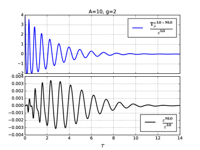
Figure 1: Parameters of the Wigner function (22): $A$=10, $\alpha_{0}=p_{0}=1$, $g$=2. Top panel: The trace of the energy-momentum tensor (54) normalised by LO energy density; bottom panel: the ration of the NLO energy density and the LO energy density

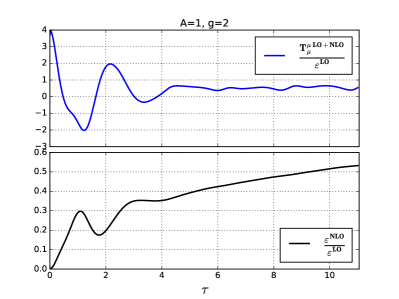
Figure 2: The same as for Fig.1 but with $A$=1

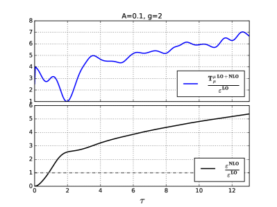
Figure 3: The same as for Fig.1 but with $A$=0.1

6 Conclusions

We calculated the quantum corrections to the trace of the energy-momentum tensor for the homogeneous $\varphi^{4}$ scalar field in two cases.

In the first case, the field placed inside a static box, we demonstrated that the NLO quantum corrections give contributions that vanish at large enough times. As one can see from lagrangian (1) the system posses the scale invariance which is broken by the initial conditions. However, during the time evolution the system forgets about initial state due to the self-interaction. That is why at the large times the scale invariance restores, $T_{\mu}^{\mu}=0$ and the quantum correction are negligible.

In the second case, the longitudinally expanding field, we claimed that the quantum correction might change the meanvalue of the trace of the energy-momentum tensor. In other words, the intermediate quasistationary regime characterised by the equation of state of the form different from the relativistic one $\varepsilon=3p$ is realised. This regime exists in the expanding geometry because the system transforms from the classical to the quantum one during the expansion. This phenomena occurs for the certain range of the parameters characterising the distribution of the initial conditions.

Note that the nonzero value of the trace of the energy-momentum tensor seen in Fig. (2) does not contradict with the scale invariance mentioned above. The scale invariance results in the requirement of $\langle T^{\mu}_{\mu}\rangle=0$ in equilibrium. However, the new regime we observed is an intermediate nonequilibrium one. Asymptotically, the system evolves to the equilibrium state with
$\varepsilon=0,\quad p=0$ due to expansion, hence scale invariance is restored.

In this work we describe the oversimplified scalar system. However, the phenomena we observed might be valuable for the description of the ultrarelativistic heavy-ion collisions as well. We suggest that similar quasistationary state can be formed due to nonequilibrium conditions, which are present in the matter created in such collisions.

Appendix A Quantum corrections to the CSA: scalar field theory

In this Appendix we describe a general formalism for calculation of quantum corrections to the Classical Statistical Approximation. For simplicity we consider the case of the scalar field, however, the idea can be extended to gauge fields as well. The main observation is that in the Keldysh-Schwinger formalism the CSA represents the Leading Order term of the semiclassical decomposition thus providing a basis for the systematic expansion.

Out of equilibrium an expectation value of observable $F(\hat{\varphi})$ at the moment $t_{1}$ can be calculated as a trace with density matrix as

$$\langle F(\hat{\varphi})\rangle_{t_{1}}=tr(F(\hat{\varphi})\hat{\rho}(t_{1}))\\ =\int\mathfrak{D}\xi(\vec{x})\ F(\xi)\langle\xi|\hat{U}(t_{1},t_{0})\hat{\rho}(t_{0})\hat{U}(t_{0},t_{1})|\xi\rangle,$$ (56)

where evolution of the density matrix $\hat{\rho}(t)$ is governed by the evolution operator $\hat{U}(t,t_{0})$

$$\hat{\rho}(t)=\hat{U}(t,t_{0})\hat{\rho}(t_{0})\hat{U}(t_{0},t),$$ (57)

$|\xi\rangle$ is an eigenstate of the field operator $\hat{\varphi}(\vec{x})|\xi\rangle=\xi(\vec{x})|\xi\rangle$ and $\int\mathfrak{D}\xi(\vec{x})$ is a path integral over all possible functions $\xi(\vec{x})$ originating from unity operator $\hat{1}=\int\mathfrak{D}\xi(\vec{x})\ |\xi\rangle\langle\xi|$.

After the usual procedure of the unity operator insertion we obtain the matrix elements of the evolution operator which path-integral representation is

$$\langle\xi|\hat{U}(t_{1},t_{0})|\xi_{1}\rangle=\int\limits_{\eta_{F}(t_{0},\vec{x})=\xi_{1}(\vec{x})}^{\eta_{F}(t_{1},\vec{x})=\xi(\vec{x})}\operatorname{{\mathcal{D}}}\eta_{F}(t,\vec{x})e^{iS[\eta_{F}]},$$

$$\langle\xi_{2}|\hat{U}(t_{0},t_{1})|\xi\rangle=\int\limits_{\eta_{B}(t_{0},\vec{x})=\xi_{2}(\vec{x})}^{\eta_{B}(t_{1},\vec{x})=\xi(\vec{x})}\operatorname{{\mathcal{D}}}\eta_{B}(t,\vec{x})e^{-iS[\eta_{B}]}.$$

Here $\eta_{F}(t,\vec{x})$ and $\eta_{B}(t,\vec{x})$ are the fields that lie on the forward ($\eta_{F}$) and backward ($\eta_{B}$) sides of the Keldysh contour (see LR1 for details). Thus the observable (56) reads

$$\langle F(\hat{\varphi})\rangle_{t_{1}}=D[\xi_{1},\rho_{0},\xi_{2}]\int\mathfrak{D}\xi\ F(\xi)\ \times$$ (58)

$$\int\limits_{\eta_{F}(t_{0},\vec{x})=\xi_{1}(\vec{x})}^{\eta_{F}(t_{1},\vec{x})=\xi(\vec{x})}\operatorname{{\mathcal{D}}}\eta_{F}(t,\vec{x})\int\limits_{\eta_{B}(t_{0},\vec{x})=\xi_{2}(\vec{x})}^{\eta_{B}(t_{1},\vec{x})=\xi(\vec{x})}\operatorname{{\mathcal{D}}}\eta_{B}(t,\vec{x})\ e^{iS_{K}[\eta_{F},\eta_{B}]}$$

where integration over initial configuration and the Keldysh action are

$$D[\xi_{1},\rho_{0},\xi_{2}]=\int\mathfrak{D}\xi_{1}\int\mathfrak{D}\xi_{2}\ \langle\xi_{1}|\hat{\rho}(t_{0})|\xi_{2}\rangle,$$

$$S_{K}[\eta_{F},\eta_{B}]=S[\eta_{F}]-S[\eta_{B}].$$

The final point of the trajectories which we integrate over is the time of observation $t_{1}$. However, it is convenient to extend the Keldysh contour to infinity so that the $t_{1}$ remains only in the observable $F$. The semiclassical decomposition is more evident with the following change of variables (often called the Keldysh rotation)

$$\phi_{c}=\frac{\eta_{F}+\eta_{B}}{2},\qquad\phi_{q}=\eta_{F}-\eta_{B}.$$ (59)

Then general expression for the observable reads

$$\langle F(\hat{\varphi})\rangle_{t_{1}}=D[\xi_{1},\rho_{0},\xi_{2}]\int\mathfrak{D}\chi\int\limits_{\phi_{c}(t_{0},\vec{x})=\frac{\xi_{1}(\vec{x})+\xi_{2}(\vec{x})}{2}}^{\phi_{c}(\infty,\vec{x})=\chi(\vec{x})}\operatorname{{\mathcal{D}}}\phi_{c}$$

$$\times\int\limits_{\phi_{q}(t_{0},\vec{x})=\xi_{1}(\vec{x})-\xi_{2}(\vec{x})}^{\phi_{q}(\infty,\vec{x})=0}\operatorname{{\mathcal{D}}}\phi_{q}\ F(\phi_{c}(t_{1}))\ e^{iS_{K}[\phi_{c},\phi_{q}]}.$$ (60)

This formula is rather general, hence we need to specify the Lagrangian. We use a scalar model with a quartic interaction term.

$$\operatorname{\mathcal{L}}=\frac{1}{2}\partial_{\mu}\varphi\partial^{\mu}\varphi-\frac{g^{2}}{4}\varphi^{4}+J\varphi,$$ (61)

$$S=\int d^{4}x\operatorname{\mathcal{L}}.$$

Here $J(t,\vec{x})$ is an auxiliary source which is kept to perform semiclassical decomposition. This source should be set to zero at the end of calculations.

For the Lagrangian (61) the Keldysh action (after integration by parts) reads

$$S_{K}[\phi_{c},\phi_{q}]=\int d^{3}x\ \dot{\phi}_{c}(t_{0},\vec{x})(\xi_{1}(\vec{x})-\xi_{2}(\vec{x}))$$

$$-\int d^{3}x\int\limits_{t_{0}}^{\infty}dt\ \Big{(}\phi_{q}A[\phi_{c}]-\frac{g^{2}}{4}\phi_{c}\phi_{q}^{3}\Big{)},$$ (62)

$$A[\phi_{c}]=[\partial_{\mu}\partial^{\mu}\phi_{c}+g^{2}\phi_{c}^{3}-J].$$ (63)

Note that the term $\phi_{q}A[\phi_{c}]=0$ corresponds to projecting onto the classical equation of motion for the Lagrangian (61).

The semiclassical approximation of (63) means expansion on $\phi_{q}$ around its saddle-point value

$$e^{i\frac{g^{2}}{4}\int\limits_{t_{0}}^{\infty}dt\int d^{3}x\ \phi_{c}\phi_{q}^{3}}=\underbrace{1}_{LO}+\underbrace{\frac{ig^{2}}{4}\int\limits_{t_{0}}^{\infty}dt\int d^{3}x\ \phi_{c}\phi_{q}^{3}}_{NLO}+....$$ (64)

This expansion does not require smallness of the coupling constant $g$. Practically, the Leading Order contribution contains quantum fluctuation up to one loop order.

The Leading Order contribution to observables corresponds to the first term in decomposition (64). The integration over $\phi_{q}$ and $\phi_{c}$ fields gives (see LR2 ; method for details)

$$\langle F(\hat{\varphi})\rangle_{t_{1}}=\\ =\int\mathfrak{D}\alpha(\vec{x})\mathfrak{D}p(\vec{x})f_{W}[\alpha(\vec{x}),p(\vec{x})),t_{0}]F(\phi_{cl}(t_{1},\vec{x})),$$ (65)

where

$$f_{W}[\alpha(\vec{x}),p(\vec{x}),t_{0}]=\int\mathfrak{D}\beta(\vec{x})\Big{\langle}\alpha+\frac{\beta}{2}\Big{|}\hat{\rho}(t_{0})\Big{|}\alpha-\frac{\beta}{2}\Big{\rangle}\\ \times\exp\Bigg{(}i\int d^{3}x\ p(\vec{x})\beta(\vec{x})\Bigg{)}.$$ (66)

is the Wigner functional defining initial state of the system, $\phi_{cl}$ is the solution of classical equation of motion

$$\partial_{\mu}\partial^{\mu}\phi_{cl}+g^{2}\phi_{cl}^{3}=J\Big{|}_{J=0}=0$$ (67)

with initial conditions given by

$$\phi_{cl}(t_{0},\vec{x})=\alpha(\vec{x}),\quad\dot{\phi}_{cl}(t_{0},\vec{x})=p(\vec{x})$$ (68)

and at zero axillary source $J(t,\vec{x})$.

Let us introduce new notation for averaging over initial conditions

$$\langle\mathcal{O}\rangle_{i.c.}=\int\mathfrak{D}\alpha(\vec{x})\mathfrak{D}p(\vec{x})f_{W}[\alpha(\vec{x}),p(\vec{x})),t_{0}]\ \mathcal{O}.$$ (69)

Then we can rewrite (65) shorter as

$$\langle F(\hat{\varphi})\rangle_{t_{1}}^{LO}=\langle F(\phi_{cl}(t_{1},\vec{x}))\rangle_{i.c.}.$$ (70)

The Next-to-Leading Order of the semiclassical decomposition (or quantum corrections to the CSA) is calculated as the second term of the expansion (64). The path integration over $\phi_{q}$ can not be done as easy as at LO level because of the additional $\phi_{q}^{3}$ part. However, each $\phi_{q}$ can be replaced by functional derivative over source $J$ due to $\phi_{q}J$ term in the Keldysh action (63) as

$$\frac{\delta}{\delta J(t,\vec{x})}e^{iS_{K}[\phi_{c},\phi_{q}]}=i\phi_{q}(t,\vec{x})e^{iS_{K}[\phi_{c},\phi_{q}]}.$$ (71)

This observation allows to perform functional integration over $\phi_{q}$ and $\phi_{c}$ to obtain the answer for expectation value of the observable up to NLO level

$$\langle F(\hat{\varphi})\rangle_{t_{1}}^{LO+NLO}=\Bigg{\langle}F(\phi_{cl}(t_{1},\vec{x}))$$ (72)

$$+\frac{g^{2}}{4}\int\limits_{t_{0}}^{t_{1}}dt_{2}\int d^{3}x_{2}\phi_{cl}(t_{2},\vec{x}_{2})\frac{\delta^{3}F(\phi_{cl}(t_{1},\vec{x}))}{\delta J^{3}(t_{2},\vec{x}_{2})}\Bigg{|}_{J=0}\Bigg{\rangle}_{i.c.}.$$

The expression above shows that there is no necessity in any new information for evaluation of the NLO correction. One should find the classical trajectory as a function of the initial conditions, perform three variations over auxiliary source, integrate over intermediate time and average with the Wigner functional. It is easy to recast all terms of the semiclassical approximation to the following general form

$$\langle F(\hat{\varphi})\rangle_{t_{1}}=$$ (73)

$$=\Bigg{\langle}\bar{T}e^{\frac{g^{2}}{4}\displaystyle\int d\tau d\vec{y}\ \phi_{cl}(\tau,\vec{y})\frac{\delta^{3}}{\delta J^{3}(\tau,\vec{y})}}\ F(\phi_{cl}(t_{1},\vec{x}))\Bigg{\rangle}_{i.c.}$$

Here $\bar{T}$ denote the anti-time ordering which is required to recover exponential form. The formula (73) shows that the building block of the semiclassical decomposition is the full nonperturbative solution of the classical EoM $\phi_{cl}$ rather than the Green’s function of the perturbative approach. Hence, the strong field limit can be considered with the semiclassical method, however, only for the narrow range of problems allowing the semiclassical decomposition itself.

Numerical calculations can be slightly simplified. Let us define $k$-th variation of the classical solution over source $J$ as

$$\frac{\delta^{k}\phi_{cl}(x_{1})}{\delta J^{k}(x_{2})}=\Phi_{k}(x_{1};x_{2}).$$ (74)

Then

$$\frac{\delta^{3}F(\phi_{cl}(x_{1}))}{\delta J^{3}(x_{2})}=\frac{\partial F}{\partial\phi_{cl}}\Phi_{3}(x_{1};x_{2})+\frac{\partial^{3}F}{\partial\phi_{cl}^{3}}\Phi_{1}^{3}(x_{1};x_{2})\\ +3\frac{\partial^{2}F}{\partial\phi_{cl}^{2}}\Phi_{1}(x_{1};x_{2})\Phi_{2}(x_{1};x_{2}).$$ (75)

Functions $\Phi_{k}(x_{1};x_{2})$ can be found by variation of the classical EoM.

$$\frac{\delta^{3}}{\delta J^{3}(x_{2})}\left(\partial_{\mu}\partial^{\mu}\phi_{cl}(x_{1})+g^{2}\phi_{cl}^{3}(x_{1})=J(x_{1})\right).$$

Hence, to calculate the quantum correction to the CSA one need to find the solution of four linked differential equations

$$\partial_{\mu}\partial^{\mu}\phi_{cl}(x_{1})+g^{2}\phi_{cl}^{3}(x_{1})=0,$$

$$L_{t_{1}}\Phi_{1}(x_{1};x_{2})=\delta^{(4)}(x_{1}-x_{2}),$$

$$L_{t_{1}}\Phi_{2}(x_{1};x_{2})=-6g^{2}\phi_{cl}(x_{1})\Phi_{1}^{2}(x_{1};x_{2}),$$

$$L_{t_{1}}\Phi_{3}(x_{1};x_{2})=-6g^{2}\Phi_{1}^{3}(x_{1};x_{2})$$

$$-18g^{2}\phi_{cl}(x_{1})\Phi_{1}(x_{1};x_{2})\Phi_{2}(x_{1};x_{2})$$

$$L_{t_{1}}=\partial^{2}_{t_{1}}-\partial^{2}_{\vec{x}_{1}}+3g^{2}\phi_{cl}^{2}(x_{1}).$$ (76)

without knowledge of the exact dependence of the classical solution $\phi_{cl}(x)$ of auxiliary source $J(x)$.

References

(1)
F. Gelis, Int.J.Mod.Phys. E24 (2015), 1530008
(2)
A. Kurkela, Nucl.Phys. A956 (2016) 136-143
(3)
J. Berges, Nonequilibrium Quantum Fields: From Cold Atoms to Cosmology, arXiv:1503.02907
(4) J. Berges and T. Gasenzer, Phys. Rev. A 76, 033604 (2007)
(5) Kean Loon Lee, Nick P. Proukakis, arXiv:1607.06939 [cond-mat.quant-gas]
(6) D. T. Son, hep-ph/9601377.
(7) S. Y. Khlebnikov and I. I. Tkachev, Phys. Rev. Lett. 77, 219 (1996)
(8) D. Boyanovsky, Phys. Rev. D 92, 023527 (2015)
(9)
T. Lappi, L. McLerran, Nucl.Phys. A772 (2006) 200-212
(10)
P. Romatschke, R. Venugopalan, Phys.Rev. D74 (2006) 045011
(11)S. Mrowczynski, B. Muller Phys. Rev. D50, 7542-7552 (1994)
(12)K. Fukushima, F. Gelis, L. McLerran, Nucl.Phys.A786 (2007) 107-130
(13) K. Dusling, T. Epelbaum, F. Gelis, R. Venugopalan, Nucl.Phys. A850 (2011) 69-109
(14) T. Epelbaum, F. Gelis, Nucl.Phys. A872 (2011) 210-244
(15) K. Dusling, T. Epelbaum, F. Gelis, R. Venugopalan, Phys.Rev. D86 (2012) 085040
(16) A.V. Leonidov, A.A. Radovskaya, JETP Lett. 101 (2015), 215
(19) Julian S. Schwinger , J.Math.Phys. 2 (1961) 407-432
(20) H. Lee, M.O. Scully, Journal of Chemical Physics 73, 2238 (1980)
(21) L.Bonnet, Journal of Chemical Physics 139, 114108 (2013)
(22) Yu. Kovchegov, B. Wu, Time-dependent observables in heavy ion collisions. Part I. Setting up the formalism, JHEP 03 (2018), 158
(23) Yu. Kovchegov, B. Wu, Time-dependent observables in heavy ion collisions. Part II. In search of pressure isotropization in the
theory, JHEP 03 (2018), 157
(24) T. Epelbaum, F. Gelis, B. Wu, Phys.Rev. D90 (2014), 065029
(25)J. Berges, T. Gasenzer, Phys.Rev. A76 (2007) 033604
(26)
J. Jalilian-Marian, A. Kovner, A. Leonidov, H. Weigert, Phys. Rev. D 59 (1998) 014014
(27)
E. Iancu, A. Leonidov, L. D. McLerran, Nucl. Phys. A 692 (2001) 583
(28)
E. Ferreiro, E. Iancu, A. Leonidov, L. McLerran, Nucl. Phys. A 703 (2002) 489
(29)
E. Iancu, A. Leonidov, L. D. McLerran, Phys. Lett. B 510 (2001) 133
(30)
S. Jeon, Annals Phys. 340 (2014) 119-170
(31)A. Kovner, M. Lublinsky, Y. Mulian, Phys.Rev. D89 (2014), 061704