11email: daria.kubyshkina@oeaw.ac.at 22institutetext: Institute of Computational Modelling of the Siberian Branch of the Russian Academy of Sciences, 660036 Krasnoyarsk, Russian Federation 33institutetext: Siberian Federal University, 660041, Krasnoyarsk, Russian Federation 44institutetext: Institute for Astronomy, University of Vienna, Türkenschanzstrasse 17, A-1180 Vienna, Austria 55institutetext: Institute of Physics/IGAM, University of Graz, Universitätsplatz 5, A-8010 Graz, Austria
A grid of upper atmosphere models for 1–40 planets: application to CoRoT-7 b and HD219134 b,c
There is growing observational and theoretical evidence suggesting that atmospheric escape is a key driver of planetary evolution. Commonly, planetary evolution models employ simple analytic formulae (e.g., energy limited escape) that are often inaccurate, and more detailed physical models of atmospheric loss usually only give snapshots of an atmosphere’s structure and are difficult to use for evolutionary studies. To overcome this problem, we upgrade and employ an already existing upper atmosphere hydrodynamic code to produce a large grid of about 7000 models covering planets with masses 1 – 39 with hydrogen-dominated atmospheres and orbiting late-type stars. The modelled planets have equilibrium temperatures ranging between 300 and 2000 K. For each considered stellar mass, we account for three different values of the high-energy stellar flux (i.e., low, moderate, and high activity). For each computed model, we derive the atmospheric temperature, number density, bulk velocity, X-ray and EUV (XUV) volume heating rates, and abundance of the considered species as a function of distance from the planetary center. From these quantities, we estimate the positions of the maximum dissociation and ionisation, the mass-loss rate, and the effective radius of the XUV absorption. We show that our results are in good agreement with previously published studies employing similar codes. We further present an interpolation routine capable to extract the modelling output parameters for any planet lying within the grid boundaries. We use the grid to identify the connection between the system parameters and the resulting atmospheric properties. We finally apply the grid and the interpolation routine to estimate atmospheric evolutionary tracks for the close-in, high-density planets CoRoT-7 b and HD219134 b,c. Assuming the planets ever accreted primary, hydrogen-dominated atmospheres, we find that the three planets must have lost them within a few Myr.
Key Words.:
Hydrodynamics – Planets and satellites: atmospheres – Planets and satellites: physical evolution – Planets and satellites: individual: CoRoT-7 b, HD219134 b, HD219134 c1 Introduction
The results of the NASA Kepler mission have revealed the presence of a large variety of planetary systems, with structures and geometries often very different from the Solar System. The detection of a large number of extra-solar planets (hereafter exoplanets) with masses and radii in between those of Earth and Neptune is a striking example (e.g., Bonfils et al. 2013; Mullally et al. 2015).
Super-Earths and mini-Neptunes, absent in the Solar System, are extremely common and are easier to detect and characterise compared to Earth-mass planets. Therefore, these planets are raising great interest and are among the primary targets for planet-finding and -characterisation missions such as CHEOPS (Broeg et al. 2013), TESS (Ricker et al. 2015), CUTE (Fleming et al. 2018), JWST (Gardner et al. 2006; Deming et al. 2009), PLATO (Rauer et al. 2014), and ARIEL (Tinetti et al. 2017).
Super-Earths and mini-Neptunes can have a large variety of average densities ranging from being consistent with rocky planets up to planets with thick hydrogen-dominated envelopes (e.g., Weiss & Marcy 2014; Lopez & Fortney 2014; Howe et al. 2014; Wolfgang et al. 2016; Cubillos et al. 2017a). Assuming planets were formed inside the protoplanetary disk, thus accreted a gaseous envelope, the rocky planets most likely lost their primordial hydrogen-rich envelope through escape, while the low-density planets still retain their primordial atmosphere. Fulton et al. (2017) revealed the presence of a dichotomy in the radius distribution of the super-Earths and mini-Neptunes discovered by the Kepler mission (see also Van Eylen et al. 2017; Fulton & Petigura 2018), which Owen & Wu (2017) and Jin & Mordasini (2017) interpreted as being the result of atmospheric escape processes occurring during the first few hundred million years following the dispersal of the protoplanetary disk (see Ginzburg et al. 2018, for an alternative explanation).
These works (see also e.g., Lundkvist et al. 2016) clearly showed that atmospheric escape is likely to play a major role in shaping the currently observed exoplanet population and mass-radius distribution. Atmospheric escape is gaining also more relevance in the characterisation of lower atmospheres: for example, Cubillos et al. (2017b) showed that the penetration depth in the planetary atmosphere of the high-energy stellar radiation (hereafter called XUV: EUV + X-ray) can be used to constrain the lower pressure levels for the presence of clouds.
In this study, we focus on 1–40 planets that have accreted a primordial hydrogen-dominated envelope while forming inside the protoplanetary nebula (see e.g., Stökl et al. 2016). Once released from the protoplanetary nebula, planets experience a short phase of extreme hydrodynamical thermal escape, caused mostly by their high temperature and low gravity (Stökl et al. 2015; Owen & Wu 2016; Ginzburg et al. 2016; Fossati et al. 2017). This so-called “boil-off” phase is followed by a much longer one in which the hydrodynamic atmospheric escape is driven by the incident stellar XUV flux (e.g., Lammer et al. 2003). Usually, this type of escape is called “blow-off” and the atmospheric escape rates can be estimated using the energy- or recombination-limited formulas (Watson et al. 1981; Lecavelier des Etangs et al. 2004; Erkaev et al. 2007; Lammer et al. 2009; Ehrenreich and Désert 2011; Salz et al. 2016; Chen & Rogers 2016). Both these escape conditions are different from classical Jeans escape, in which only the fraction of particles lying close to or above the exobase with velocities larger than the planetary escape velocity leave the planet.
Overall, the energy-limited formula reproduces well the escape rates obtained through detailed hydrodynamic upper atmosphere modelling, particularly for close-in gas giants with atmospheres in blow-off (e.g., Lammer et al. 2009; Fossati et al. 2015; Salz et al. 2016; Erkaev et al. 2016, 2017). Because of its analytical form, hence allowing for fast computations, the vast majority of planetary evolution and population synthesis models employ the energy- and recombination-limited formalisms to model atmospheric escape for a wide range of planets subject to (very) different stellar irradiation levels (e.g., Jackson et al. 2012; Batygin & Stevenson 2013; Jin et al. 2014; Lopez & Fortney 2013; Owen & Wu 2017; Jin & Mordasini 2017; Lopez 2017). However, it has also been shown that in many cases, particularly for highly irradiated low-mass planets and for planets with hydrostatic atmospheres, the energy-limited formula tends to significantly over- or under-estimate the escape rates (e.g., Lammer et al. 2016; Erkaev et al. 2015, 2016; Salz et al. 2016; Owen & Mohanty 2016; Fossati et al. 2017, 2018).
In this work, we follow and expand on the approach of Johnstone et al. (2015), who computed a small grid of upper atmosphere hydrodynamic models and extracted the mass-loss rates by interpolating between the grid cells to model the possible evolution of the atmosphere of early-Earth and to avoid the assumptions connected with the use of analytical formalisms. This approach enables more reliable planetary evolution computations, appropriately accounting for boil-off, blow-off, and Jeans escape, and smoothly transitioning among the different escape regimes, without significantly affecting the computational time.
We present here a large grid of upper atmosphere hydrodynamic models computed for a wide range of parameters for 1–40 planets. We present also an interpolation routine we developed to extract model output parameters, such as atmospheric temperatures, velocities, densities and hydrogen species abundances, and resulting escape rates, for any planet contained within the grid boundaries. The model grid and interpolation routine can quickly produce the results of a full hydrodynamic upper atmosphere computation for planets covered by the grid, without the need to actually run a model. This enables faster, yet more accurate, interpretation and characterisation of planetary atmospheres in comparison to the results provided by, for example, the energy-limited formula. This has now become particularly important to understand the mass-radius-period distribution of the large number of planets expected to be discovered in the near future by all-sky surveys such as TESS and PLATO (Rauer et al. 2014; Barclay et al. 2018). Furthermore, a grid approach enables accurate planetary evolution and population synthesis computations and the thorough exploration of trends in the characteristics of planetary upper atmospheres as a function of system parameters.
This paper is organised as follows. In Section 2, we present the hydrodynamic model used to compute the grid and a comparison to the literature, while in Section 3 we describe the grid boundaries and structure. Section 4 gives an overview of the results and provides a description of the interpolation routine. Section 5 discusses the results and presents an application of the grid to the case of the low-mass, close-in planets CoRoT-7 b and HD219134 b,c. In Section 6, we gather our conclusions.
2 Upper atmosphere modelling
2.1 The hydrodynamical model
The construction of a large grid requires a hydrodynamic model satisfying two basic criteria: it has to reliably compute upper atmosphere profiles within a short time and it has to be able to cover a wide range of stellar, orbital, and planetary parameters. The first point is critical because the need to cover a large parameter space requires the computation of numerous models (i.e., 1000). These criteria are well matched by the one-dimensional hydrodynamic upper atmosphere model described by Erkaev et al. (2016), which has been successfully tested for a very wide range of planetary systems (e.g., Lammer et al. 2013, 2016; Erkaev et al. 2013, 2014, 2015, 2016, 2017; Fossati et al. 2017; Cubillos et al. 2017a, b).
To simplify and speed up the calculation of a large number of models in the grid, we have implemented a new computational scheme, which provides an automatic selection of an initial atmospheric profile for each planet (i.e., each point in the grid). Our hydrodynamic code includes X-ray heating and cooling, which are relevant for some of the planets close to our grid boundaries. The addition of X-ray heating provides us also with a further important degree of freedom relevant for young, close-in planets, which are subject to strong blow-off (e.g., Kubyshkina et al. 2018). We provide below a detailed description of the modelling scheme.
We set the lower boundary of the atmospheric profile at the photospheric radius (), where we considered the planetary atmosphere to have a temperature equal to the equilibrium temperature (; see Fossati et al. 2017) assuming zero Bond albedo and full energy redistribution. The upper boundary was set at the Roche radius
| (1) |
where and are the planetary and stellar masses, respectively, and is the orbital separation. The boundary conditions at the upper limit were set to be free, that is the position at which the radial derivatives of the computed quantities become zero. We assume a pure hydrogen atmosphere and that at the lower boundary the atmosphere is composed exclusively of molecular hydrogen. Following Fossati et al. (2017), for each planet we compute the pressure at the lower boundary of the atmosphere assuming solar abundances.
The chemical network implemented in the code accounts for hydrogen dissociation, recombination, and ionisation. In addition, the code accounts for Ly cooling, XUV heating, and cooling. In the literature, the height averaged heating efficiency (), which is the fraction of absorbed stellar XUV radiation converted into thermal energy of the atmosphere, ranges between 10% and 60% (e.g., Watson et al. 1981; Yelle 2004; Murray-Clay et al. 2009; Cecchi-Pestellini et al. 2009; Owen & Jackson 2012; Shematovich et al. 2014; Salz et al. 2016). Salz et al. (2016) showed that for Earth- to Jupiter-mass planets varies approximately between 10% and 25%. The implementation of a self-consistent calculation of the heating efficiency would have made the hydrodynamic code too slow to allow the computation of a large grid. For this reason, we decided to follow the considerations of Erkaev et al. (2016) adopting for all planets a constant value of 15% at all wavelengths.
The code solves the equations for mass, momentum, and energy conservation
| (2) | |||||
| (3) | |||||
| (4) |
where , , and are the mass density, bulk velocity, and temperature as a functions of the radial distance from the planetary center , respectively. The quantity
| (5) |
is the planetary gravitational potential accounting for the Roche lobe effect (Erkaev et al. 2007). In Equation (5), , , (where is the orbital separation), and . The term
| (6) |
in erg cm-1 s-1, is the thermal conductivity of the neutral gas (Watson et al. 1981). We do not account for the thermal conductivity of electrons and ions. We tested this assumption concluding that the inclusion of this effect leads to negligible variations to the results. In particular, the largest effect is on the temperature maximum for highly irradiated, high-density planets, which decreases by as much as , with a typical decrease lying around .
The terms and are the atmospheric pressure and thermal energy, which are defined as
| (7) |
and
| (8) |
Finally, , , and are the volume heating/cooling rates for XUV heating, cooling, and cooling, respectively.
The spectral dependence of the stellar XUV flux varies significantly from star to star. Since we aim at computing a grid of models valid for a wide range of system parameters, it is impossible to account for the full spectral dependence of the stellar XUV flux, though the code would in principle allow it. For this reason, we assumed that the whole stellar EUV flux is emitted at a single wavelength of 60 nm (Murray-Clay et al. 2009). To account for X-ray heating, we assumed that the stellar X-ray photons are all emitted at a wavelength of 5 nm, roughly in the middle of the X-ray wavelength band.
The XUV heating function is therefore composed of two terms, and , which describe the heating by the EUV and X-ray stellar flux, respectively. These two functions are constructed in the same way, except for the absorption cross-sections and absorption functions of the stellar flux inside the planetary atmosphere that are defined at 5 and 60 nm. The total heating function thus becomes = . Each heating function takes the form of
| (9) |
where stands for either EUV or X, is the absorption cross-section for the specific wavelength, and is the flux absorption function
| (10) |
In Equation (10), is a function in spherical coordinates describing the spatial variation of the EUV, or X-ray, flux due to atmospheric absorption (Erkaev et al. 2015) and , in this case, corresponds to the radial distance from the planetary center.
We defined the absorption cross-section as , where , = 13.6 eV is the hydrogen ionisation energy, and is the photon energy in a specific wavelength range ( = 20 eV in the EUV and 248 eV in the X-ray domain). It follows that the EUV flux absorption cross-sections are cm-3 and cm-3 for atomic and molecular hydrogen, respectively (Spitzer 1978). The X-ray absorption cross-section is approximately three orders of magnitude smaller than the EUV one. This implies that the stellar X-ray photons penetrate deeper into the planetary atmosphere than the EUV photons, thus heating the atmosphere closer to . For this reason, despite that stellar X-ray fluxes are significantly smaller than the EUV fluxes, X-rays can still cause significant atmospheric heating.
We implemented Ly cooling by adding the following function to the energy conservation equation (Watson et al. 1981)
| (11) |
To implement cooling, we followed Miller et al. (2013) and added in the energy conservation equation the function
| (12) |
where are the temperature-dependent coefficients listed in Table 5 of Miller et al. (2013). Heating rates in 9, 11 and 12 are given in erg cm-3 s-1.
Since we consider non-magnetic planets, we did not include electric conduction due to ionised components. If large enough, conduction prevents the penetration of the interplanetary magnetic field inside the ionosphere, which results in the formation of a magneto pause separating the stellar wind protons from the atmospheric ions. In addition, in case of a strongly magnetised planet, the hydrodynamic flow of the escaping ionised gas can produce electric currents in the ionosphere, which would generate a resisting force against the escaping hydrodynamic flow.
The complete list of chemical reactions and the relative cross-sections (, , , , , , , , , ) considered in the model are listed in Appendix A. The continuity equations connected with the chemical reactions are
| (13) | |||||
| (14) | |||||
| (15) | |||||
| (16) |
Here, the electron density is defined as
| (17) |
while the total hydrogen number density is the sum of the number density of all species. Finally, the mass density is
| (18) |
2.2 Comparison with previous results
To test the modelling results, we compared the mass-loss rates obtained for a sample of previously (observationally and/or theoretically) studied planets with those present in the literature (Table 1). Of the four planets considered in this comparison, just GJ 436 b and Kepler-11 b fall within the grid boundaries and the inclusion in the comparison of the two classical hot Jupiters, HD209458 b and HD189733 b, is due to the fact that these are the best studied systems in terms of atmospheric escape. For our calculations, we employed the stellar XUV fluxes and masses given by Guo & Ben-Jaffel (2016).
| ID | |||||||
| [AU] | [] | [] | [] | [] | [] | ||
| HD209458 b | 90 | 0.047 | 1086 | 1.148 | 1.2 | 8.0 | 3.3 (a) |
| (b) | |||||||
| (c) | |||||||
| GJ 436 b | 58 | 0.02887 | 1760 | 0.452 | 3.95 | 2.9 | 1 (d) |
| 1 (e) | |||||||
| 2.2 (f) | |||||||
| 4.5 (c) | |||||||
| Kepler-11 b | 18 | 0.091 | 278 | 0.95 | 1.1 | 7.5 | (g) |
| (h) | |||||||
| (e) | |||||||
| HD189733 b | 179 | 0.03 | 24778 | 0.8 | 4.9 | (b) | |
| (e) | |||||||
| (c) |
We find good agreement between our values and those published in the literature, in particular for HD209458 b, GJ 436 b, and Kepler-11 b. Note that for Kepler-11 b Kislyakova et al. (2014) considered mostly non-thermal escape, which is significantly smaller than the XUV driven escape, while Lammer et al. (2013) adopted a completely different lower boundary condition, which led to a significant underestimation of the mass-loss rates (see Lammer et al. 2016, for more details). In case of HD189733 b, our estimation lies within the interval given by Bourrier & Lecavelier des Etangs (2013), but significantly below that of Guo & Ben-Jaffel (2016), (which appears to be an outlier compared to other estimations), and it is an order of magnitude smaller than that given by the energy-limited formula. The reason may be that Equation (11) possibly overestimates the cooling for hot Jupiters, which are optically thick to L in the region where the cooling peaks, so the radiation does not escape efficiently. This was addressed in detail by Menager et al. (2013) and Koskinen et al. (2013).
3 Model grid
We designed the grid to model super-Earths and mini-Neptunes orbiting main-sequence stars. The computations were made considering the following system parameters: planetary mass , planetary radius , equilibrium temperature , orbital separation d0, stellar mass , and the stellar XUV flux at the planetary orbit . As mentioned above, we consider the planetary radius to be equal to the photospheric radius assuming a clear hydrogen-dominated atmosphere and solar abundances.
The stellar temperature and radius change along the main-sequence phase of evolution, defined as in Yi et al. (2001). Consequently, each value corresponds to a range of possible orbital separations defined by the possible range of changes in stellar parameters. By fixing stellar equilibrium temperature and radius, this range of orbital separations corresponds to variations of the order of 10–20 K. To save computation time, we adopted one value of the orbital separation, namely that at the center of the range, for each value. Therefore, d0 is derived from the stellar mass and equilibrium temperature. This implies that just five input parameters of the grid are independent.
We computed models for planets with masses ranging between 1 and 39 (i.e., up to twice the mass of Neptune or one tenth of Jupiter’s), with a variable step size that increases logarithmically with mass for a total of 14 planetary mass values. The planetary radius ranges between 1 and 10 (i.e., up to one Jupiter radius and 2.5 times Neptune’s), in regular steps of 1 (i.e., total of 10 planetary radius values). The equilibrium temperature of the planets in the grid ranges between 300 and 2000 K with regular steps of 400 K (i.e., total of 5 temperature values). The cooler boundary was set to cover planets orbiting in the habitable zone, while the hotter boundary was set to ensure that our assumption on the composition of the atmosphere at the lower boundary (i.e., H2-dominated) holds (Koskinen et al. 2010). Our focus is on planets orbiting early M- to late F-type stars, thus we considered stellar masses between 0.4 and 1.3 for a total of five different stellar masses. We plan to extend the grid to lower mass stars, which are primary targets for various planet-finding facilities, such as CARMENES (Quirrenbach et al. 2010) and TESS (Ricker et al. 2015). Table 2 lists the values of stellar mass, equilibrium temperature, planetary radius, and planetary mass considered for the computation of the grid.
| K | |||
|---|---|---|---|
| 0.4 | 300 | 1.0 | 1.0 |
| 0.6 | 700 | 2.0 | 1.6 |
| 0.8 | 1100 | 3.0 | 2.1 |
| 1.0 | 1500 | 4.0 | 3.2 |
| 1.3 | 2000 | 5.0 | 4.3 |
| 6.0 | 5.0 | ||
| 7.0 | 6.7 | ||
| 8.0 | 7.8 | ||
| 9.0 | 9.0 | ||
| 10.0 | 12.1 | ||
| 16.2 | |||
| 21.7 | |||
| 29.1 | |||
| 39.0 |
We set the range of orbital separations covered by the grid on the basis of the stellar mass and planetary equilibrium temperature, thus stellar radius () and effective temperature (). The two last quantities were derived considering the range of radii and effective temperatures covered by a star of each considered mass along the main-sequence on the basis of stellar evolutionary tracks (Yi et al. 2001). This leads to the fact that only a limited range of orbital separations had to be considered for each given stellar mass, saving computation time. Considering all stellar masses, the orbital separation ranges between 0.002 and 1.3 AU.
For the XUV stellar fluxes, we considered three distinct values corresponding roughly to a chromospherically active star, a moderately active star, and a quiet star. To set the high XUV flux value, we considered that the X-ray saturation threshold observed for main-sequence late-type stars lies at roughly , where is the X-ray luminosity, is the bolometric luminosity at the zero age main sequence (Yi et al. 2001), and ranges between 2.5 (e.g., Reiners et al. 2014) and 3.1 (e.g., Wright et al. 2011). We therefore set the maximum X-ray luminosity as and the minimum X-ray luminosity as . The EUV stellar luminosity was then derived from the X-ray luminosity following (Sanz-Forcada et al. 2011)
| (19) |
The specific X-ray and EUV luminosities adopted for each stellar mass are listed in Table 3.
| [ erg s-1] | [ erg s-1] | [ erg s-1] | [ erg s-1] | [ erg s-1] | [ erg s-1] | [ erg s-1] | |
|---|---|---|---|---|---|---|---|
| 0.4 | |||||||
| 0.6 | |||||||
| 0.8 | |||||||
| 1.0 | |||||||
| 1.3 |
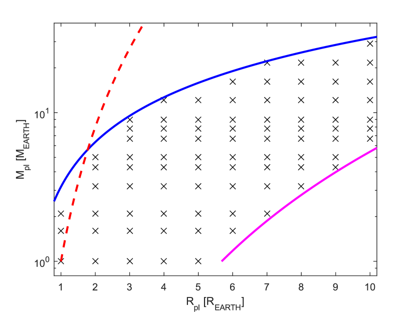
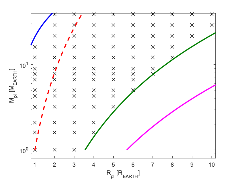
To avoid spending time calculating planets that probably do not exist in nature, we restricted the computations to planets with an average density larger than 0.03 g cm-3 (equal to the lowest known measured density Masuda 2014) and a restricted Jeans escape parameter smaller than 80 (where atmospheres are presumably stable), where (Jeans 1925; Chamberlain 1963; Öpik 1963; Fossati et al. 2017)
| (20) |
is the value of the Jeans escape parameter calculated at the observed planetary radius and mass for the planet’s equilibrium temperature and considering atomic hydrogen, independent of the atmospheric temperature profile. We further excluded planets where the Roche lobe is closer than 0.5 planetary radii from the surface. This cut is most relevant for the hottest planets ( 1500 K) orbiting stars less massive than about 0.8 . As an example, Figure 1 shows the positions of the modelled planets in the mass-radius diagram at two different equilibrium temperatures.
To summarise, our grid consists of five data points for stellar mass and planetary equilibrium temperature, each, ten data points for planetary radius, 14 data points for planetary mass, and three data points for stellar XUV luminosity. This leads to a total of 10 500 models. However, because of the restrictions described above, the total number of models in the grid reduces to 6 700.
4 Results
For each modelled planet, we computed the main atmospheric parameters as a function of the radial distance from the planetary center. These include the atmospheric temperature, number density, bulk velocity, X-ray and EUV volume heating rates, and abundance of the considered species (, H, , , , e). From these quantities, we estimated the positions of the maximum dissociation and ionisation (the distances corresponding to the maximum of the number densities of atomic and ionised hydrogen, respectively), the mass-loss rate , and the effective radius of the XUV absorption that is defined as
| (21) |
where is the XUV flux as it travels through the planetary atmosphere along the star-planet direction and is mostly determined by the density . The mass-loss rate is computed as the product of the atmospheric density and velocity at the upper boundary. To account for the fact that we employ a one dimensional model, this value is then multiplied by the surface area of a sphere with radius equal to . For most planets, hydrogen dissociation occurs in a relatively narrow range of distances, which is typically smaller than one planetary radius.
Although the atmospheric parameters vary significantly across the grid, there are some common characteristics. One of the most important ones is that the atmospheric behaviour strongly depends on . For planets with low values (i.e., 10), the atmosphere is weakly bound to the planet and experiences strong boil-off. The energy budget of these planets is determined by adiabatic cooling and the mass-loss rates are not significantly affected by variations in the stellar XUV flux. With increasing , the role of planetary gravity in the atmospheric dynamics decreases and the atmosphere gradually switches to being controlled by the stellar XUV heating. We find that the border between these two regimes lies at values ranging between 10 and 30, depending on the system parameters, in agreement with Fossati et al. (2017).
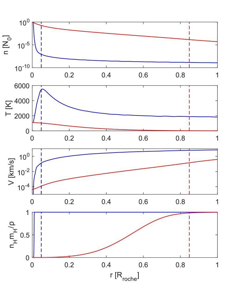
As an example, Figure 2 compares the atmospheric density, temperature, velocity, and atomic hydrogen abundance profiles for two planets with equal to 4.8 and 66.7. The two planets orbit a 1 star, have an equilibrium temperature of 1100 K (i.e., = 0.075 AU), a radius of 3 , and are subject to an incident XUV flux of 92.6 . The planet with the lower has a mass of 2.1 , while that with the higher has a mass of 29.1 . For the less massive planet, we derived a value of the effective XUV absorption radius () of 5.5 , a Roche radius of 6.5 , and a mass-loss rate of . For the more massive planet, we derived a value of 1.2 , a Roche radius of 17.1 , and a mass-loss rate of . For the less massive planet, we found also that the velocity of the atmospheric particles becomes supersonic close to the Roche radius (at 6.2 ), while for the more massive planet the particles become supersonic well below the upper boundary (at 9.1 ).
Figure 2 shows how the density decreases with increasing distance from the planetary surface; the decrease is steeper for the more massive planet, because it hosts a more compact atmosphere (because of stronger gravity). The temperature profiles show that the stellar XUV flux efficiently heats the more massive planet inducing a temperature peak at the thermospheric level, reaching its maximum close to , where the model indicates also the presence of strong dissociation. At higher altitudes, the atmosphere is composed fully of atomic hydrogen and is dominated by adiabatic cooling, which is caused by the atmosphere’s expansion and dominates over XUV heating. In contrast, for the less massive planet, the XUV stellar flux does not penetrate deep enough into the planetary atmosphere to cause thermospheric heating, thus the atmosphere expands adiabatically, driven by its internal heat and by the low planetary gravity. In general, the profiles of planets with low values do not develop steep gradients (see e.g., Kubyshkina et al. 2018), making the definition of and of the position of the maximum dissociation and ionisation ambiguous. We will come back to this point in Section 5.1.2.
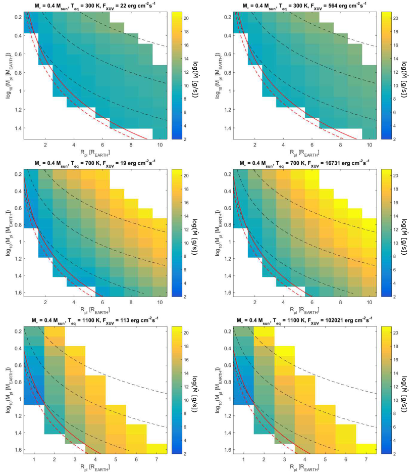
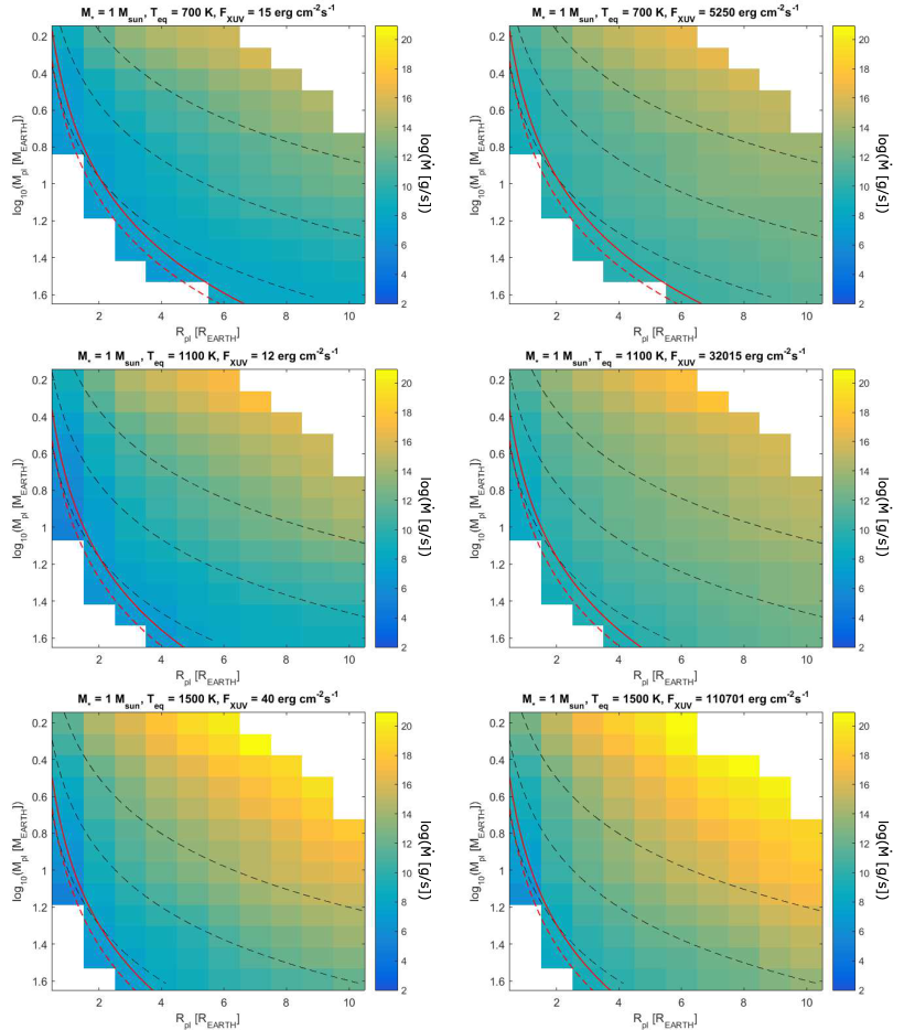
Because of its relevance, e.g., in understanding planetary evolution, the mass-loss rate is one of the key output parameters of the modelling. Figure 3 shows a few examples of how the mass-loss rates depend on planetary mass and radius for different and values. All planets shown in Figure 3 orbit a 1.0 star. Appendix C presents similar plots, but for planets orbiting stars more/less massive than 1.0 . As expected, the highest mass-loss rates are found for the lowest gravity planets, whose atmospheres are in boil-off. With increasing (thus gravity), the mass-loss rates decrease first steeply and then more gradually. The dependence of the mass-loss rates on the stellar XUV flux tends to strengthen with increasing planetary mass.
We further checked a posteriori the validity of the hydrodynamic equations to the modelled planets, namely whether the atmosphere remains collisional (i.e., with efficient energy redistribution) up to the sonic point. This condition is satisfied if the Knudsen number = 1, where is the mean free path of the gas and = is the characteristic length scale. In Figure 3 and in the Figures in Appendix C, we show lines corresponding to = 1 and = 10. This indicates that the results we obtained for the highest-density planets in our grid should be taken with caution. However, these are anyway planets for which the high bulk density disfavours the presence of a hydrogen-dominated atmosphere.
au au au
In Figure 4, we compare the mass-loss rates as a function of (top) and planetary mass (bottom) obtained from the hydrodynamic modelling with those derived from the energy-limited formula
| (22) |
where the factor accounts for Roche-lobe effects (Erkaev et al. 2007). By design, the energy-limited approximation works best for planets for which the atmosphere is hydrodynamic and the escape is driven by absorption of the stellar XUV flux, i.e., in blow-off. This implies that Equation (22) overestimates the mass-loss rates for planets with hydrostatic atmospheres (see e.g., Fossati et al. 2018). The top panel of Figure 4 shows that, being in boil-off, the mass-loss rates for the lower-gravity planets are much higher than those predicted by Equation (22). We also find that the / ratio decreases steeply with increasing , having all other parameters constant. The value of at which the mass-loss rate computed with the hydrodynamic code becomes comparable to is about 20, in agreement with Owen & Wu (2016) and Fossati et al. (2017). Figure 4 shows also that Equation (22) overestimates the mass-loss rates for planets with large values.
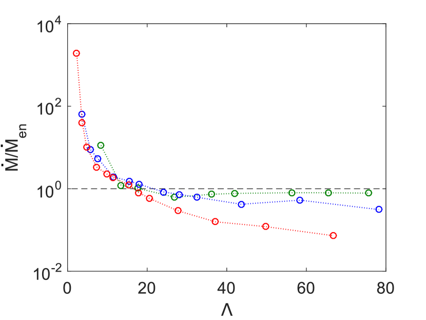
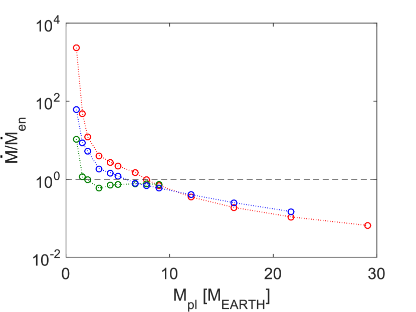
However, the plot in the top panel of Figure 4 might appear to be counterintuitive. This is because at large values the hotter planets, thus more likely to have a stable atmosphere, present mass-loss rates differing more from the energy-limited approximation than the cooler ones. This can be explained by the fact that for a given value of hotter planets have higher masses in comparison to cooler planets (see Equation (20)), therefore in this plot the hotter planets are more likely to have an hydrostatic atmosphere. This is clarified by the bottom panel of Figure 4, which shows that for the higher mass planets the difference between the mass-loss rates computed by the hydrodynamic model and with Equation (22) is independent of .
Equation (22) assumes that the entire stellar XUV energy input goes into driving the escape, but in reality part of this energy goes into running the chemical reactions, mainly ionisation of atomic hydrogen and dissociation of molecular hydrogen. Also, Erkaev et al. (2015) showed that the energy-limited formula neglects kinetic and thermal energy terms in the denominator, which can also be important for some star/planet parameters; i.e., even without including detailed chemistry or ionisation the results of Equation (22) should be higher than the hydrodynamic mass-loss rates for XUV-driven outflows. This explains why for most planets the energy-limited approximation overestimates the mass-loss rates. However, this is not the case when there is a significant component of thermal escape, in which case mass loss is driven partially by the stellar XUV flux and partially by the intrinsic planetary thermal energy. In this case, the mass-loss rates can significantly exceed those predicted by the energy-limited formula.
4.1 Grid interpolation
We developed a routine which interpolates the model results over the grid parameter space considering planetary mass, planetary radius, planetary equilibrium temperature, stellar mass, and stellar XUV flux. For any system with parameters covered by the grid, the routine extracts the density and outflow velocity, the mass-loss rate, the value of maximum temperature, the effective radius of XUV absorption, and the position of maximum dissociation and ionisation.
The routine performs the interpolation in the following consecutive steps.
-
1.
For planets with input parameters [, , , , ] the routine finds in the grid the two closest values of stellar mass and equilibrium temperature [, ], [, ].
-
2.
For each of the four combinations of [, ], with = 1,2, the routine finds the two closest values of the stellar XUV flux at the planetary orbital separation , with = 1,2 (i.e., eight values).
-
3.
For each set of [, , ] the atmospheric parameters depend therefore only on planetary radius and mass. Planets of the same mass have different atmospheric properties for different equilibrium temperatures, but we find similar atmospheric properties for planets with similar values. Therefore, we substitute planetary mass with . At this point, the routine interpolates the output parameters simultaneously over the pair [, ] for each of the eight sets of [, , ]. However, for planets beyond 0.1 AU, the simultaneous interpolation on and is not necessary, thus we reduced it to an interpolation on only.
-
4.
The routine interpolates the output parameters over .
-
5.
The same equilibrium temperature for different stellar masses occurs at rather different orbital separations (e.g., within the grid, a of K corresponds to distances ranging from 510-3 to 1.52 AU). Our analysis (see Section 5 and also Kubyshkina et al. 2018) indicates that between and , the latter has the larger influence on the results, thus for the interpolation we substitute with . Therefore, the routine interpolates the output parameters over for the pair of .
-
6.
The routine interpolates the output parameters over .
We developed this routine keeping in mind that the size of the grid will increase in the future, therefore the need of an interpolation routine capable of quickly handling the addition of grid points. This is why we avoided to use complicated, multi-dimensional interpolation functions that would require recomputing every time a new model is added to the grid.
Because the output parameters behave differently as a function of the input parameters, for almost each interpolation step and almost each output parameter, we employ a different function. For the mass-loss rates and the density at the Roche radius the routine interpolates over , , and according to
| (23) |
| (24) |
and
| (25) |
where X is either the mass-loss rate or the density at the Roche radius and the coefficients depend on the other system parameters. For planets in boil-off, Equations (23) and (24) are not accurate enough, therefore we use a piece-wise polynomial interpolation with input and output parameters in logarithmic scale. The interpolation of the mass-loss rates and the density at the Roche radius over the other input parameters (i.e., and ) is done on the basis of a linear function.
For the outflow velocity, we perform the interpolation on the [, ] pair using a third order polynomial function, which becomes linear for 20. For the interpolation of the outflow velocity over the other input parameters we use a linear function.
For the interpolation of the maximum temperature over each input parameter, we employ a linear function. The routine interpolates the position of the maximum dissociation and ionisation and of the value on the [, ] pair using a linear function for 20, while for smaller values we interpolate over using a function of the form , where the coefficients and depend on the other input parameters. For the interpolation of the maximum temperature, maximum dissociation and ionisation, and value over the other input parameters (i.e., , , and ) we employ a linear function.
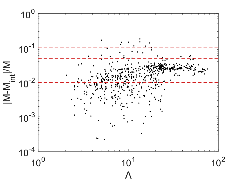
We performed two tests to validate the interpolation routine. We first compared the results obtained from the models with those derived using the interpolation for 500 systems randomly distributed across the grid. We found an agreement of better than 5% in 95% of the cases, while for the remaining systems the agreement was better than 20% (Figure 5).
The second test is dedicated to check the validity of substituting with for the interpolation. We used real planets for this test, namely Kepler-11 b, GJ 436 b, HAT-P 26 b, HD97658 b, GJ 3470 b, HAT-P 11 b, and 55 Cnc e, which lie within our grid boundaries, and compared the mass-loss rates obtained with direct modelling and interpolation. Figure 6 shows the results of this comparison, indicating that we obtain an excellent agreement for all of them. This validates our choice of interpolating on the orbital separation rather than on the planetary equilibrium temperature. We run the same test, but this time interpolating on the planetary equilibrium temperature, instead of orbital separation, obtaining significantly larger discrepancies.
5 Discussion
We discuss here in more detail how the results of the grid depend on the input parameters (Section 5.1) and briefly explore one of its possible future applications (Section 5.2). The reader not interested in the technicalities of the results can skip to Section 5.2, which is independent from what is described in Section 5.1.
5.1 Behaviour of the atmospheric parameters as a function of input parameters
The grid allows for the detailed description of how the atmospheric structure changes with respect to the input system parameters. The behaviour of the main output parameters can be separated into common patterns. We found a common behaviour between i) mass-loss rates and densities of the atmospheric species (Section 5.1.1); ii) effective radius of the stellar XUV absorption and position of the maximum dissociation and ionisation (Section 5.1.2); iii) outflow velocity and atmospheric temperature (Section 5.1.3).
5.1.1 Mass-loss rates and densities of the atmospheric species
One of the major parameters controlling the long-term evolution of a planetary atmosphere is the mass-loss rate , which strongly depends on the planetary gravity and orbital separation, thus the equilibrium temperature. Figure 6 shows the dependence of on . Within the parameters covered by our grid, the mass-loss rate varies by several orders of magnitude, with planetary gravity and Roche lobe radius being among the main parameters controlling it.
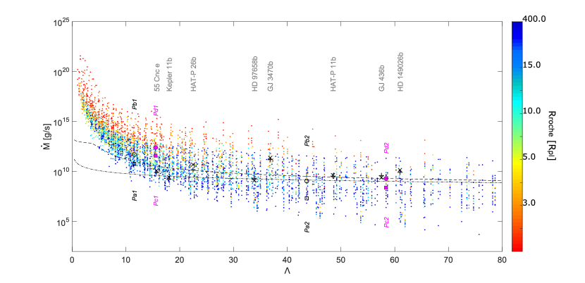
For the planets with values smaller than about 20, the escape rates reach extreme values of up to 1020 , due to a combination of low planetary gravities and high equilibrium temperatures (i.e., boil-off). The atmospheres of these planets are therefore characterised by strong thermal escape and inefficient XUV heating. The escape rates for the majority of these planets lie above the predictions of the energy-limited formula, and the energy budget of the atmosphere is dominated by adiabatic cooling. In first approximation, for a given stellar mass, , and stellar XUV flux, the dependence of the mass-loss rate on can be described by Equation (24). Such high escape rates would imply a rapid escape of the atmosphere (we provide a practical example of this in Section 5.2).
With increasing , the efficiency of XUV heating increases with XUV penetration depth (see Figure 2) and the mass-loss rates become strongly dependent on the stellar XUV flux. This further dependence of the mass-loss rates is partly responsible for the increased spread in mass-loss rates at large values. We also note that the spread increases with decreasing stellar mass, due to the decreasing orbital separation for the same temperature. The dependence of the mass-loss rates on the stellar XUV flux can be roughly described by a linear function, in agreement with the energy-limited formula.
Figure 6 shows also that the Roche radius plays an important role almost exclusively when it lies below about 15 (in Figure 6, the dark blue color corresponds to Roche radii ranging from 15 up to 400 ). It is important to remind that the Roche radius is tightly related with the orbital separation and the smallest Roche radii can be reached just for the shortest star-planet distances. As an example, within our grid, the smallest Roche radii (3 ) are reached only for planets lying less than 0.06 AU from the host star, while Roche radii of 15 are found for planets orbiting up to 0.3 AU from the host star. The mass-loss rates increase with decreasing Roche radii because a smaller Roche radius moves the sonic point closer to the planet, i.e., to regions of higher density, which leads to an increase in mass-loss rate. In addition, the Roche radius decreases with decreasing orbital separation (see Equation (1)), thus increasing and XUV irradiation.
To better illustrate how the escape rates change with input parameters, we set eight test planets (called Pa1, Pa2, Pb1, Pb2, Pc1, Pc2, Pd1, Pd2), whose parameters are listed in Table 4. The numbers “1” and “2” separate planets by mass, where the planets identified by the number “1” have the lower mass. The difference between the “a” & “b” and “c” & “d” planets is the stellar mass, which is higher for the former, while the difference between the “a” & “c” and “b” & “d” planets is the stellar XUV flux, which is higher for the latter. To have just the planetary mass controlling the value of , the eight planets have the same equilibrium temperature (700 K) and planetary radius (3 ). Figure 6 indicates the position of the eight planets in the vs plane.
| ID | |||||||||||
|---|---|---|---|---|---|---|---|---|---|---|---|
| [] | [K] | [] | [] | [] | [] | [] | [] | [K] | [] | ||
| Pa1 | 1.3 | 700 | 19.5 | 3 | 3.2 | 11.5 | 29.5 | 6.76 | 700 | 0.48 | |
| Pa2 | 1.3 | 700 | 19.5 | 3 | 12.1 | 43.6 | 45.9 | 1.90 | 1801 | 1.07 | |
| Pb1 | 1.3 | 700 | 1110.5 | 3 | 3.2 | 11.5 | 29.5 | 4.09 | 700 | 0.89 | |
| Pb2 | 1.3 | 700 | 1110.5 | 3 | 12.1 | 43.6 | 45.9 | 1.53 | 2318 | 2.25 | |
| Pc1 | 0.4 | 700 | 18.5 | 3 | 4.3 | 15.5 | 2.9 | 1.43 | 700 | 0.39 | |
| Pc2 | 0.4 | 700 | 18.5 | 3 | 16.2 | 58.4 | 4.6 | 1.15 | 3331 | 0.51 | |
| Pd1 | 0.4 | 700 | 16731 | 3 | 4.3 | 15.5 | 2.9 | 1.04 | 737 | 0.76 | |
| Pd2 | 0.4 | 700 | 16731 | 3 | 16.2 | 58.4 | 4.6 | 1.01 | 4370 | 1.37 |
As expected, an increase in the XUV stellar flux (i.e., PaPb or PcPd) or decrease in (i.e., Px2Px1, where x is any of a, b, c, or d) leads to an increase in the mass-loss rates. Figure 6 shows also that a decrease in stellar mass (i.e., PaPc or PbPd) leads as well to an increase in mass-loss rates. This is because, to maintain the same , planets orbiting around the lower mass star lie at a closer distance, thus have a smaller Roche radius and for the reasons described above have a higher mass-loss rate.
For the Pb planets, Figure 6 also compares the mass-loss rates with those predicted by the energy-limited formula assuming two different values for the effective radius and a heating efficiency of 15%, as for the hydrodynamic calculations. Since with decreasing the effective radius moves farther away from the planet, the distance between the two lines in Figure 6 increases with decreasing . The dashed line in Figure 6 presents a clear bend at 4, which is caused by the fact that at small values the effective radius reaches the Roche radius. Figure 6 indicates that at low values the energy-limited approximation significantly underestimates the escape rates (2–3 orders of magnitude; comparison to the black circles), while at large values the approximation overestimates the escape rates by about one order of magnitude (see also Figure 4).
The atmospheric densities (at the Roche radius) behave similarly to the mass-loss rates. The only small difference is found for planets with large values (densities decrease steeper). This is because the escape rates are calculated from the product of the atmospheric density and outflow velocity at the Roche radius, where the velocity increases with increasing Roche radius, which increases with increasing planetary mass.
The dependence of the escape rates and atmospheric densities on planetary mass is essentially the same as that on , though slightly less pronounced. The dependence of these parameters on is similar to what is displayed by the color code in Figure 6 and it can be described by using a log-linear approximation of the form , where X is either the mass-loss rate or the atmospheric density, and and are coefficients, which depend on the system parameters. This follows the high limit of the Parker wind problem.
5.1.2 Effective radius and position of the maximum dissociation and ionisation
We discuss here the behavior of three closely related parameters: the effective radius (Equation (21)) and the position of the maximum dissociation and ionisation. As we defined in Section 4, the position of the maximum dissociation and ionisation corresponds to the position of the maximum of and , respectively. Figure 7 shows the position of these three quantities as a function of . For most planets, they lie close to each other, except for planets with small values (i.e., 20), where the effective radius significantly exceeds the other two. At small values the effective radius can be up to ten times larger than the position of the maximum dissociation/ionisation, which stays close to one another for the whole interval of parameters. For values above 50, the difference between the position of maximum dissociation/ionisation and the effective radii lies roughly within 30%. We also found that for these planets the difference between the three values decreases slightly with increasing stellar XUV flux and planetary mass, where the latter dependence is caused by the gradual compression of the atmosphere with increasing planetary mass.
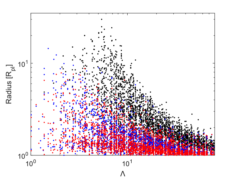
The possible range of values found in the grid for the effective radius and the position of the maximum dissociation and ionisation increases significantly with decreasing and it reaches the maximum close to = 5. Here the effective radius reaches the Roche radius, which decreases with decreasing . The position of maximum dissociation/ionisation reaches this artificial border at smaller values, i.e., 2.
We found also a clear dependence of the three quantities on orbital separation. To highlight this, Figure 8 shows the effective radius as a function of the Roche radius and of the orbital separation. Again, for each given Roche radius, the effective radius presents an upper limit, which is clearly given by itself. The spread in effective radii also increases with increasing and . This can be understood as follows. At short orbital separations, is generally small and therefore there is only a small range of possible effective radii. At large orbital separations, instead, depending on the planetary and stellar masses, there is a much wider range of possible Roche radii within which the position of maximum dissociation can lie. However, Figure 8 shows that in our grid there are very few planets with large Roche and effective radii, namely those with a rather low-density and orbiting far from the host stars. For these planets, is large and the stellar XUV flux is too weak for the effective radius to be close to .
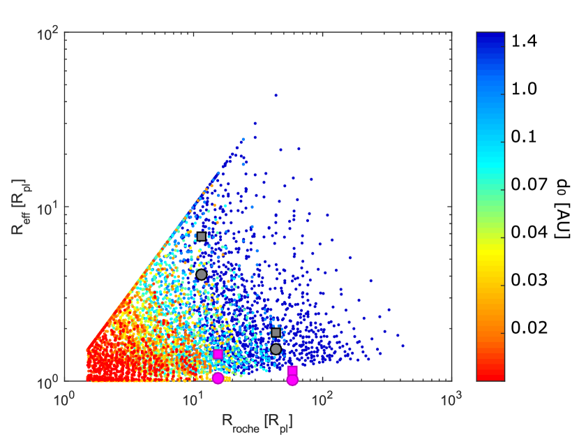
Finally, there are a few remarks that need to be made regarding these parameters. Unlike the definition of the effective radius (given by Equation (21)), the definitions of the position of maximum dissociation and ionisation are not univocal. In addition, in some cases, the dissociation and ionisation profiles are very smooth, which makes the position of maximum dissociation and ionisation somewhat dependent on their definitions. It is artificial to consider that the effective radius and/or the position of the maximum ionisation and dissociation are located at the Roche lobe if their position moves beyond it. It is therefore important to keep in mind that for some particular planets these values are indicative, rather than sharp results, and that comparisons with the literature and/or with future studies shall consider these issues.
5.1.3 Outflow velocity at the Roche radius and maximum atmospheric temperature
We define the outflow velocity as the velocity of the atmospheric particles crossing the Roche lobe. Figure 9 shows the velocity at the Roche radius as a function of and orbital semi-major axis. For planets with values 10, the velocity of the escaping material grows linearly with increasing . This is caused by the gradual increase of the Roche radius with , which allows for longer acceleration distances and for a smaller planetary gravitational pull at the Roche radius. This lies partly at the origin of the connection between the velocity at the Roche radius and orbital semi-major axis.
For planets with very small values, the velocity behaves exactly in the opposite way, it increases with decreasing as a result of the low gravity and small Roche radius. We found that the planets for which is larger than 2 have a Roche radius located closer than 5 , while for more extreme planets with greater than 4 , the Roche radius is always smaller than 1.5 .
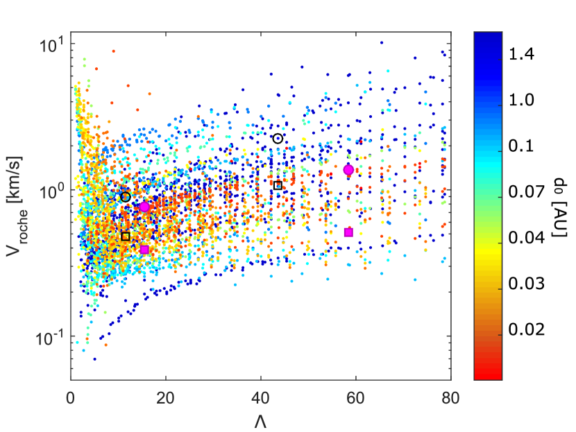
The dependence of the outflow velocity on the XUV flux is similar to that of the mass-loss rates. To illustrate this, we added the position of the eight test planets to Figure 9. The influence of the equilibrium temperature on the velocity at the Roche radius is however unclear, possibly because variations in the equilibrium temperature imply simultaneous changes in the atmospheric structure and in the orbital separation, thus in the Roche radius. In Kubyshkina et al. (2018), we showed that, keeping planetary mass and radius fixed, the effects of variations on the velocity are negligible for planets with greater than 20, while for planets with lower the velocity may significantly decrease with increasing temperature.
We found that the maximum value of the atmospheric temperature behaves similarly to the outflow velocity, except for planets with small values (15–20). For these planets, the atmospheric temperature profile is characterised by strong adiabatic cooling, which implies that the maximum temperature is equal to the equilibrium temperature. For planets with larger values, the maximum atmospheric temperature increases almost linearly with , similarly to the velocity, but it further presents a more pronounced dependence on the stellar XUV flux.
5.2 Atmospheric evolution of the high-density exoplanets CoRoT-7 b and HD219134 b,c
We present here a direct application of the grid, namely a simple scheme allowing to infer the evolution of a planetary atmosphere subject to mass-loss, with the mass-loss rates extracted from the grid. Thanks to the dense grid and possibility to interpolate across it, one can quickly derive high-resolution evolutionary tracks of planets with parameters contained in the grid. The advantage is that the tracks are obtained making use of mass-loss rates computed with an hydrodynamic code, rather than more approximate methods, such as the energy-limited formula. As an example, we study the past evolution of the possible primary atmospheres of the close-in high-density planets CoRoT-7 b (Léger et al. 2009; Valencia et al. 2010; Leitzinger et al. 2011; Mura et al. 2011; Barros et al. 2014) and HD219134 b,c (Motalebi et al. 2015; Vogt et al. 2015; Gillon et al. 2017).
5.2.1 Planetary evolution modelling scheme
We first assume that the orbital separation and stellar mass do not change with time. It follows that the mass-loss rates at every moment in time depend only on the planetary radius and the amount of bolometric and XUV stellar irradiation.
To infer planetary atmospheric mass fractions (), we employ the model described by Johnstone et al. (2015), which relates with planetary mass and radius. However, the approximate relation between these three quantities given by Johnstone et al. (2015) was obtained considering atmospheres having a density of 51012 cm-3 and a temperature of 250 K at the base of the simulation, which significantly differ from the conditions of our planets. Therefore, we used the code employed by Johnstone et al. (2015) to directly compute a grid of values ((hereafter called -grid) for planets with mass and radius in the range of interest of this work and interpolate among the grid points. For each planet considered in the -grid, the core radius was derived assuming an Earth-like density.
One of the key parameters to set to simulate the atmospheric evolution is the initial planetary radius. Various accretion models provide an estimate of the initial planetary radius, thus atmospheric mass accreted by the planet while embedded in the protoplanetary nebula (e.g., Stökl et al. 2016), but the results are rather model dependent and small variations may affect the tracks. We approach this problem in a more empirical way: we calculate tracks assuming three different initial radii and see a posteriori which is the impact of the assumption of the initial radius on the evolutionary tracks. As initial radii for each planet, we assume the values obtained by setting equal to 3, 5, and 10.
For late-type stars, the stellar XUV flux depends on the stellar mass and rotation period, where the latter is time-dependent. In this work, we assume that the rotation period varies with time as (Mamajek & Hillenbrand 2008)
| (26) |
where is the rotation period (in days), is the stellar age (in Myr), and is the reddening-free stellar color. Equation (26) represents the average approximation based on a large set of late-type dwarfs, but in reality the rotation tracks of stars are non-unique, which leads to different evolutionary tracks of the XUV radiation (Johnstone et al. 2015b; Tu et al. 2015). In the most general case, this results in a variety of planetary atmosphere evolution tracks, but for the present analysis that is limited to small, close-in planets we restrict ourselves to the approximation given by Equation 26.
We set the relevant stellar parameters as follows. The stellar X-ray flux can then be inferred from the rotation period as (Wright et al. 2011)
| (27) |
where is the X-ray stellar luminosity, is the bolometric luminosity, = 8.6810-6 and = 2.18 are empirical constants (Pizzolato et al. 2003; Wright et al. 2011), and = 0.13 is the saturation threshold corresponding to the Rossby number . This last quantity is the ratio between the stellar rotation period and the convective turnover time (; Wright et al. 2011)
| (28) |
The EUV stellar luminosity is then derived from the X-ray luminosity using Equation (19). To account for how the bolometric luminosity and equilibrium temperature change with time, we employ the MESA Isochrones and Stellar Tracks (MIST; Paxton et al. 2018).
We begin the evolution at the age of 5 Myr, which is approximately the typical lifetime of protoplanetary disks (Mamajek 2009). However, since we are in general interested in Gyrs-old planets, the exact initial time for the evolution has no significant effect on the results. Having set the initial planetary radius, , and XUV stellar flux at the planetary orbital separation, we extract the mass-loss rate from our grid, which we then use to derive how much mass is lost during the first time step. At this point, we derive the new planetary atmospheric mass that we convert into a planetary radius by interpolating over the -grid, and begin the cycle again, updating at each time step the stellar XUV flux. We finally obtain atmospheric evolutionary tracks by choosing small-enough time steps, which in our case adapt to the mass-loss rates by ensuring that the maximum mass loss within one time step is smaller than 1% of the planetary mass, and by repeating this procedure up to the desired age (e.g., age of the given system) or till the planetary radius has reached the core radius. We ignore gravitational contraction and radioactive decay that contribute to increase the equilibrium temperature during the first phases of evolution.
5.2.2 Results for CoRoT-7 b
CoRoT-7 b has a mass of 5.74 and a radius of 1.585 , which indicates a rocky composition and a lack of a hydrogen-dominated envelope (Léger et al. 2009; Mura et al. 2011; Barros et al. 2014). The planet orbits an active early K-type star ( = 0.93 , = 0.87 , = 5275 K) at a distance of 0.0172 AU, which corresponds to a period of 0.853 days. The planet has an equilibrium temperature of 1756 K and the age of the system has been estimated to be 1.50.3 Gyr.
Figure 10 shows the evolution of the planetary radius as a function of time obtained for each of the three tested initial conditions corresponding to planetary radii of 8.25 (), 4.95 (), and 2.47 (). The two tracks starting with the largest planetary radius converge quickly to the same point, implying that the result is independent of the initial condition. This is because the first part of the evolution is dominated by boil-off. The track starting with the smaller planetary radius instead does not present clear signs of a boil-off phase, but still leads to a rapid complete escape of the atmosphere. The tracks indicate that the planet is supposed to have completely lost its hydrogen-dominated envelope within an extremely short time of about 0.1 Myr.
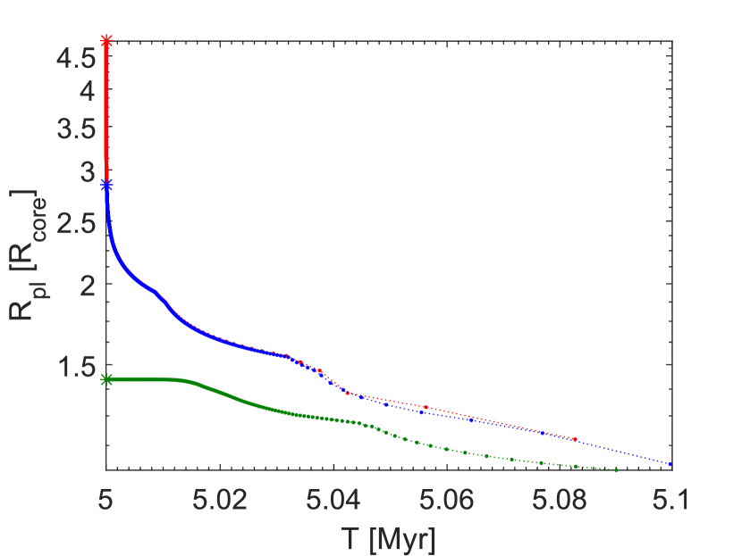
The most significant changes in the size of the atmosphere occur during the first Myr, when the atmosphere lies in the boil-off regime, which is consistent with what was found by Owen & Wu (2016). Once the radius has reached about 2 , the escape is driven by the stellar XUV flux, which for CoRoT-7 b is very intense since the system is still rather young and the planet has a very short orbital period. The complete escape of the atmosphere is so fast that the initial stellar rotation rate (see, e.g., Tu et al. 2015) does not play a significant role. We therefore estimate that CoRoT-7 b has lost its primary atmosphere, assuming it had accreted one to begin with, within a maximum time of about 0.1 Myr.
Atmospheric escape for CoRoT-7 b has been previously studied by Jackson et al. (2010) and Leitzinger et al. (2011). Both inferred the planet’s mass-loss rate over time using the energy-limited approximation, accounting for the Roche lobe effect (Erkaev et al. 2007), which greatly underestimates the mass-loss rates at the beginning of the planet’s evolution.
Jackson et al. (2010) considered the effects of the possible planetary migration through orbital tidal decay, a wide range of initial radii (up to a gas giant), an effective radius of 3 , various heating efficiencies up to 100%, and applied the scaling laws for the stellar XUV flux of Ribas et al. (2005). They arrived at the conclusion that CoRoT-7 b could have started its evolution as a gas giant, with a mass of up to 200 . In case, instead, CoRoT-7 b has always been a rocky planet, they suggested that it could have lost up to half of its mass through surface melting, outgassing, and subsequent escape of the secondary atmosphere.
Leitzinger et al. (2011) did not account for planetary migration, but employed more realistic heating efficiencies of 10-25% and stellar irradiation levels consistent with those adopted in our work. Their calculations led them to exclude that CoRoT-7 b had started its evolution as a gas giant planet, with a mass similar or larger than that of Saturn, otherwise the planet would still host a significant hydrogen-dominated envelope, which is excluded by the Earth-like bulk density.
At the very beginning of the evolution, when the planetary atmosphere is supposed to be in boil-off, the mass-loss rates derived from the grid are larger than those considered by Jackson et al. (2010) and Leitzinger et al. (2011) by a factor of 10–106, depending on the initial planetary radius. This large difference is caused by the fact that the energy-limited approximation is not capable of describing atmospheric escape in the boil-off phase. In the blow-off phase, instead, the mass-loss rates derived from the grid are about a factor of two smaller than those of Leitzinger et al. (2011) and a factor of a few smaller than those of Jackson et al. (2010).
Following the works of Jackson et al. (2010) and Leitzinger et al. (2011), we further tested the possible evolution of CoRoT-7 b by increasing even more the initial planetary mass (and radius) obtaining that the planet needed to have a mass smaller than that of Uranus (about 14.5 ) to loose the primary atmosphere within the age of the system. An initial CoRoT-7 b with a mass equal to that of Neptune (about 17 ) would now still hold a hydrogen-dominated envelope with = 0.2. We did not explore an even heavier starting point because of the upper mass limit of 39 in our grid.
5.2.3 Results for HD219134 b,c
HD219134 b,c are two close-in, transiting super-Earths orbiting a K3 main-sequence star with a radius of 0.778 , a mass of 0.81 , and an effective temperature of 4699 K. The estimated age of the system is 112 Gyr. The two planets have measured masses of 5.74 and 4.74 , and radii of 1.602 and 1.511 , respectively. Therefore, both planets present Earth-like densities. They orbit the host star at distances of 0.039 and 0.065 AU, respectively.
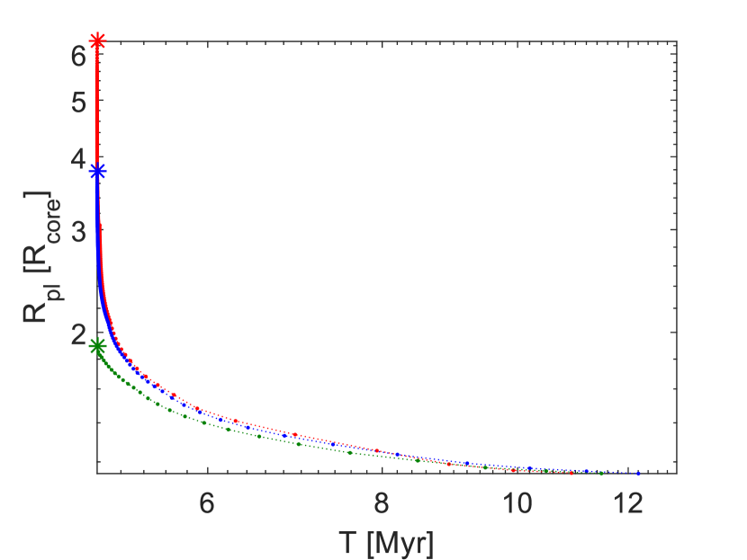
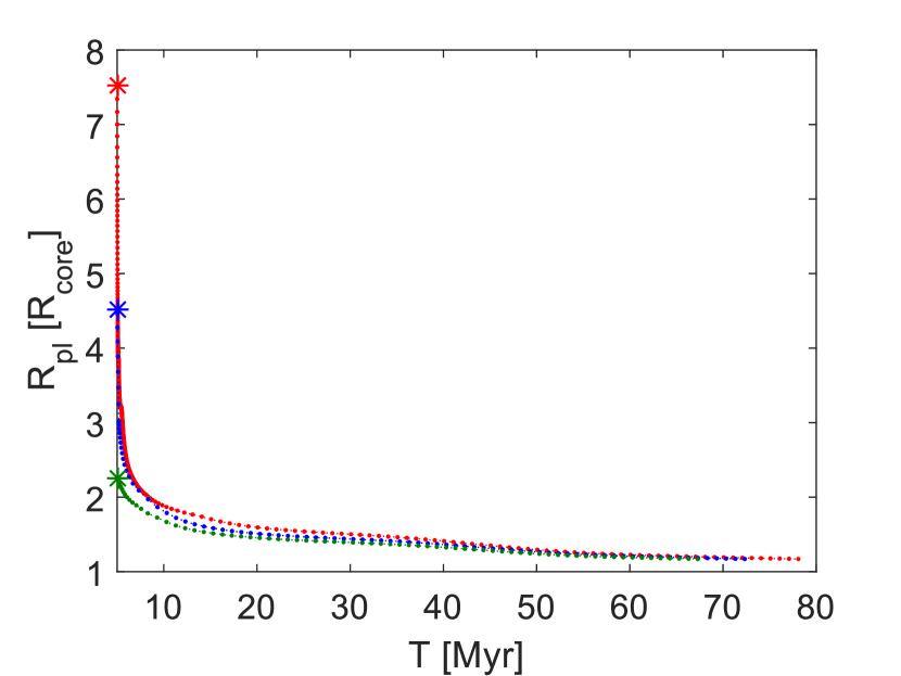
The evolutionary tracks, shown in Figure 11, indicate that the primary, hydrogen-dominated atmosphere escaped completely within about 12 and 80 Myr for HD219134 b,c, respectively. The difference in time between the two planets for a complete atmospheric escape is due to their different distance from the star, thus different equilibrium temperature and stellar XUV irradiation. These times are significantly shorter than the estimated age of the system, thus allowing us to conclude that both planets have most likely completely lost their primary, hydrogen-dominated atmosphere through escape. This is in agreement with Dorn & Heng (2018), who arrived at the same conclusion by employing a Bayesian inference method based on the stellar properties and the energy-limited approximation. However, these are extreme cases, and an approach based on the energy-limited formulation would most likely lead to the wrong results for younger and/or lower density planets.
6 Conclusion
We upgraded and employed an existing planetary upper atmosphere hydrodynamic code to compute a large grid of models for super-Earths and mini-Neptunes orbiting late-type stars. The main upgrade consists in the implementation of a scheme that automatically sets the initial parameters and profiles for each run, thus in practice allowing one to automate computations. The planets covered by the grid have masses ranging from 1 to 39 and orbit early M- to late F-type stars in a wide range of orbital distances, corresponding to equilibrium temperatures between 300 and 2000 K. For each considered stellar mass, we have also considered three different values of the XUV flux. The wide parameter space covered by the grid allowed us to model a broad variety of planetary atmospheres, ranging from being in boil-off, to blow-off, and to very stable atmospheres.
For each planet in the grid, we computed the atmospheric temperature, number density, bulk velocity, X-ray and EUV volume heating rates, and abundance of the considered species as a function of distance from the planetary center. From these quantities, we estimated the positions of maximum dissociation and ionisation, the mass-loss rate, and the effective radius of the XUV absorption.
We compared the results of our grid, in particular the mass-loss rates, with those previously published for planets inside and outside the grid boundaries, finding excellent agreement. We also developed a tool to interpolate among the model results to infer the atmospheric properties of any planet covered by the grid. We took advantage of the large grid to explore in detail how the atmospheric characteristics vary with system parameters, finding for example that the mass-loss rate can be analytically described as a log-linear function of and a linear function of the stellar XUV flux.
Our grid and the interpolation routine allow one to extract in a fraction of a second information that would otherwise require days/weeks to obtain. This enables one to employ the results of proper hydrodynamic computations of the mass-loss rates in planetary atmospheric evolution calculations. This avoids the need to use approximations, such as the energy-limited formula, that have been shown (by various authors and further in this work) to significantly underestimate or overestimate in some cases the mass-loss rates.
We have therefore applied our grid and interpolation routine to study the evolution of the close-in, high-density planets CoRoT-7 b and HD219134 b,c. For CoRoT-7 b, we found that the primary hydrogen-dominated atmosphere, assuming the planet has ever accreted one, was lost mostly through boil-off within about 0.1 Myr. We also concluded that the planet originally could have been as massive as Uranus, because the envelope of a heavier planet would have been too massive to completely escape within the age of the system. We arrived at a similar conclusion also for HD219134 b,c, where for these two planets we found that the hydrogen-dominated atmosphere escaped completely within about 12 and 80 Myr, respectively. It is therefore likely that other similar planets, such as Kepler-10b and 55 Cnc e, followed an analogous evolutionary path, which have left them with a secondary atmosphere formed by either outgassing from the magma ocean or sputtering of the stellar wind on the bare planetary surface, similar to what happens for Mercury (Mura et al. 2011; Guenther et al. 2011; Pfleger et al. 2015; Vidotto et al. 2018).
The simple evolutionary tracks we computed for CoRoT-7 b and HD219134 b,c provide just an example of what can be achieved using the grid and interpolation routine. There is, however, a large number of applications in which these tools can be used and we will explore a few of them (e.g., analytic formulation of the mass-loss rates as a function of system parameters) in future works currently in preparation. We are still working on increasing the size of the grid, extending it towards more massive planets and towards less massive stars. The grid and interpolation routine can be downloaded here http://geco.oeaw.ac.at/links_TAPAS4CHEOPS.html. We are, however, planning for the near future to set up a web interface allowing users to more easily query the grid and run the interpolation routine.
Acknowledgements.
We acknowledge the Austrian Forschungsförderungsgesellschaft FFG project “TAPAS4CHEOPS” P853993, the Austrian Science Fund (FWF) NFN project S11607-N16, the FWF project P27256-N27 and the FWF project P30949-N36. NVE acknowledges support by the RFBR grant No. 18-05-00195-a and 16-52-14006 ANF_a. We thank the anonymous referee for the positive approach and the useful comments that led to a significant improvement of the manuscript.References
- Barros et al. (2014) Barros, S. C. C., Almenara, J. M., Deleuil, M., et al. 2014, A&A, 569, A74
- Barclay et al. (2018) Barclay, T., Pepper, J., & Quintana, E. V. 2018, AJ, submitted (arXiv:1804.05050)
- Batygin & Stevenson (2013) Batygin, K., & Stevenson, D. J. 2013, ApJ, 769, L9
- Black (1981) Black, J. H. 1981, MNRAS, 197, 553,
- Bonfils et al. (2013) Bonfils, X., Delfosse, X., Udry, S., et al. 2013, A&A, 549, A109
- Bourrier & Lecavelier des Etangs (2013) Bourrier, V., & Lecavelier des Etangs, A. 2013, A&A, 557, A124
- Bourrier et al. (2016) Bourrier, V., Lecavelier des Etangs, A., Ehrenreich, D., Tanaka, Y. A., & Vidotto, A. A. 2016, A&A, 591, A121
- Broeg et al. (2013) Broeg, C., Fortier, A., Ehrenreich, D., et al. 2013, European Physical Journal Web of Conferences, 47, 03005
- Cecchi-Pestellini et al. (2009) Cecchi-Pestellini, C., Ciaravella, A., Micela, G., & Penz, T. 2009, A&A, 496, 863
- Chamberlain (1963) Chamberlain, J. W. 1963, Planet. Space Sci., 11, 901
- Chen & Rogers (2016) Chen, H., & Rogers, L. A. 2016, ApJ, 831, 180
- Cubillos et al. (2017a) Cubillos, P., Erkaev, N. V., Juvan, I., et al. 2017a, MNRAS, 466, 1868
- Cubillos et al. (2017b) Cubillos, P. E., Fossati, L., Erkaev, N. V., et al. 2017b, ApJ, 849, 145
- Deming et al. (2009) Deming, D., Seager, S., Winn, J., et al. 2009, PASP, 121, 952
- Dorn & Heng (2018) Dorn, C., & Heng, K. 2018, ApJ, 853, 64
- Ehrenreich et al. (2008) Ehrenreich, D., Lecavelier Des Etangs, A., Hébrard, G., et al. 2008, A&A, 483, 933
- Ehrenreich and Désert (2011) Ehrenreich and Désert A&A, 2011
- Ehrenreich et al. (2015) Ehrenreich, D., Bourrier, V., Wheatley, P. J., et al. 2015, Nature, 522, 459
- Erkaev et al. (2007) Erkaev, N. V., Kulikov, Y. N., Lammer, H., et al. 2007, A&A, 472, 329
- Erkaev et al. (2013) Erkaev, N. V., Lammer, H., Odert, P., et al. 2013, Astrobiology, 13, 1011
- Erkaev et al. (2014) Erkaev, N. V., Lammer, H., Elkins-Tanton, L. T., et al. 2014, Planet. Space Sci., 98, 106
- Erkaev et al. (2015) Erkaev, N. V., Lammer, H., Odert, P., Kulikov, Y. N., & Kislyakova, K. G. 2015, MNRAS, 448, 1916
- Erkaev et al. (2016) Erkaev, N. V., Lammer, H., Odert, P., et al. 2016, MNRAS, 460, 1300
- Erkaev et al. (2017) Erkaev, N. V., Odert, P., Lammer, H., et al. 2017, MNRAS, 470, 4330
- Fleming et al. (2018) Fleming, B. T., France, K., Nell, N., et al. 2018, Journal of Astronomical Telescopes, Instruments, and Systems, 4, 014004
- Fossati et al. (2015) Fossati, L., France, K., Koskinen, T., et al. 2015, ApJ, 815, 118
- Fossati et al. (2017) Fossati, L., Erkaev, N. V., Lammer, H., et al. 2017, A&A, 598, A90
- Fossati et al. (2018) Fossati, L., Koskinen, T., France, K., et al. 2018, AJ, 155, 113
- Fulton et al. (2017) Fulton, B. J., Petigura, E. A., Howard, A. W., et al. 2017, AJ, 154, 109
- Fulton & Petigura (2018) Fulton, B. J., & Petigura, E. A. 2018, AJ, submitted (arXiv:1805.01453)
- Gardner et al. (2006) Gardner, J. P., Mather, J. C., Clampin, M., et al. 2006, Space Sci. Rev., 123, 485
- Gillon et al. (2017) Gillon, M., Demory, B.-O., Van Grootel, V., et al. 2017, Nature Astronomy, 1, 0056
- Ginzburg et al. (2016) Ginzburg, S., Schlichting, H. E., & Sari, R. 2016, ApJ, 825, 29
- Ginzburg et al. (2018) Ginzburg, S., Schlichting, H. E., & Sari, R. 2018, MNRAS, 476, 759
- Guenther et al. (2011) Guenther, E. W., Cabrera, J., Erikson, A., et al. 2011, A&A, 525, A24
- Guo & Ben-Jaffel (2016) Guo, J. H., & Ben-Jaffel, L. 2016, ApJ, 818, 107
- Howe et al. (2014) Howe, A. R., Burrows, A., & Verne, W. 2014, ApJ, 787, 173
- Jackson et al. (2010) Jackson, B., Miller, N., Barnes, R., et al. 2010, MNRAS, 407, 910
- Jackson et al. (2012) Jackson, A. P., Davis, T. A., & Wheatley, P. J. 2012, MNRAS, 422, 2024
- Jeans (1925) Jeans, J. 1925, The Dynamical Theory of Gases. By Sir James Jeans. Cambridge University Press, 1925. ISBN: 978-1-1080-0564-7
- Jin et al. (2014) Jin, S., Mordasini, C., Parmentier, V., et al. 2014, ApJ, 795, 65
- Jin & Mordasini (2017) Jin, S., & Mordasini, C. 2018, ApJ, 853, 163
- Johnstone et al. (2015) Johnstone, C. P., Güdel, M., Stökl, A., et al. 2015, ApJ, 815, L12
- Johnstone et al. (2015b) Johnstone, C. P., Güdel, M., Brott, I., & Lüftinger, T. 2015, A&A, 577, A28
- Kislyakova et al. (2014) Kislyakova, K. G., Johnstone, C. P., Odert, P., et al. 2014, A&A, 562, A116
- Koskinen et al. (2010) Koskinen, T. T., Yelle, R. V., Lavvas, P., & Lewis, N. K. 2010, ApJ, 723, 116
- Koskinen et al. (2013) Koskinen, T. T., Harris, M. J., Yelle, R. V., & Lavvas, P. 2013, Icarus, 226, 1678
- Kubyshkina et al. (2018) Kubyshkina, D., Lendl, M., Fossati, L., et al. 2018, A&A, 612, A25
- Lammer et al. (2003) Lammer, H., Selsis, F., Ribas, I., et al. 2003, ApJ, 598, L121
- Lammer et al. (2009) Lammer, H., Odert, P., Leitzinger, M., et al. 2009, A&A, 506, 399
- Lammer et al. (2013) Lammer, H., Erkaev, N. V., Odert, P., et al. 2013, MNRAS, 430, 1247
- Lammer et al. (2016) Lammer, H., Erkaev, N. V., Fossati, L., et al. 2016, MNRAS, 461, L62
- Lecavelier des Etangs et al. (2004) Lecavelier des Etangs et al. 418, L1, A&A2004
- Leitzinger et al. (2011) Leitzinger, M., Odert, P., Kulikov, Y. N., et al. 2011, Planet. Space Sci., 59, 1472
- Léger et al. (2009) Léger, A., Rouan, D., Schneider, J., et al. 2009, A&A, 506, 287
- Lopez & Fortney (2013) Lopez, E. D., & Fortney, J. J. 2013, ApJ, 776, 2
- Lopez & Fortney (2014) Lopez, E. D., & Fortney, J. J. 2014, ApJ, 792, 1
- Lopez (2017) Lopez, E. D. 2017, MNRAS, 472, 245
- Lundkvist et al. (2016) Lundkvist, M. S., Kjeldsen, H., Albrecht, S., et al. 2016, Nature Communications, 7, 11201
- Mamajek & Hillenbrand (2008) Mamajek, E. E., & Hillenbrand, L. A. 2008, ApJ, 687, 1264-1293
- Mamajek (2009) Mamajek, E. E. 2009, American Institute of Physics Conference Series, 1158, 3
- Masuda (2014) Masuda, K. 2014, ApJ, 783, 53
- Menager et al. (2013) Menager, H., Barthélemy, M., Koskinen, T., et al. 2013, Icarus, 226, 1709
- Miller et al. (2013) Miller, S., Stallard, T., Tennyson, J., & Melin, H. 2013, Journal of Physical Chemistry A, 117, 9770
- Motalebi et al. (2015) Motalebi, F., Udry, S., Gillon, M., et al. 2015, A&A, 584, A72
- Mullally et al. (2015) Mullally, F., Coughlin, J. L., Thompson, S. E., et al. 2015, ApJS, 217, 31
- Mura et al. (2011) Mura, A., Wurz, P., Schneider, J., et al. 2011, Icarus, 211, 1
- Murray-Clay et al. (2009) Murray-Clay, R. A., Chiang, E. I., & Murray, N. 2009, ApJ, 693, 23
- Öpik (1963) Öpik, E. J. 1963, Geophysical Journal, 7, 490
- Owen & Jackson (2012) Owen, J. E., & Jackson, A. P. 2012, MNRAS, 425, 2931
- Owen & Mohanty (2016) Owen, J. E., & Mohanty, S. 2016, MNRAS, 459, 4088
- Owen & Wu (2016) Owen, J. E., & Wu, Y. 2016, ApJ, 817, 107
- Owen & Wu (2017) Owen, J. E., & Wu, Y. 2017, ApJ, 847, 29
- Paxton et al. (2018) Paxton, B., Schwab, J., Bauer, E. B., et al. 2018, ApJS, 234, 34
- Pfleger et al. (2015) Pfleger, M., Lichtenegger, H. I. M., Wurz, P., et al. 2015, Planet. Space Sci., 115, 90
- Pizzolato et al. (2003) Pizzolato, N., Maggio, A., Micela, G., Sciortino, S., & Ventura, P. 2003, A&A, 397, 147
- Quirrenbach et al. (2010) Quirrenbach, A., Amado, P. J., Mandel, H., et al. 2010, Proc. SPIE, 7735, 773513
- Rauer et al. (2014) Rauer, H., Catala, C., Aerts, C., et al. 2014, Experimental Astronomy, 38, 249
- Reiners et al. (2014) Reiners, A., Schüssler, M., & Passegger, V. M. 2014, ApJ, 794, 144
- Ribas et al. (2005) Ribas, I., Guinan, E. F., Güdel, M., & Audard, M. 2005, ApJ, 622, 680
- Ricker et al. (2015) Ricker, G. R., Winn, J. N., Vanderspek, R., et al. 2015, Journal of Astronomical Telescopes, Instruments, and Systems, 1, 014003
- Rodríguez et al. (2016) Rodríguez, A., Callegari, N., & Correia, A. C. M. 2016, MNRAS, 463, 3249
- Salz et al. (2016) Salz, M., Schneider, P. C., Czesla, S., & Schmitt, J. H. M. M. 2016, A&A, 585, L2
- Sanz-Forcada et al. (2011) Sanz-Forcada, J., Micela, G., Ribas, I., et al. 2011, A&A, 532, A6
- Shematovich et al. (2014) Shematovich, V. I., Ionov, D. E., & Lammer, H. 2014, A&A, 571, A94
- Spitzer (1978) Spitzer, L. 1978, Physical processes in the interstellar medium, by Lyman Spitzer. New York Wiley-Interscience, 1978, 333
- Storey & Hummer (1995) Storey, P. J., & Hummer, D. G. 1995, MNRAS, 272(1), 41-48
- Stökl et al. (2015) Stökl, A., Dorfi, E., & Lammer, H. 2015, A&A, 576, A87
- Stökl et al. (2016) Stökl, A., Dorfi, E. A., Johnstone, C. P., & Lammer, H. 2016, ApJ, 825, 86
- Tinetti et al. (2017) Tinetti, G., Drossart, P., Eccleston, P., et al. 2017, European Planetary Science Congress, 11, EPSC2017-713
- Tu et al. (2015) Tu, L., Johnstone, C. P., Güdel, M., & Lammer, H. 2015, A&A, 577, L3
- Valencia et al. (2010) Valencia, D., Ikoma, M., Guillot, T., & Nettelmann, N. 2010, A&A, 516, A20
- Van Eylen et al. (2017) Van Eylen, V., Agentoft, C., Lundkvist, M. S., et al. 2018, MNRAS, 479, 4786
- Vidotto et al. (2018) Vidotto, A. A., Lichtenegger, H., Fossati, L., et al. 2018, MNRAS, in press (arXiv:1808.00404)
- Vogt et al. (2015) Vogt, S. S., Burt, J., Meschiari, S., et al. 2015, ApJ, 814, 12
- Watson et al. (1981) Watson, A. J., Donahue, T. M., & Walker, J. C. G. 1981, Icarus, 48, 150
- Weiss & Marcy (2014) Weiss, L. M., & Marcy, G. W. 2014, ApJ, 783, L6
- Wolfgang et al. (2016) Wolfgang, A., Rogers, L. A., & Ford, E. B. 2016, ApJ, 825, 19
- Wright et al. (2011) Wright, N. J., Drake, J. J., Mamajek, E. E., & Henry, G. W. 2011, ApJ, 743, 48
- Yelle (2004) Yelle, R. V. 2004, Icarus, 170, 167
- Yi et al. (2001) Yi, S., Demarque, P., Kim, Y.-C., et al. 2001, ApJS, 136, 417
Appendix A List of reactions and cross-sections employed in the model
The reactions and cross-sections employed in the model are presented in Table 5.
Appendix B Normalisations employed for the computation of each model
Here we give the normalisations used for the computation of the models.
In the equations above, the subscript “0” denotes the values at the lower boundary, e.g., and are respectively the pressure and sound speed at the lower boundary.
Appendix C Planetary atmospheric mass-loss rates as a function of system parameters
We present here plots analogous to those in Figure 3, but for different stellar masses (Figures 12 to 15).
au au au
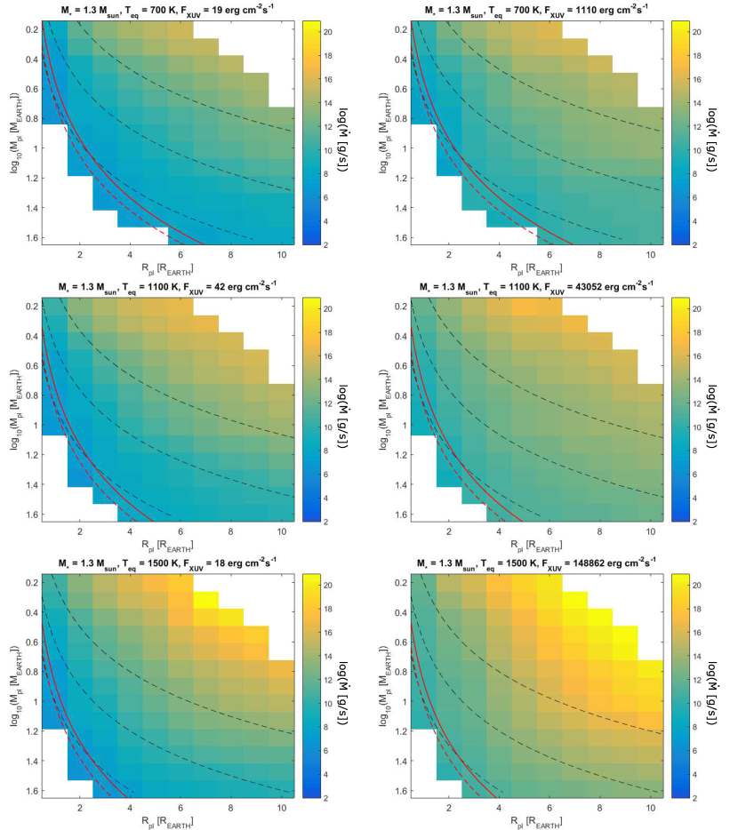
au au au
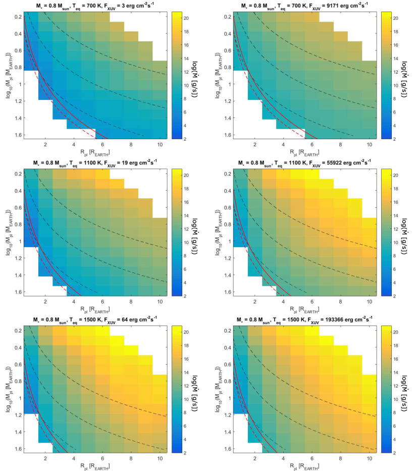
au au au
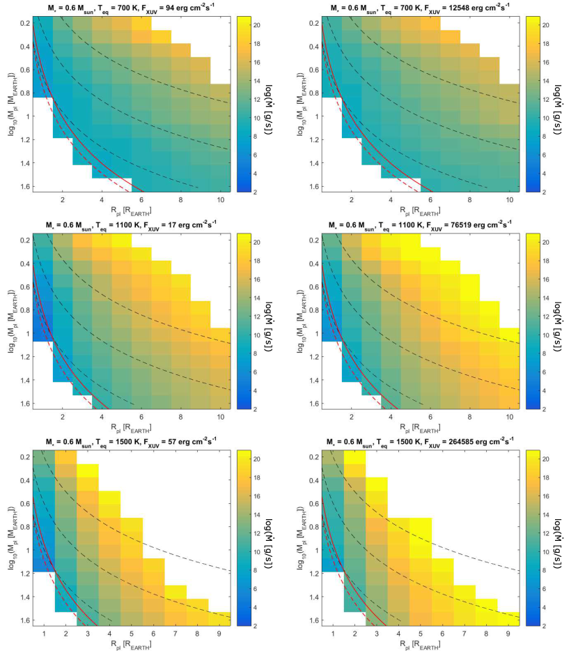
au au au
