Interface sensitivity on spin transport through a three-terminal graphene nanoribbon

Abstract

Spin dependent transport in a three-terminal graphene nanoribbon (GNR) is investigated in presence of Rashba spin-orbit interaction. Such a three-terminal structure is shown to be highly effective in filtering electron spins from an unpolarized source simultaneously into two output leads and thus can be used as an efficient spin filter device compared to a two-terminal one. The study of sensitivity of the spin-polarized transmission on the location of the outgoing leads results in interesting consequences and is explored in details. There exist certain symmetry relations between the two outgoing leads with regard to spin-polarized transport, especially when they are connected to the system in a particular manner. We believe that the prototype presented here can be realized experimentally and hence the results can also be verified.

I Introduction

In the last two decades, spintronics has emerged as one of the most active research fields in condensed matter physics, material science, and nanotechnology. The main goal of spintronics involves future power-consuming high operating speed, new forms of information storage and logic devices wolf ; santanu-epl-18 . The generation of the spin-polarized beam is the key factor for the spintronic applications to be achieved. The spin polarization is generally obtained by a rotating magnetic field pzhang-prl or by connecting the system to a ferromagnetic metallic lead dutta-das . However, there are drawbacks in those methods due to the difficulty in the confinement of a strong magnetic field in a very small region or due to the conductivity mismatch between the scattering region and the ferromagnetic metallic lead Schmidt . Hence it is desirable to generate spin-polarized current intrinsically l-l , which is possible in presence of the spin-orbit (SO) interactions qfsun-prb71 ; santanu-jap-11 ; qfsun-prb73 ; hfl ; fchi-apl ; gong-apl ; jap-santanu ; santanu-epjb .

Graphene novo has captured wide attention as a suitable candidate in the spintronic applications neto due to its several exciting electronic and transport properties. Some of the them are the achievement of room-temperature spin transport with long spin-diffusion lengths (up to $\sim 100\,\mu$m) luis ; tombros ; zomer ; yang ; han , quasirelativistic band structure novo ; zhang , unconventional quantum Hall effect novo ; zhang ; vp , half metallicity jun ; lin and high carrier mobility du ; bolotin . Moreover, the recent experimental realization of freestanding graphene nanoribbons (GNRs) meyer ; moro has generated renewed interest in carbon-based materials with exotic properties. GNRs have also the long spin-diffusion length, spin relaxation time, and electron spin coherence time yazyev-prb ; yazyev-prl ; cantele , hence are suitable for possible spintronic devices.

Narrow stripes of graphene are called GNR. It can have two types of geometry along the edges, and they are termed as armchair graphene nanoribbon (AGNR) and zigzag graphene nanoribbon (ZGNR). Irrespective of the width, the ZGNRs are always metallic, while the AGNRs are metallic when the lateral width satisfies the condition $N_{y}=3M-1$ ($M$ is an integer), else the AGNRs are semiconducting in nature fujita .

Two kinds of SO couplings can be present in graphene, the intrinsic and the Rashba SO couplings (SOC) km1 ; km2 . The strength of the intrinsic SOC is negligibly small in pristine graphene (up to $\sim$ 0.01-0.05 meV) yao-prb ; jc-prb , while the strength of the Rashba SOC can be enhanced by growing graphene layer on metallic substrates. Recently, a Rashba splitting about 225 meV in epitaxial graphene layers grown on the Ni surface dedcov and a giant Rashba SOC ($\sim$ 600 meV) from Pb intercalation at the graphene-Ir surface calleja are noted in experiments. Consequently a variety of graphene-based spintronic devices have been proposed frank ; zeng ; kim ; jozsa ; y-t ; bennett ; cai ; chico ; qzhang , for example, prediction of spin-valve devices based on graphene nanoribbons exhibit giant magnetoresistance (GMR) kim , spin-valve experiment on GNR jozsa , study of spin polarization and giant magnetoresistance in GNR y-t , experiments of GNR as field-effect transistor bennett and p-n junctions cai using bottom-up fabrication technique and many more chico ; qzhang . However, most of these studies were based on two-terminal GNRs, and some non-trivial results are always expected in multi-terminal bridge systems, as the latter configurations may exhibit multiple responses in all the outgoing leads simultaneously. Focusing in that direction, in the present work we are trying to discuss one such phenomenon, viz, spin-dependent transport properties in a three-terminal bridge setup.

In general, due to the longitudinal mirror symmetry along the finite width of a two-terminal ZGNR, only the $y$-component of the spin-polarized transmission has a non-zero value. The other two components, namely the $x$ and $z$-components of the spin-polarized transmission can be generated by making asymmetric square notch qzhang , introducing adatoms sudin-mrx , disorder etc. However, without perturbing the central scattering region, it is also possible to generate all the three components of the spin-polarized transmission ($P_{x}$, $P_{y}$ and $P_{z}$) with the help of a three-terminal GNR. Thus a three-terminal structure can be used as an efficient spin filter device over the two-terminal case. A few studies have been dedicated to exploration of spin-polarized transport for three-terminal GNRs antonis ; en-jia ; hsin-han ; jacob ; lzhang-jpcm . These studies are mostly based on the exploration of electronic and spintronic properties of different shapes of three-terminal GNR (T-shaped, fork-shaped, Y-shaped etc.) and also for the rectification and detection of spin currents. However, we believe that a deeper look is still needed in order to understand several important issues which have not been discussed so far. For example, a clear understanding of the effect of Rashba SO coupling on all three components of the spin polarized transmission associated with the two outgoing leads in a three-terminal structure is definitely required for designing efficient spintronic devices. Further, the sensitivity of the polarization components on the locations of the outgoing leads attached to the GNR needs a careful scrutiny.

We organize the rest of the paper as follows. In Sec. II, we present the model and the theoretical framework for the total transmission and spin-polarized transmission using the Green’s function technique. In Sec. III, we include an elaborate discussion of the results where we have demonstrated the behavior of the three components of the spin-polarized transmission, that is, how the spin-polarized transmission behaves when the location of the outgoing leads are positioned in several symmetric and asymmetric configurations. We end with a brief summary of our results. Finally, we conclude stating our findings in Sec. IV.

II Junction setup and theoretical formulation

The schematic diagram is shown in Fig. 1 to calculate the total and spin-polarized transmissions. In all the setups presented in Fig. 1, the dark shaded region is the scattering region and the light shaded regions denote the leads attached to it. Lead-1 is attached to the left side of the central scattering region and lead-2 and lead-3 are attached at either top or bottom sides,

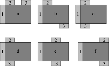
Figure 1: Schematic diagram for the three-terminal setup considered in the present work. The dark shaded region is the central scattering region. The input lead is denoted by lead-1 and the outgoing leads are labeled as lead-2 and lead-3. (a-c) lead-3 is moving away from lead-2. (d-f) Lead-2 and lead-3 are connected symmetrically to the system with respect to lead-1 and are moving away from it.

which depends on the configuration of the system. Here, lead-1 is acting as an input to the system while lead-2 and lead-3 are the outgoing leads. Through lead-1, unpolarized electrons enter into the scattering region and in presence of Rashba spin-orbit interaction, one would expect to observe different kinds of spin species at lead-2 and lead-3 separately. In Fig. 1(a-c), we have fixed the positions of lead-1 and lead-2 and varied the position of lead-3. In Fig. 1(d-f), lead-2 and lead-3 are symmetrically connected to the central scattering region with respect to lead-1.

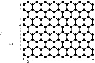
Figure 2: Real view of the central scattering region for calculating the spintronic properties. Edge passivated scenario is not considered here. Leads are not shown here for the better understanding to calculate the dimension of the central scattering region.

The length and width of the system are measured in the conventional way as shown in Fig. 2. Along the $x$-direction, the system has a zigzag shape and along the $y$-direction it is armchair. Hence the system can be defined as $mZ-nA$. The length and width of the ribbon can be calculated as in the following,

$$L_{x}=\frac{\sqrt{3}}{2}(m-1)a,\quad L_{y}=\left(\frac{3}{2}n-1\right)a$$ (1)

where $a=0.142$ nm. Moreover, since we are attaching the outgoing leads at the transverse edges of the central scattering region at different locations, we have not considered the dangling bonds at the edges and therefore any passivated scenario is absent in this work.

The model quantum system is simulated by a tight-binding model, and in presence of Rashba SO coupling the Hamiltonian reads as km1 ; km2 ,

$$H=-t\sum\limits_{\langle ij\rangle}c_{i}^{\dagger}c_{j}+i\alpha\sum\limits_{\langle ij\rangle}c_{i}^{\dagger}\left(\vec{\sigma}\times{\bf\hat{d}}_{ij}\right)_{z}c_{j}$$ (2)

where $c_{i}^{\dagger}=\left(c_{i\uparrow}^{\dagger}\quad c_{i\downarrow}^{\dagger}\right)$. $c_{i\sigma}^{\dagger}$ $(\sigma=\uparrow,\downarrow)$ is the creation operator of an electron at site $i$ with spin $\sigma$. The first term is the nearest-neighbor hopping term, with a hopping strength $t$. The second term is the nearest-neighbor Rashba term which explicitly violates $z\rightarrow-z$ symmetry. $\vec{\sigma}$ denotes the Pauli spin matrices and $\alpha$ is the Rashba SO coupling strength. ${\bf\hat{d}}_{ij}$ is the unit vector that connects the nearest-neighbor sites $i$ and $j$.

The total transmission coefficient, $T_{mn}$, which describes the total transmission probability of electrons from lead $m$ to lead $n$ can be calculated via caroli ; Fisher-Lee ; dutta ,

$$T_{mn}=\rm{Tr}\left[\Gamma_{m}{\cal G}_{R}\Gamma_{n}{\cal G}_{A}\right]$$ (3)

where ${\cal G}_{R(A)}$ is the retarded (advance) Green’s function. $\Gamma_{m(n)}$ are the coupling matrices representing the coupling between the central region and the $m(n)$-th lead.

Finally, the spin-polarized transmission coefficient, $P^{\alpha}_{mn}$, which describes the spin-polarized transmission of electrons that are polarized in a particular direction, $\alpha$ from lead $m$ to lead $n$, can be calculated using chang ,

$$P^{\alpha}_{mn}=\rm{Tr}\left[\hat{\sigma}_{\alpha}\Gamma_{m}G_{R}\Gamma_{n}G_{A}\right]$$ (4)

where, $\alpha=x,y,z$ and $\sigma$ denote the Pauli matrices.

III Results and discussion

We set the hopping term $t=2.7$ eV neto . All the energies are measured in units of $t$. Throughout this paper, we have fixed the strength of Rashba coupling strength at $\alpha=0.1$. The dimension of the scattering region in this work is taken as 401Z-60A. By using Eq. 1, the length of the scattering region is $L_{x}=49.2\approx 50$ nm. The width is $L_{y}=12.64$ nm. The width of lead-1 is same as that of the scattering region, that is, $W_{1}=12.64$ nm and has a zigzag shape. The widths of lead-2 and lead-3 ($101Z$) are $W_{2}=W_{3}=12.3$ nm and have the armchair shape. Thus the widths of these three leads are close to each other. The widths of the outgoing leads have been fixed in such a way that they are metallic in nature. For most of our numerical calculations, we have used KWANT kwant .

Throughout this work, the strength of the Rashba SO coupling has been fixed at $\alpha=0.1$ since this value is very close to the experimentally realized data dedcov . The system dimensions have also been kept same. We have checked the plots shown in this work for different values of $\alpha$ and also for different system sizes (shown in the supplemental material), which differ only in magnitude for the total transmission probability or in the spin-polarized transmission. But the qualitative results, specifically the results obtained in Eq. 5 are valid irrespective of the strength of Rashba SO coupling and the system dimension.

We have essentially studied the behavior of total transmission $T_{mn}$ and all the three components of the spin-polarized transmission $P^{\alpha}_{mn}$ in two different scenarios. First, we have fixed the positions of leads 1 and 2, and varied the position of lead-3 (see Fig. 1(a-c)). In the second case, we have attached the leads 2 and 3 symmetrically with respect to lead-1 and varied the positions of leads 2 and 3 simultaneously away from lead-1 (see Fig. 1(d-f)).

Before going into the essential results, let us start with the variation of density of states (DOS) as a function of the Fermi energy which always gives clear picture of the allowed energy zone for electronic transmission. The results are shown in Fig. 3. From the spectrum we can see that it varies continuously and at $E=0$ there is a sharp dip.

Figure 3: (Color online) Density of states (DOS) as a function of the Fermi energy.

Now we focus on the behavior of total transmission probability as a function of the Fermi energy for the first scenario as mentioned above.

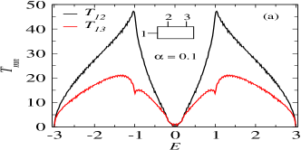
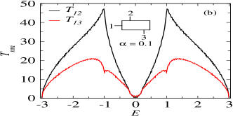
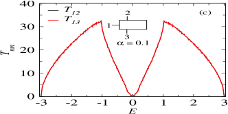
Figure 4: (Color online) Total transmission probability $T_{mn}$ as a function of the Fermi energy. Lead-3 is attached at the (a) extreme top-right (b) extreme bottom-right and (c) extreme bottom-left sides of the central scattering region. The brief setups are shown in the insets of each spectrum.

The results are shown in Fig. 4, where three different cases are considered depending on the specific configurations. The total transmissions $T_{12}$ and $T_{13}$ are denoted by black and red colors respectively. When lead-3 is attached at the top-right (Fig. 1(a)) or at the bottom-right (Fig. 1(b)) side of the central scattering region, both $T_{12}$ and $T_{13}$ show similar behavior as a function of the Fermi energy. This fact indicates that electrons do not see any difference whether lead-3 is connected at the top or bottom of the central scattering region. However, when lead-3 is attached at the bottom-left side of the scattering region, $T_{12}$ and $T_{13}$ become exactly same due to the symmetry of the positions of leads 2 and 3 with respect to lead-1 (Fig. 1(c))as seen from Fig. 4 (c). Under an asymmetric condition, since lead-2 is closer to lead-1 than lead-3, it is clear that most of the carriers from lead-1 will enter into lead-2 and remaining ones will enter into lead-3. As a result, $T_{12}$ will always be higher than $T_{13}$. It is also important to note that, $T_{12}$ is higher for the asymmetric cases (Fig. 4(a) and Fig. 4(b)) than that for the symmetric case (Fig. 4(c)). When lead-2 and lead-3 are connected symmetrically, probabilities of getting electrons at the two outgoing leads are same. Along with this fact, due to the effect of quantum interference among the electronic waves passing through different arms of the junction, $T_{12}$ ($=T_{13}$) for the symmetric case becomes always less than that for the asymmetric one. Moreover, the total transmission spectrum is symmetric about the zero of the Fermi energy similar to that of the DOS spectrum (shown in Fig. 3).

So far, we have studied the total transmission probability for the three-terminal structure in presence of Rashba SO interaction. Let us now study the characteristic features of all the three components of the spin-polarized transmission one by one.

Figures 5(a-c) show the behavior of the $x$-component of the spin-polarized transmission, $P^{x}_{mn}$ as a function of the Fermi energy. All the plots are antisymmetric about the zero of the Fermi energy owing to the particle-hole symmetry of the system.

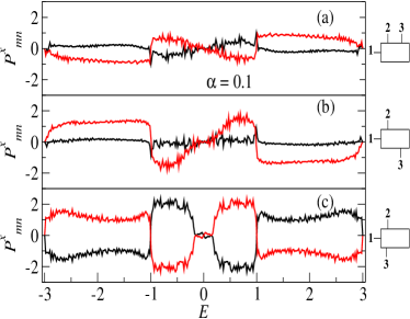
Figure 5: (Color online) $x$-component of spin polarization coefficient, $P^{x}_{mn}$, as a function of the Fermi energy in the two outgoing leads when lead-3 is coupled at the extreme (a) top-right, (b) bottom-right and (c) bottom-left sides of the central scattering region. The black and red colors correspond to the results for lead-2 and lead-3 respectively. The brief setups are shown at the right side of each plot.

The black color denotes the spin-polarized transmission from lead-1 to lead-2 and the red color stands for the same from lead-1 to lead-3. For the first two configurations of the system as shown in Fig. 1(a) and Fig. 1(b), where lead-3 is attached at the top-right and bottom-right side of the central scattering region, $P^{x}_{12}$ does not change much, but this is not the case for $P^{x}_{13}$. In Fig. 5(a) and Fig. 5(b), $P^{x}_{13}$ has opposite signs. For illustration purpose of this feature, let us look into the region $E>0$. In Fig. 5(a), $P^{x}_{13}$ has a negative sign, whereas in Fig. 5(b), it is positive. In presence of Rashba spin-orbit interaction, opposite spins are trying to accumulate in the transverse edges and hence, if more up spins are available at the top side of the sample than the down spin or vice versa, there must be a sign difference in $P^{x}_{13}$ assuming lead-3 is at the top and at the bottom sides of the central scattering region. Another interesting feature can be inferred from Fig. 5(c) when lead-2 and lead-3 are connected symmetrically with respect to lead-1. Here $P^{x}_{12}$ and $P^{x}_{13}$ are antisymmetric to each other.

The sign difference of the spin-polarized transmission in the two outgoing leads has a crucial role in realizing the spin filter device. For example, in Fig. 5(a), $P^{x}_{12}$ and $P^{x}_{13}$ have different signs in the energy region $E<-1\;(E>1)$. The magnitude and sign reversal of spin polarization can be explained from the overlap of the up and and down spin bands. The greater asymmetry between these two spin bands causes higher spin polarization, and when these two bands are completely separated in an energy zone complete polarization can be achieved. Also the sign of the spin polarization depends on which of, that is, up or down energy band dominates. Both the magnitude and the sign of spin polarization depend on the SO coupling strength as well as the position of the leads as directly reflected from Eq. 4. For weak $\alpha$ ($\alpha=0.1$), in the asymmetric case the amplitude will naturally be different as the electronic waves traversing unequal paths before reaching the outgoing leads. Thus a competition ensues between the quantum interference and the SO coupling, and depending on the dominating one both the sign and the magnitude are determined. For higher values of $\alpha$, we see that $P_{12}^{x}$ and $P_{13}^{x}$ exhibit the same sign for the entire energy window which we verify through our extensive numerical analysis (some of these results are also given in the supplemental material). This argument is also valid for the other two components of spin-polarized transmission. Here it is important to note that for the asymmetric lead-to-conductor configuration, it is quite hard to analyze the sign of polarized spin components mathematically. However, for the symmetric configuration these sign issues can be clearly explained with mathematical arguments as discussed below in this work.

The behavior of the $y$-component of the spin-polarized transmission is shown in Fig. 6(a-c) as a function of the Fermi energy.

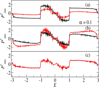
Figure 6: (Color online) $y$-component of spin polarization coefficient, $P^{y}_{mn}$ as a function of the Fermi energy where (a), (b), and (c) correspond to the identical meaning as given in Fig. 5. Different colors represent the identical meaning as described in Fig. 5.

$P^{y}_{12}$ is higher than $P^{y}_{13}$ when lead-2 and lead-3 are attached on the same side of the system as seen from Fig. 6(a). This indicates that lead-2 is picking up more $y$-component of spin than lead-3. However, when lead-3 is at the bottom side of the system, the difference between $P^{y}_{12}$ and $P^{y}_{13}$ become less (Fig. 6(b)) and they are exactly same when lead-2 and lead-3 are connected symmetrically (Fig. 6(c)). Unlike the $x$-component of spin-polarized transmissions, the $y$-component of the spin-polarized transmissions, $P^{y}_{12}$ and $P^{y}_{13}$ behave similar to total transmission in the symmetric case.

The behavior of the $z$-component of the spin-polarized transmission is plotted in Fig. 7(a-c) as a function of the Fermi energy.

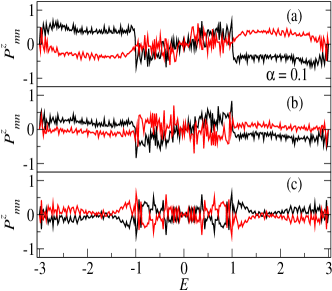
Figure 7: (Color online) $z$-component of spin polarization coefficient, $P^{z}_{mn}$ as a function of the Fermi energy where (a), (b), and (c) correspond to the identical meaning as given in Fig. 5. Different colors represent the identical meaning as described in Fig. 5.

In Fig. 7(a), when lead-2 and 3 are on the same side of the system, $P^{z}_{12}$ is little higher than $P^{z}_{13}$. However, when lead-3 is at the bottom, both the spin-polarized transmissions are reduced as shown in Fig. 7(b). In Fig. 7(c), where lead-2 and lead-3 are symmetrically connected, $P^{z}_{12}$ and $P^{z}_{13}$ are antisymmetric to each other.

Comparing the spectra given in Figs. (5-7) we can see that $P^{x}_{12}$ is higher when the two output leads are connected symmetrically with respect to the input lead than the other two configurations. On the other hand, irrespective of the sign, the variations of $P^{x}_{13}$ for the three different configurations are more or less similar. For the energy region $E<-1$ or $E>1$, $P^{y}_{12}$ gets a higher value when two output leads are on the same side. Again in the same mentioned energy region, the magnitude of $P^{y}_{13}$ is in the descending order for the three configurations, namely when the lead-3 is attached at the bottom-right, bottom-left, and top-right positions. The $z$-component of the spin-polarized transmission, $P^{z}_{12}$ has the highest value when the two output leads are on the same side and have the lowest value for the bottom-left configuration. $P^{z}_{13}$ shows exactly opposite behavior with respect to $P^{z}_{12}$.

Now, we shall focus on the symmetric configurations of the two output leads as shown in Fig. 1(d-f). Here the three different configurations correspond to the cases when the two output leads are symmetrically attached at the extreme left (Fig. 1(d)), middle (Fig. 1(e)) and extreme right (Fig. 1(f)) sides of the central scattering region.

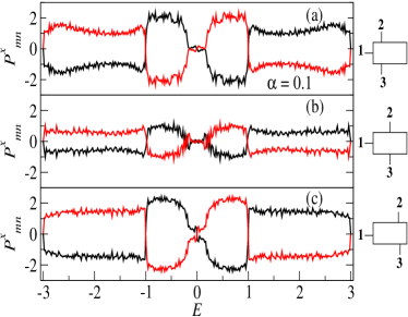
Figure 8: (Color online) $x$-component of spin polarization coefficient, $P^{x}_{mn}$ as a function of the Fermi energy for the symmetric case. The outgoing leads are connected at the (a) extreme left, (b) middle and (c) extreme right sides of the central scattering region. Different colors represent the identical meaning as described in Fig. 5. The brief setups are shown at the right side of each plot.

In all those setups, the two symmetrically coupled output leads are positioned away from the input lead and want to study if there is any effect on the distance between the input and output leads on the spin-polarized transport properties.

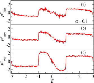
Figure 9: (Color online) $y$-component of spin polarization coefficient, $P^{y}_{mn}$ as a function of the Fermi energy where (a), (b), and (c) correspond to the identical meaning as given in Fig. 8. Different colors represent the identical meaning as described in Fig. 5.

The characteristic features of $P^{\alpha}_{12}$ and $P^{\alpha}_{13}$ as a function of the Fermi energy are shown in Fig. 8, Fig. 9 and Fig. 10. The black lines denote the results for the output lead-2, while for the other lead (lead-3), the results are presented by the red lines. From the behavior of the spin-polarized transmissions, it is observed that the $x$ and $z$-components of the spin-polarized transmission in two symmetrically coupled output leads carry

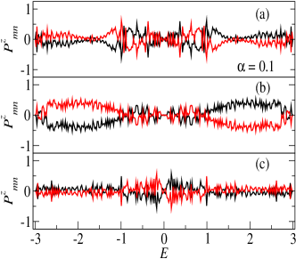
Figure 10: (Color online) $z$-component of spin polarization coefficient, $P^{z}_{mn}$ as a function of the Fermi energy where (a), (b), and (c) correspond to the identical meaning as given in Fig. 8. Different colors represent the identical meaning as described in Fig. 5.

opposite signs as a function of the Fermi energy. In other words, $P^{\alpha}_{12}$ and $P^{\alpha}_{13}$ ($\alpha\in x,z$) are antisymmetric to each other. On the other hand, the $y$-components in two symmetrically coupled output leads are exactly same as a function of the Fermi energy. These features are explained in the following arguments from the point of view of the structural symmetry of the system. Moreover, the overall magnitude of the $x$-component is lower for the configuration in which the two outgoing leads are placed at the middle of the central scattering region than the other two configurations. This is entirely due to the quantum interference among the electronic waves flowing through the output leads. When the two output leads are at either extremes of the central scattering region, the constructive interference dominates compared to the case where the two outgoing leads are placed at the middle.

The systems described in Fig. 1(d-f) are symmetric with respect to the reflection $y\rightarrow-y$ kim-jap . This mirror-symmetry of the $y$-axis has an effect on the S-matrix elements, and by analyzing the S-matrix symmetry Kiselev et al. kim-jap have shown analytically that in a T-shaped conductor in presence of SO interaction, the transmission amplitudes for the $x$ and $z$ components have equal magnitude and opposite phases for symmetrically connected output leads. While, the $y$-component has identical phase in the output leads with equal magnitude. Thus we can summarize our observations in a compact way as,

$$\left.\begin{aligned} T_{12}(E)&=&T_{13}(E)\\ P^{x}_{12}(E)&=&-P^{x}_{13}(E)\\ P^{y}_{12}(E)&=&P^{y}_{13}(E)\\ P^{z}_{12}(E)&=&-P^{z}_{13}(E)\end{aligned}\right\}$$ (5)

Further, from Fig. 10, it is noted that the $z$-component of the spin-polarized transmission is much lower than the other two components (approximately 3 times). Moreover, the values of the $x$ and $y$ components are relatively close to each other.

IV Conclusion

To conclude, in the present work, we have studied spin dependent transport through a three-terminal GNR in presence of Rashba SO interaction exploiting the effect of quantum interference among the electronic waves passing through different arms of the junction. The three-terminal structure aides in generating all the three components of the spin-polarized transmission ($P_{x}$, $P_{y}$ and $P_{z}$) which was not feasible in a two-terminal GNR and hence it can be used as an efficient spin filter device compared to a two-terminal one. In addition to that, those spin-polarized transmissions can be obtained simultaneously through the two outgoing leads in a three-terminal device. Thus, more spin operations are performed simultaneously which would not have been possible for a setup with only one outgoing lead. Two different scenarios have been considered. First we have fixed one outgoing lead (lead-2) and moved the other outgoing lead (lead-3) away from the other and in this case, we have an asymmetric geometry. The second scenario is based on the symmetric configuration of the system, where two leads are attached symmetrically to the system with respect to the input lead (lead-1). The $x$ and $z$-components of the spin-polarized transmission have higher values for the symmetric case, whereas the total transmission $T$ and the $y$-component of the spin-polarized transmission are higher corresponding to the case when both the outgoing leads are on the same side than the other configurations of the system. Moreover, since the $x$ and $z$-components of the spin-polarized transmission have the opposite signs in two symmetrically coupled output leads as a function of the Fermi energy, the symmetric setup can be used as a switching device.

The main text discusses the spintronic properties of a three-terminal graphene nanoribbon (GNR) in presence of Rashba spin-orbit coupling, where all the results have been computed considering the Rashba coupling strength $\alpha=0.1$ and the dimension of the central scattering region as 401Z-60A. The width of lead-1 is same as that of the scattering region, that is, 60A and that of lead-2 and lead-3 are both 101Z. In this supplementary material we have shown results for density of states (DOS), total transmission coefficient and the three components of the spin-polarized transmission ($P_{x}$, $P_{y}$ and $P_{z}$) for different values of $\alpha$ and for different dimensions of the

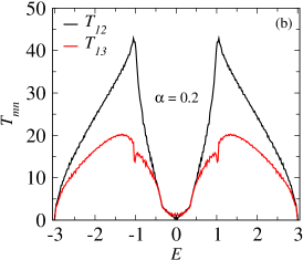
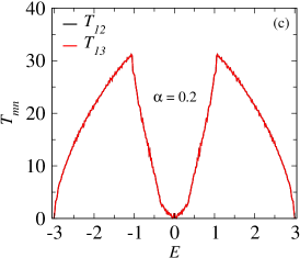
Figure S1: (Color online) (a) Density of states (DOS) as a function of the Fermi energy. Transmission coefficients as a function of the Fermi energy for (b) asymmetric configuration corresponding to Fig.1(a) in the main paper and (c) symmetric configuration corresponding to Fig.1(e) in the main paper. The Rashba spin-orbit coupling strength is $\alpha=0.2$. The black and red colors represent the results for lead-2 and lead-3 respectively.

central scattering region. Here the dimension of the scattering region in Fig. S1 and Fig. S2 is taken as 601Z-60A and that in Fig. S3 and Fig. S4 as 801Z-60A. The widths of the leads are kept same as in the main paper.

The DOS as a function of the Fermi energy is shown in Fig. S1(a) for the Rashba coupling strength $\alpha=0.2$. If we compare the DOS here and the corresponding plot as given in Fig. 3 of the main paper, we see that both DOS have more or less similar behavior as a function of $E$, though the strengths of the Rashba coupling are different (in the main text, $\alpha=0.1$).

The total transmission probability amplitudes in the two outgoing leads are presented as a function of the Fermi energy for $\alpha=0.2$ in Figs. S1(b) and (c). Here we have considered only two configurations of the system, that is, an asymmetric configuration (Fig.1(a) in the main paper) and a symmetric configuration (Fig.1(e) in the main paper) as shown in Figs. S1(b) and (c), respectively in this supplemental material. For the asymmetric case, where two outgoing leads are on the same side of the central scattering region, $T_{12}$ is greater than $T_{13}$ (defined in the main text) and this feature is exactly same with the transmission spectra for $\alpha=0.1$ and also for a different dimension of the central scattering region. Further, the symmetric configuration shows similar behavior as discussed in the main paper, that is, $T_{12}$ and $T_{13}$ remain exactly identical.

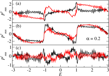
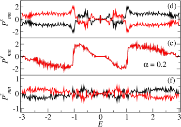
Figure S2: (Color online) $P_{x}$, $P_{y}$ and $P_{z}$ as a function of the Fermi energy for two different configurations, where the left and right columns correspond to the cases as used in Fig. S1(b) and Fig. S1(c) respectively. The Rashba spin-orbit coupling strength $\alpha$ is fixed at 0.2. The black and red colors represent the outputs for lead-2 and lead-3 respectively.

The three components of the spin-polarized transmission, $P_{x}$, $P_{y}$ and $P_{z}$ are given as a function of the Fermi energy both for the asymmetric (results are shown in Fig. S2(a-c)) and symmetric cases (results are shown in Fig. S2(d-f)). The strength of the Rashba coupling and the system dimension are same as in Fig. S1. The qualitative features of the spin-polarized transmission spectra are similar to the features discussed in the main paper.

The DOS for a higher value of $\alpha=0.5$ and also corresponding to a higher dimension (601Z-60A) is shown in Fig. S3(a) as a function of the Fermi energy which has similar behavior as observed in Fig. S1(a). The total transmission probability amplitudes in the two outgoing leads as a function of the Fermi energy are shown in Fig. S3(b) for the asymmetric case and in Fig. S3(c) for the symmetric case. These plots have similar features as we have discussed earlier for the other values of Rashba coupling strength and for different dimensions of the system.

In Fig. S4, the variations of $P_{x}$, $P_{y}$ and $P_{z}$ are presented as a function of the Fermi energy for the same parameters as used in Fig. S3. Owing to the higher value of $\alpha$ (=0.5) ,

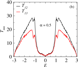
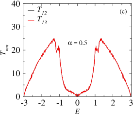
Figure S3: (Color online) (a) Density of states (DOS) as a function of the Fermi energy. Transmission coefficients as a function of the Fermi energy for (b) asymmetric configuration and (c) symmetric configuration as used in Fig. S1(b) and Fig. S1(c) respectively. The Rashba spin-orbit coupling strength is $\alpha=0.5$. Different colors represent the identical meaning as described in Fig. S1.

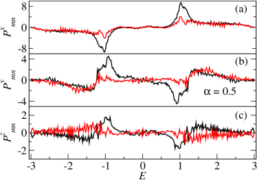
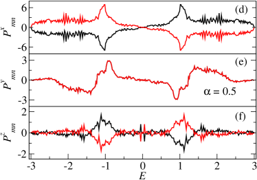
Figure S4: (Color online) $P_{x}$, $P_{y}$ and $P_{z}$ as a function of the Fermi energy for two different configurations, where the left and right columns correspond to the cases as used in Fig. S1(b) and Fig. S1(c) respectively. The Rashba spin-orbit coupling strength $\alpha$ is fixed at 0.5. Different colors represent the identical meaning as described in Fig. S2.

the magnitude of the spin-polarized transmission is greater than the previous cases. However, the qualitative features remain independent of the value of the Rashba coupling strength and the system dimensions. Thus, we can strongly argue that the results presented here are valid for a wide range of parameter values which prove the robustness of our analysis. We believe that the studied results will bring significant impact in analyzing selective spin transmission through multi-terminal systems comprising different topological systems.