Formal Solutions for Polarized Radiative Transfer
IV. Numerical Performances in Practical Problems

Abstract

The numerical computation of reliable and accurate Stokes profiles is of great relevance in solar physics. In the synthesis process, many actors play a relevant role: among them the formal solver, the discrete atmospheric model, and the spectral line. This paper tests the performances of different numerical schemes in the synthesis of polarized spectra for different spectral lines and atmospheric models. The hierarchy between formal solvers is enforced, stressing the peculiarities of high-order and low-order formal solvers. The density of grid points necessary for reaching a given accuracy requirement is quantitatively described for specific situations.

1. Introduction

Polarization is a property of light that encodes a wealth of information about the physical state of the environment from which the light emerges, making the radiative transfer of polarized light a topic of great interest in remote sensing. The usual differential form of the radiative transfer equation of partially polarized light reads

$$\frac{\rm d}{{\rm d}s}\mathbf{I}(s)=-\mathbf{K}(s)\mathbf{I}(s)+\bm{\epsilon}(s)\,.$$ (1)

It is a system of first-order coupled inhomogeneous ordinary differential equations, where $\mathbf{I}=(I,Q,U,V)^{T}$ is the Stokes vector, $\mathbf{K}$ is the $4\times 4$ propagation matrix, and $\bm{\epsilon}$ is the emission vector. All of these quantities depend on the spatial coordinate $s$ measured along the ray under consideration. To simplify the notation, the frequency dependence of these quantities is omitted.

Equation (1) seldom has solutions that can be expressed in an analytical form, so it is common to seek approximate solutions by means of numerical methods. The so-called formal solution of Equation (1) consists of the numerical evaluation of the Stokes vector, given knowledge of the propagation matrix and the emission vector at a discrete set of spatial points and of the boundary conditions (Auer, 2003).

In the general nonlinear problem, the emission vector and the propagation matrix depend on the Stokes vector. In this case, the formal solution is supplemented by the statistical equilibrium equations or by redistribution matrices for scattering processes. The whole problem is usually solved iteratively involving a large number of formal solutions per single iteration (Trujillo Bueno, 2003; Landi Degl’Innocenti & Landolfi, 2004). Another issue of growing importance is the massive Stokes profiles synthesis on atmosphere models from 3D radiative-magnetohydrodynamic (R-MHD) simulations. Moreover, inversion techniques require repetitive evaluation of Equation (1) (Bellot Rubio et al., 2000; del Toro Iniesta & Ruiz Cobo, 2016).

These computationally demanding problems call for an efficient and accurate integration of Equation (1), in which the crucial role of the formal solver is well recognized. For this reason, Janett et al. (2017b, a) characterized formal solvers in terms of order of accuracy, stability, and computational cost. Furthermore, Janett & Paganini (2018) analyzed the stiffness of the radiative transfer equation of polarized light, identifying the instability issues and outlining the structure of pragmatic numerical schemes. In practice, the discrete atmospheric model also plays a fundamental role in the formal solution. On the one hand, most of formal solvers achieve satisfying accuracy when considering finely sampled smooth model atmospheres. On the other hand, most of formal solvers notoriously fail on intermittent atmospheric models with coarse spatial grids. The debate on the optimal formal solution for polarized light is definitely not over.

Section 2 describes the usual contexts of numerical syntheses of Stokes profiles. Section 3 presents a selected pool of numerical schemes for the numerical integration of Equation (1). Section 4 focuses on selected atmospheric models, paying particular attention to their sampling in terms of density of spatial grid points. Section 5 exposes numerical tests for different cases. Finally, Section 6 provides remarks and conclusions.

2. Physics

Many practical applications of radiative transfer for polarized radiation in solar and stellar atmospheres concern the problem of line formation in the presence of a magnetic field (Landi Degl’Innocenti & Landolfi, 2004). There are various ingredients that can modify the inputs of the formal solution, i.e., the propagation matrix and emission vector coefficients at the different grid points and their relative spacing. This section provides a brief overview on the most important physical aspects in which the formal solutions generally differ.

2.1. Spectral line

Spectral lines originate from very different atomic transitions that are differently sensitive to atmospheric physical conditions (del Toro Iniesta & Ruiz Cobo, 2016). Solar spectral lines are usually analyzed to determine the conditions of the atmospheric regions in which they are formed, hence the distinction between photospheric, chromospheric, transition region, and coronal spectral lines. In fact, a spectral line samples a range of geometrical heights, which usually increase from the line wings to the line center. The relative contribution of an atmospheric layer to an observed quantity is generally quantified using contribution functions (Magain, 1986; Grossmann-Doerth et al., 1988), while response functions provide information about how changes in the atmospheric parameters modify the emergent Stokes spectrum (Grossmann-Doerth et al., 1988; Ruiz Cobo & del Toro Iniesta, 1992; Bellot Rubio et al., 1998).

In this work, calculations are carried out for different spectral lines forming in photospheric and chromospheric regions. Table 1 gives for each considered atomic transition the central wavelength, $\lambda_{0}$, and the Einstein coefficient, $A_{ul}$. Figure 1 shows the height at which the line center optical depth is equal one for the selected spectral lines and atmospheric model.

Table 1Spectral lines

Ion	Transition	$\lambda_{0}[{\rm\mbox{\AA}}]$	$A_{ul}[s^{-1}]$
Sr i	${}^{1}S_{0}\,-\,^{1}P_{1}$	4607.3	2.01$\,\times\,10^{8}$
Fe i	${}^{5}P_{2}\,-\,^{5}D_{2}$	6301.5	7.14$\,\times\,10^{6}$
Fe i	${}^{5}P_{1}\,-\,^{5}D_{0}$	6302.4	1.24$\,\times\,10^{7}$
Ba ii	${}^{2}S_{1/2}\,-\,^{2}P_{3/2}$	4554.0	1.11$\,\times\,10^{8}$
Ca ii	${}^{2}D_{5/2}\,-\,^{2}P_{3/2}$	8542.1	9.90$\,\times\,10^{6}$
Ca ii K	${}^{2}S_{1/2}\,-\,^{2}P_{3/2}$	3933.6	1.47$\,\times\,10^{8}$
Mg ii k	${}^{2}S_{1/2}\,-\,^{2}P_{3/2}$	2795.5	2.60$\,\times\,10^{8}$

2.2. LTE versus NLTE

The propagation matrix coefficients and the emission vector components in Equation (1) are usually functions of the level population densities and other atmospheric physical parameters: among them the temperature, the microscopic and macroscopic velocities, and the strength and orientation of the magnetic field. Under the assumption of local thermodynamic equilibrium (LTE), the level population densities are defined by the local temperature only and decoupled from the radiation field. The assumption of LTE conditions satisfactorily describes the formation of many photospheric spectral lines. For lines forming higher up in the solar atmosphere, however, this assumption must be abandoned. This happens, for instance, in the presence of low collisional rates, where the atomic system and the radiation field interact in non-local thermodynamic equilibrium (NLTE) conditions. NLTE conditions imply that the emission vector and the propagation matrix depend in a complicated manner on the Stokes vector, so that Equation (1) is nonlinear and the formal solution is supplemented by additional statistical equilibrium equations and/or by suitable redistribution matrices for scattering processes.

In this work, the LTE and NLTE conditions are assumed for the synthesis of photospheric and chromospheric lines, respectively. NLTE effects are included in terms of the field-free approximation (Rees, 1969), where the statistical equilibrium equations for the level populations are solved as if the magnetic field was absent.

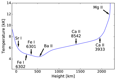
Figure 1.— Formation heights for the spectral lines given in Table 1 in the FALC atmospheric model. Arrows indicate the height at which the line center optical depth is equal to unity.

2.3. Dimensionality

It is known that “once the assumption of LTE is abandoned, the dimensionality of the atmosphere comes into play, since the non-locality of the radiation field manifests itself in the vertical, as well as in the horizontal dimensions” (de la Cruz Rodríguez & van Noort, 2017). Mihalas et al. (1978) and, subsequently, Kunasz & Auer (1988) presented the difficulties inherent to the solution of unpolarized radiative transfer in 2D slab geometries. Stenholm & Stenflo (1977) pioneered calculations of multidimensional transfer of the Stokes vector in magnetic fluxtubes. More recently, Štěpán & Trujillo Bueno (2013) published PORTA, a code able to solve the non-equilibrium problem of the generation and transfer of polarized radiation in 3D solar atmospheres.

For 1D problems, the grid points lay on the unique ray under consideration. However, for 2D or 3D problems, the ray path (long characteristics) or the downwind and upwind points (short characteristics) do not generally coincide with the grid points. In this case, one must recover the relevant quantities at off-grid points typically through interpolation (or reconstruction). Such interpolations may introduce numerical errors in the absorption and emission coefficients. Moreover, the cell widths of redefined discretized path may become highly irregular (e.g., Mihalas et al., 1978).

Since Equation (1) is always numerically integrated along a ray, the dimensionality of the grid enters the formal solution only when determining downwind and upwind quantities (Auer, 2003). Therefore, without any limitation to the analysis of formal solvers, the 1D geometry is always adopted in Section 5.

2.4. Polarizing mechanisms

Polarization is introduced in spectral lines by several different symmetry-breaking mechanisms that are connected either to the presence of an external field, e.g, the magnetic field, or to some kind of anisotropy in the excitation of the atomic system, e.g., the optical pumping (Landi Degl’Innocenti & Landolfi, 2004). The magnetic field influences the polarization of the emergent radiation in different ways, which depend on details of the atomic physics. A common distinction is made between the Zeeman or Paschen-Back effects and the Hanle effect, which have different sensitivities to the strength and orientation of the magnetic field. In the Stokes syntheses of this work, the polarization of spectral lines is produced by the Zeeman effect alone.

2.5. Spatial scale

Janett & Paganini (2018) demonstrated that the stiffness of Equation (1) is spatial scale dependent. The conversion to the optical depth scale given by

$$\tau(s)=\tau_{0}+\int_{s_{0}}^{s}\eta_{I}(x)\,{\rm d}x\,,$$ (2)

where $\eta_{I}$ is the intensity absorption coefficient at the frequency under consideration, recasts Equation (1) into the equivalent form

$$\frac{\rm d}{\rm d\tau}\mathbf{I}(\tau)=-\tilde{\mathbf{K}}(\tau)\mathbf{I}(\tau)+\tilde{\bm{\epsilon}}\,,$$

where $\tilde{\mathbf{K}}=\mathbf{K}/\eta_{I}$ and $\tilde{\bm{\epsilon}}=\bm{\epsilon}/\eta_{I}$. The use of the optical depth scale (instead of the geometrical scale) usually mitigates variations of the entries of the propagation matrix along the ray path, damping instability issues. Figure 2 presents some numerical evidence, showing the unstable (stable) behavior of the cubic Hermitian method when using the geometrical (optical) depth scale on very coarse spatial grids. Note that the conversion to the optical depth scale requires the quadrature of the integral in Equation (2) and introduces numerical errors. These errors might reduce the order of accuracy of the formal solver and even lead to instabilities issues.

For the sake of clarity, calculations in Section 5 are carried out in the optical depth scale given by Equation (2) at the frequency under consideration (with the exception of the pragmatic formal solvers). High-order numerical schemes are always combined with corresponding order monotonic spatial scale conversion: trapezoidal rule for second-order schemes and interpolatory quadrature rules for third-order (based on Fritsch & Butland, 1984) and forth-order (based on Steffen, 1990) methods.

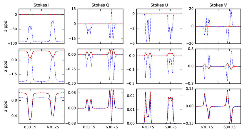
Figure 2.— Emerging Stokes vector components for the Fe i spectral lines at 6301.5 and 6302.5 Å in the FALC atmospheric model presented in Figure 3. The Stokes profiles are calculated with the cubic Hermitian method in the geometrical depth scale (dashed blue) and in the optical depth scale (dashed red) for different spatial point densities. The reference emergent Stokes profile (continuous black) is calculated using a sampling with $10^{3}$ points-per-decade (ppd) of continuum optical depth. The dashed red and solid black lines almost overlap. Note the variations in the $y$-axis scale among the different plots.

3. Formal solvers

For the sake of clarity, only a limited number of numerical schemes is analyzed. However, the numerical tests performed in Section 5 can be unconditionally applied to any formal solver. This section presents a pool of candidate numerical schemes selected according to three criteria: order of accuracy, numerical stability, and computational cost. Table 2 gives a short overview of such schemes.

Table 2Numerical schemes

Formal solver	Order	Stability	Time cost
Heun’s	2	-	2.51$\times 10^{-7}$
Trapezoidal	2	$A$-stable	8.40$\times 10^{-7}$
DELO-linear	2	$L$-stable	9.65$\times 10^{-7}$
Runge-Kutta 3	3	-	3.83$\times 10^{-7}$
Adams-Moulton 3	3	-	1.05$\times 10^{-6}$
DELO-parabolic	3	$L$-stable8	1.15$\times 10^{-6}$
cubic Hermitian	4	$A$-stable	1.15$\times 10^{-6}$
quadratic DELO-Bézier	4	$L$-stable8	1.35$\times 10^{-6}$
cubic DELO-Bézier	4	$L$-stable8	1.40$\times 10^{-6}$

3.1. Trapezoidal method

The well-known implicit trapezoidal method is an optimal representative of low-order implicit formal solvers. It is second-order accurate and $A$-stable (i.e., its stability region comprises the complex left half-plane $\mathbb{C}^{-}$). Moreover, it consists of a skeletal algorithm. Janett et al. (2017b) gave a detailed description of the method and its application to Equation (1).

3.2. Adams-Moulton 3 method

The Adams-Moulton 3 method is an implicit linear two-step method and it is third-order accurate. It suffers from numerical instability when treating optically thick cells because of its bounded stability region (Janett et al., 2017a). Moreover, the effect of variable cell size on the stability of multistep methods is not fully understood and might be relevant for radiative transfer applications. A deeper look into this problem is given by Geart & Tu (1974) and Grigorieff (1983).

3.3. Cubic Hermitian method

Bellot Rubio et al. (1998) first proposed the cubic Hermitian method for the integration of Equation (1). Janett et al. (2017a) subsequently reaffirmed the excellence of this implicit method in terms of accuracy and stability: it is fourth-order accurate and $A$-stable. A possible weakness of this method could lay in its complexity. In fact, it requires matrix-by-matrix multiplications and, in particular, the calculation of second-order accurate numerical derivatives appears to be the most expensive part of the method.

Moreover, Ibgui et al. (2013) explained that the calculation of numerical derivatives proposed by Steffen (1990) is sensibly slower than the one proposed by Fritsch & Butland (1984). However, the derivatives provided by Fritsch & Butland (1984) are second-order accurate on uniform grids only and they drop to first-order accuracy on non-uniform grids (see Janett & Paganini, 2018). For this reason, the version by Steffen (1990) is used here.

3.4. DELO-linear

The popular DELO-linear implicit formal solver linearly approximates the effective source function (see Rees et al., 1989) guaranteeing second-order accuracy. Thanks to its proximity to $L$-stability, it avoids instability issues and correctly replicates exponential attenuations even when the step-size is large (Janett & Paganini, 2018).

3.5. DELO-parabolic

The DELO-parabolic implicit method approximates the effective source function with a parabola, resulting in a third-order accurate two-step method (Janett et al., 2017b). There exist contradicting opinions on its stability properties: Murphy (1990) mentioned the numerical instability due to the parabolic approximation (overshooting), while Janett & Paganini (2018) demonstrated its proximity to $L$-stability. Similarly as for the Adams-Moulton 3 method, the effect of variable cell size might be relevant for stability issues.

3.6. Quadratic and cubic DELO-Bézier methods

The quadratic and cubic DELO-Bézier methods are implicit schemes based on quadratic and cubic Bézier approximations of the effective source function, respectively (de la Cruz Rodríguez & Piskunov, 2013). Providing at least second-order accurate derivatives, both methods can reach fourth-order accuracy. Janett & Paganini (2018) demonstrated their proximity to $L$-stability. Similarly to the cubic Hermitian method, DELO-Bézier methods require the calculation of numerical derivatives that increases the total computational effort. For the same arguments given in Section 3.3, the calculation of numerical derivatives proposed by Steffen (1990) is preferred here.

3.7. Second-order pragmatic method

Janett & Paganini (2018) suggested considering each integration interval at a time and sequentially. In each interval, depending on the cell width $\Delta s$ and on the eigenvalues of $\mathbf{K}$ at the cell boundaries, the Stokes vector is calculated with either an explicit method $\mathbf{\Psi}^{E}$ (which is computationally cheaper) or an $A$-stable method $\mathbf{\Psi}^{A}$, or an $L$-stable method $\mathbf{\Psi}^{L}$.

The second-order pragmatic method proposed here uses Heun’s method as $\mathbf{\Psi}^{E}$, the implicit trapezoidal method as $\mathbf{\Psi}^{A}$, and the DELO-linear method as $\mathbf{\Psi}^{L}$. Both Heun’s method and the implicit trapezoidal method use the geometrical spatial scale. The method $\mathbf{\Psi}^{E}$ is used if the stability function $\phi_{\mathbf{\Psi}^{E}}$ satisfies $\phi_{\mathbf{\Psi}^{E}}<0.95$ or if $\Delta\tau<10^{-3}$; alternatively, the method $\mathbf{\Psi}^{A}$ is used if $\phi_{\mathbf{\Psi}^{A}}<1.0$ (see Janett & Paganini, 2018, Sect. 6). Otherwise, or whenever $\Delta\tau>7$, the method $\mathbf{\Psi}^{L}$ is used, guaranteeing numerical stability and the correct exponential attenuation of the Stokes vector. These parameters should not be considered as an ultimate choice, but they provide accurate and stable numerical results. Algorithm 1 in Appendix A presents the pseudocode of the method.

The overhead caused by the first switching decision is roughly half as expensive as one step of Heun’s method. Moreover, the use in percentage of $\mathbf{\Psi}^{E}$, $\mathbf{\Psi}^{A}$, and $\mathbf{\Psi}^{L}$ depends on the atmospheric model and on the density of grid points (see Janett & Paganini, 2018, Table 2). For these reasons, the pragmatic method is particularly competitive when it performs many steps with $\mathbf{\Psi}^{E}$, but it looses efficiency when using many $\mathbf{\Psi}^{A}$ and $\mathbf{\Psi}^{L}$ steps, i.e., in very coarse grids.

3.8. Third-order pragmatic method

The pragmatic strategy by Janett & Paganini (2018) is extensible to higher order. For instance, the third-order pragmatic method proposed here uses the explicit RK 3 method as $\mathbf{\Psi}^{E}$ (e.g., Hairer et al., 2000), the third-order Hermitian method as $\mathbf{\Psi}^{A}$, and the DELO-linear method as $\mathbf{\Psi}^{L}$. Both the RK 3 method and the third-order Hermitian method use the geometrical spatial scale. The method $\mathbf{\Psi}^{E}$ is used if the stability function $\phi_{\mathbf{\Psi}^{E}}$ (Frank & Leimkuhler, 2012) satisfies $\phi_{\mathbf{\Psi}^{E}}<0.95$ or if $\Delta\tau<10^{-3}$; alternatively, the method $\mathbf{\Psi}^{A}$ is used if $\phi_{\mathbf{\Psi}^{A}}<1.0$ (see Janett et al., 2017a). Otherwise, or whenever $\Delta\tau>10$, the method $\mathbf{\Psi}^{L}$ is used, guaranteeing numerical stability and the correct exponential attenuation of the Stokes vector. Algorithm 2 in Appendix A presents the pseudocode of the method.

The computational efficiency of this method is analogous to that of the second-order pragmatic method.

4. Atmospheric models

Radiative transfer problems are usually solved for discrete atmospheric models, where the physical quantities describing the atmosphere are given at a discrete set of spatial points. The propagation matrix and emission vector coefficients are then calculated at grid points, allowing the numerical integration of Equation (1).

Equation (1) is usually solved on the atmospheric model grid. However, one can still add, move, or remove grid points: this is usually done through interpolation and by cutting off irrelevant atmospheric layers. It is certainly not possible to state the minimal amount of grid points necessary to achieve a certain accuracy because an atmosphere sampling giving satisfactory results for one specific spectral line may produce large errors for another one formed at a different depth and range. Clearly, it is self-defeating to distribute spatial grid points too deep in the solar atmosphere, where the exponential attenuation cancels any contribution to the emergent spectrum. When considering the homogeneous version of Equation (1) in the limit of a vanishing magnetic field, one has

$$\mathbf{I}(\tau)\approx e^{-\Delta\tau}\mathbf{I}(\tau_{0})\,,$$

where $\Delta\tau=|\tau-\tau_{0}|$. This exponential attenuation guarantees that an optically thick layer, say, $\Delta\tau\geq 20$, cancels any relevant contribution of the incoming light to the emergent spectrum. A quantitative perception of the exponential attenuation is given in Table 3.

When analyzing the performances of formal solvers, it is common to choose a homogeneous sampling in $\log\tau_{c}$ (e.g., Rees et al., 1989; Bellot Rubio et al., 1998; de la Cruz Rodríguez & Piskunov, 2013), where the coordinate $\tau_{c}$ is the continuum optical depth defined by

$${\rm d}\tau_{c}=-\eta_{c}(s){\rm d}s\,,$$

with $\eta_{c}$ being the continuum absorption coefficient at the wavelength $\lambda=5000$ Å. One then defines the quantity of points-per-decade (ppd) of $\tau_{c}$, indicating the amount of grid points that sample a variation of one order of magnitude in the continuum optical depth. Therefore, one speaks of the grid-point density (ppd) rather than referring to the total amount of grid points.

In order to analyze the accuracy of the formal solution as a function of the cell width, one needs a sequence of discrete grids with an increasing (or decreasing) grid-point density. In this work, the following procedure is used: first, the original discrete atmospheric model is interpolated in terms of cubic splines in each quantity. Second, the run of the atmospheric parameters is restricted to a specific interval in continuum optical depth (e.g., $\log\tau_{c}\in[-8,2]$). Third, a sequence of models with increasing grid-point densities is generated.

In the following, three different atmospheric model categories are presented: analytical, semi-empirical, and 3D R-MHD atmospheric models.

Table 3Exponential attenuation

Optical width $\Delta\tau$	$\log\Delta\tau$	Attenuation factor $e^{-\Delta\tau}$
1	0.0	0.36
5	0.7	6.7$\times 10^{-3}$
10	1.0	4.5$\times 10^{-5}$
20	1.3	2.0$\times 10^{-9}$
50	1.7	1.9$\times 10^{-22}$
100	2.0	3.7$\times 10^{-44}$

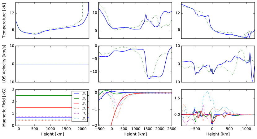
Figure 3.— Temperature (top row), upward directed line of sight velocity (middle row), three components of the magnetic field (bottom row), all as a function of the geometrical height in the atmosphere. Considered atmospheric models: first column FALC (solid), FALF (dotted); second column Bifrost-1 (solid), Bifrost-2 (dotted); third column CO⁵BOLD-1 (solid), CO⁵BOLD-2 (dotted). Note that Bifrost-1, Bifrost-2, CO⁵BOLD-1, and CO⁵BOLD-2 are single columns of time instants of 3D R-MHD simulations.

4.1. Analytical atmospheric models

A great number of attempts have been made to obtain exact solutions of the polarized radiative transfer equation using analytical atmospheric models. The best-known case is the so-called Milne-Eddington atmospheric model. This model implies LTE conditions, a constant propagation matrix, and that the Planck function varies linearly with optical depth. Unno (1956) first provided the solution of Equation (1) for a Milne-Eddington atmosphere with vanishing magneto-optical effects, and Rachkovsky (1967) subsequently gave the complete solution. Thereafter, Landi Degl’Innocenti (1987) analytically solved Equation (1) in terms of the evolution operator for different cases, where both the propagation matrix and the emission vector are given functions of the optical depth. In addition, López Ariste & Semel (1999) propose an alternative strategy to analytically handle different cases with a non-constant propagation matrix. Moreover, analytical atmospheric models have been frequently used to test the performances of various formal solvers (e.g., Bellot Rubio et al., 1998; Štěpán & Trujillo Bueno, 2013). In particular, Janett et al. (2017b, a) tested different formal solvers using an analytically prescribed model atmosphere. To avoid superfluous repetitions, no analytical atmospheric model is considered in this work.

4.2. Semi-empirical atmospheric models

Semi-empirical models assume a 1D atmosphere in hydrostatic equilibrium with a temperature structure, so as to reproduce various mean diagnostic quantities of the atmosphere, averaging both temporally and spatially (Mauas, 2007).

There exist different solar atmospheric discrete models for the photosphere, for the chromosphere, for plage regions, for sunspot umbrae, etc. The quiet-Sun atmospheric models of Holweger & Mueller (1974) and the Harvard-Smithsonian reference atmospheric model of Gingerich et al. (1971) together with their updated versions of Vernazza et al. (1981) and Fontenla et al. (1990, 1991, 1993, 1999) are some of the best-known semi-empirical atmospheric models. The latter models, better known by the acronym FAL, sample the solar atmosphere from the photosphere up to the transition region.

The first column of Figure 3 shows the variation of different atmospheric physical quantities along the vertical for FALC and FALF. FAL models do not include a specific magnetic field. For this reason, a constant magnetic field is considered. Figures 4a (quiet-Sun FALC model) and 4b (network FALF model) clearly show that the atmosphere is not homogeneously sampled in $\log\tau_{c}$ with strong variations in the grid-point density. For instance, the interval $\log\tau_{c}\in[-3,2]$ is usually sampled with only 2-4 ppd, while in the upper layers the sampling reaches 5-14 ppd. This sampling reflects the availability and abundance of diagnostics from which the semi-empirical atmosphere is constructed.

4.3. R-MHD atmospheric models

State-of-the-art R-MHD simulations are expected to realistically represent the solar atmosphere and allow for full 3D polarized radiative transfer calculations. However, the sampling of stellar atmospheric models from 3D R-MHD simulations is determined by the needs of the numerical evaluation of the MHD systems of partial differential equations and it may not be optimal for the synthesis of Stokes profiles. Here, two different examples of 3D R-MHD atmospheric models are considered. These are two single columns, 1 and 2, of time instants of Bifrost and CO⁵BOLD simulations, respectively.

Bifrost 3D R-MHD models of the solar atmosphere including non-equilibrium hydrogen ionization (see e.g., Gudiksen et al., 2011; Carlsson et al., 2016) are frequently used when investigating chromospheric phenomena (e.g., Štěpán et al., 2015; Carlin & Bianda, 2017). The second column of Figure 3 shows the variation of different atmospheric physical quantities for two vertical columns of a Bifrost snapshot. Figures 4c and 4d show that the atmosphere is not homogeneously sampled in $\log\tau_{c}$ and strong variations in the grid-point densities appear. The interval $\log\tau_{c}\in[0,2]$ is sampled with only 3-5 ppd, reaching up to 60 ppd in other layers.

CO⁵BOLD 3D R-MHD simulations are mainly intended to describe the photospheric regions (see e.g., Freytag et al., 2012; Calvo et al., 2016). The third column of Figure 3 shows the variation of different atmospheric physical quantities for two vertical columns of a CO⁵BOLD snapshot. In this simulation, horizontal magnetic field was advected into the computational domain resulting in particularly turbulent and intermittent magnetic fields. Figures 4e and 4f show that the atmosphere is non-homogeneously sampled in $\log\tau_{c}$, with strong variations in the grid-point density. The interval $\log\tau_{c}\in[1,2]$ is sampled with less than 10 ppd. In the other layers the sampling lays between 10-15 ppd, with the exception of a finer sampling of more than 25 ppd in the intervals $\log\tau_{c}\in[-7,-5]$ and $\log\tau_{c}\in[3,5]$.

5. Numerical results

The Stokes-profile syntheses are performed using a modified version of the RH code of Uitenbroek (2001) based on the MALI formalism of Rybicki & Hummer (1991, 1992, 1994). The code, written in the C language, solves the combined equations of statistical equilibrium and radiative transfer for multilevel atoms and molecules in a given plasma under general NLTE conditions. The modified version allows to switch between the different formal solvers presented in Section 3 and to sequentially perform Stokes-profile syntheses with a set of discrete atmospheric models. In these calculations, the polarization of spectral lines is produced by the Zeeman effect alone.

NLTE effects are taken into account in terms of the field-free approximation, which iteratively computes the level population densities for the unpolarized case (ignoring the magnetic field) with a third-order formal solver. NLTE level population densities are affected by numerical errors that are generally higher for coarser grids. In order to discount for such errors, the level population densities are iteratively computed for the (hyperfine) reference atmospheric models only. Re-samplings of each level population are then performed through interpolation for the sequences of atmospheric models with different grid-point densities. The formal solvers presented in Section 3 are then used to synthesize the emerging Stokes profiles with one single integration of Equation (1).

The Stokes syntheses are performed under the approximation of complete redistribution (CRD) even for Ca ii K and the Mg ii k spectral lines. This crude simplification is done in order to detect the error that originates from the formal solver alone and not also from iterative calculations of partial frequency redistribution (PRD).

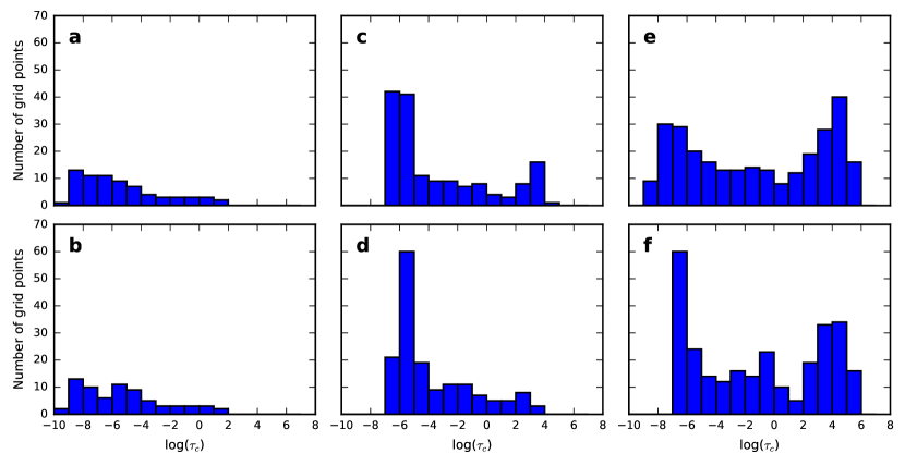
Figure 4.— Histograms of grid-point density for the different atmospheric models considered here: a) FALC, b) FALF, c) Bifrost-1, d) Bifrost-2, e) CO⁵BOLD-1, and f) CO⁵BOLD-2.

The formal solvers presented in Section 3 are tested on the atmospheric models shown in Figure 3 with the spectral lines given in Table 1. The atmospheric models are re-sampled homogeneously in $\log\tau_{c}$ with different grid-point densities (see Section 4): the FAL atmospheric models are re-sampled in the optical depth interval $-8.6\leq\log\tau_{c}\leq 1.4$, the Bifrost vertical columns in $-6.5\leq\log\tau_{c}\leq 3.5$, and the CO⁵BOLD vertical columns in $-8\leq\log\tau_{c}\leq 2$. Each spectral line is sampled with around 500 points equispaced in frequency in a spectral interval of a few Å around the core. The global error is defined by Equation (B1).

Figure 5 shows the emerging Stokes profiles, synthesized with the second-order pragmatic method for three different poorly-sampled atmospheric models. Figures 7-11 give the log-log representation of the global error in the emergent Stokes vector profiles as a function of the number of ppd of continuum optical depth. It would certainly be incautious to draw drastic conclusions on the basis of a qualitative comparison of small details of the error curves. However, the numerical tests allow for different general considerations. The numerical results are listed in the following according the formation regions of the spectral lines. Note that there is a limit (usually for $\geq 50$ ppd) beyond which the accuracy of fourth-order methods is limited by machine precision and the fourth-order convergence may not be respected anymore.

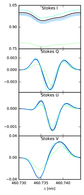
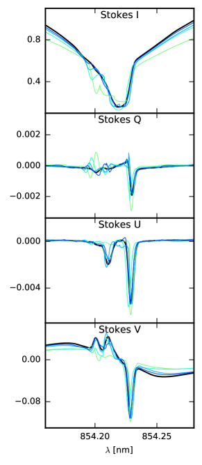
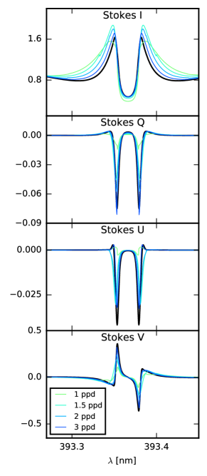
Figure 5.— Emerging Stokes profiles calculated with the second-order pragmatic method for the Sr i line at 4607.3 Å for the Bifrost-1 atmospheric model (first column); the Ca ii line at 8542.1 Å for the CO⁵BOLD-2 atmospheric model (second column); and the Ca ii line at 3933.7 Å for the FALC atmospheric model (third column). The atmospheric models are described in Figure 3. The different colors indicate different grid-point densities according the coding in the inset at the bottom of the last column. The reference emergent Stokes profile (solid black) is calculated using a sampling with $10^{3}$ ppd.

5.1. Photospheric spectral lines

This section analyzes the numerical synthesis of the photospheric Sr i line at 4607.3 Å and Fe i lines at 6301.5 and 6302.5 Å. Bianda, M. et al. (2018) use the Sr i 4607.3 Å spectral line to infer the spatial and temporal variation of the weak subgranular magnetic field with the Hanle effect. Moreover, Alsina Ballester et al. (2017) studied this spectral line considering PRD phenomena in the general Hanle-Zeeman regime. The Fe i spectral lines at 6301.5 and 6302.5 Å are often used to determine the magnetic field vector in the solar photosphere, and they are the standard lines of the Advanced Spectropolarimeter (Skumanich et al., 1994) and of the Hinode Spectropolarimeter (Tsuneta et al., 2008). Moreover, Bellot Rubio et al. (1998) and, lately, de la Cruz Rodríguez & Piskunov (2013) already used these spectral lines to analyze the performances of different formal solvers.

Here, these photospheric lines are synthesized under the assumption of LTE conditions. The comparison of the first and second row of Figure 7 does not reveal any essential difference between the error curves of the FAL and the Bifrost atmospheric models. In fact, the behavior of these discrete models do not differ very much in the photosphere, while Figure 7 indicates that the higher intermittency of the CO⁵BOLD-1 model weakens the performance of high-order methods.

It is very difficult to judge and compare the different formal solvers in the pre-asymptotic regime (i.e., where the convergence rate of numerical schemes may be not respected). Indeed, insufficient grid-point densities do not allow for high-order convergence and the accuracy of numerical schemes strongly depends on the specific sampling. In any case, errors in the pre-asymptotic regime are usually $\geq 10^{-1}$ and the synthesized Stokes profiles cannot be considered accurate. The first column of Figure 5 gives a glimpse on the stable pre-asymptotic behavior of the second-order pragmatic method in the synthesis of the Sr i line at 4607.3 Å with very coarse Bifrost-1 grids.

Asymptotic convergence rates become relevant above 3 ppd. In this regime, high-order schemes outperform low-order methods: fourth-order methods require among 10-15 ppd to achieve an accuracy of $E_{i}\leq 10^{-4}$, for $i=1,2,3,4$ (see Equation (B1)). Third-order methods need about twice as many ppd to reach the same accuracy, whereas second-order methods require prohibitive numerical grids to produce such highly accurate spectra.

In the asymptotic regime, the accuracy and the order of convergence achieved by DELO methods and corresponding order non-DELO methods (with the exception of the pragmatic formal solvers) are almost identical and no clear differences are visible. Second- and third-order pragmatic methods achieve the predicted order of accuracy.

5.2. Lower chromospheric spectral lines

This section analyzes the numerical synthesis of the Ba ii line at 4554.0 Å and the central line of the Ca ii infrared triplet at 8542.1 Å. The high photospheric/low chromospheric Ba ii 4554.0 Å line drew attention because of the magnetic sensitivity of the strong scattering polarization signal that it shows in the so-called Second Solar Spectrum (e.g., Stenflo, 1997; Belluzzi et al., 2007; Faurobert et al., 2009; Ramelli et al., 2009; Smitha et al., 2013). The low chromospheric Ca ii 8542.1 Å line has been extensively used as diagnostics because of its high sensitivity to photospheric and chromospheric responses (de la Cruz Rodríguez & Piskunov, 2013; Quintero Noda et al., 2016).

Here, NLTE effects are included for both spectral lines in terms of the field-free approximation. The comparison of the first and second row of Figures 9 and 9 shows relevant differences between the error curves of FAL and R-MHD atmospheric models. The intermittency of R-MHD single-pixel models in the low chromosphere weakens the performance of high-order methods. In fact, the break-even point where high-order methods start to outperform low-order methods depends on the smoothness of the atmospheric model: it is at about 5 ppd when using FAL models and at 10-15 ppd for the Bifrost-2 model. The strongly intermittent behavior in the outer layers of the CO⁵BOLD atmospheric models thwarts high-order convergence below 20-30 ppd, defeating the purpose of using high-order methods. For a given accuracy, the synthesis of chromospheric spectral lines generally requires a slightly higher density of grid points than the synthesis of photospheric spectral lines. This is also due to the chosen homogeneous sampling in $\log\tau_{c}$, which is more suitable for the synthesis of spectral lines forming around $\tau_{c}=1$ than to spectral lines forming in higher layers of the atmosphere.

The DELO-linear method usually maintains the pre-asymptotic error smaller than the trapezoidal method. This is due to the accurate representation of the fast exponential attenuation of optically thick cells guaranteed by its $L$-stability. The occurrence of numerical instability of high-order methods is evident: the Adams-Moulton 3 method shows strong instabilities when treating optically thick cells, because of its limited stability region. Moreover, the global error of both Adams-Moulton 3 and DELO-parabolic methods grows, instead of decreasing, as the density of grid points increases. Additional numerical test calculations have excluded that round-off errors are the cause of this kind of instability, which instead might be due to the compound effect of variable cell size and variable propagation matrix coefficients, that modifies the stability function of multistep methods. The second column of Figure 5 shows the synthesis of the Ca ii 8542.1 Å performed by the second-order pragmatic method with very coarse CO⁵BOLD-2 grids. It demonstrates that this method is stable even in the case of intermittent poorly-sampled atmospheric models.

The accuracy and the order of convergence achieved by DELO methods and corresponding order non-DELO methods are almost identical in the asymptotic regime. Similarly to the case of photospheric lines, the second- and third-order pragmatic methods do not suffer from numerical instability and achieve the predicted order of accuracy. In some cases, they even achieve higher accuracy with respect to corresponding order schemes.

5.3. Upper chromospheric spectral lines

This section analyzes the numerical synthesis of the Ca ii K line at 3933.7 Å and the Mg ii k line at 2795.5 Å. The Ca ii K line is the strongest spectral line in the visible solar spectrum, shows very extended wings, and forms across a large range of atmospheric heights. The core region is of particular interest because it carries information on the physical conditions of the high chromosphere (e.g., Solanki et al., 1991; Carlsson & Stein, 1997; Solanki, 2004; Anusha & Nagendra, 2013; Bjørgen et al., 2018). The Mg ii k line is an important diagnostics of the Interface Region Imaging Spectrograph (IRIS) space telescope (De Pontieu et al., 2014). Moreover, Leenaarts et al. (2013a, b) synthesized the intensity profile of this spectral line from 3D R-MHD solar atmospheric models considering PRD. Scattering polarization in this line has been modeled with a FALC atmosphere accounting for PRD effects by Belluzzi & Trujillo Bueno (2012) and, subsequently, Alsina Ballester et al. (2016) also took the joint action of the Hanle and Zeeman effects into account. The new instrument “Chromospheric LAyer SpectroPolarimeter” drew additional interest toward this spectral line (CLASP2, Narukage et al., 2016).

Here, NLTE effects are included for both spectral lines in terms of the field-free approximation. Figures 11 and 11 show that high-order methods are well-performing for the case of the smooth FAL atmospheric models only. Numerical methods perform very inefficiently in the absence of sufficient local smoothness because discontinuities (or sharp gradients) might drastically increase local errors, thwarting high-order convergence (e.g., Dieci & Lopez, 2012). In practice, the high intermittency of the Bifrost and CO⁵BOLD single-column models in the chromospheric layers leads to an order of convergence “breakdown”, making the application of high-order schemes pointless (e.g., Mannshardt, 1978).

The CO⁵BOLD-2 atmosphere used for the convergence plots of Figure 11 (bottom row) has no proper chromospheric temperature rise. Correspondingly, the core of the Mg ii k line has no k₂ emission peaks in this case. This may not seem realistic bearing non-resolved observed profiles with clear k₂v and k₂r emission peaks and a central k₃ core in mind. However, single columns of 3D R-MHD models show a large variety of temperature profiles, and Leenaarts et al. (2013b) report that 0.1% of the Mg ii h and k profiles from a Bifrost model atmosphere did not have any emission peaks, although normally the Bifrost model features a proper chromospheric temperature rise and transition zone. For this reason, this seemingly unrealistic example is included in the numerical tests.

Once again, the DELO-linear method usually maintains the pre-asymptotic error equal or smaller than the corresponding error of the trapezoidal method. Adams-Moulton 3 and DELO-parabolic methods suffer from the same instability issues already encountered with the synthesis of low chromospheric lines. The third column of Figure 5 gives a glimpse on the pre-asymptotic stable behavior of the second-order pragmatic method in the synthesis of the Ca ii K line with very coarse FALC grids.

As for the previous cases, the accuracy and the order of convergence achieved by DELO methods and corresponding order non-DELO methods are almost identical in the asymptotic regime. As before, second- and third-order pragmatic methods do not suffer from numerical instability, achieving the predicted order of accuracy.

Note that the homogeneous sampling in $\log\tau_{c}$ might not be suitable for analyzing the synthesis of Stokes profiles of upper chromospheric spectral lines, whose cores are forming far away from the formation region of the continuum. However, alternative tests on atmospheric models re-sampled homogeneously in $\log\tau_{\ell}$ (where $\tau_{\ell}$ indicates the line center optical depth) show similar results.

6. Conclusions

This paper investigates different actors that play a relevant role in the numerical integration of the polarized radiative transfer equation: in particular, the numerical scheme, the atmospheric model (and its sampling), and the spectral line. Special attention is paid to assess the mathematical predictions given by Janett et al. (2017b, a) and Janett & Paganini (2018), who characterized different formal solvers (in terms of order of accuracy, numerical stability, and computational cost) and investigated the stiffness of Equation (1). Although NLTE effects are taken into account in the computation of the considered spectral lines, the analysis is limited to the numerical integration of Equation (1) and does not concern the full NLTE iterative problem.

The urgency of high-order formal solvers has been often promoted, e.g., in LTE inversions (Bellot Rubio et al., 1998) and in full NLTE problems (Trujillo Bueno, 2003). On the other hand, the numerical tests in Section 5 indicate that the use of high-order methods is befitting only if the relevant layers of the atmospheric model guarantee sufficient smoothness in the solution (i.e., when the pre-asymptotic behavior of the error curve is avoided). In the case of FAL models, high-order schemes generally outperform low-order methods with a density of grid points larger than 3-5 ppd. Meanwhile, the high intermittency of 3D R-MHD models might thwart high-order convergence even in fine numerical grids, making the application of high-order schemes pointless (or even noxious). In the asymptotic regime, the accuracy achieved by DELO methods and corresponding order non-DELO methods is almost identical.

The numerical results confirm the predictions given by Janett & Paganini (2018). First, Figure 2 shows that the conversion to optical depth effectively removes stiffness from Equation (1) because it attenuates variation of the propagation matrix elements along the integration path. Second, $L$-stability guarantees the exponential attenuations of the radiation across optically thick cells, avoiding numerical oscillations. Consequently, the $L$-stable DELO-linear method always keeps the error $E_{i}\leq 1$ (for $i=1,2,3,4$) and it is, consequently, particularly suitable to coarse atmospheric models with optically thick cells. Third, the Adams-Moulton 3 method shows strong instabilities when treating optically thick cells because of its limited stability region. In addition, both Adams-Moulton 3 and DELO-parabolic methods occasionally present a particular kind of numerical instability, where the global error grows as the density of grid points increases. The origin of this kind of instability might be the compound effect of variable cell size and variable propagation matrix coefficients, which modify the stability function of multistep methods. For this reason, multistep schemes are not recommended for practical applications. Furthermore, the Bézier strategy (intended to avoid overshooting in the absorption and emission coefficients) does not provide better results when treating realistic and intermittent atmospheric models. This is shown by the second row of Figures 7-11, which expose the congruence between cubic Bézier method and the cubic Hermitian method.

The choice of the optimal formal solver definitely depends on the particular problem, when opting for the cheapest numerical scheme that satisfies accuracy requirements (and ensures numerical stability). In conclusion, if the atmospheric model lacks sufficient local smoothness or if a relatively large error is accepted (say $E_{i}\approx 10^{-2}$), the second-order pragmatic method is recommended and the DELO-linear method still represents a solid alternative with an easier implementation. If higher accuracy is necessary (say $E_{i}\leq 10^{-3}$) and smoothness in atmospheric models is guaranteed, the third-order pragmatic method is recommended.

The performance of the numerical methods on discontinuous atmospheric models requires a deeper investigation. However, the structure of pragmatic methods might also be suitable to switch to suitable techniques, when facing discontinuities in the integration interval.

Appendix A Pragmatic methods pseudocodes

for $i=1$ to $N$ do

       compute $\Delta\tau$, $\phi_{\text{\rm\tiny H}}$, and $\phi_{\text{\rm\tiny T}}$;

       if $(\phi_{\text{\rm\tiny H}}<1\;\lor\;\Delta\tau<\tau_{1})$ then

            

            $\Rightarrow$ Heun’s method ($\mathbf{\Psi}^{E}$);

            

       else if $(\phi_{\text{\rm\tiny T}}<1\;\land\;\Delta\tau<\tau_{2})$ then

            

            $\Rightarrow$ Trapezoidal method ($\mathbf{\Psi}^{A}$);

            

      else

            $\Rightarrow$ DELO-linear method ($\mathbf{\Psi}^{L}$);

            

       end if

      

end for

Algorithm 1 Second-order pragmatic method. The choice of free parameters $\tau_{1}=10^{-3}$ and $\tau_{2}=7$ has proven good results.

for $i=1$ to $N$ do

       compute $\Delta\tau$, $\phi_{\text{\rm\tiny RK3}}$, and $\phi_{\text{\rm\tiny H3}}$;

       if $(\phi_{\text{\rm\tiny RK3}}<1\;\lor\;\Delta\tau<\tau_{1})$ then

            

            $\Rightarrow$ Runge-Kutta 3 method ($\mathbf{\Psi}^{E}$);

            

       else if $(\phi_{\text{\rm\tiny H3}}<1\;\land\;\Delta\tau<\tau_{2})$ then

            

            $\Rightarrow$ Hermitian 3 method ($\mathbf{\Psi}^{A}$);

            

      else

            $\Rightarrow$ DELO-linear method ($\mathbf{\Psi}^{L}$);

            

       end if

      

end for

Algorithm 2 Third-order pragmatic method. The choice of free parameters $\tau_{1}=10^{-3}$ and $\tau_{2}=10$ has proven good results.

Appendix B Error calculation

Denoting with $\mathbf{I}^{\rm ref}(\nu)$ and $\mathbf{I}^{\rm num}(\nu)$ the reference and the numerically computed emergent Stokes vectors, respectively, at the frequency $\nu$, the global error for each Stokes vector component is computed as

$$E_{i}=\frac{\displaystyle\max_{\nu}|I_{i}^{\rm ref}(\nu)-I_{i}^{\rm num}(\nu)|}{{\displaystyle\max_{\nu}}\;I_{i}^{\rm ref}(\nu)-{\displaystyle\min_{\nu}}\;I_{i}^{\rm ref}(\nu)}\,,\text{ for }i=1,2,3,4\,,$$ (B1)

where $i=1,2,3,4$ indicate the four Stokes parameters $(I,Q,U,V)$. The error is given by the maximal discrepancy between the reference and the simulated Stokes parameter over the spectral interval considered, normalized by the maximal amplitude in the reference profile. The reference emergent Stokes profile is calculated with the cubic Hermitian method (and cross-checked with the quadratic DELO-Bézier method) using a hyperfine grid sampling with $10^{3}$ ppd of continuum optical depth. The infinite norm used for the global error is sensitive to outliers at single wavelengths and error curves may show non-monotonic behavior, especially in pre-asymptotic regime.

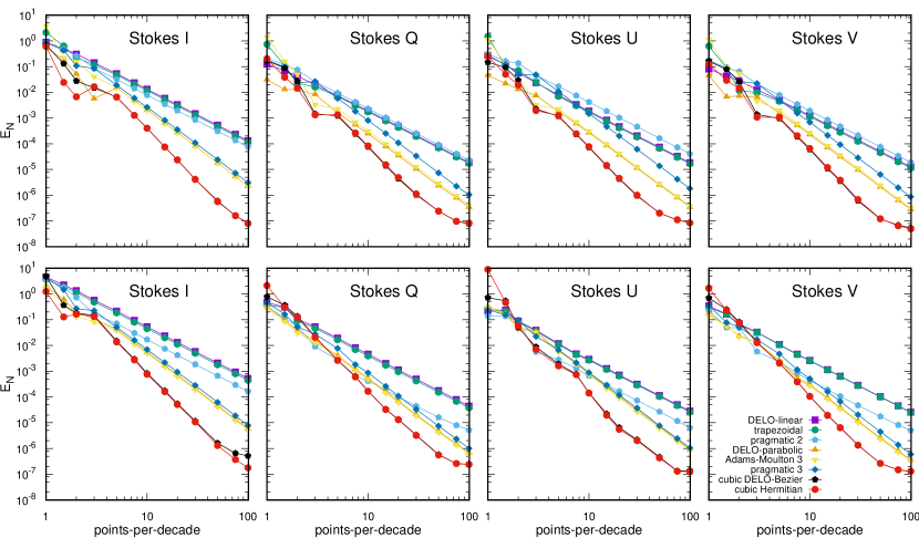
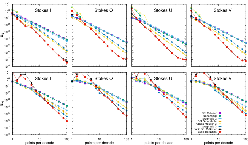
Figure 6.— The log-log representation of the global error for the Stokes vector components $I,Q,U$, and $V$ as a function of the number of ppd of continuum optical depth for the formal solvers (color-coded) presented in Section 3. The Sr i line at 4607.3 Å is considered for the FALC atmospheric model (first row) and the Bifrost-1 atmospheric model (second row). The atmospheric models are described in Figure 3. The global error is computed as exposed in Appendix B.

Figure 7.— Same as Figure 7, but for the Fe i lines at 6301.5 and 6302.5 Å, respectively, and for the FALF atmospheric model (first row) and the CO⁵BOLD-1 atmospheric model (second row).

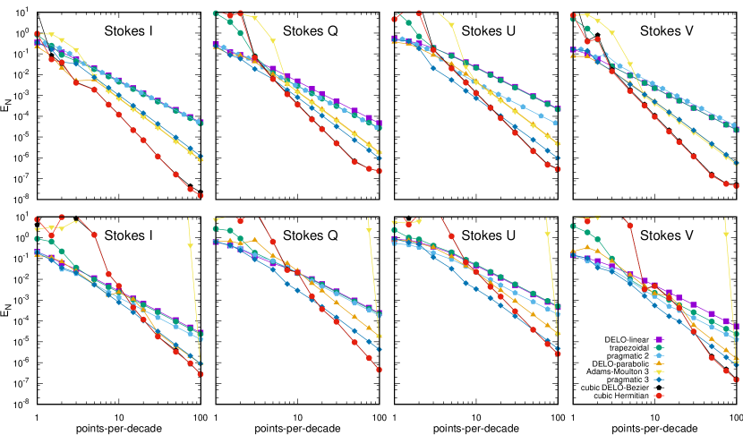
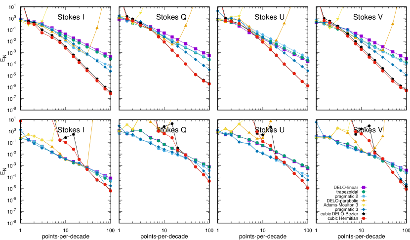
Figure 8.— Same as Figure 7, but for the Ba ii line at 4554.0 Å and for the FALC atmospheric model (first row) and the Bifrost-2 atmospheric model (second row).

Figure 9.— Same as Figure 7, but for the infrared Ca ii line at 8542.1 Å and for the FALF atmospheric model (first row) and the CO⁵BOLD-2 atmospheric model (second row).

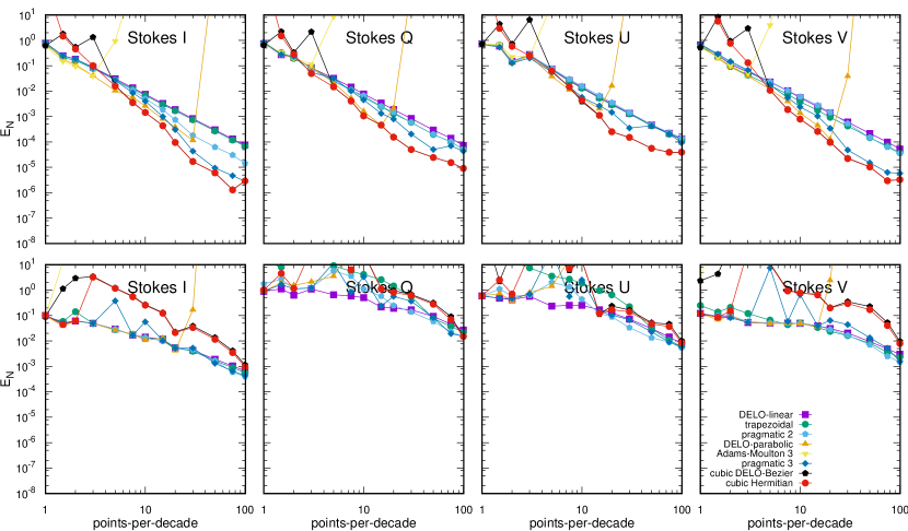
Figure 10.— Same as Figure 7, but for the Ca ii K line at 3933.7 Å and for the FALC atmospheric model (first row) and the Bifrost-2 atmospheric model (second row).

Figure 11.— Same as Figure 7, but for the Mg ii k line at 2795.5 Å and for the FALF atmospheric model (first row) and the CO⁵BOLD-2 atmospheric model (second row).

References

- Alsina Ballester et al. (2016) Alsina Ballester, E., Belluzzi, L., & Trujillo Bueno, J. 2016, ApJ, 831, L15
- Alsina Ballester et al. (2017) —. 2017, ApJ, 836, 6
- Anusha & Nagendra (2013) Anusha, L. S., & Nagendra, K. N. 2013, ApJ, 767, 108
- Auer (2003) Auer, L. 2003, in Astronomical Society of the Pacific Conference Series, Vol. 288, Stellar Atmosphere Modeling, ed. I. Hubeny, D. Mihalas, & K. Werner, 3
- Bellot Rubio et al. (1998) Bellot Rubio, L. R., Ruiz Cobo, B., & Collados, M. 1998, ApJ, 506, 805
- Bellot Rubio et al. (2000) —. 2000, ApJ, 535, 475
- Belluzzi & Trujillo Bueno (2012) Belluzzi, L., & Trujillo Bueno, J. 2012, ApJ, 750, L11
- Belluzzi et al. (2007) Belluzzi, L., Trujillo Bueno, J., & Landi Degl’Innocenti, E. 2007, ApJ, 666, 588
- Bianda, M. et al. (2018) Bianda, M., Berdyugina, S., Gisler, D., Ramelli, R., Belluzzi, L., Carlin, E. S., Stenflo, J. O., & Berkefeld, T. 2018, A&A, 614, A89
- Bjørgen et al. (2018) Bjørgen, J. P., Sukhorukov, A. V., Leenaarts, J., Carlsson, M., de la Cruz Rodríguez, J., Scharmer, G. B., & Hansteen, V. H. 2018, A&A, 611, A62
- Calvo et al. (2016) Calvo, F., Steiner, O., & Freytag, B. 2016, A&A, 596, A43
- Carlin & Bianda (2017) Carlin, E. S., & Bianda, M. 2017, ApJ, 843, 64
- Carlsson et al. (2016) Carlsson, M., Hansteen, V. H., Gudiksen, B. V., Leenaarts, J., & De Pontieu, B. 2016, A&A, 585, A4
- Carlsson & Stein (1997) Carlsson, M., & Stein, R. F. 1997, ApJ, 481, 500
- de la Cruz Rodríguez & Piskunov (2013) de la Cruz Rodríguez, J., & Piskunov, N. 2013, ApJ, 764, 33
- de la Cruz Rodríguez & van Noort (2017) de la Cruz Rodríguez, J., & van Noort, M. 2017, Space Sci. Rev., 210, 109
- De Pontieu et al. (2014) De Pontieu, B., Title, A. M., Lemen, J. R., Kushner, G. D., Akin, D. J., Allard, B., Berger, T., Boerner, P., Cheung, M., Chou, C., Drake, J. F., Duncan, D. W., Freeland, S., Heyman, G. F., Hoffman, C., Hurlburt, N. E., Lindgren, R. W., Mathur, D., Rehse, R., Sabolish, D., Seguin, R., Schrijver, C. J., Tarbell, T. D., Wülser, J.-P., Wolfson, C. J., Yanari, C., Mudge, J., Nguyen-Phuc, N., Timmons, R., van Bezooijen, R., Weingrod, I., Brookner, R., Butcher, G., Dougherty, B., Eder, J., Knagenhjelm, V., Larsen, S., Mansir, D., Phan, L., Boyle, P., Cheimets, P. N., DeLuca, E. E., Golub, L., Gates, R., Hertz, E., McKillop, S., Park, S., Perry, T., Podgorski, W. A., Reeves, K., Saar, S., Testa, P., Tian, H., Weber, M., Dunn, C., Eccles, S., Jaeggli, S. A., Kankelborg, C. C., Mashburn, K., Pust, N., Springer, L., Carvalho, R., Kleint, L., Marmie, J., Mazmanian, E., Pereira, T. M. D., Sawyer, S., Strong, J., Worden, S. P., Carlsson, M., Hansteen, V. H., Leenaarts, J., Wiesmann, M., Aloise, J., Chu, K.-C., Bush, R. I., Scherrer, P. H., Brekke, P., Martinez-Sykora, J., Lites, B. W., McIntosh, S. W., Uitenbroek, H., Okamoto, T. J., Gummin, M. A., Auker, G., Jerram, P., Pool, P., & Waltham, N. 2014, Sol. Phys., 289, 2733
- del Toro Iniesta & Ruiz Cobo (2016) del Toro Iniesta, J. C., & Ruiz Cobo, B. 2016, Living Reviews in Solar Physics, 13, 4
- Dieci & Lopez (2012) Dieci, L., & Lopez, L. 2012, Journal of Computational and Applied Mathematics, 236, 3967
- Faurobert et al. (2009) Faurobert, M., Derouich, M., Bommier, V., & Arnaud, J. 2009, A&A, 493, 201
- Fontenla et al. (1990) Fontenla, J. M., Avrett, E. H., & Loeser, R. 1990, ApJ, 355, 700
- Fontenla et al. (1991) —. 1991, ApJ, 377, 712
- Fontenla et al. (1993) —. 1993, ApJ, 406, 319
- Fontenla et al. (1999) Fontenla, J. M., White, O. R., Fox, P. A., Avrett, E. H., & Kurucz, R. L. 1999, ApJ, 518, 480
- Frank & Leimkuhler (2012) Frank, J., & Leimkuhler, B. 2012, Computational Modelling and Dynamical Systems, Lecture Notes (Universities of Amsterdam and Edinburgh)
- Freytag et al. (2012) Freytag, B., Steffen, M., Ludwig, H.-G., Wedemeyer-Böhm, S., Schaffenberger, W., & Steiner, O. 2012, Journal of Computational Physics, 231, 919
- Fritsch & Butland (1984) Fritsch, F. N., & Butland, J. 1984, SIAM Journal on Scientific and Statistical Computing, 5, 300
- Geart & Tu (1974) Geart, C. W., & Tu, K. W. 1974, SIAM Journal on Numerical Analysis, 11, 1025
- Gingerich et al. (1971) Gingerich, O., Noyes, R. W., Kalkofen, W., & Cuny, Y. 1971, Sol. Phys., 18, 347
- Grigorieff (1983) Grigorieff, R. D. 1983, Numerische Mathematik, 42, 359
- Grossmann-Doerth et al. (1988) Grossmann-Doerth, U., Schüssler, M., & Solanki, S. K. 1988, A&A, 206, L37
- Gudiksen et al. (2011) Gudiksen, B. V., Carlsson, M., Hansteen, V. H., Hayek, W., Leenaarts, J., & Martínez-Sykora, J. 2011, A&A, 531, A154
- Hairer et al. (2000) Hairer, E., Nørsett, S., & Wanner, G. 2000, Solving Ordinary Differential Equations I Nonstiff problems, 2nd edn. (Berlin: Springer)
- Holweger & Mueller (1974) Holweger, H., & Mueller, E. A. 1974, Sol. Phys., 39, 19
- Ibgui et al. (2013) Ibgui, L., Hubeny, I., Lanz, T., & Stehlé, C. 2013, A&A, 549, A126
- Janett et al. (2017a) Janett, G., Carlin, E. S., Steiner, O., & Belluzzi, L. 2017a, ApJ, 840, 107
- Janett & Paganini (2018) Janett, G., & Paganini, A. 2018, ApJ, 857, 91
- Janett et al. (2017b) Janett, G., Steiner, O., & Belluzzi, L. 2017b, ApJ, 845, 104
- Kunasz & Auer (1988) Kunasz, P., & Auer, L. H. 1988, J. Quant. Spec. Radiat. Transf., 39, 67
- Landi Degl’Innocenti (1987) Landi Degl’Innocenti, E. 1987, in Numerical Radiative Transfer, ed. W. Kalkofen (Cambridge University Press), 265–278
- Landi Degl’Innocenti & Landolfi (2004) Landi Degl’Innocenti, E., & Landolfi, M. 2004, Astrophysics and Space Science Library, Vol. 307, Polarization in Spectral Lines (Dordrecht: Kluwer Academic Publishers)
- Leenaarts et al. (2013a) Leenaarts, J., Pereira, T. M. D., Carlsson, M., Uitenbroek, H., & De Pontieu, B. 2013a, ApJ, 772, 89
- Leenaarts et al. (2013b) —. 2013b, ApJ, 772, 90
- López Ariste & Semel (1999) López Ariste, A., & Semel, M. 1999, A&A, 350, 1089
- Magain (1986) Magain, P. 1986, A&A, 163, 135
- Mannshardt (1978) Mannshardt, R. 1978, Numerische Mathematik, 31, 131
- Mauas (2007) Mauas, P. 2007, in Astronomical Society of the Pacific Conference Series, Vol. 368, The Physics of Chromospheric Plasmas, ed. P. Heinzel, I. Dorotovič, & R. J. Rutten, Heinzel
- Mihalas et al. (1978) Mihalas, D., Auer, L. H., & Mihalas, B. R. 1978, ApJ, 220, 1001
- Murphy (1990) Murphy, G. A. 1990, PhD thesis, Univ. Sidney, (1990)
- Narukage et al. (2016) Narukage, N., McKenzie, D. E., Ishikawa, R., Trujillo-Bueno, J., De Pontieu, B., Kubo, M., Ishikawa, S.-n., Kano, R., Suematsu, Y., Yoshida, M., Rachmeler, L. A., Kobayashi, K., Cirtain, J. W., Winebarger, A. R., Asensio Ramos, A., del Pino Aleman, T., Štȩpán, J., Belluzzi, L., Larruquert, J. I., Auchère, F., Leenaarts, J., & Carlsson, M. J. L. 2016, in , 990508
- Pereira & Uitenbroek (2015) Pereira, T. M. D., & Uitenbroek, H. 2015, A&A, 574, A3
- Piskunov & Kochukhov (2002) Piskunov, N., & Kochukhov, O. 2002, A&A, 381, 736
- Quintero Noda et al. (2016) Quintero Noda, C., Shimizu, T., de la Cruz Rodríguez, J., Katsukawa, Y., Ichimoto, K., Anan, T., & Suematsu, Y. 2016, MNRAS, 459, 3363
- Rachkovsky (1967) Rachkovsky, D. N. 1967, Izvestiya Ordena Trudovogo Krasnogo Znameni Krymskoj Astrofizicheskoj Observatorii, 37, 56
- Ramelli et al. (2009) Ramelli, R., Bianda, M., Trujillo Bueno, J., Belluzzi, L., & Landi Degl’Innocenti, E. 2009, in Astronomical Society of the Pacific Conference Series, Vol. 405, Solar Polarization 5: In Honor of Jan Stenflo, ed. S. V. Berdyugina, K. N. Nagendra, & R. Ramelli, 41
- Rees (1969) Rees, D. E. 1969, Solar Physics, 10, 268
- Rees et al. (1989) Rees, D. E., Durrant, C. J., & Murphy, G. A. 1989, ApJ, 339, 1093
- Ruiz Cobo & del Toro Iniesta (1992) Ruiz Cobo, B., & del Toro Iniesta, J. C. 1992, ApJ, 398, 375
- Rybicki & Hummer (1991) Rybicki, G. B., & Hummer, D. G. 1991, A&A, 245, 171
- Rybicki & Hummer (1992) —. 1992, A&A, 262, 209
- Rybicki & Hummer (1994) —. 1994, A&A, 290, 553
- Skumanich et al. (1994) Skumanich, A., Lites, B. W., & Pillet, V. M. 1994, in Solar Surface Magnetism, ed. R. J. Rutten & C. J. Schrijver, NATO Advanced Science Institutes (ASI) Series C (Dordrecht: Springer Netherlands), 99–125
- Smitha et al. (2013) Smitha, H. N., Nagendra, K. N., Stenflo, J. O., & Sampoorna, M. 2013, ApJ, 768, 163
- Solanki (2004) Solanki, S. K. 2004, in IAU Symposium, Vol. 223, Multi-Wavelength Investigations of Solar Activity, ed. A. V. Stepanov, E. E. Benevolenskaya, & A. G. Kosovichev, 195–202
- Solanki et al. (1991) Solanki, S. K., Steiner, O., & Uitenbroek, H. 1991, A&A, 250, 220
- Steffen (1990) Steffen, M. 1990, A&A, 239, 443
- Steiner et al. (2017) Steiner, O., Calvo, F., Salhab, R., & Vigeesh, G. 2017, Mem. Soc. Astron. Italiana, 88, 37
- Stenflo (1994) Stenflo, J. O. 1994, Solar Magnetic Fields (Dordrecht: Kluwer Academic Publishers)
- Stenflo (1997) Stenflo, J. O. 1997, A&A, 324, 344
- Stenholm & Stenflo (1977) Stenholm, L. G., & Stenflo, J. O. 1977, A&A, 58, 273
- Trujillo Bueno (2003) Trujillo Bueno, J. 2003, in Astronomical Society of the Pacific Conference Series, Vol. 288, Stellar Atmosphere Modeling, ed. I. Hubeny, D. Mihalas, & K. Werner, 551
- Tsuneta et al. (2008) Tsuneta, S., Ichimoto, K., Katsukawa, Y., Nagata, S., Otsubo, M., Shimizu, T., Suematsu, Y., Nakagiri, M., Noguchi, M., Tarbell, T., Title, A., Shine, R., Rosenberg, W., Hoffmann, C., Jurcevich, B., Kushner, G., Levay, M., Lites, B., Elmore, D., Matsushita, T., Kawaguchi, N., Saito, H., Mikami, I., Hill, L. D., & Owens, J. K. 2008, Sol. Phys., 249, 167
- Uitenbroek (2001) Uitenbroek, H. 2001, ApJ, 557, 389
- Unno (1956) Unno, W. 1956, PASJ, 8, 108
- Štěpán & Trujillo Bueno (2013) Štěpán, J., & Trujillo Bueno, J. 2013, A&A, 557, A143
- Štěpán et al. (2015) Štěpán, J., Trujillo Bueno, J., Leenaarts, J., & Carlsson, M. 2015, ApJ, 803, 65
- Vernazza et al. (1981) Vernazza, J. E., Avrett, E. H., & Loeser, R. 1981, ApJS, 45, 635