Node Classification for Signed Social Networks Using Diffuse Interface Methods

Abstract

Signed networks contain both positive and negative kinds of interactions like friendship and enmity. The task of node classification in non-signed graphs has proven to be beneficial in many real world applications, yet extensions to signed networks remain largely unexplored. In this paper we introduce the first analysis of node classification in signed social networks via diffuse interface methods based on the Ginzburg-Landau functional together with different extensions of the graph Laplacian to signed networks. We show that blending the information from both positive and negative interactions leads to performance improvement in real signed social networks, consistently outperforming the current state of the art.

1 Introduction

Signed graphs are graphs with both positive and negative edges, where positive edges encode relationships like friendship and trust, and negative edges encode conflictive and enmity interactions. Recently, signed graphs have received an increasing amount of attention due to its capability to encode interactions that are not covered by unsigned graphs or multilayer graphs [41, 48, 52, 59, 54], which mainly encode interactions based on similarity and trust. While the analysis of unsigned graphs follows a long-standing and well established tradition [40, 45, 5], the analysis of signed graphs can be traced back to [10, 30], in the context of social balance theory, further generalized in [17] by introducing the concept of a $k$-balance signed graph: a signed graph is $k$-balanced if the set of nodes can be partitioned into $k$ disjoint sets such that inside the sets there are only positive relationships, and between different sets only negative relationships. A related concept is constrained clustering [2], where must-links and cannot-links are constraints indicating if certain pairs of nodes should be assigned to the same or different clusters. Recent developments of signed graphs have been guided by the concept of $k$-balance, leading to a diverse paradigm of applications, including: clustering [20, 13, 35, 42, 47, 32, 15, 16, 43], edge prediction [34, 36, 23], node embeddings [18, 31, 55, 57], node ranking [14, 49], node classification [50], and many more. See [51, 24] for a recent survey on the topic. One task that remains largely unexplored is the task of node classification in signed networks. The problem of node classification in graphs is a semi-supervised learning problem where the goal is to improve classification performance by taking into account both labeled and unlabeled observations [61, 11], being a particular case graph-based semi-supervised learning. The task of graph-based classification methods on unsigned graphs is a fundamental problem with many application areas [58, 60, 3]. A technique that has recently been proposed with very promising results utilizes techniques known from partial differential equations in materials science and combines these with graph based quantities (cf. [5]). In particular, the authors in [5] use diffuse interface methods that are derived from the Ginzburg–Landau energy [1, 6, 27, 53]. These methods have been used in image inpainting where a damaged region of an image has to be restored given information about the undamaged image parts. In the context of node classification in graphs, the undamaged part of an image corresponds to labeled nodes, whereas the damaged part corresponds to unlabeled nodes to be classified based on the information of the underlying graph structure of the image and available labeled nodes. With this analogy, one can readily use results from [4] for the classification problem on graphs. While the materials science problems are typically posed in an infinite-dimensional setup, the corresponding problem in the graph-based classification problem uses the graph Laplacian. This technique has shown great potential and has recently been extended to different setups [7, 25, 44]. Our contributions are as follows: we study the problem of node classification in signed graphs by developing a natural extension of diffuse interface schemes of Bertozzi and Flenner [5], based on different signed graph Laplacians. To the best of our knowledge this is the first study of node classification in signed networks using diffuse interface schemes. A main challenge when considering the application of diffuse interface methods to signed networks is the availability of several competing signed graph Laplacians and how the method’s performance depends on the chosen signed graph Laplacian, hence we present a thorough comparison of our extension based on existing signed graph Laplacians. Further, we show the effectivity of our approach against state of the art approaches by performing extensive experiments on real world signed social networks. The paper is structured as follows. We first introduce the tools needed from graphs and how they are extended to signed networks. We study the properties of several different signed Laplacians. We then introduce a diffuse interface technique in their classical setup and illustrate how signed Laplacians can be used within the diffuse interface approach. This is then followed by numerical experiments in real world signed networks.

Reproducibility: Our code is available at https://github.com/melopeo/GL

2 Graph information and signed networks

We now introduce the Laplacian for unsigned graphs followed by particular versions used for signed graphs.

2.1 Laplacians for unsigned graphs

In this section we introduce several graph Laplacians, which are the main tools for our work. Let $G=(V,W)$ be an undirected graph with node set $V=\{v_{1},\ldots,v_{n}\}$ of size $n=\left|V\right|$ and adjacency matrix $W\in\mathbb{R}^{n\times n}$ with non-negative weights, i.e., $w_{ij}\geq 0$. In the case where a graph presents an assortative configuration, i.e. edge weights of the adjacency matrix $W$ represent similarities (the larger the value of $w_{ij}$ the larger the similarity of nodes the $v_{i}$ and $v_{j}$), then the Laplacian matrix is a suitable option for graph analysis, as the eigenvectors corresponding to the $k$-smallest eigenvalues convey an embedding into $\mathbb{R}^{k}$ such that similar nodes are close to each other [40]. The Laplacian matrix and its normalized version are defined as:

$$L=D-W,\quad\qquad\,\,L_{\mathrm{sym}}=D^{-1/2}LD^{-1/2}$$

where $D\in\mathbb{R}^{n\times n}$ is a diagonal matrix with $D_{ii}=\sum_{i=1}^{n}w_{ij}$. Observe that $L_{\mathrm{sym}}$ can be further simplified to $L_{\mathrm{sym}}=I-{D}^{-1/2}{W}{D}^{-1/2}$. Both Laplacians $L$ and $L_{\mathrm{sym}}$ are symmetric positive semi-definite, and the multiplicity of the eigenvalue zero is equal to the number of connected components in the graph $G$.
For the case where a graph presents a dissasortative configuration, i.e. edges represent dissimilarity (the larger the value of $w_{ij}$ the more dissimilar are the nodes $v_{i}$ and $v_{j}$), then the signless Laplacian is a suitable option, as the eigenvectors corresponding to the $k$-smallest eigenvalues provide an embedding into $\mathbb{R}^{k}$ such that dissimilar nodes are close to each other [19, 38, 42]. The signless Laplacian matrix and its normalized version are defined as:

$$Q=D+W,\quad\qquad\,\,Q_{\mathrm{sym}}=D^{-1/2}QD^{-1/2}$$

Observe that $Q_{\mathrm{sym}}$ can be further simplified to $Q_{\mathrm{sym}}=I+{D}^{-1/2}{W}{D}^{-1/2}$. Both Laplacians $Q$ and $Q_{\mathrm{sym}}$ are symmetric positive semi-definite, with smallest eigenvalue equal to zero if and only if there is a bipartite component in $G$.

We are now ready to introduce the corresponding Laplacians for the case where both positive and negative edges are present, to later study its application to node classification in signed graphs.

2.2 Laplacians for signed graphs

We are now ready to present different signed graph Laplacians. We give a special emphasis on the particular notion of a cluster that each signed Laplacian aims to identify. This is of utmost importance, since this will influence the classification performance of our proposed method. Signed graphs are useful for the representation of positive and negative interactions between a fixed set of entities. We define a signed graph to be a pair $G^{\pm}=(G^{+},G^{-})$ where $G^{+}=(V,W^{+})$ and $G^{-}=(V,W^{-})$ contain positive and negative interactions respectively, between the same set of nodes $V$, with symmetric adjacency matrices $W^{+}$ and $W^{-}$. For the case where a single adjacency matrix $W$ contains both positive and negative edges, one can obtain the signed adjacency matrices by the relation $W^{+}_{ij}=\max(0,W_{ij})$ and $W^{-}_{ij}=-\min(0,W_{ij})$. Notation: we denote the positive, negative and absolute degree diagonal matrices as $D^{+}_{ii}=\sum_{j=1}^{n}W^{+}_{ij}$, $D^{-}_{ii}=\sum_{j=1}^{n}W^{-}_{ij}$ and $\bar{D}=D^{+}+D^{-}$; the Laplacian and normalized Laplacian of positive edges as $L^{+}~{}=~{}D^{+}-W^{+}$, and $L^{+}_{\mathrm{sym}}~{}=~{}(D^{+})^{-1/2}L^{+}(D^{+})^{-1/2}$; and for negative edges $L^{-}~{}=~{}D^{-}-W^{-}$, and $L^{-}_{\mathrm{sym}}=(D^{-})^{-1/2}L^{-}(D^{-})^{-1/2}$, together with the signless Laplacian for negative edges $Q^{-}~{}=~{}D^{-}+W^{-}$, and $Q^{-}_{\mathrm{sym}}~{}=~{}(D^{-})^{-1/2}Q^{-}(D^{-})^{-1/2}$. A fundamental task in the context of signed graphs is to find a partition of the set of nodes $V$ such that inside the clusters there are mainly positive edges, and between different clusters there are mainly negative edges. This intuition corresponds to the concept of $k$-balance of a signed graph, which can be traced back to [17]: A signed graph is $\mathbf{k}$-balanced if the set of vertices can be partitioned into $k$ sets such that within the subsets there are only positive edges, and between them only negative. Based on the concept of $k$-balance of a signed graph, several extensions of the graph Laplacian to signed graphs have been proposed, each of them aiming to bring a $k$-dimensional embedding of the set of nodes $V$ through the eigenvectors corresponding to the $k$-smallest eigenvalues, such that positive edges keep nodes close to each other, and negative edges push nodes apart. Examples of extensions of the graph Laplacian to signed graphs are the signed ratio Laplacian and its normalized version [35], defined as

$${L}_{SR}=\bar{{D}}-{W},\qquad{L}_{SN}={I}-\bar{{D}}^{-1/2}{W}\bar{{D}}^{-1/2}$$

Both Laplacians are positive semidefinite. Moreover, they have a direct relationship to the concept of 2-balance of a graph, as their smallest eigenvalue is equal to zero if and only if the corresponding signed graph is 2-balanced. Hence, the magnitude of the smallest eigenvalue tells us how far a signed graph is to be 2-balanced. In [35] it is further observed that the quadratic form $x^{T}{L}_{SR}x$ is related to the discrete signed ratio cut optimization problem:

$$\min_{C\subset V}\left(\,2\text{cut}^{+}(C,\overline{C})+\text{assoc}^{-}(C)+\text{assoc}^{-}(\overline{C})\,\right)\left(\frac{1}{\left|C\right|}+\frac{1}{\left|\overline{C}\right|}\right)$$

where $\overline{C}=V\backslash C$, $\text{cut}^{+}(C,\overline{C})=\sum_{i\in C,j\in\overline{C}}W^{+}_{ij}$ counts the number of positive edges between clusters, and $\text{assoc}^{-}(C)=\sum_{i\in C,j\in C}W^{-}_{ij}$ counts the number of negative edges inside cluster $C$ (similarly for $\text{assoc}^{-}(\overline{C})$). Therefore we can see that the first term counts the number of edges that keeps the graph away from being 2-balanced, while the second term enforces a partition where both sets are of the same size.
Inspired by the signed ratio cut, the balance ratio Laplacian and its normalized version are defined as follows [13]:

$$L_{BR}=D^{+}-W^{+}+W^{-},\qquad L_{BN}=\bar{D}^{-1/2}L_{BR}\bar{D}^{-1/2},$$

Observe that these Laplacians need not be positive semi-definite, i.e. they potentially have negative eigenvalues. Further, the eigenvectors corresponding to the smallest eigenvalues of $L_{BR}$ are inspired by the following discrete optimization problem:

$$\min_{C\subset V}\left(\frac{\text{cut}^{+}(C,\overline{C})+\text{assoc}^{-}(C)}{\left|C\right|}+\frac{\text{cut}^{+}(C,\overline{C})+\text{assoc}^{-}(\overline{C})}{\left|\overline{C}\right|}\right)$$

A further proposed approach, based on the optimization of some sort of ratio of positive over negative edges (and hence denoted SPONGE) is expressed through the following generalized eigenvalue problem and its normalized version [15]:

$$(L^{+}+D^{-})v=\lambda(L^{-}+D^{+})v\,,\qquad(L^{+}_{\mathrm{sym}}+I)v=\lambda(L^{-}_{\mathrm{sym}}+I)v$$

which in turn are inspired by the following discrete optimization problem

$$\min_{C\subset V}\left(\frac{\text{cut}^{+}(C,\overline{C})+\mathop{\rm vol}\nolimits^{-}(C)}{\text{cut}^{-}(C,\overline{C})+\mathop{\rm vol}\nolimits^{+}(C)}\right)$$

where $\mathop{\rm vol}\nolimits^{+}(C)=\sum_{i\in C}d^{+}_{i}$ and $\mathop{\rm vol}\nolimits^{-}(C)=\sum_{i\in C}d^{-}_{i}$. Observe that the normalized version corresponds to the eigenpairs of $L_{\text{SP}}:=(L^{-}_{\mathrm{sym}}+I)^{-1}(L^{+}_{\mathrm{sym}}+I)$. Finally, based on the observation that the signed ratio Laplacian can be expressed as the sum of the Laplacian and signless Laplacian of positive and negative edges, i.e. $L_{SR}=L^{+}+Q^{-}$, in [42] the arithmetic and geometric mean of Laplacians are introduced:

$$L_{AM}=L_{\mathrm{sym}}^{+}+Q_{\mathrm{sym}}^{-},\qquad L_{GM}=L_{\mathrm{sym}}^{+}\#Q_{\mathrm{sym}}^{-}\,.$$

Observe that different clusters are obtained from different signed Laplacians. This becomes clear as different clusters are obtained as solutions from the related discrete optimization problems above described. In the following sections we will see that different signed Laplacians induce different classification performances in the context of graph-based semi-supervised learning on signed graphs.

3 Diffuse interface methods

Diffuse interface methods haven proven to be useful in the field of materials science [1, 6, 9, 21, 26] with applications to phase separation, biomembrane simulation [56], image inpainting [4, 8] and beyond. In [5] it is shown that diffuse interface methods provide a novel perspective to the task of graph-based semi-supervised learning. These methods are commonly based on the minimization of the Ginzburg-Landau (GL) functional, which itself relies on a suitable graph Laplacian. Let $S\in\mathbb{R}^{n\times n}$ be a positive semi-definite matrix. We define the GL functional for graph-based semi-supervised learning as follows:

$$E_{S}(u):=\frac{\varepsilon}{2}u^{T}Su+\frac{1}{4\varepsilon}\sum_{i=1}^{n}(u_{i}^{2}-1)^{2}+\sum_{i=1}^{n}\frac{\omega_{i}}{2}(f_{i}-u_{i})^{2}\,,$$ (1)

where $f_{i}$ contains the class labels of previously annotated nodes. Observe that this definition of the GL functional for graphs depends on a given positive semi-definite matrix $S$. For the case of non-signed graphs a natural choice is the graph Laplacian (e.g. $S=L_{\mathrm{sym}}$), which yields the setting presented in [5, 25, 44]. In the setting of signed graphs considered in this paper one can utilize only the information encoded by positive edges (e.g. $S=L_{\mathrm{sym}}^{+}$), only negative edges (e.g. $S=Q_{\mathrm{sym}}^{-}$), or both for which a positive semi-definite signed Laplacian that blends the information encoded by both positive and negative edges is a suitable choice (e.g. $S=L_{\text{SR}},L_{\text{SN}},L_{\text{SP}},\text{ or }L_{\text{AM}}$).

Moreover, each element of the GL functional plays a particular role:

1. $\frac{\varepsilon}{2}u^{T}Su$ induces smoothness and brings clustering information of the signed graph. Different choices of $S$ convey information about different clustering assumptions, as observed in Section 2.2,

2. $\frac{1}{4\varepsilon}\sum_{i=1}^{n}(u_{i}^{2}-1)^{2}$ has minimizers with entries in $+1$ and $-1$, hence for the case of two classes it induces a minimizer $u$ whose entries indicate the class assignment of unlabeled nodes,

3. $\sum_{i=1}^{n}\frac{\omega_{i}}{2}(f_{i}-u_{i})^{2}$ is a fitting term to labeled nodes given a priori, where $\omega_{i}=0$ for unlabeled nodes and $\omega_{i}=w_{0}$ for labeled nodes, with $w_{0}$ large enough (see Sec. 4 for an analysis on $w_{0}$.)

4. The interface parameter $\varepsilon>0$ allows to control the trade-off between the first and second terms: large values of $\varepsilon$ make the clustering information provided by the matrix $S$ more relevant, whereas small values of $\varepsilon$ give more weight to vectors whose entries correspond to class assignments of unlabeled nodes (see Sec. 4 for an analysis on $\varepsilon$.)
   

Before briefly discussing the minimization of the GL functional $E_{S}(u)$, note that the matrix $S$ needs to be positive semi-definite, as otherwise the $E_{S}(u)$ becomes unbounded below. This discards signed Laplacians like the balance ratio/normalized Laplacian introduced in section 2.2. The minimization of the GL functional $E_{S}(u)$ in the $L^{2}$ function space sense can be done through a gradient descent leading to a modified Allen-Cahn equation. We employ a convexity splitting scheme (see [4, 8, 7, 22, 39, 46, 28]), where the trick is to split $E_{S}(u)$ into a difference of convex functions:

• $E_{S}(u)=E_{1}(u)-E_{2}(u)$

with

$$E_{1}(u) =\frac{\varepsilon}{2}u^{T}Su+\frac{c}{2}u^{T}u\,,$$

$$E_{2}(u) =\frac{c}{2}u^{T}u-\frac{1}{4\varepsilon}\sum_{i=1}^{n}(u_{i}^{2}-1)^{2}-\sum_{i=1}^{n}\frac{\omega_{i}}{2}(f_{i}-u_{i})^{2}$$

where $E_{1}$ and $E_{2}$ are convex if $c\geq\omega_{0}+\frac{1}{\varepsilon}$; (see e.g. [7]). Proceeding with an implicit Euler scheme for $E_{1}$ and explicit treatment for $E_{2}$, leads to the following scheme:

$$\frac{u^{(t+1)}-u^{(t)}}{\tau}=-\nabla E_{1}(u^{(t+1)})+\nabla E_{2}(u^{(t)})$$

where $\left(\nabla E_{1}(u)\right)_{i}=\frac{\partial E_{1}}{\partial{u_{i}}}(u)$ and $\left(\nabla E_{2}(u)\right)_{i}=\frac{\partial E_{2}}{\partial{u_{i}}}(u)$ with $i=1,\ldots,n$, and $u^{(t+1)}$ (resp. $u^{(t)}$) is the evaluation of $u$ at the current (resp. previous) time-point. This further leads to the following

$$\frac{u^{(t+1)}-u^{(t)}}{\tau}+\varepsilon Su^{(t+1)}+cu^{(t+1)}=cu^{(t)}-\frac{1}{\varepsilon}\nabla\psi(u^{(t)})+\nabla\varphi(u^{(t)}).$$

where $\psi(u)=\sum_{i=1}^{n}(u_{i}^{2}-1)^{2}$ and $\varphi(u)=\sum_{i=1}^{n}\frac{\omega_{i}}{2}(f_{i}-u_{i})^{2}$.
Let $(\lambda_{l},\phi_{l})$, $l=1,\ldots,n$, be the eigenpairs of $S$. By projecting terms of the previous equation onto the space generated by eigenvectors $\phi_{1},\ldots,\phi_{n}$, we obtain

$$\frac{a_{l}-\bar{a}_{l}}{\tau}+\varepsilon\lambda_{l}a_{l}+ca_{l}=-\frac{1}{\varepsilon}\bar{b}_{l}+c\bar{a}_{l}+\bar{d}_{l}\quad\text{for }\,\,l=1,\ldots,n$$ (2)

where scalars $\{(a_{l},\bar{a}_{l},\bar{b}_{l},\bar{d}_{l})\}_{l=1}^{n}$ are such that $u^{(t+1)}=\sum_{l=1}^{n}a_{l}\phi_{l}$, $u^{(t)}=\sum_{l=1}^{n}\bar{a}_{l}\phi_{l}$, $\left(\left[\phi_{1},\ldots,\phi_{n}\right]^{T}\nabla\psi\left(\sum_{l=1}^{n}\bar{a}_{l}\phi_{l}\right)\right)_{l}\!=\bar{b}_{l}$, $\left(\left[\phi_{1},\ldots,\phi_{n}\right]^{T}\nabla\varphi\left(f-\sum_{l=1}^{n}\bar{a}_{l}\phi_{l}\right)\right)_{l}=\bar{d}_{l}$. Equivalently, we can write this as

$$\left(1+\varepsilon\tau\lambda_{l}+c\tau\right)a_{l}=-\frac{\tau}{\varepsilon}\bar{b}_{l}+(1+c\tau)\bar{a}_{l}+\tau\bar{d}_{l}\quad\text{for }\,\,l=1,\ldots,n$$ (3)

where the update is calculated as $u^{(t+1)}=\sum_{l=1}^{n}a_{l}\phi_{l}$. Once either convergence or the maximum of iterations is achieved, the estimated label of node $v_{i}$ is equal to $\text{sign}(u_{i})$. The extension to more than two classes is briefly introduced in the appendix of this paper. Finally, note that the eigenvectors corresponding to the smallest eigenvalues of a given Laplacian are the most informative, hence the projection above mentioned can be done with just a small amount of eigenvectors. This will be further studied in the next section.

4 Experiments

In our experiments we denote by $\textbf{GL}(S)$ our approached based on the Ginzburg-Landau functional defined in Eq. 1. For the case of signed graphs we consider $\textbf{GL}(L_{\text{SN}}),\textbf{GL}(L_{\text{SP}})$, and $\textbf{GL}(L_{\text{AM}})$. To better understand the information relevance of different kind of interactions we further evaluate our method based only on positive or negative edges, i.e. $\textbf{GL}(L^{+}_{\mathrm{sym}})$ and $\textbf{GL}(Q^{-}_{\mathrm{sym}})$, respectively. We compare with different kinds of approaches to the task of node classification: First, we consider transductive methods designed for unsigned graphs and apply them only to positive edges, namely: local-global propagation of labels (LGC) [58], Tikhonov-based regularization (TK) [3], and Label Propagation with harmonic functions (HF) [60]. We further consider two methods explicitly designed for the current task: DBG [29] based on a convex optimization problem adapted for negative edges, and NCSSN [50] a matrix factorization approach tailored for social signed networks. Parameter setting. The parameters of our method are set as follows, unless otherwise stated: the fidelity parameter $\omega_{0}=10^{3}$, the interface parameter $\varepsilon=10^{-1}$, the convexity parameter $c=\frac{3}{\varepsilon}+\omega_{0}$, time step-size $dt=10^{-1}$, maximum number of iterations $2000$, stopping tolerance $10^{-6}$. Parameters of state of the art approaches are set as follows: for LGC we set $\alpha=0.99$ following [58], for TK we set $\gamma=0.001$ following [3], for DBG we set $\lambda_{1}=\lambda_{2}=1$, and for NCSSN we set $(\lambda=10^{-2},\alpha=1,\beta=0.5,\gamma=0.5)$ following [50]. We do not perform cross validation in our experimental setting due to the large execution time in some of the benchmark methods here considered. Hence, in all experiments we report the average classification accuracy out of 10 runs, where for each run we take a different sample of labeled nodes of same size.

Wikipedia RfA Wikipedia Elections Wikipedia Editor $G^{+}$ $G^{-}$ $G^{\pm}$ $G^{+}$ $G^{-}$ $G^{\pm}$ $G^{+}$ $G^{-}$ $G^{\pm}$ $\#$ nodes 3024 3124 3470 1997 2040 2325 17647 14685 20198 $+$ nodes 55.2$\%$ 42.8$\%$ 48.1$\%$ 61.3$\%$ 47.1$\%$ 52.6$\%$ 38.5$\%$ 33.5$\%$ 36.8$\%$ $\#$ edges 204035 189343 215013 107650 101598 111466 620174 304498 694436 $+$ edges 100$\%$ 0$\%$ 78.2$\%$ 100$\%$ 0$\%$ 77.6$\%$ 100$\%$ 0$\%$ 77.3$\%$

Table 1: Dataset statistics of largest connected components of $G^{+}$, $G^{-}$ and $G^{\pm}$.

4.1 Datasets

We consider three different real world networks: wikipedia-RfA [37], wikipedia-Elec [37], and Wikipedia-Editor [57]. Wikipedia-RfA and Wikipedia-Elec are datasets of editors of Wikipedia that request to become administrators, where any Wikipedia member may give a supporting, neutral or opposing vote. From these votes we build a signed network for each dataset, where a positive (resp. negative) edge indicates a supporting (resp. negative) vote by a user and the corresponding candidate. The label of each node in these networks is given by the output of the corresponding request: positive (resp. negative) if the editor is chosen (resp. rejected) to become an administrator. Wikipedia-Editor is extracted from the UMD Wikipedia dataset [33]. The dataset is composed of vandals and benign editors of Wikipedia. There is a positive (resp. negative) edge between users if their co-edits belong to the same (resp. different) categories. Each node is labeled as either benign (positive) or vandal (negative). In the following experiments we take the largest connected component of either $G^{+}$, $G^{-}$ or $G^{\pm}$, depending on the method in turn: for LGC, TK, HF, and GL($L^{+}_{\mathrm{sym}}$) we take the largest connected component of $G^{+}$, for GL($Q^{-}_{\mathrm{sym}}$) we take the largest connected component of $G^{-}$, and for the remaining methods we take the largest connected component of $G^{\pm}$. In Table 1 we show statistics of the corresponding largest connected components of each dataset: all datasets present a larger proportion of positive edges than of negative edges in the corresponding signed network $G^{\pm}$, i.e. at least $77.3\%$ of edges are positive in all datasets. Further, the distribution of positive and negative node labels is balanced, except for Wikipedia-Editor where the class of positive labels is between $33.5\%$ and $38.5\%$ of nodes.

Wikipedia RfA Wikipedia Elections Wikipedia Editor Labeled nodes $1\%$ $5\%$ $10\%$ $15\%$ $1\%$ $5\%$ $10\%$ $15\%$ $1\%$ $5\%$ $10\%$ $15\%$ LGC($L^{+}$) 0.554 0.553 0.553 0.553 0.614 0.614 0.613 0.613 0.786 0.839 0.851 0.857 TK($L^{+}$) 0.676 0.697 0.681 0.660 0.734 0.763 0.742 0.723 0.732 0.761 0.779 0.791 HF($L^{+}$) 0.557 0.587 0.606 0.619 0.616 0.623 0.637 0.644 0.639 0.848 0.854 0.858 GL($L^{+}_{\textrm{sym}}$) 0.577 0.564 0.570 0.584 0.608 0.622 0.626 0.614 0.819 0.759 0.696 0.667 DGB 0.614 0.681 0.688 0.650 0.648 0.602 0.644 0.609 0.692 0.714 0.721 0.727 NCSSN 0.763 0.756 0.745 0.734 0.697 0.726 0.735 0.776 0.491 0.533 0.559 0.570 GL($Q^{-}_{\textrm{sym}}$) 0.788 0.800 0.804 0.804 0.713 0.765 0.764 0.766 0.739 0.760 0.765 0.770 GL($L_{\textrm{SP}}$) 0.753 0.761 0.763 0.765 0.789 0.793 0.797 0.798 0.748 0.774 0.779 0.779 GL($L_{\textrm{SN}}$) 0.681 0.752 0.759 0.764 0.806 0.842 0.851 0.852 0.831 0.841 0.846 0.847 GL($L_{\textrm{AM}}$) 0.845 0.847 0.848 0.849 0.879 0.885 0.887 0.887 0.787 0.807 0.814 0.817

Table 2: Average classification accuracy with different amounts of labeled nodes. Our method GL($L_{\textrm{SN}}$) and GL($L_{\textrm{AM}}$) performs best among transductive methods for signed graphs, and outperforms all methods in two out of three datasets.

4.2 Comparison of Classification Performance

In Table 2 we first compare our method $\textbf{GL}(S)$ with competing approaches when the amount of labeled nodes is fixed to $1\%,5\%,10\%$ and $15\%$. We can see that among methods for signed graphs, our approach with $\textbf{GL}(L_{\text{SN}})$ and $\textbf{GL}(L_{\text{AM}})$ performs best. Moreover, in two out of three datasets our methods based on signed graphs present the best performance, whereas for the dataset Wikipedia-Editor the unsigned graph method HF performs best. Yet, we can observe that the performance gap with our method $\textbf{GL}(L_{\text{SN}})$ is of at most one percent. Overall we can see that the classification accuracy is higher when the signed graph is taken, in comparison to the case where only either positive or negative edges are considered. This suggests that merging the information encoded by both positive and negative edges leads to further improvements. In the next section we evaluate the effect on classification performance of different amounts of labeled nodes.

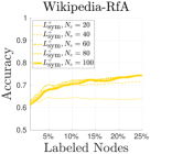
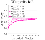
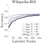
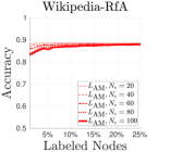
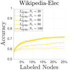
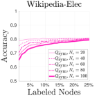
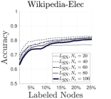
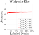
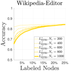
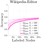
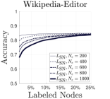
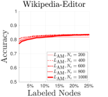
Figure 1: Average classification accuracy with different amounts of labeled nodes given a fixed number of eigenvectors. Each row presents classification accuracy of dataset Wikipedia-RfA, Wikipedia-Elec, and Wikipedia-Editor. Each column presents classification accuracy of GL($L_{\mathrm{sym}}^{+}$), GL($Q_{\mathrm{sym}}^{-}$), GL($L_{SN}$), and GL($L_{AM}$).

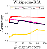
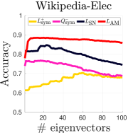
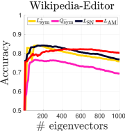
Figure 2: Average classification accuracy with $5\%$ labeled nodes and different amounts of eigenvectors. Average accuracy is computed out of 10 runs. Our method based on Laplacians $L_{\textrm{SN}}$ and $L_{\textrm{AM}}$ consistently presents the best classification performance.

4.3 Effect of the Number of Labeled Nodes

We now study how the classification accuracy of our method is affected by the amount of labeled nodes. For our method we fix the number of eigenvectors to $N_{e}\in\{20,40,60,80,100\}$ for Wikipedia-RfA and Wikipedia-Elec, and $N_{e}\!\in\!\{200,400,600,800,1000\}$ for Wikipedia-Editor. Given $N_{e}$, we evaluate our method with different proportions of labeled nodes, going from $1\%$ to $25\%$ of the number of nodes $\left|V\right|$. The corresponding average classification accuracy is shown in Fig. 1. As expected, we can observe that the classification accuracy increases with larger amounts of labeled nodes. Further, we can observe that this effect is more pronounced when larger amounts of eigenvectors $N_{e}$ are taken, i.e. the smallest classification accuracy increment is observed when the number of eigenvectors $N_{e}$ is $20$ for Wikipedia-RfA and Wikipedia-Elec and $100$ eigenvectors for Wikipedia-Editor. Further, we can observe that overall our method based on GL($L_{SN}$) and GL($L_{AM}$) performs best, suggesting that blending the information coming from both positive and negative edges is beneficial for the task of node classification. While our method based on signed Laplacians GL($L_{SN}$) and GL($L_{AM}$) overall presents the best performance, we can observe that they present a slightly difference when it comes to its sensibility to the amount of labeled nodes. In particular, we can observe how the increment on classification accuracy GL($L_{SN}$) is rather clear, whereas with GL($L_{AM}$) the increment is smaller. Yet, GL($L_{AM}$) systematically presents a better classification accuracy when the amount of labeled nodes is limited.

4.4 Effect of the Number of Eigenvectors

We now study how the performance of our method is affected by the number of eigenvectors given through different Laplacians. We fix the amount of labeled nodes to $5\%$ and consider different amounts of given eigenvectors. For datasets Wikipedia-RfA and Wikipedia-Elec we set the number of given eigenvectors $N_{e}$ in the range $N_{e}=1,\ldots,100$ and for Wikipedia-Editor in the range $N_{e}=1,10,\ldots,1000$. The average classification accuracy is shown in Fig. 2. For Wikipedia-RfA and Wikipedia-Elec we can see that the classification accuracy of our method based on GL($Q^{-}_{\mathrm{sym}}$) outperforms our method based on the Laplacian GL($L^{+}_{\mathrm{sym}}$) by a meaningful margin, suggesting that for the task of node classification negative edges are more informative than positive edges. Further, we can see that GL($L_{\text{AM}}$) consistently shows the highest classification accuracy indicating that taking into account the information coming from both positive and negative edges is beneficial for classification performance. For the case of Wikipedia-Editor the previous distinctions are not clear anymore. For instance, we can see that the performance of our method based on the Laplacian GL($L^{+}_{\mathrm{sym}}$) outperforms the case with GL($Q^{-}_{\mathrm{sym}}$). Moreover, the information coming from positive edges presents a more prominent performance, being competitive to our method based on the Laplacian GL($L_{\text{SN}}$) when the number of eigenvectors is relatively small, whereas the case with the arithmetic mean Laplacian GL($L_{\text{AM}}$) presents a larger classification accuracy for larger amounts of eigenvectors. Finally, we can see that in general our method first presents an improvement in classification accuracy, reaches a maximum and then decreases with the amount of given eigenvectors.

4.5 Joint Effect of the Number of Eigenvectors and Labeled Nodes

We now study the joint effect of the number of eigenvectors and the amount of labeled nodes in the classification performance of our method based on GL($L_{\text{SN}}$). We let the number of eigenvectors $N_{e}\in\{10,20,\ldots,100\}$ for datasets Wikipedia-RfA and Wikipedia-Elec and $N_{e}\in\{100,200,\ldots,1000\}$ for dataset Wikipedia-Editor. Further, we let the amount of labeled nodes to go from $1\%$ to $25\%$. The corresponding results are shown in Fig. 3, where we confirm that the classification accuracy consistently increases with larger amounts of labeled nodes. Finally, we can notice that the classification accuracy first increases with the amount of eigenvectors, it reaches a maximum, and then slightly decreases. To better appreciate the performance of our method under various settings, we present the difference between the lowest and largest average classification accuracy in the bottom table of Fig. 3. We can see that the increments go from $25.13\%$ to $36.54\%$.

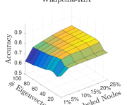
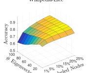
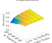
Dataset	Lowest Accuracy	Largest Accuracy	Increment
wikipedia-Elec	0.6317	0.8625	36.54$\%$
wikipedia-RfA	0.6264	0.8280	32.17$\%$
wikipedia-Editor	0.6785	0.8491	25.13$\%$

Figure 3: Top: Average classification accuracy of our method with GL($L_{SN}$) under different number of eigenvectors and different amounts of labeled nodes. Bottom: Lowest and largest average classification accuracy of GL($L_{\text{SN}}$) per dataset.

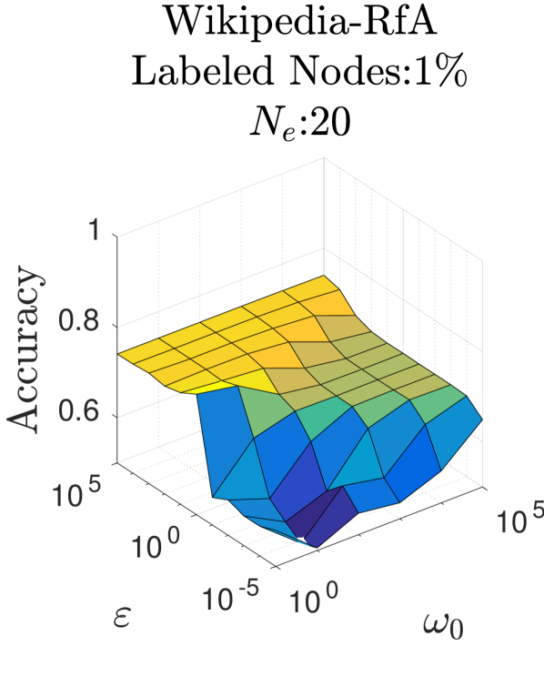
(a)

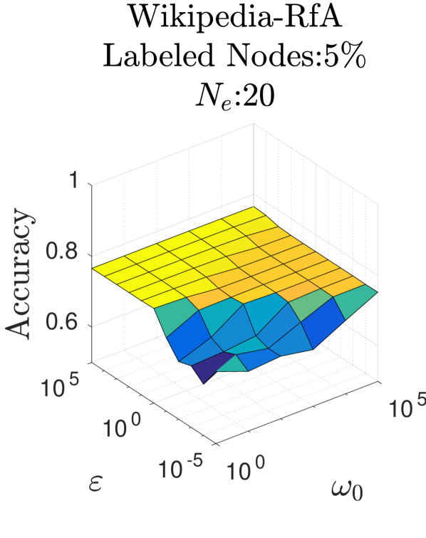
(b)

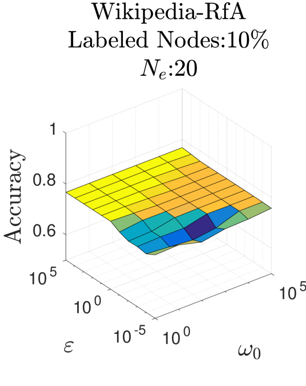
(c)

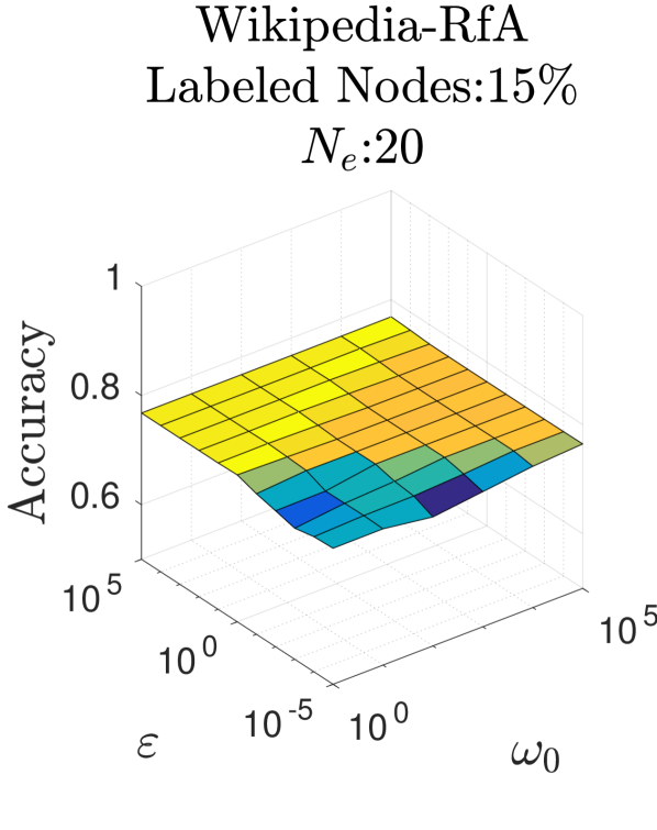
(d)

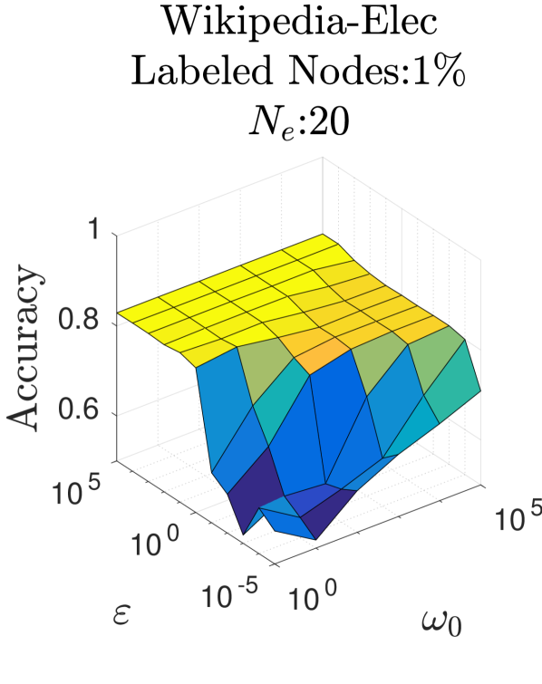
(e)

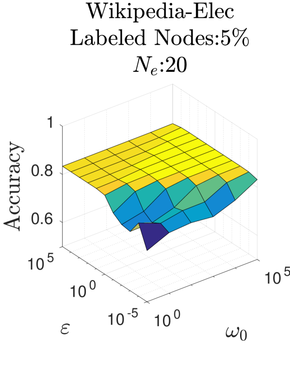
(f)

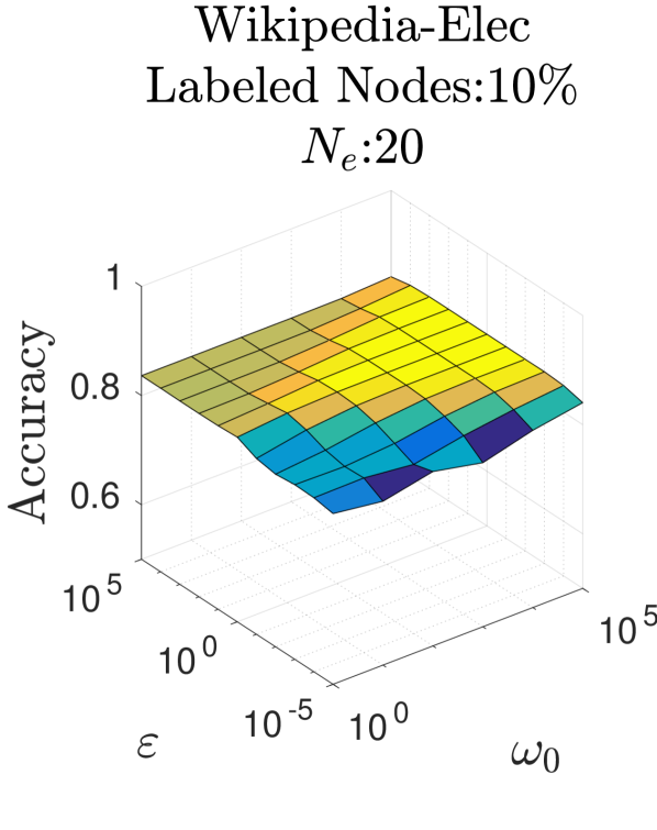
(g)

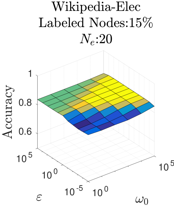
(h)

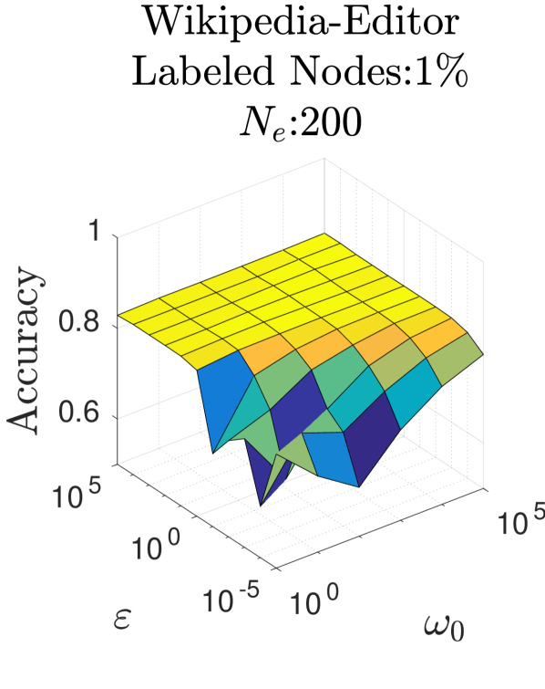
(i)

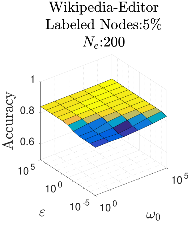
(j)

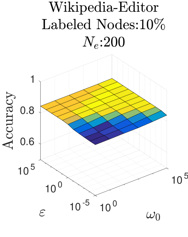
(k)

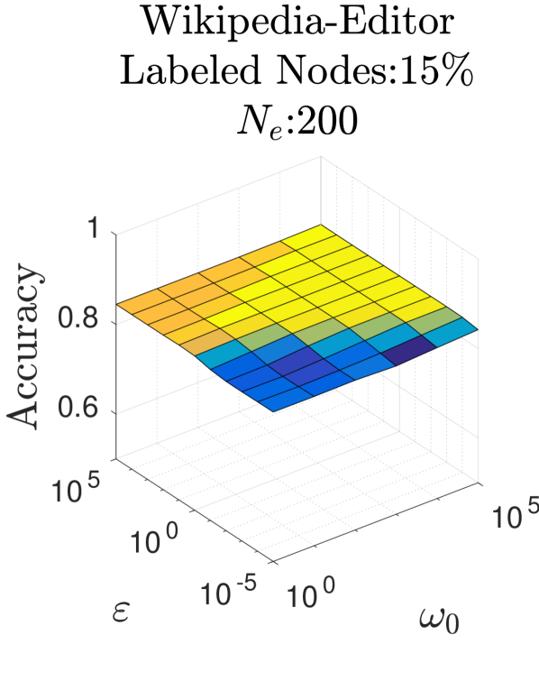
(l)

Figure 4: Average classification accuracy of our method based on GL($L_{SN}$) with different values of fidelity ($\omega_{0}$) and interface ($\varepsilon$). Columns (from left to right): amount of labeled nodes: $1\%,5\%,10\%,15\%$. Rows (from top to bottom): classification accuracy on datasets Wikipedia-RfA, Wikipedia-Elec, and Wikipedia-Editor.

4.6 Joint effect of fidelity ($\omega_{0}$) and interface ($\varepsilon$) parameters

We now study the effect of fidelity ($\omega_{0}$) and interface ($\varepsilon$) parameters on the classification accuracy of our method based on GL($L_{SN}$). We fix the number of eigenvectors to $N_{e}=20$, and let the amount of labeled nodes to go from $1\%$ to $15\%$. Further, we set the fidelity parameter $\omega_{0}$ to take values in $\{10^{0},10^{1},\ldots,10^{5}\}$ and the interface parameter $\varepsilon$ to take values in $\{10^{-5},10^{-4},\ldots,10^{4},10^{5}\}$. The results are shown in Fig. 4. We present the following observations: First: we can see that the larger the amount of labeled nodes, the smaller is the effect of parameters $(\omega_{0},\varepsilon)$. In particular, we can observe that when the amount of labeled nodes is at least $10\%$ of the number of nodes, then the parameter effect of $(\omega_{0},\varepsilon)$ is small, in the sense that the classification accuracy remains high. Second: we can see that there is a relationship between the fidelity parameter $\omega_{0}$ and the interface parameter $\varepsilon$ describing a safe region, in the sense that the classification accuracy is not strongly affected by the lack of large amounts of labeled nodes. In particular, we can observe that this region corresponds to the cases where the interface parameter $\varepsilon$ is larger than the fidelity parameter $\omega_{0}$, i.e. $\varepsilon(k_{1})>\omega_{0}(k_{2})$ where $\varepsilon(k_{1})=10^{k_{1}}$ and $\omega_{0}(k_{2})=10^{k_{2}}$, with $k_{1}\in\{10^{0},10^{1},\ldots,10^{5}\}$ and $k_{2}\in\{10^{-5},10^{-4},\ldots,10^{4},10^{5}\}$. This can be well observed through a slightly triangular region particularly present for the case where the amount of labeled nodes is $1\%$ on all datasets, which is depicted in Figs. 4(a), 4(e), and 4(i) .

5 Conclusion

We have illustrated that the semi-supervised task of node classification in signed networks can be performed via a natural extension of diffuse interface methods by taking into account suitable signed graph Laplacians. We have shown that different signed Laplacians provide different classification performances under real world signed networks. In particular, we have observed that negative edges provide a relevant amount of information, leading to an improvement in classification performance when compared to the unsigned case. As future work the task of non-smooth potentials can be considered, together with more diverse functions of matrices that would yield different kinds of information merging of both positive and negative edges.

6 Vector-valued formulation

This section contains further details of multi-class case of the approach proposed in Section 3. Garcia-Cardona et al. [25] as well as Merkurjev et al. [44] have extended the use of the diffuse interface model based on the generalized Ginzburg–Landau energy to multi-class segmentation of high-dimensional data on graphs. For hypergraphs this was done in [7]. We introduce the matrix $U=({u}_{1},\ldots,{u}_{n})^{T}\in\mathbb{R}^{n\times K}$, where the $m$th component of the vector ${u}_{i}\in\mathbb{R}^{K}$ indicates the strength for data point or graph vertex $i$ to belong to class $m$. Interpreting this is the sense of a probability distribution for vertex $i$ belonging to class $m,$ we need to make sure that the sum of the entries in one row will sum to one. For this we now for each node $i$ force the vector ${u}_{i}$ to be an element of the Gibbs simplex $\Sigma^{K}$

$$\Sigma^{K}:=\left\{(x_{1},\ldots,x_{K})^{T}\in[0,1]^{K}\left|\,\sum_{l=1}^{K}{x_{l}}=1\right.\right\}.$$

The vector-valued Ginzburg–Landau energy functional on graphs as in Section  3 of the main paper generalizes to the multi-class case as

$$E(U)=\frac{\varepsilon}{2}\textup{trace}(U^{T}SU)+\frac{1}{2\varepsilon}\sum_{i\in V}{\left(\prod_{l=1}^{K}{\frac{1}{4}||{u}_{i}-{\bf e}_{l}}||_{L_{1}}^{2}\right)}+\sum_{i\in V}{\frac{\omega_{i}}{2}||\hat{u}_{i}-{u}_{i}||^{2}_{L_{2}}}.$$ (4)

Let us explain this energy in more detail. We again have an energy term given by

$$\frac{\varepsilon}{2}\textup{trace}(U^{T}SU),$$

which again induces smoothness and adds clustering information to the functional. The role played by this part mirrors the energy term $\frac{\varepsilon}{2}u^{T}Su$ for the binary classification problem. The vector-valued potential

$$\frac{1}{2\varepsilon}\sum_{i\in V}{\left(\prod_{l=1}^{K}{\frac{1}{4}||{u}_{i}-{\bf e}_{l}}||_{L_{1}}^{2}\right)}$$

enforces that the components of $U$ are either $0$ or $1$. The term that incorporates the already labeled information is here

$$\sum_{i\in V}{\frac{\omega_{i}}{2}||\hat{u}_{i}-{u}_{i}||^{2}_{L_{2}}}$$

with $\omega_{i}$ the penalty parameter analogous to the two-classes classification case and with $\hat{U}=(\hat{u}_{1},\ldots,\hat{u}_{n})^{T}$ representing the already labeled data. Here, ${\bf e}_{l}\in\mathbb{R}^{K}$ being the vector whose $l$-th component equals one and all other components vanish. Note that the vectors ${\bf e}_{1},\ldots,{\bf e}_{K}$ correspond to the perfect classification outcome. The authors in [25, 44] use an $L_{1}$-norm for the potential term (the middle term in (4)) since it prevents an undesirable minimum from occurring at the center of the simplex, as it would be the case with an $L_{2}$-norm for large $K$, so as to avoid an undesired and hence useless classification result. The same convexity splitting scheme as in Section 3 of the main is used to minimize the Ginzburg–Landau functional in the phase-field approach. This results in

$$\frac{U^{(t+1)}-U^{(t)}}{\tau}+\varepsilon SU^{(t+1)}+cU^{(t+1)}=-\frac{1}{2\varepsilon}T(U^{(t)})+cU^{(t)}+\omega(\hat{U}-U^{(t)}),$$ (5)

where the elements $T_{ik}$ of the matrix $T(U^{(t)})$ are given as

$$T_{ik}=\sum_{l=1}^{K}{\frac{1}{2}\left(1-2\delta_{kl}\right)||\bar{u}_{i}-{\bf e}_{l}||_{L_{1}}}\prod_{m=1,m\neq l}^{K}{\frac{1}{4}||\bar{u}_{i}-{\bf e}_{m}}||_{L_{1}}^{2},$$

which represents the derivative of the potential term. Note that $\omega$ is a diagonal matrix containing the $\omega_{1},\ldots\omega_{K}$. The parameter $c\geq\omega_{0}+\frac{1}{\varepsilon}$ arises from the convexity splitting. As before, we assume that $U$ is evaluated at the new time-point, whereas $U^{(t)}$ indicates the previous time-point. Using the eigendecomposition $S=\Phi\Lambda\Phi^{T}$ and multiplying (5) by $\Phi^{T}$ from the left, we obtain

$$\mathcal{U}^{(t+1)}=B^{-1}\left[(1+c\tau)\mathcal{U}^{(t)}-\frac{\tau}{2\varepsilon}\Phi^{T}T(U^{(t)})+\tau\omega(\hat{\mathcal{U}}-{\mathcal{U}^{(t)}})\right],$$ (6)

where the calligraphic fonts have the meaning $\mathcal{U}=\Phi^{T}U$, ignoring the superscript for the time-step, and $\hat{\mathcal{U}}=\Phi^{T}\hat{U}$. Since $B=(1+c\tau)I+\varepsilon\tau\Lambda$ is a diagonal matrix with positive entries, its inverse is easy to apply. After the update, we have to project the solution back to the Gibbs simplex $\Sigma^{K}$ for the variable $U$ to reflect a probability distribution indicating to which class the $i$-th vertex belongs. In order to do this, we make use of the projection procedure in [12]. For the initialization of the segmentation problem, we first assign random values from the standard uniform distribution on $(0,1)$ to the nodes. Then, we project the result to the Gibbs simplex $\Sigma^{K}$ and set the values in the labeled nodes.

References

- [1] Allen, S.M., Cahn, J.W.: A microscopic theory for antiphase boundary motion and its application to antiphase domain coarsening. Acta Metall. 27(6), 1085–1095 (1979)
- [2] Basu, S., Davidson, I., Wagstaff, K.: Constrained clustering: Advances in algorithms, theory, and applications. CRC Press (2008)
- [3] Belkin, M., Matveeva, I., Niyogi, P.: Regularization and semi-supervised learning on large graphs. In: COLT (2004)
- [4] Bertozzi, A.L., Esedoḡlu, S., Gillette, A.: Inpainting of binary images using the Cahn–Hilliard equation. IEEE Trans. Image Process. 16(1), 285–291 (2007)
- [5] Bertozzi, A.L., Flenner, A.: Diffuse interface models on graphs for classification of high dimensional data. Multiscale Model. Simul. 10(3), 1090–1118 (2012)
- [6] Blowey, J.F., Elliott, C.M.: Curvature dependent phase boundary motion and parabolic double obstacle problems. In: Degenerate diffusions, IMA Vol. Math. Appl., vol. 47, pp. 19–60. Springer (1993)
- [7] Bosch, J., Klamt, S., Stoll, M.: Generalizing diffuse interface methods on graphs: Nonsmooth potentials and hypergraphs. SIAM Journal on Applied Mathematics 78(3), 1350–1377 (2018)
- [8] Bosch, J., Kay, D., Stoll, M., Wathen, A.J.: Fast solvers for Cahn–Hilliard inpainting. SIAM J. Imaging Sci. 7(1), 67–97 (2014)
- [9] Cahn, J.W., Hilliard, J.E.: Free energy of a nonuniform system. I. Interfacial free energy. J. Chem. Phys. 28(2), 258–267 (1958)
- [10] Cartwright, D., Harary, F.: Structural balance: a generalization of Heider’s theory. Psychological Review 63(5), 277–293 (1956)
- [11] Chapelle, O., Schlkopf, B., Zien, A.: Semi-Supervised Learning. The MIT Press (2010)
- [12] Chen, Y., Ye, X.: Projection onto a simplex. ArXiv e-prints:1101.6081 (2011)
- [13] Chiang, K., Whang, J., Dhillon, I.: Scalable clustering of signed networks using balance normalized cut. pp. 615–624. CIKM (2012)
- [14] Chung, F., Tsiatas, A., Xu, W.: Dirichlet pagerank and ranking algorithms based on trust and distrust. Internet Mathematics 9(1), 113–134 (2013)
- [15] Cucuringu, M., Davies, P., Glielmo, A., Tyagi, H.: SPONGE: A generalized eigenproblem for clustering signed networks. AISTATS (2019)
- [16] Cucuringu, M., Pizzoferrato, A., van Gennip, Y.: An MBO scheme for clustering and semi-supervised clustering of signed networks. CoRR abs/1901.03091 (2019)
- [17] Davis, J.A.: Clustering and structural balance in graphs. Human Relations 20, 181–187 (1967)
- [18] Derr, T., Ma, Y., Tang, J.: Signed graph convolutional networks. In: ICDM (2018)
- [19] Desai, M., Rao, V.: A characterization of the smallest eigenvalue of a graph. Journal of Graph Theory 18(2), 181–194 (1994)
- [20] Doreian, P., Mrvar, A.: Partitioning signed social networks. Social Networks 31(1), 1–11 (2009)
- [21] Elliott, C.M., Stinner, B.: Modeling and computation of two phase geometric biomembranes using surface finite elements. J. Comput. Phys. 229(18), 6585–6612 (2010)
- [22] Eyre, D.J.: Unconditionally gradient stable time marching the Cahn–Hilliard equation. In: MRS Proceedings (1998)
- [23] Falher, G.L., Cesa-Bianchi, N., Gentile, C., Vitale, F.: On the Troll-Trust Model for Edge Sign Prediction in Social Networks. In: AISTATS (2017)
- [24] Gallier, J.: Spectral theory of unsigned and signed graphs. applications to graph clustering: a survey. arXiv preprint arXiv:1601.04692 (2016)
- [25] Garcia-Cardona, C., Merkurjev, E., Bertozzi, A.L., Flenner, A., Percus, A.G.: Multiclass data segmentation using diffuse interface methods on graphs. IEEE Trans. Pattern Anal. Mach. Intell. 36(8), 1600–1613 (2014)
- [26] Garcke, H., Nestler, B., Stinner, B., Wendler, F.: Allen-Cahn systems with volume constraints. Math. Models Methods Appl. Sci. 18(8), 1347–1381 (2008)
- [27] Garcke, H., Nestler, B., Stoth, B.: A multi phase field concept: Numerical simulations of moving phasee boundaries and multiple junctions. SIAM J. Appl. Math. 60, 295–315 (1999)
- [28] van Gennip, Y., Guillen, N., Osting, B., Bertozzi, A.L.: Mean curvature, threshold dynamics, and phase field theory on finite graphs. Milan J. Math. 82(1), 3–65 (2014)
- [29] Goldberg, A.B., Zhu, X., Wright, S.: Dissimilarity in graph-based semi-supervised classification. In: AISTATS (2007)
- [30] Harary, F.: On the notion of balance of a signed graph. Michigan Mathematical Journal 2, 143–146 (1953)
- [31] Kim, J., Park, H., Lee, J.E., Kang, U.: Side: Representation learning in signed directed networks. In: WWW (2018)
- [32] Kirkley, A., Cantwell, G.T., Newman, M.E.J.: Balance in signed networks. Phys. Rev. E 99 (Jan 2019)
- [33] Kumar, S., Spezzano, F., Subrahmanian, V.: Vews: A wikipedia vandal early warning system. In: KDD. ACM (2015)
- [34] Kumar, S., Spezzano, F., Subrahmanian, V., Faloutsos, C.: Edge weight prediction in weighted signed networks. In: ICDM (2016)
- [35] Kunegis, J., Schmidt, S., Lommatzsch, A., Lerner, J., Luca, E., Albayrak, S.: Spectral analysis of signed graphs for clustering, prediction and visualization. In: ICDM. pp. 559–570 (2010)
- [36] Leskovec, J., Huttenlocher, D., Kleinberg, J.: Predicting positive and negative links in online social networks. In: WWW. pp. 641–650 (2010)
- [37] Leskovec, J., Krevl, A.: SNAP Datasets: Stanford Large Network Dataset Collection. http://snap.stanford.edu/data (Jun 2014)
- [38] Liu, S.: Multi-way dual cheeger constants and spectral bounds of graphs. Advances in Mathematics 268, 306 – 338 (2015)
- [39] Luo, X., Bertozzi, A.L.: Convergence analysis of the graph Allen–Cahn scheme. Tech. rep., UCLA (2016)
- [40] Luxburg, U.: A tutorial on spectral clustering. Statistics and Computing 17(4), 395–416 (Dec 2007)
- [41] Mercado, P., Gautier, A., Tudisco, F., Hein, M.: The power mean laplacian for multilayer graph clustering. In: AISTATS (2018)
- [42] Mercado, P., Tudisco, F., Hein, M.: Clustering signed networks with the geometric mean of Laplacians. In: NIPS (2016)
- [43] Mercado, P., Tudisco, F., Hein, M.: Spectral clustering of signed graphs via matrix power means. In: ICML (2019)
- [44] Merkurjev, E., Garcia-Cardona, C., Bertozzi, A.L., Flenner, A., Percus, A.G.: Diffuse interface methods for multiclass segmentation of high-dimensional data. Appl. Math. Lett. 33, 29–34 (2014)
- [45] Newman, M.E.J.: Modularity and community structure in networks. Proceedings of the National Academy of Sciences 103(23), 8577–8582 (2006)
- [46] Schönlieb, C.B., Bertozzi, A.L.: Unconditionally stable schemes for higher order inpainting. Commun. Math. Sci 9(2), 413–457 (2011)
- [47] Sedoc, J., Gallier, J., Foster, D., Ungar, L.: Semantic word clusters using signed spectral clustering. In: ACL (2017)
- [48] Serafino, F., Pio, G., Ceci, M.: Ensemble learning for multi-type classification in heterogeneous networks. IEEE TKDE (2018)
- [49] Shahriari, M., Jalili, M.: Ranking nodes in signed social networks. Social Network Analysis and Mining 4(1), 172 (Jan 2014)
- [50] Tang, J., Aggarwal, C., Liu, H.: Node classification in signed social networks. In: SDM (2016)
- [51] Tang, J., Chang, Y., Aggarwal, C., Liu, H.: A survey of signed network mining in social media. ACM Comput. Surv. 49(3), 42:1–42:37 (Aug 2016)
- [52] Tang, W., Lu, Z., Dhillon, I.S.: Clustering with multiple graphs. In: ICDM (2009)
- [53] Taylor, J.E., Cahn, J.W.: Linking anisotropic sharp and diffuse surface motion laws via gradient flows. J. Statist. Phys. 77(1-2), 183–197 (1994)
- [54] Tudisco, F., Mercado, P., Hein, M.: Community detection in networks via nonlinear modularity eigenvectors. SIAM Journal on Applied Mathematics 78(5), 2393–2419 (2018)
- [55] Wang, S., Tang, J., Aggarwal, C., Chang, Y., Liu, H.: Signed network embedding in social media. In: SDM (2017)
- [56] Wang, X., Du, Q.: Modelling and simulations of multi-component lipid membranes and open membranes via diffuse interface approaches. J. Math. Biol. 56(3), 347–371 (2008)
- [57] Yuan, S., Wu, X., Xiang, Y.: SNE: Signed network embedding. In: PAKDD (2017)
- [58] Zhou, D., Bousquet, O., Lal, T.N., Weston, J., Schölkopf, B.: Learning with local and global consistency. In: NIPS (2003)
- [59] Zhou, D., Burges, C.J.: Spectral clustering and transductive learning with multiple views. In: ICML (2007)
- [60] Zhu, X., Ghahramani, Z., Lafferty, J.: Semi-supervised learning using gaussian fields and harmonic functions. In: ICML (2003)
- [61] Zhu, X., Goldberg, A.B.: Introduction to semi-supervised learning. Synthesis Lectures on Artificial Intelligence and Machine Learning 3(1) (2009)