Spatial Variable Selection and An Application to Virginia Lyme Disease Emergence

Abstract

Lyme disease is an infectious disease that is caused by a bacterium called Borrelia burgdorferi sensu stricto. In the United States, Lyme disease is one of the most common infectious diseases. The major endemic areas of the disease are New England, Mid-Atlantic, East-North Central, South Atlantic, and West North-Central. Virginia is on the front-line of the disease’s diffusion from the northeast to the south. One of the research objectives for the infectious disease community is to identify environmental and economic variables that are associated with the emergence of Lyme disease. In this paper, we use a spatial Poisson regression model to link the spatial disease counts and environmental and economic variables, and develop a spatial variable selection procedure to effectively identify important factors by using an adaptive elastic net penalty. The proposed methods can automatically select important covariates, while adjusting for possible spatial correlations of disease counts. The performance of the proposed method is studied and compared with existing methods via a comprehensive simulation study. We apply the developed variable selection methods to the Virginia Lyme disease data and identify important variables that are new to the literature. Supplementary materials for this paper are available online.

Key Words: Gaussian Process; GLMM; Multicollinearity; Poisson Regression; Spatial Count Data; Spatial Correlation.

1 Introduction

Lyme disease is one of the most commonly reported vector-borne diseases in the United States. The disease was first identified in 1975 in the town of Old Lyme, Connecticut, and was therefore named Lyme disease. Lyme disease is caused by the bacterium Borrelia burgdorferi sensu stricto. Through Ixodid species tick bites, the bacterium is transmitted to humans. Early symptoms of Lyme disease includes skin rash, fever, headache, and fatigue. If the patients are not treated during the early stage of infection, severe and chronic symptoms can occur. Those chronic symptoms include arthritis in major joints, shooting pains, numbness in the hands or feet, and memory problems. Based on Maes1998, the estimated treatment costs for the disease were around $2.5 billion over a five-year period, which is a significant public health burden. Thus, the study of Lyme disease emergence is of general interest in public health.

Although New England and other northeastern states are the initial endemic area for the disease, the endemic area has expanded over the last several decades, and Virginia is currently at its southward front line. Lyme disease spread from the northern part of Virginia to the southwestern part over the past decade, and the state also experienced an increasing number of cases. This makes Virginia an ideal state to study the mechanism behind the disease and discover crucial factors associated with emergence of Lyme disease. Because the transmission of Lyme disease involves tick bites, which are related to both environmental and human factors, one of the important research questions in Lyme disease study is to identify possible environmental and demographic factors that can contribute to the emergence of the disease.

The main objective of this paper is to develop a method to identify a subset of the explanatory variables that are important for the case counts of Lyme disease based on Virginia data. As we can see from Lyme disease data (more details will be described in Section 2), there exist spatial correlations among disease counts, and there is also strong multicollinearity among explanatory variables. Variable selection while accounting for spatial dependence and multicollinearity is a challenging aspect. In the Lyme disease literature, the basic statistical models such as the Poisson regression are often used for modeling disease counts, without consideration of spatial correlation. When the goal is to identify important covariates, simple analyses such as bivariate analyses were used (e.g., Allan2003, and Jackson2006). The proposed methods in this paper will enable automatic variable selection while accounting for spatial correlation. Methodologically, the present work provides the Lyme disease research community more sophisticated analytic tools for statistical modeling and analysis. To the best of our knowledge, this paper is the first work that uses statewide Lyme disease data and covariates at census tract level to identify important environmental and human factors involved in the disease’s spread.

Spatial data modeling, which has broad applications in ecology, epidemiology, agriculture, sociology, and other areas, has attracted great attention in recent years in the statistical literature. For spatial data, correlations among observations in near locations are typically nonnegligible, and one way to model the spatial correlations among locations is through random effects. For example, DiggleMoyeedTawn1998, and Zhang2002 employed generalized linear mixed models (GLMM) for spatial data with non-Gaussian outcomes. Various approaches to estimate the parameters in GLMM have been developed. An overview on current methods can be found in McCullochSearleNeuhaus2008.

Regarding variable selections, a wide class of variable selection approaches have been developed via shrinkage methods. The least absolute shrinkage and selection operator (LASSO) penalty is studied in Tibshirani1996 to solve the regression type problem. It is shown that LASSO does parameter estimation and variable selection simultaneously due to the shrinkage property of the $L_{1}$ penalty. The ridge penalty introduced in HorelKennard1970 always includes all the covariates. If there is a group of highly correlated covariates, the ridge penalty shrinks coefficients to each other but not to zero. Conversely, LASSO picks one covariate and assigns all weights to this covariate. In other words, ridge penalty tends to select the entire group, while LASSO tends to randomly pick only one covariate (Tibshirani1996). ZouHastie2005 proposed the elastic net penalty, which is a linear combination of the LASSO penalty and the ridge penalty. For a group of highly correlated covariates, the ridge and LASSO combination results in the trend of in and out together. Thus, the elastic net penalty has the property of automatic variable selection and continuous shrinkage. LASSO does not have the oracle property and can be inconsistent unless certain conditions are satisfied. In light of these drawbacks of LASSO, the adaptive LASSO (Zou2006) and adaptive elastic net (ZouZhang2009) were developed. In addition, FanLi2001 developed the smoothly clipped absolute deviation (SCAD) penalty. One may refer to FanLv2010 for a comprehensive review of variable selection methods. In addition to the above work, Bayesian methods are also popular for variable selection. A review and comparison of Bayesian variable selection methods is available in OharaSillanpaa2009.

In terms of implementation, Efronetal2004 proposed the least-angle regression (LARS) method to efficiently calculate the solution path of LASSO penalty in linear models. ParkHastie2007 extended the concept of the LARS algorithm to generalized linear models (GLM). An algorithm named elastic net penalized least squares (LARS-EN) in ZouHastie2005 is proposed for linear models with elastic net penalty. SchelldorferMeierBuhlmann2014 developed “GLMMLasso” for high-dimensional GLMM with LASSO penalty and the corresponding R package is named “glmmixedlasso” (glmmixedlasso). GrollTutz2014 also considered this type of problem and a gradient descent algorithm is proposed to maximize the penalized log-likelihood function with implementation in an R package “glmmLasso” (glmmLasso). A number of variable selection procedures for GLMM with longitudinal data settings are studied in Yang2007 and Cui2011. Besides, CaiDunson2006 proposed a fully Bayesian method to select fixed and random effects in the setting of GLMM. Ibrahimetal2011 selected both fixed and random effects in a general class of mixed effects models using maximum penalized likelihood estimation along with the SCAD and the adaptive LASSO penalty functions. YangZou2013 developed an generalized coordinate descent algorithm for computing the solution path of the hybrid Huberized support vector machine. BoehmVocketal2015 developed spatial variable selection methods using a spatially varying coefficients model and applied them to study the acute health effects of fine particular matter components.

Despite the rich literature in spatial data analysis and various developments in variable selections, there is still a gap in performing variable selection for spatially correlated responses and correlated covariates. Although the focus of the paper is in Lyme disease applications, the developed spatial variable selection methods and comparisons also contribute to the general statistical literature. Extensive simulations show that the performance of the proposed methods perform better than existing methods for spatially correlated responses and correlated covariates. We also use bootstrap to quantify the uncertainties in parameter estimations. An R package is developed to implement the proposed methods.

The rest of this paper is organized as follows. Section 2 introduces the Virginia Lyme disease data and the potential covariates for selection. Section 3 presents the spatial Poisson regression model with random effects and the computation of the likelihood function. Section 4 presents two customized estimation procedures for estimating model parameters and develops a bootstrap algorithm for constructing confidence intervals. Section 5 conducts simulations to study the performance of the developed methods in variable selections and compares with existing methods. Section 6 presents the data analysis for the Virginia Lyme data with interpretation and discussions. Section 7 contains conclusions and areas for future research.

2 Virginia Lyme Disease Data

The Lyme disease dataset for this paper contains case data from 2006 to 2011, and demographic data and land cover data in Virginia. Lyme disease case data were collected by the Virginia Department of Health (2006-VDH2006-2011). The demographic data (e.g., population density, median income, and average age) are from the 2010 census (Almquist2010). Land cover data were obtained from the Multi-Resolution Land Cover Consortium for 2006 (Fryetal2012). A more detailed explanation of the data sources is available in Seukepetal2015.

The Lyme disease cases were aggregated into census tracts for a couple of reasons: 1) the demographic information and land cover data are available for each census tract; and 2) the tract borders are based on certain features (e.g., rivers, roads) that are potential barriers to the movement of tick or other species involved in the Lyme disease transmission cycle (e.g., white-footed mice or deer). Figure 1(a) illustrates the Virginia study area and the locations of census centroids as indicated by dots. The response of interest is the summary of case counts from 2006 and 2011 in each census tract. The total population counts in each census tract are included into the model as an offset term. Figure 2 shows the number of Lyme disease cases and incidence rates (i.e., the number of cases divided by the total population) for each census tract. A more detailed visualization of the Virginia Lyme disease data is available in Lietal2014.

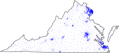
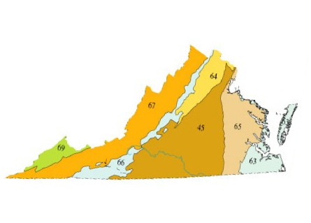
(a) Census Centroids	(b) Ecoregions

Figure 1: (a) Illustrations of the Virginia study area and the locations of census centroids as indicated by dots, and (b) the level III ecoregions from Ecoregions of Virginia (2015). The Subregion 1 ($\textrm{Eco\_id}=1$) represents the southern/eastern subregion, which includes Piedmont (code 45), Middle Atlantic Coastal Plain (code 63), and Southeastern Plains (code 65). The Subregion 0 ($\textrm{Eco\_id}=0$) represents northern/western subregion, which includes Northern Piedmont (code 64), Blue Ridge (code 66), Ridge and Valley (code 67), and Central Appalachian (code 69).

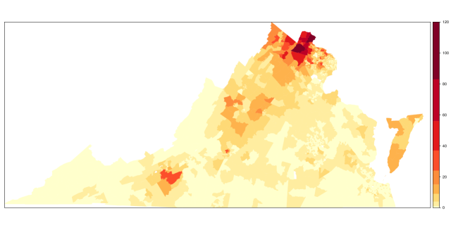
(a) Case counts.

(b) Incidence rates.

Figure 2: Number of cases and incidence rates of each census tract in Virginia for the five-year period (2006-2011). (a) Case counts. (b) Incidence rates.

Here, we discuss candidate covariates that may contribute to the case counts of Lyme disease. The summary of the candidate covariates is available in Table 1. The dissimilarities in economic and demographic characteristics may affect the incidence of Lyme disease. To understand the transmission of Lyme disease, it is important to study the environment of ticks and Lyme disease reservoirs.

In past studies, white-footed mice or deer are shown to be very important hosts of ticks. Forested and herbaceous/scrub areas are ideal habitats for white-footed mice or deer. According to Seukepetal2015, the herbaceous land type included scrub, herbaceous grasslands, cultivated agricultural lands, pasture, open impervious space, and emergent herbaceous wetlands. For example, scrub can provide tall enough vegetation to conceal deer and white-footed mice, and enough shade and humidity to allow black-legged ticks to survive the hot dry months of the summer. We consider four land cover types, which are the developed land, forest, herbaceous and water. The percentages of developed land, forest, and herbaceous within each tract are considered as covariates, with the percentage of water excluded because the percentages of those four land types add to 100%.

Allan2003 and Jackson2006 studied the effect of forest fragmentation on Lyme disease and showed that the percent of forested areas and number of small forest fragments ($<$2 ha) within each polygon are associated with incidence rate of Lyme disease. In this study, we consider two types of forest fragmentation variables: percent of small forest fragments ($<$2 ha) and percent of perimeters of the small forest fragments ($<$2 ha) within each census tract.

The mixture of land cover types can also be an important factor for the disease cases. For example, the boundary between forest and residential areas raises the risk for the interaction between tick or disease reservoirs and humans, which may lead to an increase in the incidence rate. In this study, we consider three types of edges of land covers, which are the developed-forest edge, the forest-herbaceous edge, and the herbaceous-developed edge. For each edge, we consider two types of indices that characterize the mixture of land cover types: Contrast Weighted Edge Density (CWED) and Total Edge Contrast Index (TECI), which represent two different algorithms for computing the mixture indices used in FRAGSTATS 4.1 (McGarigaletal2012).

We also consider the type of ecoregion in our analysis. Based on the level III ecoregion map of Virginia EcoregionVA, Virginia can be divided into two major subregions, representing environmental and demographic differences. Figure 1(b) illustrates the level III Ecoregions of Virginia. Subregion 1 (i.e., the southern/eastern subregion) consists of Piedmont, Middle Atlantic Coastal Plain, and Southeastern Plains areas, while Subregion 0 (i.e., the northern/western subregion) includes the Northern Piedmont, Blue Ridge, Ridge and Valley and Central Appalachian areas. In addition, the population density, median age, and mean income in 2010 are also included as potential factors in the study.

We observe multi-collinearity among the covariates in the data using the pairwise correlations among all the covariates. The range of the absolute values of the pairwise correlations is from 0.002 to 0.986. From Supplementary Figure 1, we can also see that the correlations among the covariates can go quite high (i.e., above 0.8), which motivates us to use the elastic-net type penalty in variable selection.

Table 1: Description of covariates in Lyme disease data.

Variable	Description
Dvlpd_NLCD06	Percentage of developed land in each census tract
Forest_NLCD06	Percentage of forest in each census tract
Herbaceous_NLCD06	Percentage of herbaceous in each census tract
Tract_Frag06	Sum of area of forested fragments in each census tract
	divided by the total area
FragPerim06	Sum of forest fragment perimeters in each census tract
	divided by the total area
CWED_DF06	CWED of developed-forest edge
TECI_DF06	TECI of developed-forest edge
CWED_FH06	CWED of forest-herbaceous edge
TECI_FH06	TECI of forest-herbaceous edge
CWED_HD06	CWED of herbaceous-developed edge
TECI_HD06	TECI of herbaceous-developed edge
Pop_den	Tract population density in 2010
Median_age	Median age at each census tract in 2010
Mean_income	Mean income (inflation adjusted) at each census tract
	in 2010
Eco_id	$\textrm{Eco\_id}=1$ represents the Piedmont, Middle Atlantic
	Coastal Plain, and Southeastern Plains areas; $\textrm{Eco\_id}=0$
	represents the Northern Piedmont, Blue Ridge, Ridge
	and Valley, and Central Appalachian areas

3 The Statistical Model

Here we introduce some notations about the spatial count data and covariates. Let $n$ be the number of spatial locations, which are indexed by $i=1,\ldots,n$. Let $Y_{i}$ be the random variable for the count of disease cases at location $i$, which takes values in $\{0,1,2,\ldots\}$. The corresponding observation is denoted by $y_{i}$. The explanatory variables at location $i$ are denoted by $\boldsymbol{x}_{i}=(x_{i1},\ldots,x_{ij},\ldots,x_{ip})^{\prime}$, where $p$ is the number of explanatory variables and $x_{ij}$ is the value of the $j$th covariate at location $i$. Let $\boldsymbol{y}=(y_{1},y_{2},\ldots,y_{n})^{\prime}$ be the vector of the observations, and $X$ be an $n\times p$ matrix for the explanatory variables. That is $X=(\boldsymbol{x}_{1},\ldots,\boldsymbol{x}_{i},\ldots,\boldsymbol{x}_{n})^{\prime}$. The population for location $i$ is denoted by $m_{i}$.

We use a spatial Poisson regression model with random effect $b_{i}$ to describe the spatial count data. That is,

$$Y_{i}|b_{i}\sim\textrm{Poisson}(\mu_{i}),$$ (1)

where

$$\eta_{i}=\log(\mu_{i})=\beta_{0}+x_{i1}\beta_{1}+\cdots+x_{ip}\beta_{p}+b_{i}+\log(m_{i}).$$

Here, $\mu_{i}$ is the conditional mean, $\eta_{i}$ is the log of $\mu_{i}$, $\beta_{j}$ is the regression coefficient of the corresponding covariate, and $\log(m_{i})$ is the offset term corresponding to the population for location $i$. The random effect is $b_{i}$. Given $b_{i}$, the probability mass function (pmf) of $Y_{i}$ is $\exp{(-\mu_{i})}\mu_{i}^{y_{i}}/y_{i}!$. The responses $Y_{i}$ are independent conditional on random effects $b_{i}$. Let $\boldsymbol{\mu}=(\mu_{1},\ldots,\mu_{n})^{\prime},{\boldsymbol{\beta}}=(\beta_{0},\beta_{1},\ldots,\beta_{p})^{\prime}$, and ${\boldsymbol{b}}=(b_{1},b_{2},\ldots,b_{n})^{\prime}$.

The spatial correlations among locations are captured through the random effects ${\boldsymbol{b}}$. Following the spatial literature, we use the multivariate normal distribution to model the random effect ${\boldsymbol{b}}$. That is,

$${\boldsymbol{b}}\sim\textrm{N}({\boldsymbol{0}},\Sigma_{{\boldsymbol{\theta}}}).$$ (2)

The variance-covariance matrix of ${\boldsymbol{b}}$ is $\Sigma_{{\boldsymbol{\theta}}}=\sigma^{2}\Omega$, and the $ij$th element of the $\Omega$ is $\rho(d_{ij};{\boldsymbol{\theta}})$. Here $\rho(\cdot)$ is a spatial correlation function and ${\boldsymbol{\theta}}$ are parameters in $\Sigma_{{\boldsymbol{\theta}}}$. Note that $d_{ij}$ is the distance between two locations $i$ and $j$. In this paper, the exponential correlation function is used. That is, $\rho(d_{ij};{\boldsymbol{\theta}})=\exp(-d_{ij}/d)$ and $d>0$ is the scale parameter. In this case, ${\boldsymbol{\theta}}=(\sigma^{2},d)^{\prime}$. The proposed method, however, can be extended to other spatial correlation functions such as the Gaussian, powered exponential, and Matérn correlation functions (e.g., Lietal2015).

Note that we use a distance-based correlation structure in (2). In some disease mapping and ecology applications, the Gaussian Markov random field is also used for the correlation structure. However, our problem is special in the sense that we use census tracts as our study units. As illustrated in Figure 1(a), some census tracts in southwest Virginia are relatively large while other census tracts in the northern Virginia area (outside Washington DC) are relatively small. If one uses a Markov random field, it would ignore the differences in distance among different census tracts. In addition, the transmission of Lyme disease is related to distance. Based on those considerations, we use a distance-based correlation structure in this paper.

Based on the model specification in (1) and (2), one can derive the likelihood function of unknown parameters ${\boldsymbol{\beta}}$ and ${\boldsymbol{\theta}}$. Specifically, let $f(\boldsymbol{y}|{\boldsymbol{\beta}},{\boldsymbol{b}})$ be the pmf of $\boldsymbol{y}$ given ${\boldsymbol{b}}$, and $f({\boldsymbol{b}}|{\boldsymbol{\theta}})$ be the probability density function (pdf) of ${\boldsymbol{b}}$. The likelihood function of $\{{\boldsymbol{\beta}},{\boldsymbol{\theta}}\}$ is

$$L({\boldsymbol{\beta}},{\boldsymbol{\theta}}) =\int_{\mathbb{R}^{n}}f(\boldsymbol{y}|{\boldsymbol{\beta}},{\boldsymbol{b}})f({\boldsymbol{b}}|{\boldsymbol{\theta}})\,d{\boldsymbol{b}}$$

$$=\int_{\mathbb{R}^{n}}\left[\prod\limits_{i=1}^{n}\exp{(-\mu_{i})}\dfrac{\mu_{i}^{y_{i}}}{y_{i}!}\right]\left[(2\pi)^{-\frac{n}{2}}|\Sigma_{{\boldsymbol{\theta}}}|^{-\frac{1}{2}}\exp{\left(-\frac{1}{2}{\boldsymbol{b}}^{\prime}\Sigma_{{\boldsymbol{\theta}}}^{-1}{\boldsymbol{b}}\right)}\right]\,d{\boldsymbol{b}}$$

$$=(2\pi)^{-\frac{n}{2}}|\Sigma_{{\boldsymbol{\theta}}}|^{-\frac{1}{2}}\int_{\mathbb{R}^{n}}\exp\left\{\sum\limits_{i=1}^{n}\left[-\mu_{i}+y_{i}\eta_{i}-\log(y_{i}!)\right]-\frac{1}{2}{\boldsymbol{b}}^{\prime}\Sigma_{{\boldsymbol{\theta}}}^{-1}{\boldsymbol{b}}\right\}\,d{\boldsymbol{b}},$$ (3)

where the integral of ${\boldsymbol{b}}$ is over the $n$-dimensional Euclidian space $\mathbb{R}^{n}$.

To perform variable selection, we add an adaptive elastic net (AEN) penalty term for fixed effects ${\boldsymbol{\beta}}$ to the log-likelihood function. That is, we consider the following penalized negative log-likelihood function

$$\mathcal{L}({\boldsymbol{\beta}},{\boldsymbol{\theta}})=-\log[L({\boldsymbol{\beta}},{\boldsymbol{\theta}})]+P_{{\boldsymbol{\lambda}}}({\boldsymbol{\beta}}),$$ (4)

where

$$P_{{\boldsymbol{\lambda}}}({\boldsymbol{\beta}})=\lambda_{1}\left[\lambda_{2}\sum_{j}\widehat{w}_{j}|\beta_{j}|+(1-\lambda_{2})\sum_{j}\beta_{j}^{2}\right]$$

is the AEN penalty. Here ${\boldsymbol{\lambda}}=(\lambda_{1},\lambda_{2})^{\prime}$ are regularization parameters. Note that $0\leqslant\lambda_{2}\leqslant 1$, $\lambda_{2}=1$ is the case of LASSO penalty, and $\lambda_{2}=0$ is the case of ridge penalty. In addition, $\widehat{w}_{j}=|\widehat{{\boldsymbol{\beta}}}_{\textrm{cnst}}|^{-r}$ is the adaptive weight with constant $r>0$, and $\widehat{{\boldsymbol{\beta}}}_{\textrm{cnst}}$ is an estimate of ${\boldsymbol{\beta}}$ that will be specified in Section 4.3.

Note that the likelihood function in (3) contains intractable integrals over distribution of random effects. If the random effects are of low dimension, we may use Gaussian quadrature to do numerical integration. However, in the spatial Poisson regression model with random effects, the dimension of random effects is often the same as the number of observations. That is, the dimension of integrals is typically so large that the Gaussian quadrature or other low-dimensional methods may not work well. Because the computation of the exact likelihood is infeasible, if not impossible, approximate likelihood is often used in literature, by employing the Laplace approximation. In particular, the Laplace approximation (Laplace1986) of multi-dimensional integrals over a multivariate function $\exp[h(\cdot)]$ is of the form

$$\int_{\mathbb{R}^{n}}\exp[h({\boldsymbol{b}})]\,d{\boldsymbol{b}}\approx(2\pi)^{\frac{n}{2}}\bigg{|}-h^{\prime\prime}(\widetilde{{\boldsymbol{b}}})\bigg{|}^{-\frac{1}{2}}\exp[h(\widetilde{{\boldsymbol{b}}})],$$

where $\widetilde{{\boldsymbol{b}}}$ is the maximizer of function $h({\boldsymbol{b}})$, and $\big{|}-h^{\prime\prime}(\widetilde{{\boldsymbol{b}}})\big{|}$ is the determinant of the negative of the Hessian matrix of $h(\cdot)$. For the likelihood function in (3), the corresponding $h(\cdot)$ function is

$$h({\boldsymbol{b}})=\sum_{i=1}^{n}\left[-\mu_{i}+y_{i}\eta_{i}-\log(y_{i}!)\right]-\frac{1}{2}{\boldsymbol{b}}^{\prime}\Sigma^{-1}{\boldsymbol{b}}.$$ (5)

Note that the maximizer $\widetilde{{\boldsymbol{b}}}$ of the function $h(\cdot)$ in (5) depends on parameters $\{{\boldsymbol{\beta}},{\boldsymbol{\theta}}\}$. Applying the Laplace approximation to likelihood function (3), we obtain

$$\log\left[L({\boldsymbol{\beta}},{\boldsymbol{\theta}})\right]\approx l({\boldsymbol{\beta}},{\boldsymbol{\theta}}),$$ (6)

where

$$l({\boldsymbol{\beta}},{\boldsymbol{\theta}})=-\frac{1}{2}\log\left(\big{|}\Sigma_{{\boldsymbol{\theta}}}W+I_{n}\big{|}\right)+\sum\limits_{i=1}^{n}\left[-\mu_{i}+y_{i}\eta_{i}-\log(y_{i}!)\right]-\frac{1}{2}\widetilde{{\boldsymbol{b}}}^{\prime}\Sigma_{{\boldsymbol{\theta}}}^{-1}\widetilde{{\boldsymbol{b}}},$$

is the log of the approximate likelihood function, $W=\textrm{Diag}\{\boldsymbol{\mu}\}$, and $I_{n}$ is an $n\times n$ identity matrix.

Thus, we use the following approximate penalized log-likelihood (APL) function to approximate the objective function in (4),

$$\mathcal{L}_{{\rm APL}}({\boldsymbol{\beta}},{\boldsymbol{\theta}})=-l({\boldsymbol{\beta}},{\boldsymbol{\theta}})+P_{{\boldsymbol{\lambda}}}({\boldsymbol{\beta}}).$$ (7)

The estimates of $\{{\boldsymbol{\beta}},{\boldsymbol{\theta}}\}$ can be obtained by finding the values of $\{{\boldsymbol{\beta}},{\boldsymbol{\theta}}\}$ that minimize the objective function in (7). An alternative approach from BreslowClayton1993 is to ignore the term $\big{|}\Sigma_{{\boldsymbol{\theta}}}W+I_{n}\big{|}$ in $l({\boldsymbol{\beta}},{\boldsymbol{\theta}})$, leading to the penalized quasi-likelihood (PQL) method. In particular, the PQL method aims to find the estimate of $\{{\boldsymbol{\beta}},{\boldsymbol{\theta}}\}$ by finding the values of $\{{\boldsymbol{\beta}},{\boldsymbol{\theta}}\}$ that minimize the following objective function,

$$\mathcal{L}_{{\rm PQL}}({\boldsymbol{\beta}},{\boldsymbol{\theta}})=-l_{a}({\boldsymbol{\beta}},{\boldsymbol{\theta}})+P_{{\boldsymbol{\lambda}}}({\boldsymbol{\beta}}),$$ (8)

where

$$l_{a}({\boldsymbol{\beta}},{\boldsymbol{\theta}})=\sum\limits_{i=1}^{n}\left[-\mu_{i}+y_{i}\eta_{i}-\log(y_{i}!)\right]-\frac{1}{2}\widetilde{{\boldsymbol{b}}}^{\prime}\Sigma_{{\boldsymbol{\theta}}}^{-1}\widetilde{{\boldsymbol{b}}}.$$ (9)

Essentially, the PQL uses $l_{a}({\boldsymbol{\beta}},{\boldsymbol{\theta}})$ to approximate $l({\boldsymbol{\beta}},{\boldsymbol{\theta}})$. Under the consideration of computation, the PQL method is more efficient, with the tradeoff of ignoring the dependency of $\Sigma_{{\boldsymbol{\theta}}}$ and $W$ on $\{{\boldsymbol{\beta}},{\boldsymbol{\theta}}\}$ in the expression $\big{|}\Sigma_{{\boldsymbol{\theta}}}W+I_{n}\big{|}$.

4 Parameter Estimation and Inference Procedures

In this section, we develop computational methods to optimize $\mathcal{L}_{{\rm APL}}({\boldsymbol{\beta}},{\boldsymbol{\theta}})$ and $\mathcal{L}_{{\rm PQL}}({\boldsymbol{\beta}},{\boldsymbol{\theta}})$ in (7) and (8), respectively. The developed estimation procedures are iterative. The goal is to estimate the unknown parameters ${\boldsymbol{\beta}}$ and ${\boldsymbol{\theta}}$. Both the APL and PQL methods share the following major steps:

• we first update $\widetilde{{\boldsymbol{b}}}$ based on the current estimates of ${\boldsymbol{\beta}}$ and ${\boldsymbol{\theta}}$,

• then update ${\boldsymbol{\beta}}$ with penalty $P_{{\boldsymbol{\lambda}}}({\boldsymbol{\beta}})$ to achieve variable selection, and

• finally update ${\boldsymbol{\theta}}$ based on the current estimates of ${\boldsymbol{\beta}}$ and $\widetilde{{\boldsymbol{b}}}$.

The above three-step procedure will be conducted iteratively until convergence. The details for the selection of tuning parameters ${\boldsymbol{\lambda}}$ are given in Section 4.3.

4.1 The APL Method

For the APL method, the first step is to find $\widetilde{{\boldsymbol{b}}}$ that maximizes $h({\boldsymbol{b}})$ in (5), given the current estimate of ${\boldsymbol{\beta}}$ and ${\boldsymbol{\theta}}$. Regular optimization methods such as the Newton-Raphson method can be used here. The second step is to use the block coordinate gradient descent (BCGD) method in TsengYun2009 to update ${\boldsymbol{\beta}}$ under penalty, given the current estimates of ${\boldsymbol{\beta}}$ and ${\boldsymbol{\theta}}$. The solution of an AEN penalty problem can be solved by transforming it into a LASSO type of problem. Specifically, minimizing (7) with respect to ${\boldsymbol{\beta}}$ is equivalent to minimizing

$$f({\boldsymbol{\beta}}|{\boldsymbol{b}},{\boldsymbol{\theta}})+\lambda_{1}\lambda_{2}\sum_{j}\widehat{w}_{j}|\beta_{j}|,$$

where

$$f({\boldsymbol{\beta}}|{\boldsymbol{b}},{\boldsymbol{\theta}})=\frac{1}{2}\log\left(\big{|}\Sigma_{{\boldsymbol{\theta}}}W+I_{n}\big{|}\right)-\sum\limits_{i=1}^{n}\left(-\mu_{i}+y_{i}\eta_{i}\right)+\frac{1}{2}{\boldsymbol{b}}^{\prime}\Sigma_{{\boldsymbol{\theta}}}^{-1}{\boldsymbol{b}}+\lambda_{1}(1-\lambda_{2})\sum_{j}\beta_{j}^{2}.$$ (10)

It is important to note that $f({\boldsymbol{\beta}}|{\boldsymbol{b}},{\boldsymbol{\theta}})$ is a non-convex but differentiable function, and $\sum_{j}\widehat{w}_{j}|\beta_{j}|$ is a convex but non-differentiable function. To apply the BCGD algorithm, we update only one component of ${\boldsymbol{\beta}}$ at a time. For the $j$th component of ${\boldsymbol{\beta}}$, denoted as $\beta_{j}$, we first obtain $\widetilde{{\boldsymbol{b}}}$ based on current estimates of ${\boldsymbol{\beta}}$ and ${\boldsymbol{\theta}}$, which are denoted by $\widetilde{{\boldsymbol{\beta}}}$ and $\widetilde{{\boldsymbol{\theta}}}$, respectively. Then we update the $j$th component by $\widetilde{\beta}_{j}+d_{j}$. Here,

$$d_{j}=\textrm{median}\left\{\dfrac{\widehat{w}_{j}\lambda_{1}\lambda_{2}-f_{j}(\widetilde{{\boldsymbol{\beta}}}|\widetilde{{\boldsymbol{b}}},\widetilde{{\boldsymbol{\theta}}})}{h_{jj}},\,\,-\widetilde{\beta}_{j},\,\,\dfrac{-\widehat{w}_{j}\lambda_{1}\lambda_{2}-f_{j}(\widetilde{{\boldsymbol{\beta}}}|\widetilde{{\boldsymbol{b}}},\widetilde{{\boldsymbol{\theta}}})}{h_{jj}}\right\}.$$

Also, $f_{j}({\boldsymbol{\beta}}|\widetilde{{\boldsymbol{b}}},\widetilde{{\boldsymbol{\theta}}})$ is the $j$th component of the first derivative of $f({\boldsymbol{\beta}}|\widetilde{{\boldsymbol{b}}},\widetilde{{\boldsymbol{\theta}}})$ with respect to ${\boldsymbol{\beta}}$ (i.e., $\partial f({\boldsymbol{\beta}}|\widetilde{{\boldsymbol{b}}},\widetilde{{\boldsymbol{\theta}}})/\partial{\boldsymbol{\beta}}$), and $h_{jj}$ is the $j$th diagonal element of $H$, where

$$\frac{\partial f({\boldsymbol{\beta}}|\widetilde{{\boldsymbol{b}}},\widetilde{{\boldsymbol{\theta}}})}{\partial{\boldsymbol{\beta}}} =X^{\prime}(\boldsymbol{\mu}-\boldsymbol{y})+2\lambda_{1}(1-\lambda_{2}){\boldsymbol{\beta}}+\boldsymbol{c},$$

$$H =X^{\prime}WX+2\lambda_{1}(1-\lambda_{2})I_{p}.$$

The $j$th element of $\boldsymbol{c}$ is $(1/2){\rm tr}\left\{(\Sigma_{{\boldsymbol{\theta}}}W+I_{n})^{-1}\Sigma_{{\boldsymbol{\theta}}}\partial W/\partial\beta_{j}\right\}$, and $I_{p}$ is a $p\times p$ identity matrix.

The last step of the iterative procedure is to update ${\boldsymbol{\theta}}$. The estimate of ${\boldsymbol{\theta}}$ is updated by minimizing (7) with current estimates $\widetilde{{\boldsymbol{\beta}}}$ and $\widetilde{{\boldsymbol{b}}}$. A description of the algorithm for the APL estimation procedure is as follows.
 
Algorithm 1: APL with Adaptive Elastic Penalty (APL.AEN)

For a collection of values of $(\lambda_{1},\lambda_{2})$:

1. Initialize ${\boldsymbol{\beta}}^{(0)},{\boldsymbol{b}}^{(0)}$, and ${\boldsymbol{\theta}}^{(0)}$.

2. For the $k$th iteration:

   1. To update the $j$th component of ${\boldsymbol{\beta}}$, one first finds $\widetilde{{\boldsymbol{b}}}^{(k,j)}$ that maximizes $h({\boldsymbol{b}})$ with given $\widetilde{{\boldsymbol{\beta}}}^{(k,j)}=(\widetilde{\beta}_{1}^{(k)},\ldots,\widetilde{\beta}_{j-1}^{(k)},\widetilde{\beta}_{j}^{(k-1)},\ldots,\widetilde{\beta}_{p}^{(k-1)})$ and $\widetilde{{\boldsymbol{\theta}}}^{(k-1)}$.

   2. Then update $\widetilde{\beta}_{j}^{(k)}=\widetilde{\beta}_{j}^{(k-1)}+d_{j}$.

   3. Repeat (i) and (ii) for $j=1,\ldots,p$.

   4. $\widetilde{{\boldsymbol{\theta}}}^{(k)}$ is obtained by minimizing (7) with $\widetilde{{\boldsymbol{\beta}}}^{(k)}$.

3. Repeat Step 2 until convergence. The final version of estimates $\widetilde{{\boldsymbol{\beta}}}$, $\widetilde{{\boldsymbol{b}}}$, and $\widetilde{{\boldsymbol{\theta}}}$ are denoted by $\widehat{{\boldsymbol{\beta}}},\widehat{{\boldsymbol{b}}},$ and $\widehat{{\boldsymbol{\theta}}}$, respectively.

4.2 The PQL Method

In this section we present how the parameters ${\boldsymbol{\beta}}$, ${\boldsymbol{\theta}}$, and ${\boldsymbol{b}}$ are sequentially updated in the PQL method. We use the iterative algorithm in BreslowClayton1993 to estimate $\{{\boldsymbol{\beta}},{\boldsymbol{b}}\}$ from (5). In particular, BreslowClayton1993 showed that the estimation of $\{{\boldsymbol{\beta}},{\boldsymbol{b}}\}$ is equivalently to fit a linear mixed model (LMM) as follows:

$$\boldsymbol{y}^{*}=X{\boldsymbol{\beta}}+{\boldsymbol{b}}+{\boldsymbol{\epsilon}},\textrm{ with }{\boldsymbol{b}}\sim\mathrm{N}({\boldsymbol{0}},\Sigma_{{\boldsymbol{\theta}}}),\textrm{ and }{\boldsymbol{\epsilon}}\sim\mathrm{N}({\boldsymbol{0}},W^{-1}).$$ (11)

Here $\boldsymbol{y}^{*}=(y_{1}^{*},\ldots,y_{n}^{*})$ is the working response vector with $y_{i}^{*}=\boldsymbol{x}_{i}^{\prime}{\boldsymbol{\beta}}+b_{i}+{(y_{i}-\mu_{i})}/{\mu_{i}}$. Based on the model formulation in (11), we obtain ${\rm Var}(\boldsymbol{y}^{*})=V=W^{-1}+\Sigma_{{\boldsymbol{\theta}}}$. We update $\widetilde{{\boldsymbol{\beta}}}$ and $\widetilde{{\boldsymbol{b}}}$ in the following formulas iteratively until convergence. In particular,

$$\widetilde{{\boldsymbol{\beta}}}=\left(X^{\prime}V^{-1}X\right)^{-1}X^{\prime}V^{-1}\boldsymbol{y}^{*},\quad\textrm{and}\quad\widetilde{{\boldsymbol{b}}}=\Sigma_{{\boldsymbol{\theta}}}V^{-1}\left(\boldsymbol{y}^{*}-X\widetilde{{\boldsymbol{\beta}}}\right).$$

The second step is to update ${\boldsymbol{\beta}}$ under penalty. To efficiently obtain one step update of ${\boldsymbol{\beta}}$ under the penalty, we use a quadratic approximation to $l_{a}({\boldsymbol{\beta}}|\widetilde{{\boldsymbol{b}}},\widetilde{{\boldsymbol{\theta}}})$, which is the $l_{a}({\boldsymbol{\beta}},{\boldsymbol{\theta}})$ in (9) but given $\widetilde{{\boldsymbol{\theta}}}$ and $\widetilde{{\boldsymbol{b}}}$. Note that $l_{a}({\boldsymbol{\beta}}|\widetilde{{\boldsymbol{b}}},\widetilde{{\boldsymbol{\theta}}})$ is a concave function of ${\boldsymbol{\beta}}$ given $\widetilde{{\boldsymbol{\theta}}}$ and $\widetilde{{\boldsymbol{b}}}$, and $\widetilde{{\boldsymbol{\beta}}}$ is the maximizer of $l_{a}({\boldsymbol{\beta}}|\widetilde{{\boldsymbol{b}}},\widetilde{{\boldsymbol{\theta}}})$. We form a quadratic approximation to $l_{a}({\boldsymbol{\beta}}|\widetilde{{\boldsymbol{b}}},\widetilde{{\boldsymbol{\theta}}})$ around $\widetilde{{\boldsymbol{\beta}}}$ to speed up the updating of ${\boldsymbol{\beta}}$. FriedmanHastieTibshirani2010 used a similar method for generalized linear models. In particular, we have

$$l_{a}({\boldsymbol{\beta}}|\widetilde{{\boldsymbol{\theta}}},\widetilde{{\boldsymbol{b}}})\approx-\dfrac{1}{2}\sum\limits_{i=1}^{n}\mu_{i}(z_{i}-\boldsymbol{x}_{i}^{\prime}{\boldsymbol{\beta}})^{2},$$

where $z_{i}=\boldsymbol{x}_{i}^{\prime}\widetilde{{\boldsymbol{\beta}}}-1+y_{i}/\mu_{i}$. The details regrading the derivation of the quadratic approximation is given in Appendix A. Incorporating the elastic net penalty function, we obtain

$$\mathcal{L}_{\textrm{PQL}}^{Q}({\boldsymbol{\beta}}|\widetilde{{\boldsymbol{\theta}}},\widetilde{{\boldsymbol{b}}})=\dfrac{1}{2}\sum\limits_{i=1}^{n}\mu_{i}(z_{i}-\boldsymbol{x}_{i}^{\prime}{\boldsymbol{\beta}})^{2}+P_{{\boldsymbol{\lambda}}}({\boldsymbol{\beta}}).$$ (12)

The minimizer $\widetilde{{\boldsymbol{\beta}}}_{Q}$ of (12) can be achieved as a penalized weighted least squares problem by using the R package “glmnet” (FriedmanHastieTibshirani2010).

It is interesting to point out that estimating ${\boldsymbol{\beta}}$ via optimizing (12) is equivalent to consider the penalized log-likelihood of the linear mixed model (11). That is,

$$-\frac{1}{2}(\boldsymbol{y}^{*}-X{\boldsymbol{\beta}}-{\boldsymbol{b}})^{\prime}W(\boldsymbol{y}^{*}-X{\boldsymbol{\beta}}-{\boldsymbol{b}})-\frac{1}{2}{\boldsymbol{b}}^{\prime}\Sigma_{{\boldsymbol{\theta}}}^{-1}{\boldsymbol{b}}-P_{{\boldsymbol{\lambda}}}({\boldsymbol{\beta}}).$$ (13)

To see the connection between (12) and (13), we estimate $\widetilde{{\boldsymbol{b}}}$ first and let $\boldsymbol{y}^{**}=\boldsymbol{y}^{*}-\widetilde{{\boldsymbol{b}}}$. Then again we have a weighted linear regression with elastic net penalty problem. That is we want to minimize

$$\frac{1}{2}\sum\limits_{i=1}^{n}\mu_{i}(y_{i}^{**}-\boldsymbol{x}_{i}^{\prime}{\boldsymbol{\beta}})^{2}+P_{{\boldsymbol{\lambda}}}({\boldsymbol{\beta}}),$$

which is equivalent to minimizing (12). That is, we can transform the GLMM with penalty problem into an LMM with penalty problem.

The last step of the iterative procedure is to update ${\boldsymbol{\theta}}$. We update ${\boldsymbol{\theta}}$ by using the restricted maximum likelihood (REML) method. The calculation of the REML function involves the elastic net penalty function $P_{{\boldsymbol{\lambda}}}({\boldsymbol{\beta}})$, which has the singularity at the origin. Therefore, we consider an approximation of the penalty function $P_{{\boldsymbol{\lambda}}}({\boldsymbol{\beta}})$. Based on FanLi2001, the penalty function $P_{{\boldsymbol{\lambda}}}({\boldsymbol{\beta}})$ can be approximated by

$$P_{{\boldsymbol{\lambda}}}({\boldsymbol{\beta}})\approx\frac{1}{2}\widetilde{{\boldsymbol{\beta}}}_{{\boldsymbol{\lambda}}}^{\prime}{\boldsymbol{\Sigma}}_{{\boldsymbol{\lambda}}}(\widetilde{{\boldsymbol{\beta}}}){\boldsymbol{\beta}}_{{\boldsymbol{\lambda}}},$$

where $\widetilde{{\boldsymbol{\beta}}}_{{\boldsymbol{\lambda}}}$ only contains nonzero elements $\widetilde{\beta}_{1},\ldots,\widetilde{\beta}_{m}$ of $\widetilde{{\boldsymbol{\beta}}}$, and

$${\boldsymbol{\Sigma}}_{{\boldsymbol{\lambda}}}(\widetilde{{\boldsymbol{\beta}}})=\textrm{Diag}\left\{\frac{P_{{\boldsymbol{\lambda}},\,\widetilde{\beta}_{1}}(|\widetilde{\beta}_{1}|)}{|\widetilde{\beta}_{1}|},\ldots,\frac{P_{{\boldsymbol{\lambda}},\,\widetilde{\beta}_{m}}(|\widetilde{\beta}_{m}|)}{|\widetilde{\beta}_{m}|}\right\}.$$

Here $P_{{\boldsymbol{\lambda}},\,\widetilde{\beta}_{j}}(|\widetilde{\beta}_{j}|)$ is the first partial derivative with respect to $\widetilde{\beta}_{j}$. Also, define $X_{{\boldsymbol{\lambda}}}$ to be the matrix corresponding to the nonzero elements of $\widetilde{{\boldsymbol{\beta}}}$. Cui2011 showed that the approximate REML estimator for ${\boldsymbol{\theta}}$ can be calculated by maximizing

$$-\frac{1}{2}\log|V|-\frac{1}{2}\log|X_{{\boldsymbol{\lambda}}}^{\prime}V^{-1}X_{{\boldsymbol{\lambda}}}+{\boldsymbol{\Sigma}}_{{\boldsymbol{\lambda}}}(\widetilde{{\boldsymbol{\beta}}})|-\frac{1}{2}\left(\boldsymbol{y}^{*}-X_{{\boldsymbol{\lambda}}}\widetilde{{\boldsymbol{\beta}}}_{{\boldsymbol{\lambda}}}\right)^{\prime}V^{-1}\left(\boldsymbol{y}^{*}-X_{{\boldsymbol{\lambda}}}\widetilde{{\boldsymbol{\beta}}}_{{\boldsymbol{\lambda}}}\right).$$ (14)

Note that the term ${\boldsymbol{\Sigma}}_{{\boldsymbol{\lambda}}}(\widetilde{{\boldsymbol{\beta}}})$ in $\log|X_{{\boldsymbol{\lambda}}}^{\prime}V^{-1}X_{{\boldsymbol{\lambda}}}+{\boldsymbol{\Sigma}}_{{\boldsymbol{\lambda}}}(\widetilde{{\boldsymbol{\beta}}})|$ is for adjustment of the penalty function of ${\boldsymbol{\beta}}$. Note that in alternative of maximizing the function in (14), expectation maximization (EM) type estimators can also be used (e.g., FahrmeirTutz2001, and GrollTutz2014). The estimation procedure is summarized in the following algorithm.

Algorithm 2: PQL with Adaptive Elastic Net Penalty (PQL.AEN)
For a collection of values of $(\lambda_{1},\lambda_{2})$:

1. Initialize ${\boldsymbol{\beta}}^{(0)},{\boldsymbol{b}}^{(0)}$, and ${\boldsymbol{\theta}}^{(0)}$.

2. For the $k$th iteration:

   1. Find $\{{\boldsymbol{\beta}},{\boldsymbol{b}}\}$ that maximize (5). Specifically, define the working response as

      $$\boldsymbol{y}^{*(k)}=\boldsymbol{x}_{i}^{\prime}\widetilde{{\boldsymbol{\beta}}}^{(k-1)}+\widetilde{{\boldsymbol{b}}}^{(k-1)}+{(\boldsymbol{y}-\widetilde{\boldsymbol{\mu}}^{(k-1)})}/{\widetilde{\boldsymbol{\mu}}^{(k-1)}},$$

      and update $\widetilde{{\boldsymbol{\beta}}}$ and $\widetilde{{\boldsymbol{b}}}$ iteratively until converge. The estimates obtained are denoted as $\widetilde{{\boldsymbol{\beta}}}^{(k)},\widetilde{{\boldsymbol{b}}}^{(k)}$.

   2. Given the current estimates $\widetilde{{\boldsymbol{\beta}}}^{(k)},\widetilde{{\boldsymbol{b}}}^{(k)},$ and $\widetilde{{\boldsymbol{\theta}}}^{(k-1)}$, solve

      $$\mathcal{L}_{\textrm{PQL}}^{Q}({\boldsymbol{\beta}}|\widetilde{{\boldsymbol{\theta}}}^{(k-1)},\widetilde{{\boldsymbol{b}}}^{(k)})=\dfrac{1}{2}\sum\limits_{i=1}^{n}\mu_{i}(z_{i}-\boldsymbol{x}_{i}^{\prime}{\boldsymbol{\beta}})^{2}+P_{{\boldsymbol{\lambda}}}({\boldsymbol{\beta}}),$$ (15)

      where $z_{i}$ and $\mu_{i}$ are evaluated at $\widetilde{{\boldsymbol{\beta}}}^{(k)},\widetilde{{\boldsymbol{b}}}^{(k)},$ and $\widetilde{{\boldsymbol{\theta}}}^{(k-1)}$. The estimate obtained is denoted by $\widetilde{{\boldsymbol{\beta}}}_{Q}^{(k)}$.

   3. Obtain the estimates of covariance parameters $\widetilde{{\boldsymbol{\theta}}}^{(k)}$ by maximizing (14) with $\widetilde{{\boldsymbol{\beta}}}_{Q}^{(k)}$ and $\widetilde{{\boldsymbol{b}}}^{(k)}$.

3. Repeat Step 2 until convergence. The final version of estimates $\widetilde{{\boldsymbol{\beta}}}_{Q}$, $\widetilde{{\boldsymbol{b}}}$, and $\widetilde{{\boldsymbol{\theta}}}$ are denoted by $\widehat{{\boldsymbol{\beta}}},\widehat{{\boldsymbol{b}}},$ and $\widehat{{\boldsymbol{\theta}}}$, respectively.

Both Algorithms 1 and 2 are implemented in R R2016 via an R package “SpatialVS” SpatialVS-Rpackage and a data package “VALymeData” SpatialVS-Datapackage. The Virginia Lyme disease data and the R code for simulation and analysis are also available via the online supplementary materials.

4.3 Specification of Adaptive Weights and Selection of Tuning Parameters

We need to specify the adaptive weights $\widehat{w}_{j}=|\widehat{{\boldsymbol{\beta}}}_{\textrm{cnst}}|^{-r}$ for the AEN penalty in (4). Following ZouZhang2009, we specify $\widehat{{\boldsymbol{\beta}}}_{\textrm{cnst}}$ to be the estimates under the elastic net penalty. For those elements of $\widehat{{\boldsymbol{\beta}}}_{\textrm{cnst}}$ that are set to zero by the elastic net penalty, we set them to be $1/n$ as in ZouZhang2009. We use $r=1$ in the simulation study and data analysis.

Regarding tuning parameters, popular methods of choosing the tuning parameters ${\boldsymbol{\lambda}}=(\lambda_{1},\lambda_{2})^{\prime}$ include cross-validation and criterion-based approaches. In this paper, we use the Bayesian Information Criterion (BIC) to select the tuning parameter. The calculation of exact log-likelihood for GLMM is complicated. Thus the Laplace approximated log-likelihood is used. For notation simplicity, we also use $\widehat{{\boldsymbol{\beta}}},\widehat{{\boldsymbol{b}}},$ and $\widehat{{\boldsymbol{\theta}}}$ to represent estimates obtained from penalized approximate likelihood. In particular, the BIC is defined by $-2l(\widehat{{\boldsymbol{\beta}}},\widehat{{\boldsymbol{\theta}}})+\log(n)df$, where $df$ is number of nonzero parameters in $\widehat{{\boldsymbol{\beta}}}$ plus the number of parameters in $\widehat{{\boldsymbol{\theta}}}$. The values of the tuning parameters ${\boldsymbol{\lambda}}=(\lambda_{1},\lambda_{2})^{\prime}$ are chosen to minimize the BIC.

Here we provide a brief discussion on the degrees of freedom (df) of the model. We use the number of nonzero parameters in $\widehat{{\boldsymbol{\beta}}}$ plus the number of parameters in $\widehat{{\boldsymbol{\theta}}}$ as the effective df, following SchelldorferMeierBuhlmann2014 and GrollTutz2014. The “real” complexity in GLMM is an open issue of current research. In particular, not only the number of random effects variance-covariance parameters but also their size has an influence on the model’s complexity. For example, if a random effect has a large variance, the corresponding random intercept or slope estimates are much larger and, the model tends to be more complex. Alternatively, the “glmmLasso” in glmmLasso allows to use the trace of the corresponding approximate hat matrix as model complexity.

4.4 Confidence Interval Procedures

In this section, we first review several existing methods for statistical inference of penalized models and then suggest to use parametric bootstrap to obtain confidence intervals (CIs) for parameters in the spatial model in this paper. FanLi2001 derived a sandwich-type standard error formula for nonzero components of the LASSO estimator. Zou2006 used a similar approach to derive the standard error formula for the nonzero components of the adaptive Lasso estimator. The sandwich-type estimator, however, can not provide uncertainty quantification for those zero components of the estimator. berk2013valid proposed a framework for valid post-selection inference by using simultaneous inference. Bachocetal2016 proposed a general method to construct asymptotically uniformly valid CIs post-model-selection using the principles in berk2013valid. lee2016exact developed a general approach for valid inference after model selection by characterizing the distribution of the post selection-estimator conditional on the selection event. lu2017confidence investigated the CI problem from a different point of view, and they used stochastic variational inequality techniques in optimization to derive CIs for the LASSO estimator. Overall, the current methodological developments are mostly made for LASSO type estimators.

ning2017general developed general theory for statistical inference for generic penalized M-estimator using the idea of decorrelated score function. Their approach is quite general and it can be applied to a variety of models such as linear models, generalized linear models, and survival models. Their approach can not be directly applied to our setting because all observations are correlated under the spatial model.

chatterjee2011bootstrapping showed that bootstrap methods are valid for the adaptive LASSO estimator due to its oracle property. For the AEN penalty, ZouZhang2009 showed that it also has oracle property under the setting of linear models. Although our setting is different, based on current methodological developments, a practical approach for constructing CIs for our model is the parametric bootstrap. One advantage of using the parametric bootstrap is that it can easily keep the spatial correlation in the bootstrapped samples. Thus, we use the parametric bootstrap to construct CIs in this paper. The detailed algorithm for the parametric bootstrap is available in Supplementary Section 2.

5 Simulation Studies

In this section, we evaluate the performance of the APL and PQL methods proposed in Sections 4.1 and 4.2, and compare with existing methods through simulations.

5.1 Simulation Setting

In the simulation study, we consider the following model:

$$y_{i}|b_{i}\sim\textrm{Poisson}\left[\exp(\boldsymbol{x}_{i}^{\prime}{\boldsymbol{\beta}}+b_{i})\right],$$

where $\boldsymbol{x}_{i}$ is the vector of covariates and ${\boldsymbol{\beta}}$ collects the corresponding coefficients. Here, the distribution of the random effect ${\boldsymbol{b}}$ is the same as in (2). That is the covariance has the form $(\Sigma_{{\boldsymbol{\theta}}})_{ij}=\sigma^{2}\exp(d_{ij}/d)$, where $d>0$ is the scale parameter. Each dataset consists of $n=225$ equal spaced data points that are simulated on a $[1,10]\times[1,10]$ regular grid. The distance between point $i$ and $j$ is denoted by $d_{ij}$. The $\boldsymbol{x}_{i}$ are simulated from multivariate normal distribution with mean $0$ and variance $0.5$.

We consider the following three settings of ${\boldsymbol{\beta}}$ and ${\boldsymbol{\theta}}$ to represent different degrees of covariate effects and the number of active (i.e., nonzero-effect) covariates:

(i) ${\boldsymbol{\beta}}=(-0.5,0.75,1,-0.75,-1,{\boldsymbol{0}}_{10})^{\prime}$, (ii) ${\boldsymbol{\beta}}=(0.2,0.3,0.4,0.5,0.7,0.8,-0.1,-0.6,-0.9,-1,{\boldsymbol{0}}_{10})^{\prime}$, (iii) ${\boldsymbol{\beta}}=(-0.5,0.75,1,-0.75,-1,{\boldsymbol{0}}_{20})^{\prime}$.

Here ${\boldsymbol{0}}_{n}$ is a vector of zeros with length $n$, and let $p$ represent the length of ${\boldsymbol{\beta}}$. The value of ${\boldsymbol{\theta}}=(\sigma^{2},d)^{\prime}$ is specified to be $(0.1,5)^{\prime},(0.5,5)^{\prime}$ or $(0.1,10)^{\prime}$.

For the model matrix, we consider the following five cases to represent various types of collinearity among covariates. The main motivation is to explore different kind of correlation structures to see if there are any effects on the variable selection.

1. All covariates are independent. 2. ${\rm Corr}(X_{k},X_{l})=\omega^{|k-l|},k=1,\dots,5,l=1,\dots,5$with $\omega=0.8$; the other covariates are independent. In this case, the first five covariates are correlated with exponential decay. 3. ${\rm Corr}(X_{k},X_{l})=\omega^{|k-l|},k=1,2,3,l=1,2,3$with $\omega=0.8$ and ${\rm Corr}(X_{4},X_{5})=0.8$; the other covariates are independent. In this case, we consider different degree of correlations among covariates. We impose a strong correlation between the first two covariates. Another three variables are correlated with exponential decay correlations, and the rest variables are uncorrelated. 4. ${\rm Corr}(X_{k},X_{l})=\omega^{|k-l|},k=1,2,3,l=1,2,3$with $\omega=0.8$ and ${\rm Corr}(X_{4},X_{5})=0.5$; the other covariates are independent. This case is similar to Case 3 but with two moderately correlated covariates. 5. ${\rm Corr}(X_{k},X_{l})=\omega^{|k-l|},k=1,\dots,5,l=1,\dots,5$with $\omega=0.8$; ${\rm Corr}(X_{k},X_{l})=\omega^{|k-l|},k=p-4,\dots,p,l=p-4,\dots,p$ with $\omega=0.8$; the other covariates are independent. While Cases 2-4 only consider nonzero-effect covariates to be correlated, Case 5 extends to the scenario that zero-effect covariates can also be correlated.

For each case, we simulate 300 datasets and the covariates are all centered and standardized. For simplicity, we assume there is no intercept term in the model. For each simulated dataset, we apply the methods described in Sections 4.1 (APL.AEN) and 4.2 (PQL.AEN) to obtain estimates of parameters and do variable selection. We also fit the case of $(\Sigma_{{\boldsymbol{\theta}}})_{ij}=\sigma^{2}$, under which case the spatial correlation induced by the distance is ignored.

We consider the following performance measures for variable selection accuracy: (a) aver.size: average model size; (b) corr.coef: average number of coefficients set to 0 correctly; (c) mis.coef: average number of coefficients set to 0 incorrectly.

5.2 Results and Discussions

Table 2 reports the aver.size, corr.coef and mis.coef for the setting of ${\boldsymbol{\beta}}=(-0.5,0.75,1,-0.75,\\ -1,{\boldsymbol{0}}_{10})^{\prime}$, and ${\boldsymbol{\theta}}=(0.1,5)^{\prime}$. There is no big difference among the five cases of model matrices, which suggests that the AEN penalty performs well for correlated covariates. The APL or PQL methods yield similar results. Considering spatial correlation yields slightly better results than ignoring spatial correlation.

Table 3 summarizes the results of considering ${\boldsymbol{\beta}}=(-0.5,0.75,1,-0.75,-1,{\boldsymbol{0}}_{10})^{\prime}$, and ${\boldsymbol{\theta}}=(0.5,5)^{\prime}$. The APL method provides reasonably good results, while the PQL method gives slightly worse results because the PQL method tends to have larger active sets. Comparing to the results in Table 2, for the PQL method, the average number of coefficients that is set to 0 correctly is lower and the average model size is larger. If $\sigma^{2}$ increases, which means the random effects account for greater proportion of variation in the dependent variable, the PQL method tends to include more irrelevant covariates, while the performance of the APL method is less affected. Table 4 shows the results of increasing $d$ (i.e., the spatial correlation is stronger). The performance of the APL and PQL methods are both good.

Tables 5 and 6 show the results of varying the number of coefficients. The mis.coef in Table 5 is larger compared to Table 2. In Table 5, the value of fixed-effect parameters is changed. Some of the values are quite small (e.g., $-0.1$), and increases the difficulty of picking the correct model. The weak covariate effects sometimes can not be captured by the algorithms. From Table 6, we notice that the variable selection performance is not affected when the number of noise variables increases.

In general, it is seen that the proposed variable selection methods perform reasonably well for independent or correlated covariates, different settings of fixed-effect and random-effect parameters. In terms of variable selection, the performance of the APL and the PQL are comparable. However, the PQL method requires less computing time when compared to the APL method. Supplementary Table 1 provides the computing time for one trial corresponding to the scenarios in Table 6. While the computing time varies from case to case, we can see in general that the PQL method is about five times faster than the APL method.

Table 2: Model selection results based on simulated samples. The parameters are ${\boldsymbol{\beta}}=(-0.5,0.75,1,-0.75,-1,{\boldsymbol{0}}_{10})^{\prime}$, and ${\boldsymbol{\theta}}=(0.1,5)^{\prime}$.

Method	Cases	Consider spatial correlation			Ignore spatial correlation
		aver.size	corr.coef	mis.coef	aver.size	corr.coef	mis.coef
True value		5	10	0	5	10	0
APL.AEN	Case 1	5.04	9.96	0.00	5.21	9.79	0.00
	Case 2	4.86	9.92	0.22	5.41	9.56	0.02
	Case 3	5.01	9.97	0.02	5.30	9.70	0.00
	Case 4	5.02	9.97	0.02	5.30	9.70	0.00
	Case 5	4.74	9.96	0.30	5.37	9.60	0.02
PQL.AEN	Case 1	5.27	9.73	0.00	5.35	9.65	0.00
	Case 2	5.36	9.55	0.09	5.65	9.32	0.03
	Case 3	5.27	9.73	0.00	5.58	9.41	0.00
	Case 4	5.24	9.76	0.00	5.48	9.52	0.00
	Case 5	5.65	9.31	0.04	5.63	9.35	0.03

Table 3: Model selection results based on simulated samples. The parameters are ${\boldsymbol{\beta}}=(-0.5,0.75,1,-0.75,-1,{\boldsymbol{0}}_{10})^{\prime}$, and ${\boldsymbol{\theta}}=(0.5,5)^{\prime}$.

Method	Cases	Consider spatial correlation			Ignore spatial correlation
		aver.size	corr.coef	mis.coef	aver.size	corr.coef	mis.coef
True value		5	10	0	5	10	0
APL.AEN	Case 1	5.01	9.99	0.00	5.38	9.62	0.00
	Case 2	4.41	9.96	0.63	5.40	9.42	0.18
	Case 3	4.87	9.99	0.15	5.33	9.59	0.08
	Case 4	4.89	9.96	0.14	5.30	9.61	0.09
	Case 5	4.48	9.96	0.56	5.50	9.38	0.12
PQL.AEN	Case 1	5.53	9.47	0.00	6.34	8.66	0.00
	Case 2	5.20	9.63	0.17	5.66	9.15	0.19
	Case 3	5.88	9.11	0.01	6.85	8.13	0.02
	Case 4	5.69	9.27	0.04	6.65	8.30	0.05
	Case 5	5.26	9.59	0.15	5.65	9.23	0.12

Table 4: Model selection results based on simulated samples. The parameters are ${\boldsymbol{\beta}}=(-0.5,0.75,1,-0.75,-1,{\boldsymbol{0}}_{10})^{\prime}$, and ${\boldsymbol{\theta}}=(0.1,10)^{\prime}$.

Method	Cases	Consider spatial correlation			Ignore spatial correlation
		aver.size	corr.coef	mis.coef	aver.size	corr.coef	mis.coef
True value		5	10	0	5	10	0
APL.AEN	Case 1	5.02	9.98	0.00	5.25	9.75	0.00
	Case 2	4.86	9.95	0.19	5.37	9.62	0.00
	Case 3	5.03	9.96	0.02	5.26	9.74	0.00
	Case 4	5.03	9.94	0.02	5.26	9.74	0.00
	Case 5	4.74	9.97	0.29	5.29	9.67	0.03
PQL.AEN	Case 1	5.20	9.80	0.00	5.35	9.65	0.00
	Case 2	5.43	9.50	0.06	5.61	9.38	0.01
	Case 3	5.25	9.74	0.01	5.47	9.53	0.00
	Case 4	5.26	9.74	0.00	5.45	9.55	0.00
	Case 5	5.31	9.60	0.09	5.36	9.60	0.04

Table 5: Model selection results based on simulated samples. The parameters are ${\boldsymbol{\beta}}=(0.2,0.3,0.4,0.5,0.7,0.8,-0.1,-0.6,-0.9,-1,{\boldsymbol{0}}_{10})^{\prime}$, and ${\boldsymbol{\theta}}=(0.1,5)^{\prime}$.

Method	Cases	Consider spatial correlation			Ignore spatial correlation
		aver.size	corr.coef	mis.coef	aver.size	corr.coef	mis.coef
True value		10	10	0	10	10	0
APL.AEN	Case 1	9.08	9.97	0.95	10.10	9.43	0.48
	Case 2	8.97	9.97	1.06	9.60	9.65	0.75
	Case 3	8.92	9.93	1.15	9.64	9.57	0.79
	Case 4	8.72	9.97	1.31	9.56	9.60	0.84
	Case 5	8.84	9.95	1.20	9.27	9.68	1.05
PQL.AEN	Case 1	9.76	9.68	0.55	10.19	9.33	0.47
	Case 2	9.79	9.64	0.58	10.08	9.27	0.65
	Case 3	9.62	9.69	0.69	9.99	9.32	0.69
	Case 4	9.55	9.65	0.80	10.00	9.26	0.74
	Case 5	9.47	9.64	0.89	9.95	9.13	0.92

Table 6: Model selection results based on simulated samples. The parameters are ${\boldsymbol{\beta}}=(-0.5,0.75,1,-0.75,-1,{\boldsymbol{0}}_{20})^{\prime}$, and ${\boldsymbol{\theta}}=(0.1,5)^{\prime}$.

Method	Cases	Consider spatial correlation			Ignore spatial correlation
		aver.size	corr.coef	mis.coef	aver.size	corr.coef	mis.coef
True value		5	20	0	5	20	0
APL.AEN	Case 1	5.05	19.95	0.00	5.29	19.71	0.00
	Case 2	4.82	19.85	0.32	5.60	19.35	0.06
	Case 3	5.04	19.94	0.02	5.41	19.59	0.00
	Case 4	5.04	19.93	0.03	5.59	19.41	0.00
	Case 5	4.83	19.88	0.29	5.56	19.39	0.04
PQL.AEN	Case 1	5.24	19.76	0.00	5.54	19.46	0.00
	Case 2	5.17	19.70	0.14	5.65	19.28	0.07
	Case 3	5.40	19.59	0.00	5.86	19.13	0.01
	Case 4	5.47	19.53	0.00	6.06	18.94	0.00
	Case 5	5.28	19.62	0.10	5.51	19.43	0.06

5.3 Comparisons with Existing Methods

In this section, we extend the simulation studies in Section  5.1 to make comparisons with existing methods. Specifically, we compare the performance of the P-value-based method, the backward selection method, and the glmmLasso method as implemented in glmmLasso. Here, we briefly describe the three existing methods. For the P-value-based method, we use the R function glmmPQL() in MASS to fit the GLMM and obtain the p-value for each covariate. A covariate will stay in the model if its corresponding p-value is less than 0.05. For the backward selection method, we first use the glmmPQL() function to fit a full model. Then we do a backward elimination until all remaining covariates are significant (i.e., the p-value is less than 0.05). In each round, we eliminate the one with the highest p-value. For the glmmLasso method, we use the glmmLasso() function in the “glmmLasso” package (glmmLasso). We first fit a GLMM model to generate the initial values then use the BIC to select the best penalty parameter.

For the three existing methods, we repeated all simulation settings as in Tables 2-6. Here we discuss the comparison of the proposed and existing methods for the setting regarding to Table 6. Table 7 shows the model selection results for the three existing methods. The rest of the results are available in Supplementary Tables 2-5. Here, aver.size, corr.coef, and mis.coef are abbreviated as “AS”, “CC”, and “MC”, respectively. From Tables 6 and 7, the proposed APL and PQL work well with corr.coef very close to 20 (the target is 20) and the mis.coef is very close to zero. The P-value-based and backward methods work somewhat worse because the corr.coef is around 18.5. For the glmmLasso method, the mis.coef tends to be larger. We also observe a similar pattern for additional results in Supplementary Tables 2-5. Overall, the proposed methods have advantages in variable selection under the setting of spatial variable selection with correlated covariates.

Table 7: Comparisons with existing methods for model selection results based on simulated samples. The setting is the same as in Table 6. The metrics used are aver.size (AS), corr.coef (CC), and mis.coef (MC).

Cases	P-value-based			Backward			glmmLasso
	AS	CC	MC	AS	CC	MC	AS	CC	MC
True value	5	20	0	5	20	0	5	20	0
Case 1	6.64	18.36	0.00	6.68	18.32	0.00	6.66	17.52	0.82
Case 2	6.21	18.78	0.01	6.41	18.58	0.01	3.16	19.75	2.09
Case 3	6.75	18.25	0.00	6.69	18.31	0.00	7.71	16.53	0.75
Case 4	6.87	18.13	0.00	6.82	18.18	0.00	7.57	16.69	0.74
Case 5	6.18	18.81	0.00	6.35	18.65	0.00	3.15	19.63	2.22

5.4 Comparison with Covariates Simulated from Real Data

In this section, we consider a simulation scenario in which the covariates are sampled from the Virginia Lyme disease data. The details of the data analysis is given in Section 6. We use the parameter estimates of ${\boldsymbol{\beta}}$ and ${\boldsymbol{\theta}}$ from Ecoregion 0 as the true values of the parameters in the simulation. For each simulated trial, we sample $n=225$ rows from the model matrix $X$ to obtain the covariate information. We then use the fitted model to simulate the number of counts. With the simulated data, we apply the proposed and existing methods to do variable selection. Similar to other settings, we repeat for 300 trials.

Table 8 shows the comparisons of the proposed and existing methods for model selection results using covariates sampled from the real data. From the results, we can see that both the APL and PQL methods have the top two largest corr.coef, while the backward selection and PQL methods are with the first and second smallest mis.coef. We also notice that the mis.coef is large for all methods. This is because there are three covariates with relatively small effect size, which is a challenging case for variable selection and thus the mis.coef tends to be large. Overall, the PQL method has the best performance for this simulation scenario.

Table 8: Comparisons of the proposed and existing methods for model selection results using covariates sampled from the Lyme disease data. The parameters are ${\boldsymbol{\beta}}=(0.503,0.185,-0.161,0.064,-0.048,0.009,{\boldsymbol{0}}_{8})^{\prime}$, and ${\boldsymbol{\theta}}=(0.417,39.660)^{\prime}$.

Methods	aver.size	corr.coef	mis.coef
True value	6	8	0
APL.AEN	1.48	7.59	4.93
PQL.AEN	2.78	7.05	4.17
P-value-based	1.72	6.46	4.83
Backward	3.39	5.73	3.87
glmmLasso	1.04	6.41	5.54

6 Virginia Lyme Disease Data Analysis

In this section, we present the data analysis for the Virginia Lyme disease data. To fit the GLMM to the Lyme disease data, we consider an exponential correlation function. We apply the PQL.AEN algorithm as described in Section 4 to the Lyme disease data because of its computational efficiency.

We fit separate models to the two subregions in Virginia because the two subregions have different environmental and demographic characteristics, which could lead to different sets of active variables for the model and different spatial correlation patterns. The Subregion 0 ($n=583$), which consists of Northern Piedmont, Blue Ridge, Ridge and Valley and Central Appalachian areas, reported larger number of Lyme disease cases than the Subregion 1 ($n=1275$). Table 9 lists the selected covariates, estimates of corresponding regression coefficients, and the estimates of parameters in the covariance structure. The results show that the factors that affect the Lyme disease case counts are different for the two subregions. Here, we interpret the selected variables for each subregion.

For Subregion 0 (i.e., the northern/western sub-region), the selected variables are percentage of forest (Forest_NLCD06), percentage of herbaceous (Herbaceous_NLCD06), developed-forest edge (TECI_DF06), forest-herbaceous edge (TECI_FH06), population density (Pop_den), and mean income (Mean_income). In particular,

• the percentage of herbaceous cover has positive relationships with Lyme disease case counts, which is consistent with the findings in Jackson2006. Herbaceous (especially scrub) areas can provide favorable living environment for deer and mice. • The forest-herbaceous edge is positively correlated with the disease counts. The mixture of forest and herbaceous areas is appealing for some host animals. For example, deer always stays within a short distance of forest cover (forest edge), but forest cover provides too much shade to grow many of the plants that deer like to feed on whereas scrub offers more sunlight for vegetative growth while still providing some cover. Therefore, the interspersion of forest and herbaceous land can have a positive relationship with Lyme disease incidence. • Although the percentage of forest cover is negatively correlated with the case counts, we notice that the correlation between Forest_NLCD06 and TECI_FH06 is 0.89. Because the forest-herbaceous edge has a strong positive effect, the combined effects of the forest cover and forest-herbaceous edge can still be positive. The percentage of forest cover was also found out to be an important variable in literature (Jackson2006). • The developed-forest edge is positively correlated with the case counts. Due to development, forest communities were fragmented by suburban, creating developed-forest edge. The developed-forest edge results in a habitat environment that is suitable for deer, small rodents, and the white-footed mouse (e.g., Page 150 of MayerPizer2008). Those animals contribute to the hosting and transmission of the Lyme disease. • The population density is negatively correlated with the case counts. This is because large population density often means that the area is an urban and developed regions. In those regions, the environments tend to provide fewer habitats for ticks and disease reservoirs. There is also less human-environment interaction in highly populated regions. • The mean income was also found out to be an active variable, which is consistent with the Lyme disease literature. Both Jackson2006 and Seukepetal2015 found that income is correlated with Lyme disease incidence. As pointed out by Seukepetal2015, counties in northern Virginia (outside Washington DC) are wealthy, and Lyme disease incidence rates have been high in that region, which likely contributes to the correlation between income and incidence rates.

For Subregion 1 (i.e., the southern/eastern sub-region), the selected variables are percentage of developed land (Dvlpd_NLCD06), forested fragments (Tract_Frag06), developed-forest edge (CWED_DF06), herbaceous-developed edge (TECI_HD06), median age (Median_age), and mean income (Mean_income). In addition to those variables already interpreted in Ecoregion 0,

• the percent developed has a negative correlation with the number of Lyme disease cases. For areas with high percentage of development such as in inner cities, the population is not exposed to much Lyme because that environment does not support deer or white-footed mouse habitat. Areas with lower percentage than inner cities, such as many suburban counties, tend to have a lot of deer in and around residential areas. In Subregion 1, Lyme disease incidence appears to be more prevalent in counties that have some suburban sprawl (e.g., the counties around Richmond City or Lynchburg City, or the counties between Richmond and the cities of the Hampton Roads along Interstate Highway-64). • The forested fragments is negatively correlated with the case counts. Because the correlation between Tract_Frag06 and CWED_DF06 is 0.60, and the developed-forest edge has a strong positive effect, the combined effects of the forested fragments and developed-forest edge can still be positive. The forested fragments was also found out to be an important variable in literature (Jackson2006). • The presence of interspersion of herbaceous and developed areas has a negative correlation with Lyme disease incidence. The present of interspersion of herbaceous and developed limit the movement of white-footed mice into the developed area. White footed mice are the primary contributors to the dispersion of infected larval-stage ticks, which then develop into nymph stage ticks that bite people and transmit Lyme. However, white-footed mice are primarily a forest species and while they may spend time in scrub habitats near a forest tract they might not venture far from the forest edge. • Median age is positively correlated with the case counts. Census tracts with older populations tend to have higher incidence rates because Lyme disease tends to appear more in adults older than 40 (e.g., KilpatrickLaBonte2007).

Table 9 also shows the corresponding approximate 95% bootstrap CIs for parameters based on $B=1000$ bootstrap samples. For Ecoregion 0, the variable with CI excludes zero is TECI_FH06, and for Ecoregion 1, the variables with CIs exclude zero are CWED_DF06, Median_age, and Mean_income. The results indicate that environmental variables that are related to edges (i.e., developed-forest edge and forest-herbaceous edge) and the income variable are particularly important for the disease emergency. We also note that, for Ecoregion 0, the CIs for the regression coefficients of Dvlpd_NLCD06 and Forest_NLCD06 are wide, due to the strong correlation between the two variables (i.e., the correlation is $-$0.85).

The results in this paper are largely consistent with results in Allan2003, Jackson2006, and Seukepetal2015 but with new findings. We found that the developed-forest edge and forest-herbaceous edge are particularly important for the Lyme disease counts. In our study, the forest fragment perimeters (FragPerim06) is not included in the final models for either ecoregions. Seukepetal2015 found that the percentage of forest was not selected, while our findings support the results in Jackson2006 and suggest that it is an important variable.

Seukepetal2015 fitted a spatial model using Lyme disease data without considering the ecoregion variable. We show that two ecoregions have different sets of active variables. In addition, the estimates of parameters in the covariance structure are different in the two ecoregions. Specifically, the estimated scale parameter $d$ in the correlation function is quite small in Subregion 1, which implies that the spatial correlation is weak in that subregion. For subregion 0, the estimated $d$ is 39.660. That is, when the distance between two census tracts is 39.66 kilometer (km), the correlation is estimated to be 0.37. The estimated $\widehat{\sigma}^{2}$ in two subregions are close.

Table 9: The list of selected covariates, estimates of corresponding regression coefficients, the estimates of parameters in the covariance structure, and their corresponding approximate 95% bootstrap CIs. Note that separate models were fitted for the two subregions.

Parameters	Ecoregion 0				Ecoregion 1
	estimate	95% CI			estimate	95% CI
		lower	upper			lower	upper
Intercept	1.794	1.012	2.543		1.393	1.297	1.480
Dvlpd_NLCD06	0	0	5.095		$-$0.115	$-$0.469	0
Forest_NLCD06	$-$0.161	$-$3.999	0		0	0	0.278
Herbaceous_NLCD06	0.009	$-$0.430	1.643		0	0	0.174
Tract_Frag06	0	0	1.362		$-$0.057	$-$0.416	0
FragPerim06	0	0	1.600		0	0	0.416
CWED_DF06	0	0	0.377		0.173	0.096	0.507
TECI_DF06	0.064	0	0.520		0	0	0.292
CWED_FH06	0	0	0.481		0	0	0.181
TECI_FH06	0.503	0.297	1.047		0	0	0.395
CWED_HD06	0	0	0.383		0	0	0.380
TECI_HD06	0	0	0.419		$-$0.231	$-$0.421	0
Pop_den	$-$0.048	$-$0.914	0		0	0	0.124
Median_age	0	0	0.449		0.136	0.028	0.248
Mean_income	0.185	0	0.372		0.397	0.347	0.487
$\sigma^{2}$	0.417	0.248	0.889		0.457	0.392	0.524
$d$ (in km)	39.660	0.026	64.402		1.314	0.043	6.397

7 Conclusions and Areas for Future Research

In this paper, we consider the problem of variable selection in the spatial Poisson regression. By using the AEN penalty, we perform variable selection and parameter estimation simultaneously. We consider both APL and PQL methods for parameter estimations. Simulation studies in Section 5 show that both methods perform reasonably well and their performance are comparable to each other. The comparisons with existing methods show that the developed methods have advantages in the setting of spatial variable selection. We then apply our method to select important variables associated with the Lyme disease emergence in Virginia.

For the Lyme disease research community, we develop an automatic variable selection procedure while accounting for spatial correlation. We used statewide Lyme disease data and covariates at census tract level to identify important environmental and human factors, which is new to the literature. Interestingly, we found different ecoregions have different sets of factors that are important to the disease spread, which can be important for disease monitoring.

In our analysis, we use datasets from different resources with different collection frequencies. For example, the US census data are updated every ten years, and the land cover data are updated every five years. Because our explanatory variables are aggregated at census tract level, we expect that the temporal changes over a five-year span to be a second order. For another perspective, the life cycle of ticks that causes Lyme disease is two years. Using a study period of five years allows us to study the overall effects of environmental and economic variables on the Lyme disease occurrence. However, we do want to point out that the temporal misalignment in Lyme disease counts and covariates could be one limitation of this study.

In disease mapping applications, it is not uncommon to have “nugget” effects (i.e., an unstructured Gaussian random effect). For our Lyme disease application, we did some model checking to see if it is necessary to add an unstructured Gaussian random effect. We computed the estimated number of counts for each census tract and plot it versus the observed number of counts. The results are shown in Supplementary Figure 2. From the plot, we can see most points align well with the 45-degree line. The overall $\textrm{R}^{2}$ is 96.1%, indicating that the model can explain most of the variation in the data. Thus it is not necessary to add an unstructured term in our model. However, spatial variable selection with nugget effects could be an interesting topic for future research.

In this paper, we use Laplace approximation to the integrals in likelihood functions. As for future research, Bayesian methods can also be used as alternative to approximate integrals. We may use Gibbs sampler, Metropolis-Hastings algorithm, Markov chain Monte Carlo, importance sampling, to name a few. However, this is usually time-consuming. Also, we consider a Poisson regression model with random effects and a dispersion parameter $\phi$ equal to one. If over-dispersion appears in the data, we can add the dispersion parameter into model formulation and obtain estimates of $\{{\boldsymbol{\beta}},{\boldsymbol{\theta}},\phi\}$ simultaneously. In some cases, one may encounter a dataset with large $n$. KaufmanSchervishNychka2008 developed the covariance tapering method for large irregularly spaced data or missing data on lattice. By taking the inner product of a covariance matrix with a positive definite and compactly supported correlation matrix, one can obtain the “tapered” covariance matrix with sparsity. Future research can be devoted to incorporating the covariance tapering method for large $n$ case to achieve computational efficiency. In this paper, we use parametric bootstrap as a practical way to construct CIs. It would be an interesting topic for future research to develop a theoretical framework for CIs under the spatial variable selection setting.

Appendix A Quadratic Approximation to PQL

Given current estimates of ${\boldsymbol{\theta}}$ and ${\boldsymbol{b}}$, which are denoted by $\widetilde{{\boldsymbol{\theta}}}$ and $\widetilde{{\boldsymbol{b}}}$, respectively, (9) reduces to

$$l_{a}({\boldsymbol{\beta}}|\widetilde{{\boldsymbol{\theta}}},\widetilde{{\boldsymbol{b}}})=\sum\limits_{i=1}^{n}\left(-\mu_{i}+y_{i}\boldsymbol{x}_{i}^{\prime}{\boldsymbol{\beta}}\right),$$ (16)

up to a constant that is independent of ${\boldsymbol{\beta}}$. We apply a quadratic approximation to $l_{a}({\boldsymbol{\beta}}|\widetilde{{\boldsymbol{\theta}}},\widetilde{{\boldsymbol{b}}})$ around the current estimate $\widetilde{{\boldsymbol{\beta}}}$. That is

$$l_{a}({\boldsymbol{\beta}}|\widetilde{{\boldsymbol{\theta}}},\widetilde{{\boldsymbol{b}}})\approx l_{a}(\widetilde{{\boldsymbol{\beta}}}|\widetilde{{\boldsymbol{\theta}}},\widetilde{{\boldsymbol{b}}})+\dfrac{\partial l_{a}({\boldsymbol{\beta}}|\widetilde{{\boldsymbol{\theta}}},\widetilde{{\boldsymbol{b}}})}{\partial{\boldsymbol{\beta}}^{\prime}}\bigg{|}_{{\boldsymbol{\beta}}=\widetilde{{\boldsymbol{\beta}}}}({\boldsymbol{\beta}}-\widetilde{{\boldsymbol{\beta}}})+\frac{1}{2}({\boldsymbol{\beta}}-\widetilde{{\boldsymbol{\beta}}})^{\prime}\dfrac{\partial^{2}l_{a}({\boldsymbol{\beta}}|\widetilde{{\boldsymbol{\theta}}},\widetilde{{\boldsymbol{b}}})}{\partial{\boldsymbol{\beta}}\partial{\boldsymbol{\beta}}^{\prime}}\bigg{|}_{{\boldsymbol{\beta}}=\widetilde{{\boldsymbol{\beta}}}}({\boldsymbol{\beta}}-\widetilde{{\boldsymbol{\beta}}}),$$

where

$$\dfrac{\partial l_{a}({\boldsymbol{\beta}}|\widetilde{{\boldsymbol{\theta}}},\widetilde{{\boldsymbol{b}}})}{\partial{\boldsymbol{\beta}}}\bigg{|}_{{\boldsymbol{\beta}}=\widetilde{{\boldsymbol{\beta}}}}=\sum\limits_{i=1}^{n}\left(-\mu_{i}\boldsymbol{x}_{i}+y_{i}\boldsymbol{x}_{i}\right),\quad\textrm{ and }\quad\dfrac{\partial^{2}l_{a}({\boldsymbol{\beta}}|\widetilde{{\boldsymbol{\theta}}},\widetilde{{\boldsymbol{b}}})}{\partial{\boldsymbol{\beta}}\partial{\boldsymbol{\beta}}^{\prime}}\bigg{|}_{{\boldsymbol{\beta}}=\widetilde{{\boldsymbol{\beta}}}}=\sum\limits_{i=1}^{n}-\mu_{i}\boldsymbol{x}_{i}\boldsymbol{x}_{i}^{\prime}$$

are the first and second derivatives of $l_{a}({\boldsymbol{\beta}}|\widetilde{{\boldsymbol{\theta}}},\widetilde{{\boldsymbol{b}}})$ with respect to ${\boldsymbol{\beta}}$, respectively. Therefore,

$$l_{a}({\boldsymbol{\beta}}|\widetilde{{\boldsymbol{\theta}}},\widetilde{{\boldsymbol{b}}}) \approx\dfrac{\partial l_{a}({\boldsymbol{\beta}}|\widetilde{{\boldsymbol{\theta}}},\widetilde{{\boldsymbol{b}}})}{\partial{\boldsymbol{\beta}}^{\prime}}\bigg{|}_{{\boldsymbol{\beta}}=\widetilde{{\boldsymbol{\beta}}}}{\boldsymbol{\beta}}+\frac{1}{2}({\boldsymbol{\beta}}-\widetilde{{\boldsymbol{\beta}}})^{\prime}\dfrac{\partial^{2}l_{a}({\boldsymbol{\beta}}|\widetilde{{\boldsymbol{\theta}}},\widetilde{{\boldsymbol{b}}})}{\partial{\boldsymbol{\beta}}\partial{\boldsymbol{\beta}}^{\prime}}\bigg{|}_{{\boldsymbol{\beta}}=\widetilde{{\boldsymbol{\beta}}}}({\boldsymbol{\beta}}-\widetilde{{\boldsymbol{\beta}}})+c$$

$$=\sum\limits_{i=1}^{n}(y_{i}-\mu_{i})\boldsymbol{x}_{i}^{\prime}{\boldsymbol{\beta}}+\frac{1}{2}({\boldsymbol{\beta}}-\widetilde{{\boldsymbol{\beta}}})^{\prime}\left[\sum\limits_{i=1}^{n}(-\mu_{i}\boldsymbol{x}_{i}\boldsymbol{x}_{i}^{\prime})\right]({\boldsymbol{\beta}}-\widetilde{{\boldsymbol{\beta}}})+c$$

$$=-\frac{1}{2}\sum\limits_{i=1}^{n}\mu_{i}\left[2\left(1-\frac{y_{i}}{\mu_{i}}\right)\boldsymbol{x}_{i}^{\prime}{\boldsymbol{\beta}}+({\boldsymbol{\beta}}-\widetilde{{\boldsymbol{\beta}}})^{\prime}\boldsymbol{x}_{i}\boldsymbol{x}_{i}^{\prime}({\boldsymbol{\beta}}-\widetilde{{\boldsymbol{\beta}}})\right]+c$$

$$=-\frac{1}{2}\sum\limits_{i=1}^{n}\mu_{i}\left(\boldsymbol{x}_{i}^{\prime}\widetilde{{\boldsymbol{\beta}}}-1+\frac{y_{i}}{\mu_{i}}-\boldsymbol{x}_{i}^{\prime}{\boldsymbol{\beta}}\right)^{2}+c$$

$$=-\frac{1}{2}\sum\limits_{i=1}^{n}\mu_{i}(z_{i}-\boldsymbol{x}_{i}^{\prime}{\boldsymbol{\beta}})^{2}+c,$$

where $z_{i}=\boldsymbol{x}_{i}^{\prime}\widetilde{{\boldsymbol{\beta}}}-1+y_{i}/\mu_{i}$ (i.e., the working response), $c$ is a constant that does not depend on ${\boldsymbol{\beta}}$.

Supplementary Materials

The following supplementary materials are available online.

Additional details

Additional computing and simulation results (pdf file).

Data and code

The Virginia Lyme disease data and R code for simulation and analysis (zip file).

R packages

The Virginia Lyme disease data and R code for algorithm implementation are also available in R packages “VALymeData” and “SpatialVS”, respectively, which can be downloaded from the Comprehensive R Archive Network (CRAN), https://cran.r-project.org/. (R package).

References

- [\citeauthoryearAllan, Keesing, and OstfeldAllan et al.2003] Allan, B. F., F. Keesing, and R. S. Ostfeld (2003). Effect of forest fragmentation on Lyme disease risk. Conservation Biology 17, 267–272.
- [\citeauthoryearAlmquistAlmquist2010] Almquist, Z. W. (2010). US census spatial and demographic data in R: The UScensus2000 suite of packages. Journal of Statistical Software 37, 1–31.
- [\citeauthoryearBachoc, Preinerstorfer, and SteinbergerBachoc et al.2016] Bachoc, F., D. Preinerstorfer, and L. Steinberger (2016). Uniformly valid confidence intervals post-model-selection. arXiv:1611.01043.
- [\citeauthoryearBerk, Brown, Buja, Zhang, and ZhaoBerk et al.2013] Berk, R., L. Brown, A. Buja, K. Zhang, and L. Zhao (2013). Valid post-selection inference. The Annals of Statistics 41, 802–837.
- [\citeauthoryearBoehm Vock, Reich, Fuentes, and DominiciBoehm Vock et al.2015] Boehm Vock, L. F., B. J. Reich, M. Fuentes, and F. Dominici (2015). Spatial variable selection methods for investigating acute health effects of fine particulate matter components. Biometrics 71, 167–177.
- [\citeauthoryearBreslow and ClaytonBreslow and Clayton1993] Breslow, N. E. and D. G. Clayton (1993). Approximate inference in generalized linear mixed models. Journal of the American Statistical Association 88, 9–25.
- [\citeauthoryearCai and DunsonCai and Dunson2006] Cai, B. and D. B. Dunson (2006). Bayesian covariance selection in generalized linear mixed models. Biometrics 62, 446–457.
- [\citeauthoryearChatterjee and LahiriChatterjee and Lahiri2011] Chatterjee, A. and S. N. Lahiri (2011). Bootstrapping Lasso estimators. Journal of the American Statistical Association 106, 608–625.
- [\citeauthoryearCuiCui2011] Cui, R. (2011). Variable selection methods for longitudinal data. PhD thesis, Harvard University, Cambridge, MA.
- [\citeauthoryearDiggle, Moyeed, and TawnDiggle et al.1998] Diggle, P., R. A. Moyeed, and J. A. Tawn (1998). Model-based geostatistics (with discussion). Journal of the Royal Statistical Society, Series C 47, 299–350.
- [\citeauthoryearEcoregion of VirginiaEcoregion of Virginia2015] Ecoregion of Virginia (2015). Level III ecoregion map of Virginia. https://www.hort.purdue.edu/newcrop/cropmap/virginia/maps/VAeco3.html. Accessed: 2015-09-30.
- [\citeauthoryearEfron, Hastie, Johnstone, and TibshiraniEfron et al.2004] Efron, B., T. Hastie, I. Johnstone, and R. Tibshirani (2004). Least angle regression. The Annals of Statistics 32, 407–499.
- [\citeauthoryearFahrmeir and TutzFahrmeir and Tutz2001] Fahrmeir, L. and G. Tutz (2001). Multivariate Statistical Modelling Based on Generalized Linear Models (Second ed.). New York: Springer.
- [\citeauthoryearFan and LiFan and Li2001] Fan, J. and R. Li (2001). Variable selection via nonconcave penalized likelihood and its oracle properties. Journal of the American Statistical Association 96, 1348–1360.
- [\citeauthoryearFan and LvFan and Lv2010] Fan, J. and J. Lv (2010). A selective overview of variable selection in high dimensional feature space. Statistica Sinica 20, 101–148.
- [\citeauthoryearFriedman, Hastie, and TibshiraniFriedman et al.2010] Friedman, J., T. Hastie, and R. Tibshirani (2010). Regularization paths for generalized linear models via coordinate descent. Journal of Statistical Software 33.
- [\citeauthoryearFry, Xian, Jin, Dewitz, Homer, Yang, Barnes, Herold, and WickhamFry et al.2012] Fry, J. A., G. Xian, S. Jin, J. A. Dewitz, C. G. Homer, L. Yang, C. A. Barnes, N. D. Herold, and J. D. Wickham (2012). Completion of the 2006 national land cover database update for the conterminous United States. Photogrammetric Engineering and Remote Sensing 77, 858–864.
- [\citeauthoryearGrollGroll2016] Groll, A. (2016). glmmLasso: Variable Selection for Generalized Linear Mixed Models by -Penalized Estimation. R package version 1.4.4.
- [\citeauthoryearGroll and TutzGroll and Tutz2014] Groll, A. and G. Tutz (2014). Variable selection for generalized linear mixed models by -penalized estimation. Statistics and Computing 24, 137–154.
- [\citeauthoryearHoerl and KennardHoerl and Kennard1970] Hoerl, A. E. and R. W. Kennard (1970). Ridge regression: Biased estimation for nonorthogonal problems. Technometrics 12, 55–67.
- [\citeauthoryearHong, Xu, Xie, and JinHong et al.2018a] Hong, Y., L. Xu, Y. Xie, and Z. Jin (2018a). SpatialVS: Spatial Variable Selection. R package version 1.0.
- [\citeauthoryearHong, Xu, Xie, and JinHong et al.2018b] Hong, Y., L. Xu, Y. Xie, and Z. Jin (2018b). VALymeData: The Virginia Lyme Disease Data. R package version 1.0.
- [\citeauthoryearIbrahim, Zhu, Garcia, and GuoIbrahim et al.2011] Ibrahim, J. G., H. Zhu, R. I. Garcia, and R. Guo (2011). Fixed and random effects selection in mixed effects models. Biometrics 67, 495–503.
- [\citeauthoryearJackson, Hilborn, and ThomasJackson et al.2006] Jackson, L. E., E. D. Hilborn, and J. C. Thomas (2006). Towards landscape design guidelines for reducing Lyme disease risk. International Journal of Epidemiology 35, 315–322.
- [\citeauthoryearKaufman, Schervish, and NychkaKaufman et al.2008] Kaufman, C., M. Schervish, and D. Nychka (2008). Covariance tapering for likelihood based estimation in large spatial datasets. Journal of the American Statistical Association 103, 1545–1555.
- [\citeauthoryearKilpatrick and LaBonteKilpatrick and LaBonte2007] Kilpatrick, H. J. and A. M. LaBonte (2007). Managing urban deer in Connecticut: a guide for residents and communities concerned about overabundant deer populations. http://www.ct.gov/deep/lib/deep/wildlife/pdf_files/game/urbandeer07.pdf. Accessed: 2018-05-20.
- [\citeauthoryearLaplaceLaplace1986] Laplace, P. S. (1986). Memoir on the probability of the causes of events. Statistical Science 1, 364–378.
- [\citeauthoryearLee, Sun, Sun, and TaylorLee et al.2016] Lee, J. D., D. L. Sun, Y. Sun, and J. E. Taylor (2016). Exact post-selection inference, with application to the lasso. The Annals of Statistics 44, 907–927.
- [\citeauthoryearLi, Hong, Thapa, and BurkhartLi et al.2015] Li, J., Y. Hong, R. Thapa, and H. E. Burkhart (2015). Survival analysis of loblolly pine trees with spatially correlated random effects. Journal of the American Statistical Association 101, 486–502.
- [\citeauthoryearLi, Kolivras, Hong, Duan, Seukep, Prisley, Campbell, and GainesLi et al.2014] Li, J., K. N. Kolivras, Y. Hong, Y. Duan, S. E. Seukep, S. P. Prisley, J. B. Campbell, and D. N. Gaines (2014). Spatial and temporal emergence pattern of Lyme disease in Virginia. The American Journal of Tropical Medicine and Hygiene 91, 1166–1172.
- [\citeauthoryearLu, Liu, Yin, and ZhangLu et al.2017] Lu, S., Y. Liu, L. Yin, and K. Zhang (2017). Confidence intervals and regions for the lasso by using stochastic variational inequality techniques in optimization. Journal of the Royal Statistical Society: Series B 79, 589–611.
- [\citeauthoryearMaes, Lecomte, and RayMaes et al.1998] Maes, E., P. Lecomte, and N. Ray (1998). A cost-of-illness study of Lyme disease in the United States. Clinical Therapeutics 20, 993–1008.
- [\citeauthoryearMayer and PizerMayer and Pizer2008] Mayer, K. H. and H. F. Pizer (2008). The Social Ecology of Infectious Diseases. Burlington, MA: Academic Press.
- [\citeauthoryearMcCulloch, Searle, and NeuhausMcCulloch et al.2008] McCulloch, C. E., S. R. Searle, and J. M. Neuhaus (2008). Generalized, Linear and Mixed Models. 2nd Edition. New Jersey: John Wiley and Sons.
- [\citeauthoryearMcGarigal, Cushman, and EneMcGarigal et al.2012] McGarigal, K., S. A. Cushman, and E. Ene (2012). FRAGSTATS v4: Spatial Pattern Analysis Program for Categorical and Continuous Maps. http://www.umass.edu/landeco/research/fragstats/fragstats.html: University of Massachusetts, Amherst.
- [\citeauthoryearNing and LiuNing and Liu2017] Ning, Y. and H. Liu (2017). A general theory of hypothesis tests and confidence regions for sparse high dimensional models. The Annals of Statistics 45, 158–195.
- [\citeauthoryearO’Hara and SillanpääO’Hara and Sillanpää2009] O’Hara, R. B. and M. J. Sillanpää (2009). A review of Bayesian variable selection methods: What, how and which. Bayesian Analysis 4, 85–118.
- [\citeauthoryearPark and HastiePark and Hastie2007] Park, M. Y. and T. Hastie (2007). -regularization path algorithm for generalized linear models. Journal of the Royal Statistical Society, Series B 69, 659–677.
- [\citeauthoryearR Core TeamR Core Team2016] R Core Team (2016). R: A Language and Environment for Statistical Computing. Vienna, Austria: R Foundation for Statistical Computing.
- [\citeauthoryearSchelldorfer, Meier, and BühlmannSchelldorfer et al.2012] Schelldorfer, J., L. Meier, and P. Bühlmann (2012). Generalized Linear Mixed Models with Lasso. https://r-forge.r-project.org/R/?group_id=984.
- [\citeauthoryearSchelldorfer, Meier, and BühlmannSchelldorfer et al.2014] Schelldorfer, J., L. Meier, and P. Bühlmann (2014). GLMMLasso: An algorithm for high-dimensional generalized linear mixed models using -penalization. Journal of Computational and Graphical Statistics 23, 460–477.
- [\citeauthoryearSeukep, Kolivras, Hong, Li, Prisley, Campbell, Gaines, and DymondSeukep et al.2015] Seukep, S. E., K. N. Kolivras, Y. Hong, J. Li, S. P. Prisley, J. B. Campbell, D. N. Gaines, and R. L. Dymond (2015). An examination of the demographic and environmental variables correlated with Lyme disease emergence in Virginia. EcoHealth 12, 634–644.
- [\citeauthoryearTibshiraniTibshirani1996] Tibshirani, R. (1996). Regression shrinkage and selection via the Lasso. Journal of the Royal Statistical Society, Series B 58, 267–288.
- [\citeauthoryearTseng and YunTseng and Yun2009] Tseng, P. and S. Yun (2009). A coordinate gradient descent method for nonsmooth separable minimization. Mathematical Programming 117, 387–423.
- [\citeauthoryearVenables and RipleyVenables and Ripley2002] Venables, W. N. and B. D. Ripley (2002). Modern Applied Statistics with S (Fourth ed.). New York: Springer.
- [\citeauthoryearVirginia Department of HealthVirginia Department of Health2011] Virginia Department of Health (2011). Reportable disease surveillance in Virginia (2006-2011 annual reports). Virginia Department of Health, Office of Epidemiology, Richmond, VA. http://www.vdh.virginia.gov/surveillance-and-investigation/virginia-reportable-disease-surveillance-data/. Accessed: 2018-09-10.
- [\citeauthoryearYangYang2007] Yang, H. (2007). Variable selection procedures for generalized linear mixed models in longitudinal data analysis. PhD thesis, North Carolina State University, Raleigh, NC.
- [\citeauthoryearYang and ZouYang and Zou2012] Yang, Y. and H. Zou (2012). An efficient algorithm for computing the HHSVM and its generalizations. Journal of Computational and Graphical Statistics 22, 396–415.
- [\citeauthoryearZhangZhang2002] Zhang, H. (2002). On estimation and prediction for spatial generalized linear mixed models. Biometrics 58, 129–136.
- [\citeauthoryearZouZou2006] Zou, H. (2006). The adaptive Lasso and its oracle properties. Journal of the American Statistical Association 101, 1418–1429.
- [\citeauthoryearZou and HastieZou and Hastie2005] Zou, H. and T. Hastie (2005). Regularization and variable selection via the elastic net. Journal of the Royal Statistical Society, Series B 67, 301–320.
- [\citeauthoryearZou and ZhangZou and Zhang2009] Zou, H. and H. H. Zhang (2009). On the adaptive elastic-net with a diverging number of parameters. Annals of Statistics 37, 1733–1751.