Nonlocal pairing as a source of spin exchange and Kondo screening

Abstract

We show that the Kondo screening in a correlated double quantum dot structure may be caused solely by the proximity of a superconductor, which induces nonlocal pairing by Andreev reflection processes. This leads to an effective exchange interaction, which we estimate perturbatively and corroborate the analytical predictions by the numerical renormalization group calculations, using an effective model for the superconductor-proximized nanostructure. We determine the dependence of the relevant Kondo temperature on the coupling to superconductor and predict a characteristic modification of conventional low-temperature transport behavior, which can be used to experimentally distinguish this phenomenon from other Kondo effects. The occurrence of nonlocal pairing exchange does not depend on details of the proposed setup, therefore it can be also of relevance for the bulk materials, such as heavy-fermion compounds.

I Introduction

The exchange interactions control the magnetic order and properties of a vast number of materials White (2006) and lead to many fascinating phenomena, such as various types of the Kondo effect Kondo (1964); Nozières and Blandin (1980); Pustilnik and Glazman (2001). Double quantum dots (DQDs), and in general multi-impurity systems, constitute a convenient and controllable playground, where nearly as much different exchange mechanisms compete with each other to shape the ground state of the system. Local exchange between the spin of a quantum dot (QD) and the spin of conduction band electrons gives rise to the Kondo effect Kondo (1964); Hewson (1997). Direct exchange arriving with an additional side-coupled QD may destroy it or lead to the two-stage Kondo screening Pustilnik and Glazman (2001); Cornaglia and Grempel (2005); Granger et al. (2005); Žitko and Bonča (2006); Žitko (2010); Ferreira et al. (2011). In a geometry where the two QDs contact the same lead, conduction band electrons mediate the RKKY exchange Ruderman and Kittel (1954); Kasuya (1956); Yosida (1957). The RKKY interaction competes with the Kondo effect and leads to the quantum phase transition of a still debated nature Doniach (1977); Jones et al. (1988); Affleck et al. (1995); Bork et al. (2011); Néel et al. (2011); Prüser et al. (2014); Nejati et al. (2017); Nejati and Kroha (2017); Eickhoff et al. (2018). Moreover, in DQDs coupled in series also superexchange can alter the Kondo physics significantly Lee et al. (2010); Sela and Affleck (2009).

Recently, hybrid quantum devices, in which the interplay between various magnetic correlations with superconductivity (SC) plays an important role, have become an important direction of research De Franceschi et al. (2010); Linder and Robinson (2015). In particular, chains of magnetic atoms on SC surface have proven to contain self-organized Majorana quasi-particles and exotic spin textures Braunecker and Simon (2013); Klinovaja et al. (2013); Vazifeh and Franz (2013); Nadj-Perge et al. (2014), while hybrid DQD structures have been used to split the Cooper pairs coherently into two entangled electrons propagating to separated normal leads Hofstetter et al. (2009); Herrmann et al. (2010); Schindele et al. (2012); Das et al. (2012); Borzenets et al. (2016). The latter is possible due to non-local (crossed) Andreev reflections (CARs), in which each electron of a Cooper pair tunnels into different QD, and subsequently to attached lead. Such processes give rise to an exchange mechanism Yao et al. (2014a), that we henceforth refer to as the CAR exchange, which can greatly modify the low-temperature transport behavior of correlated hybrid nanostructures.

The CAR exchange may be seen as RKKY-like interaction between two nearby impurities on SC surface Yao et al. (2014a). The effect can be understood as a consequence of spin-dependent hybridization of the Yu-Shiba-Rusinov (YSR) states Yu (1965); Shiba (1968); Rusinov (1969) in SC contact, caused both by the overlap of their wave functions and their coupling to Cooper-pair condensate. This process is the most effective when the YSR states are close to the middle of the SC gap, e.g. in the YSR-screened phase Grove-Rasmussen et al. (2018). The mechanism presented here is essentially the same, yet in the considered regime can be understood perturbatively without referring to YSR states, as a consequence of the non-local pairing induced by SC electrode. In particular, the presence of YSR bound states close to the Fermi level is not necessary for significant consequences for the Kondo physics, as long as some inter-dot pairing is present.

The proximity of SC induces pairing in QDs Rozhkov and Arovas (2000); Buitelaar et al. (2003) and tends to suppress the Kondo effect if the superconducting energy gap $2\Delta$ becomes larger than the relevant Kondo temperature $T_{K}$ Buitelaar et al. (2002); Ternes et al. (2009); Franke et al. (2011); Lee et al. (2012); Pillet et al. (2013); Žitko et al. (2015); Yao et al. (2014b); Grove-Rasmussen et al. (2018). Moreover, the strength of SC pairing can greatly affect the Kondo physics in the sub-gap transport regime: For QDs attached to SC and normal contacts, it can enhance the Kondo effect Domański et al. (2016); Wójcik and Weymann (2014, 2018), while for DQD-based Cooper pair splitters, it tends to suppress both the $\mathrm{SU}(2)$ and $\mathrm{SU}(4)$ Kondo effects Wrześniewski and Weymann (2017). Our main result is that the non-local pairing induced by superconducting proximity effect, which gives rise to CAR exchange, can be the sole cause of the Kondo screening. Moreover, relatively small values of coupling to SC, $\Gamma_{\mathrm{S}}\ll U$, are sufficient for the effect to occur. This is in contrast to the DQD system considered in Ref. Wójcik and Weymann (2018), where only one of the quantum dots is proximized, such that CAR exchange cannot arise, and the Kondo physics becomes qualitatively affected only for $\Gamma_{\mathrm{S}}\sim U/2$.

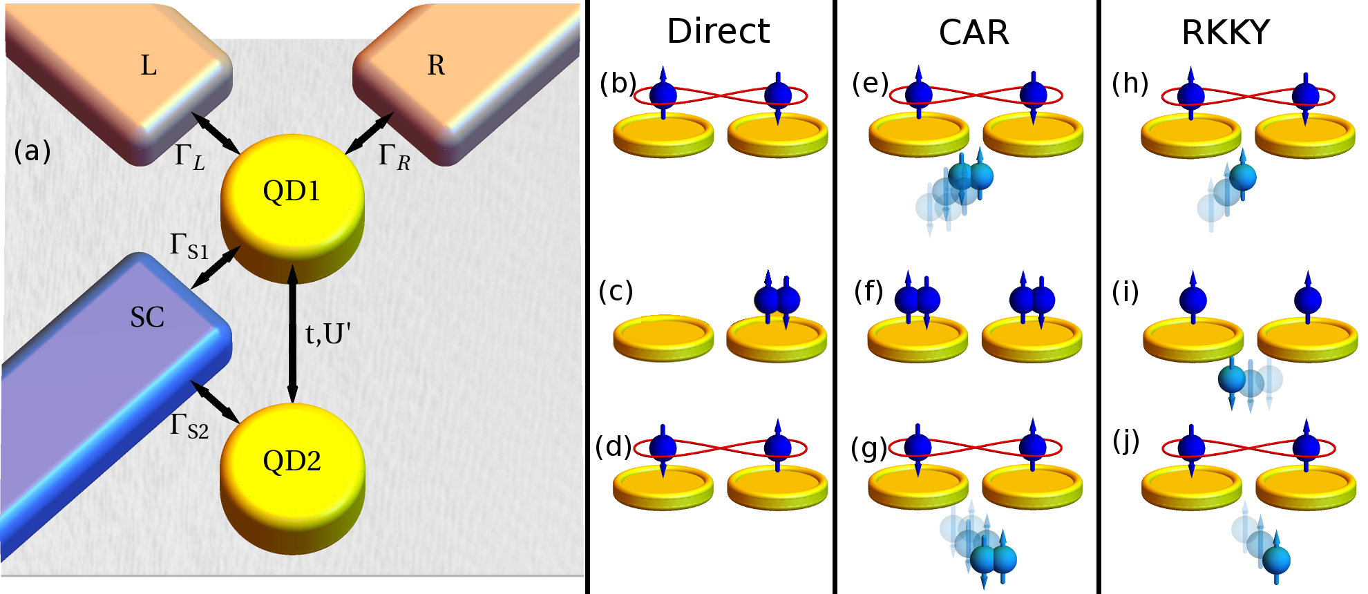
Figure 1: (a) Schematic of the considered system. Left/right (L/R) lead is coupled to the first quantum dot (QD1), while superconductor is attached to both QD1 and QD2. (b)-(d) illustrate an example of direct spin exchange: spin-up electron from the initial state (b) hops to the other QD (c) and spin-down electron hops back (d). Note, that the final state is in fact the same singlet state, only with opposite sign. (e)-(g) show an example of process contributing to crossed Andreev reflection (CAR) exchange. A Cooper pair from SC approaches DQD (e) and two singlets of the same charge are formed (f), before the Cooper pair is re-emitted (g). (h)-(j) present an example of RKKY process: an electron scattered off one QD (h) mediates the spin exchange towards the other (i), before it is finally scattered off there, too (j).

In this paper we discuss the CAR-induced Kondo screening in a setup comprising T-shaped DQD with normal and superconducting contacts, see Fig. 1(a). We note that despite quite generic character of CAR exchange, and its presence in systems containing at least two localized electrons coupled close to each other to the same SC bath, to best of our knowledge CAR-induced screening has hardly been identified in previous studies Hofstetter et al. (2009); Herrmann et al. (2010); Schindele et al. (2012); Das et al. (2012); Borzenets et al. (2016); Wrześniewski and Weymann (2017); Yao et al. (2014b); Žitko et al. (2010); Žitko (2015); Busz et al. (2017). In the system proposed here [Fig. 1(a)], its presence is evident. Moreover, CAR exchange magnitude can be directly related to the relevant energy scales, such as the Kondo temperature, which provides a fingerprint for quantitative experimental verification of our predictions.

The paper is organized as follows. In Sec. II we describe the considered system and present the model we use to study it. In Sec. III the relevant energy scales are estimated to make the discussion of main results concerning CAR-induced Kondo effect in Sec. IV more clear. Finally, the influence of effects neglected in Sec. IV are presented in the following sections, including CAR exchange interplay with RKKY interaction (Sec. V), particle-hole asymmetry (Sec. VI), couplings asymmetry (Sec. VII) and reduced efficiency of CAR coupling (Sec. VIII). In summary, the effects discussed in Sec. IV remain qualitatively valid in all these cases. The paper is concluded in Sec. IX.

II Model

The schematic of the considered system is depicted in Fig. 1(a). It contains two QDs attached to a common SC lead. Only one of them (QD1) is directly attached to the left (L) and right (R) normal leads, while the other dot (QD2) remains coupled only through QD1. The SC is modeled by the BCS Hamiltonian, $H_{\mathrm{S}}=\sum_{\mathbf{k}\sigma}\xi_{\mathbf{k}}a_{\mathbf{k}\sigma}^{{\dagger}}a_{\mathbf{k}\sigma}-\Delta\sum_{\mathbf{k}}(a^{\dagger}_{\mathbf{k}\uparrow}a_{-\mathbf{k}\downarrow}^{{\dagger}}+a_{-\mathbf{k}\downarrow}a_{\mathbf{k}\uparrow})$, with energy dispersion $\xi_{\mathbf{k}}$, energy gap $2\Delta>0$ and $a_{\mathbf{k}\sigma}$ annihilation operator of electron possessing spin $\sigma$ and momentum $\mathbf{k}$. The coupling between SC and QDs is described by the hopping Hamiltonian $H_{\mathrm{TS}}=\sum_{i\mathbf{k}\sigma}v_{\mathrm{S}i}(d^{\dagger}_{i\sigma}a_{\mathbf{k}\sigma}+h.c.)$, with $d^{\dagger}_{i\sigma}$ creating a spin-$\sigma$ electron at QD$i$. The matrix element $v_{\mathrm{S}i}$ and the normalized density of states of SC in normal state, $\rho_{\rm S}$, contribute to the coupling of QD$i$ to SC electrode as $\Gamma_{\mathrm{S}i}=\pi\rho_{\rm S}|v_{{\rm S}i}|^{2}$. We focus on the sub-gap regime, therefore, we integrate out SC degrees of freedom lying outside the energy gap Rozhkov and Arovas (2000). This gives rise to the following effective Hamiltonian, $H_{\mathrm{eff}}=H_{\mathrm{SDQD}}+H_{\rm L}+H_{\rm R}+H_{\rm T}$, where

$$H_{\rm SDQD} = \sum_{i\sigma}\varepsilon_{i}n_{i\sigma}+\sum_{i}Un_{i\uparrow}n_{i\downarrow}+U^{\prime}(n_{1}-1)(n_{2}-1)$$ (1)

$$+ \sum_{\sigma}t(d^{\dagger}_{1\sigma}d_{2\sigma}+h.c.)+J\vec{S}_{1}\vec{S}_{2}$$

$$+ \sum_{i}\!\!\left[\Gamma_{{\rm S}i}(d^{\dagger}_{i\uparrow}d^{\dagger}_{i\downarrow}\!+\!h.c.)+\Gamma_{\rm SX}(d^{\dagger}_{i\uparrow}d^{\dagger}_{\bar{i}\downarrow}\!+\!h.c.)\right]$$

is the Hamiltonian of the SC-proximized DQD Wrześniewski and Weymann (2017); Walldorf et al. (2018), with QD$i$ energy level $\varepsilon_{i}$, inter-site (intra-site) Coulomb interactions $U^{\prime}$ ($U$), inter-dot hopping $t$, and CAR coupling $\Gamma_{\mathrm{S}\rm X}$. $n_{i\sigma}=d^{\dagger}_{i\sigma}d_{i\sigma}$ denotes the electron number operator at QD$i$, $n_{i}=n_{\uparrow}+n_{\downarrow}$, and $\bar{i}\equiv 3-i$. Our model is strictly valid in the regime where $\Delta$ is the largest energy scale. Nevertheless, all discussed phenomena are present in a full model for energies smaller than SC gap. Moreover, by eliminating other consequences of the presence of SC lead, our model pinpoints the fact that the non-local pairing is sufficient for the occurrence of the CAR exchange. The presence of out-gap states shall result mainly in additional broadening of DQD energy levels, changing the relevant Kondo temperatures. We note that the procedure of integrating out out-gap states neglects the RKKY interaction mediated by SC lead and other possible indirect exchange mechanisms. To compensate for this, we explicitly include the Heisenberg term $J\vec{S}_{1}\vec{S}_{2}$ in $H_{\rm SDQD}$, with $\vec{S}_{i}$ denoting the spin operator of QD$i$ and a Heisenberg coupling $J$ substituting the genuine RKKY exchange.

The normal leads are treated as reservoirs of noninteracting electrons, $H_{r}=\sum_{\mathbf{k}\sigma}\varepsilon_{r\mathbf{k}}c^{\dagger}_{r\mathbf{k}\sigma}c_{r\mathbf{k}\sigma}$, where $c_{r\mathbf{k}\sigma}$ annihilates an electron of spin $\sigma$ and momentum $\mathbf{k}$ in lead $r$ ($r={\rm L,R}$) with the corresponding energy $\varepsilon_{r\mathbf{k}\sigma}$. The tunneling Hamiltonian reads, $H_{\rm T}=\sum_{r\mathbf{k}\sigma}v_{r}(d^{\dagger}_{1\sigma}c_{r\mathbf{k}\sigma}+h.c.)$, giving rise to coupling between lead $r$ and QD$i$ of strength $\Gamma_{r}=\pi\rho_{r}|v_{r}|^{2}$, with $\rho_{r}$ the normalized density of states of lead $r$ and $v_{r}$ the local hopping matrix element, assumed momentum-independent. We consider a wide-band limit, assuming constant $\Gamma_{r}=\Gamma/2$ within the cutoff $\pm D=\pm 2U$ around the Fermi level.

For thorough analysis of the CAR exchange mechanism and its consequences for transport, we determine the linear conductance between the two normal leads from

$$G=\frac{2e^{2}}{h}\pi\Gamma\int\left[-\frac{\partial f_{T}}{\partial\omega}\right]\mathcal{A}(\omega){\rm d}\omega,$$ (2)

where $f_{T}$ is the Fermi function at temperature $T$, while $\mathcal{A}(\omega)$ denotes the normalized local spectral density of QD1 fn (1). Henceforth, unless we state otherwise, we assume a maximal CAR coupling, $\Gamma_{\mathrm{S}\rm X}=\sqrt{\Gamma_{\mathrm{S}1}\Gamma_{\mathrm{S}2}}$ Wrześniewski and Weymann (2017); Walldorf et al. (2018), $\Gamma_{\mathrm{S}1}=\Gamma_{\mathrm{S}2}=\Gamma_{\mathrm{S}}$ and consider DQD tuned to the particle-hole symmetry point, $\varepsilon_{1}=\varepsilon_{2}=-U/2$. However, these assumptions are not crucial for the results presented here, as discussed in Secs. VI-VIII.

III Estimation of relevant energy scales

Since we analyze a relatively complex system, let us build up the understanding of its behavior starting from the case of a QD between two normal-metallic leads, which can be obtained in our model by setting $t=\Gamma_{\mathrm{S}}=J=U^{\prime}=0$. Then, the conductance as a function of temperature, $G(T)$, grows below the Kondo temperature $T_{K}$ and reaches maximum for $T\to 0$, $G(T\!=\!0)=G_{\rm max}$. At particle-hole symmetry point, the unitary transmission is achieved, $G_{\rm max}=G_{0}=2e^{2}/h$; see short-dashed line in Fig. 2(a). An experimentally relevant definition of $T_{K}$ is that at $T=T_{K}$ $G(T)=G_{\rm max}/2$. $T_{K}$ is exponentially small in the local exchange $J_{0}=8\Gamma/(\pi\rho U)$, and is approximated by $T_{K}\approx D\exp[-1/(\rho J_{0})]$ Hewson (1997).

The presence of a second side-coupled QD, $t,U^{\prime}>0$, significantly enriches the physics of the system by introducing direct exchange between QDs, see Fig. 1(b-d). In general, effective inter-dot exchange can be defined as energy difference between the triplet and singlet states of isolated DQD, $J^{\mathrm{eff}}=E_{S=1}-E_{\rm GS}$. Unless $U$ becomes very large, superexchange can be neglected Lee et al. (2010) and $J^{\mathrm{eff}}$ is determined by direct exchange, $J^{\mathrm{eff}}\approx 4t^{2}/(U-U^{\prime})>0$. When the hopping $t$ is tuned small Hofstetter et al. (2009), one can expect $J^{\mathrm{eff}}\lesssim T_{K}$, which implies the two-stage Kondo screening Pustilnik and Glazman (2001); Cornaglia and Grempel (2005). Then, for $T\ll T_{K}$, the local spectral density of QD1 serves as a band of width $\sim T_{K}$ for QD2. The spin of an electron occupying QD2 experiences the Kondo screening below the associated Kondo temperature

$$T^{*}=aT_{K}\exp(-bT_{K}/J_{\rm eff})$$ (3)

with $a$ and $b$ constants of order of unity Pustilnik and Glazman (2001); Cornaglia and Grempel (2005). This is reflected in conductance, which drops to $0$ with lowering $T$, maintaining characteristic Fermi-liquid $G\sim T^{2}$ dependence Cornaglia and Grempel (2005); see the curves indicated with squares in Fig. 2(a). Similarly to $T_{K}$, experimentally relevant definition of $T^{*}$ is that $G(T\!=\!T^{*})=G_{\rm max}/2$. Even at the particle-hole symmetry point $G_{\rm max}<G_{0}$, because the single-QD strong-coupling fixed point is unstable in the presence of QD2 and $G(T)$ does not achieve $G_{0}$ exactly, before it starts to decrease.

The proximity of SC gives rise to two further exchange mechanisms that determine the system’s behavior. First of all, the (conventional) RKKY interaction appears, $J\sim\Gamma_{\mathrm{S}}^{2}$ Ruderman and Kittel (1954); Kasuya (1956); Yosida (1957). Moreover, the CAR exchange emerges as a consequence of finite $\Gamma_{\mathrm{S}}$ Yao et al. (2014a). It can be understood on the basis of perturbation theory as follows. DQD in the inter-dot singlet state may absorb and re-emit a Cooper pair approaching from SC; see Fig. 1(e)-(g). As a second-order process, it reduces the energy of the singlet, which is the ground state of isolated DQD. A similar process is not possible in the triplet state due to spin conservation. Therefore, the singlet-triplet energy splitting $J^{\mathrm{eff}}$ is increased (or generated for $t=J=0$). More precisely, the leading ($2$nd-order in $t$ and $\Gamma_{\mathrm{S}}$) terms in the total exchange are

$$J^{\mathrm{eff}}\approx J+\frac{4t^{2}}{U-U^{\prime}+\frac{3}{4}J}+\frac{4\Gamma_{\mathrm{S}}^{2}}{U+U^{\prime}+\frac{3}{4}J}.$$ (4)

Using this estimation, one can predict $T^{*}$ for finite $\Gamma_{\mathrm{S}}$, $t$ and $J$ with Eq. (3). Apparently, from three contributions corresponding to: (i) RKKY interaction, (ii) direct exchange and (iii) CAR exchange, only the first may bear a negative (ferromagnetic) sign. The two other contributions always have an anti-ferromagnetic nature. More accurate expression for $J^{\mathrm{eff}}$ is derived in Appendix A [see Eq. (13)] by the Hamiltonian down-folding procedure. The relevant terms differ by factors important only for large $\Gamma_{\mathrm{S}}/U$. Finally, it seems worth stressing that normal leads are not necessary for CAR exchange to occur. At least one of them is inevitable for the Kondo screening though, and two symmetrically coupled normal leads allow for measurement of the normal conductance.

It is also noteworthy that inter-dot Coulomb interactions decrease the energy of intermediate states contributing to direct exchange [Fig. 1(c)], while increasing the energy of intermediate states causing the CAR exchange [Fig. 1(f)]. This results in different dependence of corresponding terms in Eq. (4) on $U^{\prime}$. As can be seen in Figs. 2(b) and 2(c), it has a significant effect on the actual values of $T^{*}$.

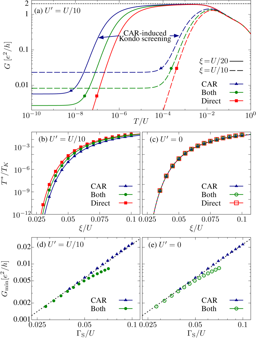
Figure 2: (a) Linear conductance $G$ as function of $T$ calculated for $\varepsilon_{1}=\varepsilon_{2}=-U/2$, $\Gamma=U/5$, $U^{\prime}=U/10$ and different situations, as indicated. The quantity $\xi\equiv\sqrt{\Gamma_{\mathrm{S}}^{2}+t^{2}}$ is fixed for different curves drawn with the same dashing style. Note the logarithmic scale on both axes. (b) Points show $T^{*}/T_{K}$ calculated by NRG from curves in subfigure (a). Lines present the fit to Eq. (3) with $J^{\mathrm{eff}}$ obtained from Eq. (4). (c) The same as (b), only for $U^{\prime}=0$. (d) and (e) show the residual conductance $G_{\mathrm{min}}\equiv G(T\!=\!0)$ as a function of $\Gamma_{\mathrm{S}}$ for $t=0$ (denoted ”CAR”) and $t=\Gamma_{\mathrm{S}}$ (denoted ”Both”). Dotted line is a guide for eyes. $U^{\prime}=U/10$ in (b) and (d) and $U^{\prime}=0$ in (c) and (e).

IV CAR exchange and Kondo effect

To verify Eqs. (3)-(4) we calculate $G$ using accurate full density matrix numerical renormalization group (NRG) technique Wilson (1975); Weichselbaum and von Delft (2007); Fle ; fn (2). We compare $U^{\prime}=0$ case with experimentally relevant value $U^{\prime}=U/10$ Keller et al. (2013). While for two close adatoms on SC surface RKKY interactions may lead to prominent consequences Klinovaja et al. (2013), the conventional (i.e. non-CAR) contribution should vanish rapidly when the inter-impurity distance $r$ exceeds a few lattice constants Mitchell et al. (2015); Bulaevskii et al. (1985). Meanwhile, the CAR exchange may remain significant for $r$ of the order of coherence length of the SC contact Yao et al. (2014a). Therefore, we first neglect the conventional RKKY coupling and analyze its consequences in Sec. V.

The main results are presented in Fig. 2(a), showing the temperature dependence of $G$ for different circumstances. For reference, results for $\Gamma_{\mathrm{S}}=0$ are shown, exhibiting the two-stage Kondo effect caused by direct exchange mechanism. As can be seen in Figs. 2(b) and 2(c), an excellent agreement of $T^{*}$ found from NRG calculations and Eq. (3) is obtained with $a=0.42$ and $b=1.51$, the same for both $U^{\prime}=0$ and $U^{\prime}=U/10$. Note, however, that $J^{\mathrm{eff}}$ is different in these cases, cf. Eq. (4), and $U^{\prime}$ leads to increase of $T^{*}$.

Furthermore, for $t=0$ and $\Gamma_{\mathrm{S}}>0$ the two-stage Kondo effect caused solely by the CAR exchange is present; see Fig. 2(a). Experimentally, this situation corresponds to a distance between the two QDs smaller than the superconducting coherence length, but large enough for the exponentially suppressed direct hopping to be negligible. While intuitively one could expect pairing to compete with any kind of magnetic ordering, the Kondo screening induced by CAR exchange is a beautiful example of a superconductivity in fact leading to magnetic order, namely the formation of the Kondo singlet. This CAR-exchange-mediated Kondo screening is our main finding. For such screening, Eq. (3) is still fulfilled with very similar parameters, $a=0.37$ ($a=0.35$) and $b=1.51$ ($b=1.50$) for $U^{\prime}=0$ ($U^{\prime}=U/10$), correspondingly; see Figs. 2(b-c). Moreover, as follows from Eq. (4), $U^{\prime}$ reduces CAR exchange, and therefore diminishes $T^{*}$. For the same values of $J^{\mathrm{eff}}$, the dependence of $G(T)$ for $t=0$ and $\Gamma_{\mathrm{S}}>0$ is hardly different from the one for $\Gamma_{\mathrm{S}}=0$ and $t>0$ for $T\geq T^{*}$ (results not shown). However, $G(T)$ saturates at residual value $G_{\mathrm{min}}$ as $T\to 0$ only for finite $\Gamma_{\mathrm{S}}$, which at particle-hole symmetry makes $G_{\mathrm{min}}$ the hallmark of SC proximity and the corresponding CAR exchange processes. From numerical results, one can estimate it as

$$G_{\mathrm{min}}=\frac{e^{2}}{h}\cdot c\,\frac{\Gamma_{\mathrm{S}}^{2}}{U^{2}}\qquad{\scriptstyle(\Gamma_{\mathrm{S}1}=\Gamma_{\mathrm{S}2}=\Gamma_{\mathrm{S}})},$$ (5)

with $c\approx 2.25$, barely depending on $U^{\prime}$ and getting smaller for $t>0$. This is illustrated in Figs. 2(d-e), where the dotted line corresponds to Eq. (5) with $c=2.25$.

Lastly, in Fig. 2(a) we also present the curves obtained for $t=\Gamma_{\mathrm{S}}$ chosen such, that the quantity $\xi=\sqrt{t^{2}+\Gamma_{\mathrm{S}}^{2}}$ remains the same in all the cases. This is to illustrate what happens when both (direct and CAR) exchange interactions are present. Fig. 2(c) clearly shows that $T^{*}$ remains practically unaltered for $U^{\prime}=0$. The comparison with Fig. 2(b) proves that in this case it practically does not depend on $U^{\prime}$. The enhancement of direct exchange is compensated by the decrease of the CAR one. On the contrary, $G_{\mathrm{min}}$ decreases for larger $t$ below the estimation given by Eq. (5), as can be seen in Figs. 2(d-e).

While analyzing the results concerning $G_{\mathrm{min}}(\Gamma_{\mathrm{S}})$ plotted in Figs. 2(d-e) one needs to keep in mind that $G_{\mathrm{min}}$ is obtained at deeply cryogenic conditions. To illustrate this better, $G(\Gamma_{\mathrm{S}})$ obtained for $t=0$ and $T=10^{-6}U$ is plotted with solid line in Fig. 3. Clearly, for weak $\Gamma_{\mathrm{S}}$ the system exhibits rather conventional (single-stage) Kondo effect with $G=G_{\mathrm{max}}\approx 2e^{2}/h$, while QD2 is effectively decoupled ($G_{\mathrm{max}}<2e^{2}/h$ in the proximity of SC lead Wójcik and Weymann (2014)). Only for larger values of $\Gamma_{\mathrm{S}}$ the CAR exchange is strong enough, such that $T^{*}>T$ and the dependence $G(\Gamma_{\mathrm{S}})$ continuously approaches the $T=0$ limit estimated by Eq. (5) and presented in Figs. 2(d-e).

V CAR-RKKY competition

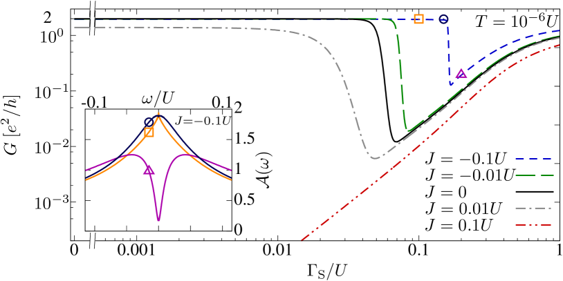
Figure 3: Linear conductance $G$ vs. $\Gamma_{\mathrm{S}}$ calculated for $t=0$, $\Gamma=U/5$, $U^{\prime}=U/10$, finite $T=10^{-6}U$ and different values of RKKY coupling $J$, as indicated. Inset shows QD1 spectral function $\mathcal{A}(\omega)$ as a function of energy $\omega$ for points on $J=-0.1U$ curve, indicated with corresponding symbols.

Let us now discuss the effects introduced by the conventional RKKY interaction. We choose $t=0$ for the sake of simplicity and analyze a wide range of $\Gamma_{\mathrm{S}}$, starting from the case of anti-ferromagnetic RKKY interaction ($J>0$). Large $J>0$ leads to the formation of a molecular singlet in the nanostructure. This suppresses the conductance, unless $\Gamma_{\mathrm{S}}$ becomes of the order of $U/2$, when the excited states of DQD are all close to the ground state. This is illustrated by double-dotted line in Fig. 3. Smaller value of $J>0$ causes less dramatic consequences, namely it just increases $J^{\mathrm{eff}}$ according to Eq. (4), leading to enhancement of $T^{*}$, cf. Eq. (3). This is presented with dot-dashed line in Fig. 3.

The situation changes qualitatively for ferromagnetic RKKY coupling, $J<0$. Then, RKKY exchange and CAR exchange have opposite signs and compete with each other. Depending on their magnitudes and temperature, one of the following scenarios may happen.

For $J^{\mathrm{eff}}>0$, i.e. large enough $\Gamma_{\mathrm{S}}$, and $T<T^{*}$, the system is in the singlet state due to the two-stage Kondo screening of DQD spins. $G(T\!=\!0)$ is reduced to $G_{\mathrm{min}}$, which tends to increase for large negative $J$; see dashed lines in Fig. 3. In the inset to Fig. 3, the spectral density of QD1 representative for this regime is plotted as curve indicated by triangle. It corresponds to a point on the $J=-0.1U$ curve in the main plot, also indicated by triangle. The dip in $\mathcal{A}(\omega)$ has width of order of $T^{*}$.

For finite $T$, there is always a range of sufficiently small $|J^{\mathrm{eff}}|$, where QD2 becomes effectively decoupled, and, provided $T<T_{K}$, $G$ reaches $G_{\mathrm{max}}$ due to conventional Kondo effect at QD1. This is the case for sufficiently small $\Gamma_{\mathrm{S}}$ for $J=0$ or $J=-0.01U$, and in the narrow range of $\Gamma_{\mathrm{S}}$ around the point indicated by a circle in Fig. 3 for $J=-0.1U$ (for $J=0.01U$, the considered $T$ is close to $T^{*}$ and $G$ does not reach $G_{\rm max}$). The conventional Kondo effect manifests itself with a characteristic peak in $\mathcal{A}(\omega)$, as illustrated in the inset in Fig. 3 with line denoted by circle.

Finally, large enough $J^{\mathrm{eff}}<0$ and low $T$, give rise to an effective ferromagnetic coupling of DQDs spins into triplet state. Consequently, the underscreened Kondo effect occurs Mattis (1967); Nozières and Blandin (1980) for weak $\Gamma_{\mathrm{S}}$ and, e.g., $J=-0.1U$; see the point indicated by square in Fig. 3. This leads to $G=G_{\mathrm{max}}$ and a peak in $\mathcal{A}(\omega)$, whose shape is significantly different from the Kondo peak, cf. the curve denoted by square in the inset in Fig. 3.

VI Effects of detuning from the particle-hole symmetry point

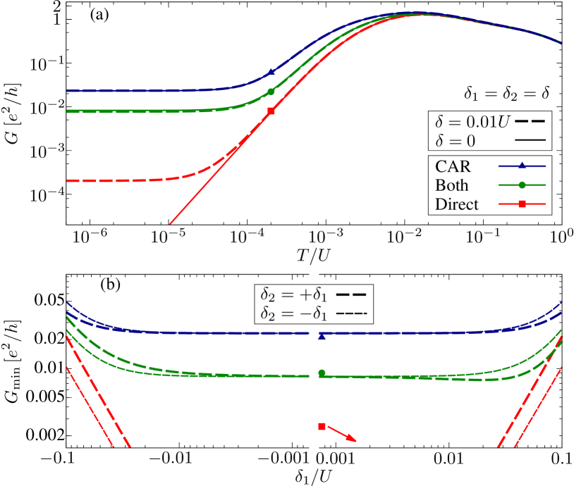
Figure 4: (a) Linear conductance between the normal leads $G$ as a function of temperature $T$ for parameters corresponding to Fig. 2(a) with $\xi=U/10$, and additional curves for finite detuning from particle-hole symmetry point, $\delta_{1}=-\delta_{2}$, and two values of $\xi=\sqrt{t^{2}+\Gamma_{\mathrm{S}}^{2}}$, as indicated in the figure. (b) $G_{\mathrm{min}}\equiv G(T\!=\!0)$ as a function of QD1 detuning $\delta_{1}$ for different exchange mechanisms, $\xi=U/10$ and $\delta_{2}=\pm\delta_{1}$ (as indicated).

At PHS $G_{\mathrm{min}}=G(T\!=\!0)=0$ in the absence of superconducting lead, making $G_{\mathrm{min}}>0$ a hallmark of SC-induced two-stage Kondo effect. However, outside of PHS point $G_{\mathrm{min}}>0$ even in the case of the two-stage Kondo effect caused by the direct exchange. Exact PHS conditions are hardly possible in real systems, and the fine-tuning of the QD energy levels to PHS point is limited to some finite accuracy. Therefore, there may appear a question, if the results obtained at PHS are of any importance for the realistic setups. As we show below — they are, in a reasonable range of detunings $\delta_{i}=\varepsilon_{i}+U/2$.

In Fig. 4(a) we present the $G(T)$ dependence in and outside the PHS, corresponding to parameters of Fig. 2(a). Clearly, for considered small values of $\delta_{1}=\delta_{2}=\delta$, $G_{\mathrm{min}}<10^{-3}e^{2}/h$ for direct exchange only, while $G_{\mathrm{min}}$ in the presence of a superconductor is significantly increased and close to the PHS value. Furthermore, for $|\delta_{1}|\sim|\delta_{2}|\sim\delta$, the residual conductance caused by the lack of PHS, $G_{\mathrm{min}}\approx e^{2}/h\cdot(\delta/U)^{2}$, which is a rapidly decreasing function in the vicinity of PHS point, as illustrated in Fig. 4(b) with lines denoted by a square. Evidently, in the regime $|\delta_{i}|<0.01U$ the residual conductance caused by SC is orders of magnitude larger, leading to the plateau in $G_{\mathrm{min}}(\delta_{1})$ dependence, visible in Fig. 4(b). Taking into account that the realistic values of $U$ in the semiconductor quantum dots are rather large, this condition seems to be realizable by fine-tuning of QD gate voltages.

Lastly, let us point out that while in the presence of only one exchange mechanism, CAR or direct, $G_{\mathrm{min}}(\delta_{1})$ dependencies depicted in Fig. 4(b) are symmetrical with respect to sign change of $\delta_{1}$, for both exchange mechanisms the dependence is non-symmetric.

VII Effects of asymmetry of couplings to superconductor

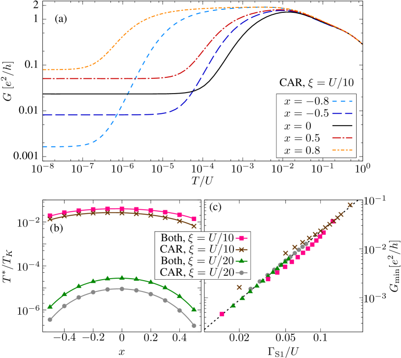
Figure 5: (a) Linear conductance between the normal leads, $G$, as a function of temperature, $T$, for parameters corresponding to Fig. 2(a) with $\xi=U/10$, for different values of asymmetry coefficient $x$ [see Eq. (6)], in the presence of CAR exchange only. (b) The second-stage Kondo temperature $T^{*}$ normalized by $T_{K}$ as a function of $x$, calculated with the aid of NRG (points) and a fit to Eq. (3) (lines) with $J^{\mathrm{eff}}$ from Eq. (4). (c) The zero-temperature conductance $G_{\mathrm{min}}$ as a function of QD1 coupling to SC lead, $\Gamma_{\mathrm{S}1}$, compiled from data obtained at different circumstances (as indicated in the legend) for different $x$. Dotted line corresponds to Eq. (8) with $c=2.25$.

Similarly to PHS, the ideal symmetry in the coupling between respective QDs and SC lead is hardly possible in experimental reality. As shown below, it does not introduce any qualitatively new features. On the other hand, it decreases the second stage Kondo temperature, which is already small, therefore, quantitative estimation of this decrease may be important for potential experimental approaches. To analyze the effects of $\Gamma_{\mathrm{S}1}\neq\Gamma_{\mathrm{S}2}$, we introduce the asymmetry parameter $x$ and extend the definition of $\Gamma_{\mathrm{S}}$,

$$x=\frac{\Gamma_{\mathrm{S}1}-\Gamma_{\mathrm{S}2}}{\Gamma_{\mathrm{S}1}+\Gamma_{\mathrm{S}2}},\quad\Gamma_{\mathrm{S}}=\frac{\Gamma_{\mathrm{S}1}+\Gamma_{\mathrm{S}2}}{2}.$$ (6)

Note, that even for a fixed $\Gamma_{\mathrm{S}}$, the actual CAR coupling $\Gamma_{\mathrm{S}\rm X}=\Gamma_{\mathrm{S}}\sqrt{1-x^{2}}$ decreases with increasing $|x|$, which is a main mechanism leading to a decrease of $T^{*}$ outside the $x=0$ point visible in Figs. 5(a) and (b). To illustrate this, the curves corresponding to both exchange mechanisms were calculated using $x$-dependent $t=\Gamma_{\mathrm{S}\rm X}$ instead of $t=\xi/\sqrt{2}$. Therefore, $\xi$ was generalized for $x\neq 0$ by setting $\xi=\sqrt{t^{2}(1-x^{2})^{-1}+\Gamma_{\mathrm{S}}^{2}}$. Clearly, in Fig. 5(b) the curves for different exchange mechanisms are very similar and differ mainly by a constant factor, resulting from different influence of $U^{\prime}$; see Sec. III. The magnitude of $T^{*}$ changes is quite large, exceeding an order of magnitude for $x=\pm 0.5$ and $\xi=U/20$. Moreover, $T^{*}\to 0$ for $x\to\pm 1$. Consequently, for strongly asymmetric devices one cannot hope to observe the second stage of Kondo screening.

A careful observer can note that the $T^{*}(x)$ dependency is not symmetrical; note for example different $T^{*}$ for $x=\pm 0.5$ in Fig. 5(a). This is caused by the dependence of the first stage Kondo temperature $T_{K}$ on $\Gamma_{\mathrm{S}1}$ Wójcik and Weymann (2018); Domański et al. (2016),

$$\widetilde{T}_{K}(\Gamma_{\mathrm{S}1})=T_{K}\cdot\exp\!\left(\frac{\pi}{2}\frac{\Gamma_{\mathrm{S}1}^{2}}{\Gamma U}\right).$$ (7)

Here, $T_{K}$ is, as earlier, defined in the absence of SC, while $\widetilde{T}_{K}$ is a function of $\Gamma_{\mathrm{S}1}$, such that $G(\widetilde{T}_{K})=G_{\rm max}(\Gamma_{\mathrm{S}1})/2$ in the absence of QD2. As $\widetilde{T}_{K}$ grows for increasing $\Gamma_{\mathrm{S}1}$ (or $x$), $T^{*}$ decreases according to Eq. (3). Its $\Gamma_{\mathrm{S}}$ dependence can be accounted for by small changes in the coefficients $a$ and $b$ in Eq. (3), as long as $x$ is kept constant.

To close the discussion of $T^{*}(x)$ dependence let us point out, that in Eq. (13) there appears a correction to Eq. (4) for $x\neq 0$. However, it is very small due to additional factor $\Gamma_{\mathrm{S}}^{2}/U^{2}$ in the leading order. Its influence on curves plotted in Fig. 5(b) is hardly visible.

In turn, let us examine the $x$ dependence of the $T=0$ conductance $G_{\mathrm{min}}$. As can be seen in Fig. 5(a), it monotonically increases with $x$, as it crosses $x=0$ point. In fact, Eq. (5) can be generalized to

$$G_{\mathrm{min}}=\frac{e^{2}}{h}\cdot c\,\frac{\Gamma_{\mathrm{S}1}^{2}}{U^{2}},$$ (8)

with $c\approx 2.25$ (indicated by a dotted line in Fig. 5(c)). Note that $G_{\mathrm{min}}$ is proportional to $\Gamma_{\mathrm{S}1}^{2}=(x+1)^{2}\Gamma_{\mathrm{S}}^{2}$, instead of simply $\Gamma_{\mathrm{S}}$, cf. Eq. (5). The values of $G_{\mathrm{min}}$ obtained from all analyzed $G(T)$ dependencies for different $x$ have been compiled in Fig. 5(c). It is evident, that Eq. (8) is approximately fulfilled for all the considered cases.

Finally, it seems noteworthy that the normal-lead coupling asymmetry, $\Gamma_{\rm L}\neq\Gamma_{\rm R}$, is irrelevant for the results except for a constant factor diminishing the conductance $G$ Wójcik et al. (2013).

VIII The role of CAR efficiency

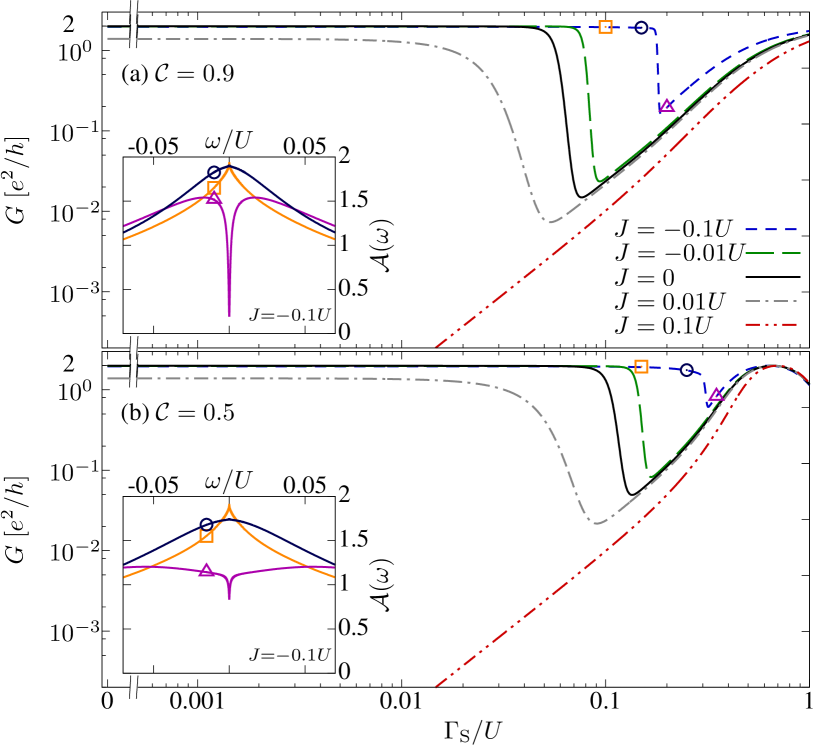
Figure 6: Linear conductance between the normal leads $G$ as a function of coupling to SC lead, $\Gamma_{\mathrm{S}}$, for indicated values of RKKY exchange $J$ and the efficiency of CAR processes reduced by factor (a) $\mathcal{C}=0.9$ and (b) $\mathcal{C}=0.5$. Other parameters as in Fig. 3. Insets: QD1 local spectral density $\mathcal{A}(\omega)$ as a function of energy $\omega$ for points on $J=-0.1U$ curve, indicated with corresponding symbols.

Up to this point we assumed $\Gamma_{\mathrm{S}\rm X}=\sqrt{\Gamma_{\mathrm{S}1}\Gamma_{\mathrm{S}2}}$, which is valid when the two quantum dots are much closer to each other than the coherence length in the superconductor. This does not have to be the case in real setups, yet relaxing this assumption does not introduce qualitative changes. Nevertheless, the model cannot be extended to inter-dot distances much larger than the coherence length, where $\Gamma_{\mathrm{S}\rm X}\to 0$.

To quantitatively analyze the consequences of less effective Andreev coupling we define the CAR efficiency as $\mathcal{C}\equiv\Gamma_{\mathrm{S}\rm X}/\sqrt{\Gamma_{\mathrm{S}1}\Gamma_{\mathrm{S}2}}$ and analyze $\mathcal{C}<1$ in the wide range of $\Gamma_{\mathrm{S}1}=\Gamma_{\mathrm{S}2}=\Gamma_{\mathrm{S}}$ and other parameters corresponding to Fig. 3. The results are presented in Fig. 6.

Clearly, decreasing $\mathcal{C}$ from $\mathcal{C}=1$ causes diminishing of $\Gamma_{\mathrm{S}\rm X}$, and consequently of CAR exchange. For a change as small as $\mathcal{C}=0.9$, the consequences reduce to some shift of the conventional Kondo regime, compare Fig. 6(a) with Fig. 3. Stronger suppression of CAR may, however, increase the SC coupling necessary to observe the second stage of Kondo screening caused by CAR outside the experimentally achievable range, see Fig. 6(b). Moreover, the reduced $T^{*}$ leads to narrowing of the related local spectral density dip, while the increased critical $\Gamma_{\mathrm{S}}$ necessary for the observation of the second stage of screening leads to the shallowing of the dip. This is visible especially in the inset in Fig. 6(b).

IX Conclusions

The CAR exchange mechanism is present in any system comprising at least two QDs or magnetic impurities coupled to the same superconducting contact in a way allowing for crossed Andreev reflections. In the considered setup, comprised of two quantum dots in a T-shaped geometry with respect to normal leads and proximized by superconductor, it leads to the two-stage Kondo screening even in the absence of other exchange mechanisms. This CAR induced exchange screening is characterized by a residual low-temperature conductance at particle-hole symmetric case. We have also shown that the competition between CAR exchange and RKKY interaction may result in completely different Kondo screening scenarios.

The presented results bring further insight into the low-temperature behavior of hybrid coupled quantum dot systems, which hopefully could be verified with the present-day experimental techniques. Moreover, non-local pairing is present also in bulk systems such as non-$s$-wave superconductors. The question if an analogue of discussed CAR exchange may play a role there seems intriguing in the context of tendencies of many strongly correlated materials to possess superconducting and anti-ferromagnetic phases.

Appendix A More precise estimation of the effective exchange

We first briefly describe the Hamiltonian down-folding method, then we apply it to the model considered in the main paper.

A.1 General formulation of down-folding method

Say we have the full Hilbert space of states divided into two sections, A and B. We think of A as being most important and of B as some addition, typically a set of high-energy states (in terms of the non-interacting part of the Hamiltonian). We can structure the secular equation for $H$ as follows,

$$\left[\begin{array}[]{cc}H_{\rm A}&H_{\rm AB}^{\dagger}\\ H_{\rm AB}&H_{\rm B}\end{array}\right]\left[\begin{array}[]{c}\psi_{\rm A}\\ \psi_{\rm B}\end{array}\right]=E\left[\begin{array}[]{c}\psi_{\rm A}\\ \psi_{\rm B}\end{array}\right].$$ (9)

Treating it as a set of linear equations one can calculate components $\psi_{\rm B}$ as functions of matrix elements of $H$, elements of $\psi_{\rm A}$ and the unknown eigenvalue $E$, $\psi_{\rm B}=(E-H_{\rm B})^{-1}H_{\rm AB}\psi_{\rm A}$. Thus, we obtain the equation

$$\left[H_{\rm A}+H_{\rm AB}^{\dagger}(E-H_{\rm B})^{-1}H_{\rm AB}\right]\psi_{\rm A}=E\psi_{\rm A},$$ (10)

where the term in the square bracket can be called the effective Hamiltonian of the states A, $H_{\rm A}^{\rm eff}(E)$. Note, that as long as $E$ on the left-hand-side is not approximated, this expression is exact, nonlinear equation for eigenvalues $E$ of the original, full Hamiltonian and the projections of the full eigenstates $(\psi_{\rm A}\,\psi_{\rm B})^{\rm T}$ onto the space A. In particular, if part A has a finite basis, one obtains the characteristic equation for $H$ eigenvalues by subsequently eliminating one state after another. In practice, however, one is usually interested in eliminating states of high energies and determination of low-energy spectrum of the Hamiltonian, $E\ll H_{\rm B}$. Then, one can put $E\approx 0$. In more general case, $E\approx\langle H_{\rm A}\rangle$ can be used, where $\langle H_{\rm A}\rangle$ is some kind of estimation of the relevant energy. The procedure is valid, as long as the energy dependence of $H_{\rm A}^{\rm eff}(E)$ does not influence its spectrum strongly, in particular for small interaction $H_{\rm AB}$.

A.2 Application to the model under consideration

The spin singlet $S=0$ subspace of the effective Hamiltonian for the superconductor-proximized double quantum dot $H_{\rm SDQD}$ can be written in the form

$$H_{\rm SDQD}^{S=0}=\left[\begin{array}[]{ccccc}-U-\frac{3}{4}J+\delta_{1}+\delta_{2}&t\sqrt{2}&t\sqrt{2}&\Gamma_{\mathrm{S}\rm X}\sqrt{2}&-\Gamma_{\mathrm{S}\rm X}\sqrt{2}\\ t\sqrt{2}&2\delta_{1}-U^{\prime}&0&\Gamma_{\mathrm{S}1}&\Gamma_{\mathrm{S}2}\\ t\sqrt{2}&0&2\delta_{2}-U^{\prime}&\Gamma_{\mathrm{S}2}&\Gamma_{\mathrm{S}1}\\ \Gamma_{\mathrm{S}\rm X}\sqrt{2}&\Gamma_{\mathrm{S}1}&\Gamma_{\mathrm{S}2}&U^{\prime}&0\\ -\Gamma_{\mathrm{S}\rm X}\sqrt{2}&\Gamma_{\mathrm{S}2}&\Gamma_{\mathrm{S}1}&0&2(\delta_{1}+\delta_{2})+U^{\prime}\end{array}\right],$$ (11)

with $\delta_{i}=\varepsilon_{i}+U/2$; see Eq. (1). The order of basis states is as follows: $\left|{1}\right\rangle=2^{-1/2}(\left|{\uparrow\downarrow}\right\rangle-\left|{\downarrow\uparrow}\right\rangle)$, $\left|{2}\right\rangle=\left|{20}\right\rangle$, $\left|{3}\right\rangle=\left|{02}\right\rangle$, $\left|{4}\right\rangle=\left|{00}\right\rangle$, $\left|{5}\right\rangle=\left|{22}\right\rangle$, where $\left|{\chi_{1}\chi_{2}}\right\rangle$ denotes such state, that QD$i$ is in a state $\left|{\chi_{i}}\right\rangle$, and the possible states are $\chi_{i}=0$ (empty QD), $\chi_{i}=2$ (doubly occupied QD), or $\chi_{i}=\sigma$ (QD occupied by a single electron of spin $\sigma$; $\sigma=\uparrow$ or $\sigma=\downarrow$).

From Eq. (11) one can clearly see that in the regime of $U$ dominating over other energy scales there is one state possessing energy of the order of $-U$, and other states have energies regular in the limit $U\to\infty$. Therefore, the first approximation to $E_{\rm GS}$ is the energy of that state, $E_{\rm GS}^{0}=-U-\frac{3}{4}J+\delta_{1}+\delta_{2}$. The down-folding procedure shall be used to correct this estimation. This correction is crucial, since otherwise we get an obvious yet crude result $J^{\mathrm{eff}}=J$.

Let us first examine $\Gamma_{\mathrm{S}1}=\Gamma_{\mathrm{S}2}=\Gamma_{\mathrm{S}\rm X}=\Gamma_{\mathrm{S}}=0$ case. Then, the charge is conserved, so the states $\left|{4}\right\rangle$ and $\left|{5}\right\rangle$ are decoupled. Taking $\left|{1}\right\rangle$ to subspace A, while keeping $\left|{2}\right\rangle$ and $\left|{3}\right\rangle$ in subspace B one gets the estimation of $E_{\rm GS}$, which for $E$ substituted by $E_{\rm GS}^{0}$ leads to

$$J^{\mathrm{eff}}_{\Gamma_{\mathrm{S}}=0}=J+4\frac{t^{2}}{U-U^{\prime}}\left[1-\frac{(\delta_{1}-\delta_{2})^{2}}{(U-U^{\prime})^{2}}\right]^{-1},$$ (12)

in agreement with Refs. Cornaglia and Grempel (2005); Ferreira et al. (2011).

For finite $\Gamma_{\mathrm{S}1}$, $\Gamma_{\mathrm{S}2}$ and $\Gamma_{\mathrm{S}\rm X}$ the situation is more complicated, because there are four states to be eliminated. We assign them all to subspace B and obtain cumbersome expressions, resulting from inverting explicitly non-diagonal $4\times 4$ matrix. Therefore, we limit ourselves to the case of particle-hole symmetry, $\delta_{1}=\delta_{2}=0$. Then, keeping only $\left|{1}\right\rangle$ in subspace A and the remaining $4$ states in B, and using $E\mapsto E_{\rm GS}^{0}$ substitution one gets feasible result,

$$J^{\mathrm{eff}} = J+\frac{4\Gamma_{\mathrm{S}\rm X}^{2}}{U+U^{\prime}+\frac{3}{4}J}\left[1-\frac{4x^{2}\Gamma_{\mathrm{S}}^{2}}{(U+\frac{3}{4}J)^{2}-U^{\prime 2}}\right]^{-1}$$ (13)

$$+\frac{4t^{2}}{U-U^{\prime}+\frac{3}{4}J}\left[1-\frac{4\Gamma_{\mathrm{S}}^{2}}{(U+\frac{3}{4}J)^{2}-U^{\prime 2}}\right]^{-1}\!\!\!\!\!.\qquad$$

Expanding Eq. (13) in powers of $\Gamma_{\mathrm{S}\rm X}$, $\Gamma_{\mathrm{S}}$ and $t$, we obtain in the leading order

$$J^{\mathrm{eff}}\approx J+\frac{4\Gamma_{\mathrm{S}\rm X}^{2}}{U+U^{\prime}+\frac{3}{4}J}+\frac{4t^{2}}{U-U^{\prime}+\frac{3}{4}J},$$ (14)

identical to Eq. (4), yet extended to $\Gamma_{\mathrm{S}1}\neq\Gamma_{\mathrm{S}2}$ and $\Gamma_{\mathrm{S}\rm X}<\sqrt{\Gamma_{\mathrm{S}1}\Gamma_{\mathrm{S}2}}$; see Sec. VIII for discussion of the importance of the latter.

References

- White (2006) Robert M. White, Quantum Theory of Magnetism (Springer, 2006).
- Kondo (1964) J. Kondo, “Resistance Minimum in Dilute Magnetic Alloys,” Prog. Theor. Phys. 32, 37–49 (1964).
- Nozières and Blandin (1980) Ph. Nozières and A. Blandin, “Kondo effect in real metals,” J. Phys. 41, 193–211 (1980).
- Pustilnik and Glazman (2001) M. Pustilnik and L. I. Glazman, “Kondo Effect in Real Quantum Dots,” Phys. Rev. Lett. 87, 216601 (2001).
- Hewson (1997) A. C. Hewson, The Kondo problem to heavy fermions (Cambridge University Press, Cambridge, 1997).
- Cornaglia and Grempel (2005) P. S. Cornaglia and D. R. Grempel, “Strongly correlated regimes in a double quantum dot device,” Phys. Rev. B 71, 075305 (2005).
- Granger et al. (2005) G. Granger, M. A. Kastner, Iuliana Radu, M. P. Hanson, and A. C. Gossard, “Two-stage Kondo effect in a four-electron artificial atom,” Phys. Rev. B 72, 165309 (2005).
- Žitko and Bonča (2006) R. Žitko and J. Bonča, “Enhanced conductance through side-coupled double quantum dots,” Phys. Rev. B 73, 035332 (2006).
- Žitko (2010) Rok Žitko, “Fano-Kondo effect in side-coupled double quantum dots at finite temperatures and the importance of two-stage Kondo screening,” Phys. Rev. B 81, 115316 (2010).
- Ferreira et al. (2011) Irisnei L. Ferreira, P. A. Orellana, G. B. Martins, F. M. Souza, and E. Vernek, “Capacitively coupled double quantum dot system in the Kondo regime,” Phys. Rev. B 84, 205320 (2011).
- Ruderman and Kittel (1954) M. A. Ruderman and C. Kittel, “Indirect Exchange Coupling of Nuclear Magnetic Moments by Conduction Electrons,” Phys. Rev. 96, 99–102 (1954).
- Kasuya (1956) Tadao Kasuya, “A Theory of Metallic Ferro- and Antiferromagnetism on Zener’s Model,” Prog. Theor. Phys. 16, 45–57 (1956).
- Yosida (1957) Kei Yosida, “Magnetic Properties of Cu-Mn Alloys,” Phys. Rev. 106, 893–898 (1957).
- Doniach (1977) S. Doniach, “The Kondo lattice and weak antiferromagnetism,” Physica B+C 91, 231–234 (1977).
- Jones et al. (1988) B. A. Jones, C. M. Varma, and J. W. Wilkins, “Low-Temperature Properties of the Two-Impurity Kondo Hamiltonian,” Phys. Rev. Lett. 61, 125–128 (1988).
- Affleck et al. (1995) Ian Affleck, Andreas W. W. Ludwig, and Barbara A. Jones, “Conformal-field-theory approach to the two-impurity Kondo problem: Comparison with numerical renormalization-group results,” Phys. Rev. B 52, 9528–9546 (1995).
- Bork et al. (2011) Jakob Bork, Yong-hui Zhang, Lars Diekhöner, László Borda, Pascal Simon, Johann Kroha, Peter Wahl, and Klaus Kern, “A tunable two-impurity Kondo system in an atomic point contact,” Nat. Phys. 7, 901 (2011).
- Néel et al. (2011) N. Néel, R. Berndt, J. Kröger, T. O. Wehling, A. I. Lichtenstein, and M. I. Katsnelson, “Two-Site Kondo Effect in Atomic Chains,” Phys. Rev. Lett. 107, 106804 (2011).
- Prüser et al. (2014) Henning Prüser, Piet E. Dargel, Mohammed Bouhassoune, Rainer G. Ulbrich, Thomas Pruschke, Samir Lounis, and Martin Wenderoth, “Interplay between the Kondo effect and the Ruderman–Kittel–Kasuya–Yosida interaction,” Nat. Commun. 5, 5417 (2014).
- Nejati et al. (2017) Ammar Nejati, Katinka Ballmann, and Johann Kroha, “Kondo Destruction in RKKY-Coupled Kondo Lattice and Multi-Impurity Systems,” Phys. Rev. Lett. 118, 117204 (2017).
- Nejati and Kroha (2017) Ammar Nejati and Johann Kroha, “Oscillation and suppression of Kondo temperature by RKKY coupling in two-site Kondo systems,” J. Phys. Conf. Ser. 807, 082004 (2017).
- Eickhoff et al. (2018) Fabian Eickhoff, Benedikt Lechtenberg, and Frithjof B. Anders, “Effective low-energy description of the two impurity Anderson model: RKKY interaction and quantum criticality,” arXiv (2018), 1806.03130 .
- Lee et al. (2010) Minchul Lee, Mahn-Soo Choi, Rosa López, Ramón Aguado, Jan Martinek, and Rok Žitko, “Two-impurity Anderson model revisited: Competition between Kondo effect and reservoir-mediated superexchange in double quantum dots,” Phys. Rev. B 81, 121311 (2010).
- Sela and Affleck (2009) Eran Sela and Ian Affleck, “Resonant Pair Tunneling in Double Quantum Dots,” Phys. Rev. Lett. 103, 087204 (2009).
- De Franceschi et al. (2010) Silvano De Franceschi, Leo Kouwenhoven, Christian Schönenberger, and Wolfgang Wernsdorfer, “Hybrid superconductor–quantum dot devices,” Nat. Nanotechnol. 5, 703 (2010).
- Linder and Robinson (2015) Jacob Linder and Jason W. A. Robinson, “Superconducting spintronics,” Nat. Phys. 11, 307 (2015).
- Braunecker and Simon (2013) Bernd Braunecker and Pascal Simon, “Interplay between Classical Magnetic Moments and Superconductivity in Quantum One-Dimensional Conductors: Toward a Self-Sustained Topological Majorana Phase,” Phys. Rev. Lett. 111, 147202 (2013).
- Klinovaja et al. (2013) Jelena Klinovaja, Peter Stano, Ali Yazdani, and Daniel Loss, “Topological Superconductivity and Majorana Fermions in RKKY Systems,” Phys. Rev. Lett. 111, 186805 (2013).
- Vazifeh and Franz (2013) M. M. Vazifeh and M. Franz, “Self-Organized Topological State with Majorana Fermions,” Phys. Rev. Lett. 111, 206802 (2013).
- Nadj-Perge et al. (2014) Stevan Nadj-Perge, Ilya K. Drozdov, Jian Li, Hua Chen, Sangjun Jeon, Jungpil Seo, Allan H. MacDonald, B. Andrei Bernevig, and Ali Yazdani, “Observation of Majorana fermions in ferromagnetic atomic chains on a superconductor,” Science 346, 602–607 (2014).
- Hofstetter et al. (2009) L. Hofstetter, S. Csonka, J. Nygård, and C. Schönenberger, “Cooper pair splitter realized in a two-quantum-dot Y-junction,” Nature 461, 960 (2009).
- Herrmann et al. (2010) L. G. Herrmann, F. Portier, P. Roche, A. Levy Yeyati, T. Kontos, and C. Strunk, “Carbon Nanotubes as Cooper-Pair Beam Splitters,” Phys. Rev. Lett. 104, 026801 (2010).
- Schindele et al. (2012) J. Schindele, A. Baumgartner, and C. Schönenberger, “Near-Unity Cooper Pair Splitting Efficiency,” Phys. Rev. Lett. 109, 157002 (2012).
- Das et al. (2012) Anindya Das, Yuval Ronen, Moty Heiblum, Diana Mahalu, Andrey V. Kretinin, and Hadas Shtrikman, “High-efficiency Cooper pair splitting demonstrated by two-particle conductance resonance and positive noise cross-correlation,” Nat. Commun. 3, 1165 (2012).
- Borzenets et al. (2016) I. V. Borzenets, Y. Shimazaki, G. F. Jones, M. F. Craciun, S. Russo, M. Yamamoto, and S. Tarucha, “High Efficiency CVD Graphene-lead (Pb) Cooper Pair Splitter,” Sci. Rep. 6, 23051 (2016).
- Yao et al. (2014a) N. Y. Yao, L. I. Glazman, E. A. Demler, M. D. Lukin, and J. D. Sau, “Enhanced Antiferromagnetic Exchange between Magnetic Impurities in a Superconducting Host,” Phys. Rev. Lett. 113, 087202 (2014a).
- Yu (1965) L. Yu, “Bound state in superconductors with paramagnetic impurities,” Acta Phys. Sin. 21, 75 (1965).
- Shiba (1968) H. Shiba, “Classical spins in superconductors,” Prog. Teor. Phys. 40, 435 (1968).
- Rusinov (1969) A. I. Rusinov, “Superconductivity near a paramagnetic impurity,” J. Exp. Teor. Phys. Lett. 9, 85 (1969), [Pis’ma Zh. Eksp. Teor. Fiz. 9, 146 (1968)].
- Grove-Rasmussen et al. (2018) K. Grove-Rasmussen, G. Steffensen, A. Jellinggaard, M. H. Madsen, R. Žitko, J. Paaske, and J. Nygård, “Yu–Shiba–Rusinov screening of spins in double quantum dots,” Nat. Commun. 9, 2376 (2018).
- Rozhkov and Arovas (2000) A. V. Rozhkov and Daniel P. Arovas, “Interacting-impurity Josephson junction: Variational wave functions and slave-boson mean-field theory,” Phys. Rev. B 62, 6687–6691 (2000).
- Buitelaar et al. (2003) M. R. Buitelaar, W. Belzig, T. Nussbaumer, B. Babić, C. Bruder, and C. Schönenberger, “Multiple Andreev Reflections in a Carbon Nanotube Quantum Dot,” Phys. Rev. Lett. 91, 057005 (2003).
- Buitelaar et al. (2002) M. R. Buitelaar, T. Nussbaumer, and C. Schönenberger, “Quantum Dot in the Kondo Regime Coupled to Superconductors,” Phys. Rev. Lett. 89, 256801 (2002).
- Ternes et al. (2009) Markus Ternes, Andreas J. Heinrich, and Wolf-Dieter Schneider, “Spectroscopic manifestations of the Kondo effect on single adatoms,” J. Phys.: Condens. Matter 21, 053001 (2009).
- Franke et al. (2011) K. J. Franke, G. Schulze, and J. I. Pascual, “Competition of Superconducting Phenomena and Kondo Screening at the Nanoscale,” Science 332, 940–944 (2011).
- Lee et al. (2012) Eduardo J. H. Lee, Xiaocheng Jiang, Ramón Aguado, Georgios Katsaros, Charles M. Lieber, and Silvano De Franceschi, “Zero-Bias Anomaly in a Nanowire Quantum Dot Coupled to Superconductors,” Phys. Rev. Lett. 109, 186802 (2012).
- Pillet et al. (2013) J.-D. Pillet, P. Joyez, Rok Žitko, and M. F. Goffman, “Tunneling spectroscopy of a single quantum dot coupled to a superconductor: From Kondo ridge to Andreev bound states,” Phys. Rev. B 88, 045101 (2013).
- Žitko et al. (2015) Rok Žitko, Jong Soo Lim, Rosa López, and Ramón Aguado, “Shiba states and zero-bias anomalies in the hybrid normal-superconductor Anderson model,” Phys. Rev. B 91, 045441 (2015).
- Yao et al. (2014b) N. Y. Yao, C. P. Moca, I. Weymann, J. D. Sau, M. D. Lukin, E. A. Demler, and G. Zaránd, “Phase diagram and excitations of a Shiba molecule,” Phys. Rev. B 90, 241108 (2014b).
- Domański et al. (2016) T. Domański, I. Weymann, M. Barańska, and G. Górski, “Constructive influence of the induced electron pairing on the Kondo state,” Sci. Rep. 6, 23336 (2016).
- Wójcik and Weymann (2014) Krzysztof P. Wójcik and Ireneusz Weymann, “Proximity effect on spin-dependent conductance and thermopower of correlated quantum dots,” Phys. Rev. B 89, 165303 (2014).
- Wójcik and Weymann (2018) Krzysztof P. Wójcik and Ireneusz Weymann, “Interplay of the Kondo effect with the induced pairing in electronic and caloric properties of T-shaped double quantum dots,” Phys. Rev. B 97, 235449 (2018).
- Wrześniewski and Weymann (2017) Kacper Wrześniewski and Ireneusz Weymann, “Kondo physics in double quantum dot based Cooper pair splitters,” Phys. Rev. B 96, 195409 (2017).
- Žitko et al. (2010) Rok Žitko, Minchul Lee, Rosa López, Ramón Aguado, and Mahn-Soo Choi, “Josephson Current in Strongly Correlated Double Quantum Dots,” Phys. Rev. Lett. 105, 116803 (2010).
- Žitko (2015) Rok Žitko, “Numerical subgap spectroscopy of double quantum dots coupled to superconductors,” Phys. Rev. B 91, 165116 (2015).
- Busz et al. (2017) Piotr Busz, Damian Tomaszewski, and Jan Martinek, “Spin correlation and entanglement detection in Cooper pair splitters by current measurements using magnetic detectors,” Phys. Rev. B 96, 064520 (2017).
- Walldorf et al. (2018) Nicklas Walldorf, Ciprian Padurariu, Antti-Pekka Jauho, and Christian Flindt, “Electron Waiting Times of a Cooper Pair Splitter,” Phys. Rev. Lett. 120, 087701 (2018).
- fn (1) is given by , where is the Fourier-transformed retarded Green’s function of QD1 .
- Wilson (1975) Kenneth G. Wilson, “The renormalization group: Critical phenomena and the Kondo problem,” Rev. Mod. Phys. 47, 773–840 (1975).
- Weichselbaum and von Delft (2007) Andreas Weichselbaum and Jan von Delft, “Sum-Rule Conserving Spectral Functions from the Numerical Renormalization Group,” Phys. Rev. Lett. 99, 076402 (2007).
- (61) We used the open-access Budapest Flexible DM-NRG code, http://www.phy.bme.hu/~dmnrg/; O. Legeza, C. P. Moca, A. I. Tóth, I. Weymann, G. Zaránd, arXiv:0809.3143 (2008) (unpublished) .
- fn (2) For the NRG calculations we assume discretization parameter and keep states at each iteration. .
- Keller et al. (2013) A. J. Keller, S. Amasha, I. Weymann, C. P. Moca, I. G. Rau, J. A. Katine, Hadas Shtrikman, G. Zaránd, and D. Goldhaber-Gordon, “Emergent SU(4) Kondo physics in a spin–charge-entangled double quantum dot,” Nat. Phys. 10, 145 (2013).
- Mitchell et al. (2015) Andrew K. Mitchell, Philip G. Derry, and David E. Logan, “Multiple magnetic impurities on surfaces: Scattering and quasiparticle interference,” Phys. Rev. B 91, 235127 (2015).
- Bulaevskii et al. (1985) L. N. Bulaevskii, A. I. Buzdin, M. L. Kulić, and S. V. Panjukov, “Coexistence of superconductivity and magnetism theoretical predictions and experimental results,” Adv. Phys. 34, 175–261 (1985).
- Mattis (1967) D. C. Mattis, “Symmetry of Ground State in a Dilute Magnetic Metal Alloy,” Phys. Rev. Lett. 19, 1478–1481 (1967).
- Wójcik et al. (2013) K. P. Wójcik, I. Weymann, and J. Barnaś, “Asymmetry-induced effects in Kondo quantum dots coupled to ferromagnetic leads,” J. Phys.: Condens. Matter 25, 075301 (2013).