Dark Monopoles in Grand Unified Theories

Abstract

We consider a Yang-Mills-Higgs theory with gauge group $G=SU(n)$ broken to $G_{v}=[SU(p)\times SU(n-p)\times U(1)]/Z$ by a Higgs field in the adjoint representation. We obtain monopole solutions whose magnetic field is not in the Cartan Subalgebra. Since their magnetic field vanishes in the direction of the generator of the $U(1)_{em}$ electromagnetic group, we call them Dark Monopoles. These Dark Monopoles must exist in some Grand Unified Theories (GUTs) without the need to introduce a dark sector. We analyze the particular case of $SU(5)$ GUT, where we obtain that their mass is $M=4\pi v\,\widetilde{E}(\lambda/e^{2})/e$, where $\widetilde{E}(\lambda/e^{2})$ is a monotonically increasing function of $\lambda/e^{2}$ with $\widetilde{E}(0)=1.294$ and $\widetilde{E}(\infty)=3.262.$ We also give a geometrical interpretation to their non-abelian magnetic charge.

1 Introduction

There are many motivations to believe that the Standard Model is embedded in a Grand Unified Theory (GUT). There are various different candidates for such a theory, usually with several stages of symmetry breaking. One of the consequences of these GUTs is that they have topological magnetic monopoles. The ’t Hooft-Polyakov monopole 'tHooft ; Polyakov was the first example of such a topological monopole for the $SO(3)$ Georgi-Glashow model. Since then, there have been many generalizations for these monopoles, for theories with larger gauge groups $G$. In many of these theories, there is a Higgs field in the adjoint representation, which can produce a symmetry breaking of the form CorriganOlive76 ; GO78 ; GO81 $G\rightarrow G_{v}="U(1)\times K"$, with a compact $U(1)$, which allows for the existence of topological monopoles. In general, these monopoles have magnetic charge in the abelian subalgebra of the unbroken group $G_{v}$, which can give rise to a non-vanishing magnetic charge for the electromagnetic $U(1)_{em}$ gauge group. The $SU(5)$ Grand Unified Theory is one example of such a theory, with monopoles DokosTomaras associated to a spontaneous symmetry breaking by a Higgs field in the adjoint representation. In this work we shall construct monopole solutions with vanishing abelian magnetic charge. This implies that our monopoles do not interact with the $U(1)_{em}$ electromagnetic field and, therefore, we shall call them Dark Monopoles. Moreover, it is well-known that the nature of Dark Matter is one of the biggest open problems in physics. In the last decades, many candidates have been proposed (see, for instance, Gelmini ; Freese and references therein) in a variety of distinct theories. Magnetic monopoles happen to be one of these candidates SanchezHoldom ; KhozeRo ; BaekKo ; Evslin ; SatoTakahashi ; LazaridesShafi ; MurayamaShu , usually associated to a dark (or hidden) sector coupled to the Standard Model. But, since our Dark Monopoles do not have a $U(1)_{em}$ electromagnetic field, we need not to introduce a dark sector. This is an interesting feature, since we can have these monopoles contributing to dark matter in the standard Grand Unified Theories. And, even if they do not have a relevant contribution to Dark Matter (due to inflation), they are still an interesting solution since they are a new type of monopole which must exist in Grand Unified Theories with Higgs field in the adjoint representation.

Monopoles with a magnetic flux in a non-abelian direction have been constructed for a Yang-Mills-Higgs theory with $G=SU(3)$ broken to $"SU(2)\times U(1)"$ CorriganOliveFairlieNuyts (see also GO78 ; Burzlaff ; KunzMasak ). They were associated to the $su(2)$ subalgebra generated by the Gell-Mann matrices $\lambda_{2},\,\lambda_{5}$ and $\lambda_{7}$ and an ansatz was constructed using some general arguments of symmetry. On the other hand, in the present work we consider a Yang-Mills-Higgs theory with an arbitrary gauge group $SU(n)$ broken to

$$G_{v}=[SU(p)\times SU(n-p)\times U(1)]/Z\,,$$

by a scalar field in the adjoint representation and we use a general procedure Coleman50 ; WeinbergLondonRosner to construct the monopole asymptotic configuration, associated to some $su(2)$ subalgebras. We consider $su(2)$ subalgebras with generators $M_{a}$, which are linear combinations of some step operators. Thus, the asymptotic form of the gauge and magnetic fields are linear combinations of the generators $M_{a}$, while the asymptotic form of the scalar field is a linear combination of generators $S$ and $Q_{a},\,a=0,\,\pm 1,\,\pm 2\,,$ which form, respectively, a singlet and a quintuplet under the $su(2)$ subalgebra.

From these asymptotic configurations, we construct an ansatz for the whole space and calculate the Hamiltonian. Then, we obtain the second order differential equations for the profile functions. Addicionally, we obtain the numerical solution for these equations in the case $G=SU(5)$, for some particular coupling constant values. Moreover, we show that the mass of a Dark Monopole is a monotonically increasing function of $\lambda/e^{2}$, and for $G=SU(5)$, the mass range at the classical level is

$$M=\frac{4\pi v}{e}\,\widetilde{E}(\lambda/e^{2})$$

where $\widetilde{E}(0)=1.294$ and $\widetilde{E}(\infty)=3.262$. It is interesting to note that due to the fact that for the Dark Monopoles $B_{i}$ and $D_{i}\phi$ are linear combinations of different generators, the Bogomolny equation $B_{i}=D_{i}\phi$ does not have a non-trivial solution.

We also construct a Killing vector $\zeta$ associated to an asymptotic symmetry of the Dark Monopole and show that these monopoles have a conserved current in a non-abelian direction. The associated magnetic charge $Q_{M}$ is quantized in multiples of $8\pi/e$ and we give a geometrical interpretation to this charge. Although Dark Monopoles are associated to the trivial sector of $\Pi_{1}(G_{v})$, the conservation of $Q_{M}$ could prevent them to decay. Our construction is quite general and, in principle, it could be generalized to other gauge groups.

This paper is organized as follows: in section 2 we review a general procedure to construct the asymptotic configuration for the fields of a monopole. Then, in section 3 we show the specific construction of the asymptotic configuration of a Dark Monopole for the gauge group $SU(n)$ and we propose the ansatz. We also show that our solution is not equivalent to any other solution whose magnetic field lies in the Cartan subalgebra. In section 4 we get the Hamiltonian for our Dark Monopoles and the radial equations for the profile functions. We also obtain the numerical solution for these equations, for some particular coupling constant values, and the mass range for the $SU(5)$ Dark Monopole. Finally, in section 5 we construct a Killing vector associated to an asymptotic symmetry of the Dark Monopole and the corresponding current and conserved charge. We conclude with a summary of the results and with a discussion on the possible cosmological implications of Dark Monopoles.

2 Magnetic monopoles in non-Abelian theories

In this section we will fix some conventions and review a general construction of the asymptotic form of monopole solutions. We will consider a Yang-Mills-Higgs theory in $3+1$ dimensions with gauge group $G$ of rank $r$, which is simple and simply connected, and with a real scalar field $\phi=\phi_{a}T_{a}$ in the adjoint representation. The generators $T_{a}$ form an orthogonal basis for the Lie algebra $g$ of $G$ which satisfy $Tr\left(T_{a}T_{b}\right)=y\,\delta_{ab}$, where $\psi^{2}y$ is the Dynkin index of the representation and $\psi$ is the highest root of $g$. We will also use the Cartan-Weyl basis with Cartan elements $H_{i}$, which form a basis for the Cartan subalgebra $\mathcal{H}$, and step operators $E_{\alpha}$, satisfying the commutation relations

$$\left[H_{i},H_{j}\right] =0\,,$$

$$\left[H_{i},E_{\alpha}\right] =\alpha^{(i)}E_{\alpha}\,,$$ (1)

$$\left[E_{\alpha},E_{\beta}\right] =\begin{cases}N_{\alpha,\beta}\,E_{\alpha+\beta}\,\text{ if $\alpha+\beta$ is a root,}\\ \frac{2\alpha\cdot H}{\alpha^{2}}\,\text{ if $\alpha=-\beta$,}\\ 0,\text{ otherwise.}\end{cases}$$

Moreover,

$$\text{Tr}\left(H_{i}H_{j}\right) =y\,\delta_{ij}\,,$$

$$\text{Tr}\left(E_{\alpha}E_{\beta}\right) =y\,\frac{2}{\alpha^{2}}\delta_{\alpha,-\beta}\,,$$ (2)

$$\text{Tr}\left(H_{i}E_{\alpha}\right) =0\,.$$

For an arbitrary root $\alpha$ we define the generators

$$T_{1}^{\alpha} \equiv\frac{E_{\alpha}+E_{-\alpha}}{2}\,,$$

$$T_{2}^{\alpha} \equiv\frac{E_{\alpha}-E_{-\alpha}}{2i}\,,$$ (3)

$$T_{3}^{\alpha} \equiv\frac{\alpha\cdot H}{\alpha^{2}}\,,$$

which form an $su(2)$ subalgebra. We will denote by $\alpha_{i}$, $i=1,\,2,\,\dots,\,r$, the simple roots, and by $\lambda_{i}$, $i=1,\,2,\,\dots,\,r$ the fundamental weights of $g$, which satisfy the relation

$$\frac{2\alpha_{i}\cdot\lambda_{j}}{\alpha_{i}^{2}}=\delta_{ij}\,.$$

Let $\phi_{0}$ be the vacuum configuration of the theory which spontaneously breaks the gauge group $G$ to $G_{v}$. By a gauge transformation, the vacuum configuration $\phi_{0}$, can be made to lie in the Cartan subalgebra $\mathcal{H}$, that is $\phi_{0}=u\cdot H,$ where $u$ is a vector. For a vacuum in the adjoint representation, all the generators of $G_{v}$ must commute with $\phi_{0}$ and form a Lie algebra which we will call $g_{v}$. Since $\phi_{0}$ commutes with itself and all other generators of $G_{v}$, it will generate an invariant subgroup $U(1)$ of $G_{v}$. In order for this $U(1)$ to be compact, the vector $u$ must be proportional to a fundamental weight of $G$ GO81 . Then, in this case, the symmetry breaking by $\phi_{0}$ in the adjoint representation, $G_{v}$ will have the general form CorriganOlive76 ; GO81

$$G_{v}=\frac{K\times U(1)}{Z}\,,$$ (4)

where $K$ is a semisimple group, $Z$ is a discrete subgroup of the center of $K$, $Z(K)$, which belongs to $U(1)$ and $K$, i.e., $Z=U(1)\cap K$. We shall call this a minimal symmetry breaking. Then, from the condition

$$D_{i}\phi_{0}=0\,,$$

that the vacuum $\phi_{0}$ fulfills, we obtain that the vacuum manifold $G/G_{v}$ satisfies GO78 ,

$$\Pi_{2}(G/G_{v})\cong\Pi_{1}(G_{v})\cong\mathbb{Z}\,.$$

For a static configuration with $W_{0}=0$, $D_{0}\phi=0$ and $G_{i0}=0$, the energy is

$$E=\int d^{3}x\left\{\frac{1}{2y}\,\text{Tr}\left(B_{i}B_{i}\right)+\frac{1}{2y}\,\text{Tr}\left(D_{i}\phi D_{i}\phi\right)+V(\phi)\right\}\,,$$ (5)

where we define

$$D_{\mu}\phi =\partial_{\mu}\phi+ie\,[W_{\mu},\phi]\,,$$

$$V(\phi) =\frac{\lambda}{4}\left(\frac{\text{Tr}(\phi\phi)}{y}-v^{2}\right)^{2}\,.$$

In order for the monopole solution to have finite energy, at $r\to\infty$,

$$V(\phi) =0\,,$$

$$D_{i}\phi =0\,,$$ (6)

$$B_{i} =0\,.$$

The first condition implies that asymptotically, $\phi$ must lay in the vacuum manifold. We can then consider that, asymptotically, $\phi$ is a gauge transformation of $\phi_{0}$, that is,

$$\phi(r\to\infty,\theta,\varphi)=g(\theta,\varphi)\,\phi_{0}\,g(\theta,\varphi)^{-1}\,.$$ (7)

By similar arguments the gauge field has the form WeinbergLondonRosner ; Coleman50

$$W_{i}(r\to\infty,\theta,\varphi)=g(\theta,\varphi)\,W_{i}^{(0)}\,g(\theta,\varphi)^{-1}+\frac{i}{e}\,\left(\partial_{i}g(\theta,\varphi)\right)\,g(\theta,\varphi)^{-1}\,,$$ (8)

where

$$W_{r}^{(0)} =0=W_{\theta}^{(0)}\,,$$ (9)

$$W_{\phi}^{(0)} =\frac{1-\cos\theta}{e}\,M_{3}\,,$$ (10)

and $M_{3}$ is a generator of $g_{v}$, in order for $D_{i}\phi=0$. Let us consider that there exist two other generators, $M_{1}$ and $M_{2}$ of $g$, which do not belong to $g_{v}$, and which together with $M_{3}$ form a $su(2)$ algebra

$$\left[M_{i},M_{j}\right]=i\,\epsilon_{ijk}\,M_{k}\,.$$

We will call $M_{i}$ by the monopole generators. Then, in order to remove the Dirac string singularity from $W_{\mu}^{(0)}$ in the string-gauge and for the configuration to be spherically symmetric, we will consider that

$$g(\theta,\varphi)=\exp\left(-i\varphi M_{3}\right)\exp\left(-i\theta M_{2}\right)\exp\left(i\varphi M_{3}\right)\,.$$ (11)

The asymptotic gauge field (8) can be written in Cartesian coordinates as

$$W_{i}(r\to\infty)=-\epsilon_{ijk}\,\frac{n^{j}}{er}\,M_{k},$$ (12)

with $n^{j}=x^{j}/r$. The gauge field configuration gives rise to the asymptotic magnetic monopole field

$$B_{i}(r\to\infty)=-\frac{n^{i}}{er^{2}}\,n^{a}M_{a}=-\frac{x^{i}}{er^{3}}\,gM_{3}g^{-1}\,.$$ (13)

The group element (11) is single-valued, except at $\theta=\pi$, where WeinbergLondonRosner

$$g(\pi,\varphi)g(\pi,0)^{-1}=\exp(-2i\varphi M_{3})=h(\varphi)\,.$$ (14)

Since $M_{3}$ is a $su(2)$ generator, it has integer or half-integer eigenvalues, and therefore $h(\varphi)$, $0\leq\varphi\leq 2\pi$, provides a closed loop in $G_{v}$ which is associated to sectors of $\Pi_{1}(G_{v})$ and the monopole solutions are associated to these topological sectors.

For the symmetry breaking $G\rightarrow G_{v}$, with $G_{v}$ given by (4), we can recover the asymptotic form of the ’t Hooft-Polyakov monopole 'tHooft ; Polyakov and generalizations to larger gauge groups Bais78 ; Weinberg82 , considering the $su(2)$ subalgebras formed by the generators $M_{i}=T_{i}^{\alpha}$, for roots $\alpha$ such that $\alpha\cdot u\neq 0$, for $\phi_{0}=u\cdot H$. Since $T_{3}^{\alpha}\in\mathcal{H}$, the magnetic field (13) for these monopoles is in the Cartan subalgebra $\mathcal{H}$, up to conjugation by $g(\theta,\varphi)$.

3 The Dark Monopoles

Now we want to construct monopoles with asymptotic magnetic field which is not in the Cartan subalgebra ${\cal H}$, that is $M_{3}\notin\mathcal{H}$, in theories with $\phi$ in the adjoint representation, which are relevant to some GUTs. We will call them Dark Monopoles, since their magnetic field vanishes in the direction of the generator of the electromagnetic group $U(1)_{em}$, which we consider to be in ${\cal H}$. Since $[M_{3},\phi_{0}]=0$ and $M_{3}$ is hermitian, it is usually considered that $M_{3}$ belongs to the same Cartan subalgebra as $\phi_{0}$. However, this is not necessary when $G_{v}$ is a non-abelian gauge group. In fact, more monopole solutions can be obtained if we do not impose this condition. A nice analysis of this problem in the $SU(3)\to U(2)$ case can be found in BaisSchroers1 ; BaisSchroers2 . In the case of $\mathbf{Z}_{2}$ monopoles, for theories where $\phi$ is not in the adjoint representation, one can have solutions with $M_{3}$ in the direction of some step operators WeinbergLondonRosner ; KneippLiebgott1 ; KneippLiebgott2 . Also note that string-vortex solutions with magnetic fields as combinations of step operators have been constructed for Yang-Mills-Higgs theories for various gauge groups AryalEverett ; Ma ; VilenkinShellard ; HindmarshKibbble ; DavisDavis ; KibbleLozano ; KneippLiebgott3 . For simplicity, we will consider that the gauge group is $G=SU(n)$ and that

$$\phi_{0}=v\,\frac{\lambda_{p}\cdot H}{|\lambda_{p}|}\,,$$ (15)

where $\lambda_{p}$ is an arbitrary fundamental weight of $su(n)$. This vacuum, spontaneously breaks $SU(n)$ to GO81

$$G_{v}=[SU(p)\times SU(n-p)\times U(1)]/Z\,.$$

It is useful to recall that the roots of the algebra $su(n)$ in the basis of the simple roots have the form

$$\pm\left(\alpha_{i}+\alpha_{i+1}+\cdots+\alpha_{j-2}+\alpha_{j-1}\right)=\pm\left(e_{i}-e_{j}\right),\,\,1\leq i<j\leq n\,,$$ (16)

where $e_{i}$ are orthonormal vectors in a $n$-dimensional vector space, and therefore the roots of $su(n)$ have the same length square, which is equal to 2. A root $(e_{i}-e_{j})$ is positive if $i<j$, is negative if $i>j$ and is a simple root if $j=i+1$. A simple way to obtain the commutators between the step operators $E_{\alpha}$ in an arbitrary representation of $su(n)$ is to use the fact that in the $n$-dimensional representation of $su(n)$, the step operator $E_{\alpha}$ associated to the root $\alpha=(e_{i}-e_{j})$, is represented by the $n\times n$ matrix $(E_{ij})_{kl}=\delta_{ik}\delta_{jl}$ and that the commutator of two generators is the same in any representation.

Let us also recall that for the Cartan involution of an arbitrary semisimple Lie algebra $g$ Helgason ,

$$\sigma(H_{i}) =-H_{i},$$

$$\sigma(E_{\alpha}) =-E_{-\alpha}\,,$$

and $g$ can be decomposed as

$$g=g^{(0)}\oplus g^{(1)}$$

where

$$g^{(0)} =\left\{\left(E_{\alpha}-E_{-\alpha}\right)/2i,\text{ for $\alpha>0$}\right\}\,,$$ (17)

$$g^{(1)} =\left\{H_{i},\,i=1,\,2,\,\dots,\,r;\,\left(E_{\alpha}+E_{-\alpha}\right)/2,\,\text{ for $\alpha>0$}\right\}\,.$$

Then $g^{(0)}$ forms a subalgebra of $g$ and the generators of $g^{(1)}$ form a representation of $g^{(0)}.$ For example, for $g=su(3)$, there are three generators in $g^{(0)}$ which form a $su(2)$ subalgebra and there are five generators in $g^{(1)}$ which form a quintuplet of this $su(2)$ subalgebra.

In order to construct Dark Monopole solutions, we shall consider that the monopole generators $M_{i}$, which form a $su(2)$ subalgebra, belong to $g^{(0)}$. Then, $\phi_{0}$, which is in $g^{(1)}$, will be in a representation of this $su(2)$, as we will see later on. Using the definition of eq.(3), we will consider that $M_{3}=2T_{2}^{\alpha}$, $M_{1}=2T_{2}^{\beta}$ and $M_{2}=2T_{2}^{\gamma}$ where $\alpha,\,\beta,\,\gamma$ are roots of $su(n).$ Then, the condition that they form a $su(2)$ algebra implies that $\alpha+\beta+\gamma=0$. Now, since $M_{3}\in g_{v}$, then $\left[M_{3},\phi_{0}\right]=0$, which implies that $\alpha\cdot\lambda_{p}=0$, and therefore $\alpha$ does not have the simple root $\alpha_{p}$ in its expansion in the simple root basis. Thus, for $\alpha=e_{i}-e_{j}$, if $i<j,$ either $i>p$ or $j\leq p$, and if $i>j$, either $i\leq p$ or $j>p$. On the other hand, since $M_{1}$ and $M_{2}$ do not belong to $g_{v},$ then $\beta\cdot\lambda_{p}\neq 0$ and $\gamma\cdot\lambda_{p}\neq 0$, which implies that $\beta$ and $\gamma$ have the simple root $\alpha_{p}$ in their expansion in the simple root basis. Then, denoting by $T_{a}^{ij},\,a=1,\,2,\,3,$ the generators defined in Eq.(3) for $\alpha=e_{i}-e_{j}$, we can conclude that the possible monopole generators, for $\alpha$ positive are

$$M_{3} =2T_{2}^{ij}\,,$$

$$M_{1} =2T_{2}^{jk}\,,$$ (18)

$$M_{2} =2T_{2}^{ki}\,,$$

where there are two possibilities: a) $1\leq i<j\leq p$ and $j<k,$ with $\,p<k\leq n$; b) $p<i<j\leq n$ and $k<j$ with $1<k\leq p$. Each of these $su(2)$ subalgebras can be labeled by these three numbers $i,\,j,\,k$. On the other hand, when $\alpha$ is a negative root, $i>j$, which can be seen as an exchange between $i\leftrightarrow j$ in the cases above. We should also remark that there may be other $su(2)$ subalgebras, with $M_{3}$ being a combination of step operators, from which we could construct other Dark Monopole solutions. However, for simplicity, in this work we will only consider the $su(2)$ subalgebras related to positive roots, given by eq.(18).

Note that each set of $M_{i},\,i=1,2,3$, generates an $SO(3)$ subgroup of $SU(n)$. However, the associated closed loop $h(\varphi),\,0\leq\varphi\leq 2\pi$, given by eq. (14), is contractible. Therefore, these monopoles are associated to the trivial topological sector of $\Pi_{1}(G_{v})$.

For each $su(2)$ subalgebra, we can construct a monopole solution. And in order to obtain the asymptotic configuration of the scalar field (7) for each of them, it is convenient to decompose $\phi_{0}$ as

$$\phi_{0}=v\,\left(S+\frac{2Q_{0}}{\sqrt{6}\,|\lambda_{p}|}\right)\,,$$ (19)

where

$$Q_{0} =\frac{2}{\sqrt{6}}\left(T_{3}^{ik}+T_{3}^{jk}\right)\,,$$

$$S =\frac{\lambda_{p}\cdot H}{|\lambda_{p}|}-\frac{2Q_{0}}{\sqrt{6}\,|\lambda_{p}|}\,,$$

with $\text{Tr}(Q_{0}Q_{0})=y$ and

$$\left[M_{3},Q_{0}\right]=0=\left[M_{3},S\right]\,.$$

Moreover, $[M_{\pm},S]=0$, where $M_{\pm}=M_{1}\pm iM_{2}$. Therefore, $S$ is a singlet. On the other hand, one can check that $Q_{0}$ belongs to a quintuplet together with the generators

$$Q_{\pm 1} =\pm\left(T_{1}^{ik}\pm i\,T_{1}^{jk}\right)\,,$$

$$Q_{\pm 2} =-\left(T_{3}^{ij}\pm i\,T_{1}^{ij}\right)\,,$$

satisfying the commutation relations

$$\left[M_{3},Q_{m}\right] =m\,Q_{m}\,,$$ (20)

$$\left[M_{\pm},Q_{m}\right] =c_{l,m}^{\pm}\,Q_{m\pm 1}\,,$$ (21)

where $c_{l,m}^{\pm}=\sqrt{l(l+1)-m(m\pm 1)}$ with $l=2$.

Although for any $su(2)$ subalgebra $M_{i}$, the generators $Q_{m}$ always form a quintuplet and therefore $l=2$, we will continue to write $l$ to keep track of this constant. It can also be useful for possible generalizations of the Dark Monopole construction with different $l$ for other gauge groups.

Since $M_{i}\in g^{(0)}$ and $Q_{m}\in g^{(1)}$, then,

$$\text{Tr}\left(M_{i}Q_{m}\right)=0\,.$$

Moreover, since

$$\text{Tr}(Q_{m}[Q_{p},M_{3}])=\text{Tr}(Q_{p}[M_{3},Q_{m}])\,,$$

it results that $\text{Tr}(Q_{m}Q_{p})=0$ if $p\neq-m$. Similarly, from $\text{Tr}\left(Q_{m}\left[Q_{-(m+1)},M_{\pm}\right]\right)$, results that

$$\text{Tr}\left(Q_{m}Q_{-m}\right)=-\text{Tr}\left(Q_{m+1}Q_{-(m+1)}\right)\,.$$

Therefore, we can conclude that

$$\text{Tr}\left(Q_{m}Q_{p}\right)=(-1)^{m}\,y\,\delta_{m,-p}\,.$$ (22)

Finally, from the definition of the generators $M_{i}$, it results that

$$\text{Tr}(M_{i}M_{j}) =2\,y\,\delta_{ij}\,,$$ (23a)

$$\text{Tr}(M_{+}M_{-}) =4\,y\,.$$ (23b)

Now, since $Q_{m}\in g^{(1)}$, then $[Q_{m},Q_{p}]\in g^{(0)}$. Thus,

$$\left[Q_{m},Q_{p}\right]=A_{mp}\,M_{3}+B_{mp}^{+}\,M_{+}+B_{mp}^{-}\,M_{-}+\sum_{\delta}D_{mp}^{\delta}\,T_{2}^{\delta}\,,$$

where $A_{mp},\,B_{mp}^{\pm},\,D_{mp}^{\delta}$ are constants and $T_{2}^{\delta}$ are other possible generators of $g^{(0)}$. Then, taking the trace of this commutator with $M_{3}$, $M_{\pm}$ and $T_{2}^{-\delta}$, and using the previous results, we can conclude that

$$\left[Q_{m},Q_{p}\right]=(-1)^{m}\left(\frac{m}{2}\,M_{3}\,\delta_{m,-p}-\frac{1}{4}\,c_{l,p}^{-}\,M_{+}\,\delta_{m,-p+1}-\frac{1}{4}\,c_{l,p}^{+}\,M_{-}\,\delta_{m,-(p+1)}\right)\,.$$

This set of generators $M_{i},\,Q_{m}$ form an $su(3)$ subalgebra of $su(n)$, since they are linear combinations of the generators $T_{a}^{ij},\,T_{a}^{ik},\,T_{a}^{jk},$ $a=1,\,2,\,3$.

In order to construct the asymptotic form for the scalar field, let us recall that in a $(2j+1)$ irreducible representation of a $su(2)$ algebra with generators $J_{i},\,i=1,\,2,\,3,$ and with eigenstates $\left|j,m\right\rangle$, the spherical harmonics can be written as WuKiTung ,

$$Y_{jm}^{*}(\theta,\varphi)=\sqrt{\frac{2j+1}{4\pi}}\,D_{m0}^{j}(\phi,\theta,0),$$

where

$$D_{m0}^{j}(\phi,\theta,0)=\left\langle j,m\right|\exp(-i\varphi J_{3})\exp(-i\theta J_{2})\left|j,0\right\rangle=e^{-i\varphi m}\,d_{m0}^{j}(\theta)$$

and

$$d_{m0}^{j}(\theta) =\left\langle j,m\right|\exp(-i\theta J_{2})\left|j,0\right\rangle$$

$$=\delta_{m0}+\sum_{n=1}^{\infty}\frac{\left(-i\theta\right)^{n}}{n!}\left[\left(D^{j}(J_{2})\right)^{n}\right]_{m0}\,,$$

with $D^{j}(J_{i})_{m^{\prime}m}=\left\langle j,m^{\prime}\right|J_{i}\left|j,m\right\rangle$.

From Eqs. (7), (11) and (19), the asymptotic form for the scalar field can be written as

$$\phi(r\to\infty,\theta,\varphi)=v\,\left(S+\frac{2}{\sqrt{6}\,|\lambda_{p}|}\,g(\theta,\varphi)Q_{0}g(\theta,\varphi)^{-1}\right)\,.$$

The commutation relations (20) and (21) can be written as

$$\left[M_{i},Q_{m}\right]=D^{l}(M_{i})_{m^{\prime}m}Q_{m^{\prime}}\,,$$

where $D^{l}(M_{i})_{m^{\prime}m}$ is the $(2l+1)-$dimensional representation of the $su(2)$ generator $M_{i}$ in the basis of the $Q_{m}$’s. Then

$$\exp\left(-i\theta M_{2}\right)\,Q_{0}\,\exp\left(i\theta M_{2}\right) =Q_{0}+\sum_{n=1}^{\infty}\frac{\left(-i\theta\right)^{n}}{n!}\underbrace{\left[M_{2},\left[M_{2},\dots,\left[M_{2},Q_{0}\right]\right]\right]}_{n}$$

$$=\sum_{m}\left\{\delta_{m0}+\sum_{n=1}^{\infty}\frac{\left(-i\theta\right)^{n}}{n!}\left[\left(D^{l}(M_{2})\right)^{n}\right]_{m0}\right\}\,Q_{m}$$

$$=\sum_{m}d_{m0}^{l}(\theta)\,Q_{m}\,.$$

Hence,

$$g(\theta,\varphi)\,Q_{0}\,g(\theta,\varphi)^{-1} =\sum_{m}e^{-i\varphi m}\,d_{m0}^{l}(\theta)\,Q_{m}$$

$$=\left(\frac{4\pi}{2l+1}\right)^{1/2}\sum_{m}Y_{lm}^{*}(\theta,\varphi)\,Q_{m}\,.$$

Therefore, the asymptotic configuration for the scalar field is

$$\phi(r\to\infty,\theta,\varphi)=v\,S+\alpha\sum_{m}Y_{lm}^{*}(\theta,\varphi)\,Q_{m}\,,$$ (24)

with

$$\alpha=\frac{2v}{\sqrt{6}\,|\lambda_{p}|}\,\sqrt{\frac{4\pi}{2l+1}}\,$$ (25)

and $l=2$. From this asymptotic configuration, we can propose an ansatz for the whole space as

$$\phi(r,\theta,\varphi)=\phi_{s}+\phi_{q}(r,\theta,\varphi)$$ (26)

with

$$\phi_{s} =v\,S,$$ (27)

$$\phi_{q}(r,\theta,\varphi) =\alpha\,f(r)\sum_{m}Y_{lm}^{*}(\theta,\varphi)\,Q_{m}\,,$$ (28)

where $f(r)$ is a radial function such that $f(r=0)=0$ and $f(r\to\infty)=1$.

From the asymptotic gauge field configuration (12), one can propose the ansatz

$$W_{i}=-\frac{[1-u(r)]}{er}\epsilon_{ijk}n^{j}M_{k},$$ (29)

with the radial function $u(r)$ satisfying the conditions, $u(r=0)=1$ and $u(r\to\infty)=0$. From this gauge field we obtain the magnetic field

$$B_{i}=\left(\frac{u^{\prime}}{er}\,P_{T}^{ik}+\frac{u^{2}-1}{er^{2}}\,P_{L}^{ik}\right)M_{k}\,,$$ (30)

where $P_{T}^{ik}=\delta^{ik}-n^{i}n^{k}$, $P_{L}^{ik}=n^{i}n^{k}$ and $u^{\prime}(r)$ stands for $du/dr$.

Using the fact that

$$i\epsilon_{kab}\,x^{a}\,\partial_{b}Y_{lm}^{*}=D^{l}(M_{k})_{m^{\prime}m}Y_{lm^{\prime}}^{*}\,,$$ (31)

it is direct to verify that our solution is spherically symmetric with respect to

$$J_{i}\equiv-i\epsilon_{ijk}\,x^{j}\,\partial_{k}+M_{i}\,,$$ (32)

which means that (26) and (29) satisfies

$$\left[J_{i},\phi\right] =0\,,$$ (33)

$$\left[J_{i},W_{j}\right] =i\epsilon_{ijk}W_{k}\,.$$ (34)

3.1 On the equivalence between solutions

After constructing the ansatz for our Dark Monopoles, we must discuss the reason why our solution is not equivalent to any other solution whose magnetic field lies in the Cartan subalgebra $\mathcal{H}$. We recall that the arguments we present here are valid for monopoles in the case of minimal symmetry breaking. First, let us denote by $(\phi^{\scaleto{M}{3.5pt}},W_{i}^{\scaleto{M}{3.5pt}})$ a field configuration at infinity in the positive $z-$direction and, therefore, $\phi^{\scaleto{M}{3.5pt}}=\phi_{0}$. At this point, the gauge field takes values in the $su(2)$ subalgebra of the generators $M_{i}$, $i=1,2,3$. However, note that this configuration is not unique, since we can obtain an equally valid solution by means of a global gauge transformation $P$. Under this transformation, we have that BaisSchroers1 ; BaisSchroers2

$$\phi^{\scaleto{P}{3.5pt}} =P\,\phi^{\scaleto{M}{3.5pt}}\,P^{-1},$$

$$W_{i}^{\scaleto{P}{3.5pt}} =P\,W_{i}^{\scaleto{M}{3.5pt}}\,P^{-1}\,,$$

while

$$M_{i}^{\scaleto{P}{3.5pt}}=P\,M_{i}\,P^{-1}\,,$$

are also generators of an $su(2)$ subalgebra of $G$. Now, since we want to preserve the symmetry breaking, i.e., $\phi^{\scaleto{P}{3.5pt}}=\phi^{\scaleto{M}{3.5pt}}=\phi_{0}$, we see that $P$ must belong to $G_{v}$.

However, note that since $P$ is position independent, for other directions than the positive $z-$direction this global $G_{v}$ action does not leave the Higgs field at infinity invariant. This follows from the fact that for a general direction $\hat{r}$ this $P$ is not an element of the unbroken group $G_{v}(\hat{r})$, which is position dependent. So, even if two monopole solutions are related by the conjugation of an element $P\in G_{v}$ in the north pole, this global gauge transformation cannot be implemented to the whole asymptotic configuration because $P$ will not belong to the local unbroken gauge group $G_{v}(\hat{r})$.

In fact, we can not even define a gauge transformation $P(\theta,\varphi)=g(\theta,\varphi)\,P\,g^{-1}(\theta,\varphi)$, with $g(\theta,\varphi)$ given by eq.(11), that takes values in $G_{v}(\hat{r})$ for every direction $\hat{r}$ at infinity. This happens because the generators of $G_{v}$ which do not commute with the magnetic field, which is proportional to $M_{3}$ in the north pole, cannot be globally well-defined. This situation is the well-known problem of "Global Color" Abouelsood1 ; Abouelsood2 ; Balachandran1 ; Balachandran2 ; Balachandran3 ; NelsonManohar ; NelsonColeman ; HorvathyRawnsley1 ; HorvathyRawnsley2 and happens to some monopole solutions for theories with a non-abelian unbroken symmetry (NUS).

Then, in our specific case, there are indeed global gauge transformations that take our magnetic field in the north pole to an usual one lying in $\mathcal{H}$. The simplest of such transformations is of the form $P=\exp\left(-i\pi T_{1}^{ij}/2\right)$. But from the considerations above we see that such a transformation cannot be globally implemented, which implies that our monopole solution is distinct from those with a magnetic flux in the Cartan subalgebra. We also add that there is an example Irwin of a similar situation in the $SU(3)\to U(2)$ symmetry breaking, where two distinct monopole solutions can be related in the north pole by the global action of the $SU(2)$ subgroup of $U(2)$, while we cannot move between these solutions dynamically, implying the solutions are physically distinct.

4 Hamiltonian and equations of motion

In this section we shall obtain the Hamiltonian for our Dark Monopole, as well as the equations of motion (EoMs) for the profile functions. It is important to note that the “traditional” BPS bound for this monopole is zero, since $\text{Tr}(B_{i}\phi)=0$ and therefore the magnetic charge associated to the $U(1)$ group vanishes. However, since $B_{i}$ is a linear combination of $M_{a}$ and $D_{i}\phi$ is a linear combination of $Q_{m}$, then the Bogomolny equation Bogomolny $B_{i}=D_{i}\phi$ does not have a non-trivial solution. Hence, there is no solution associated to this vanishing bound.

Let us start with the kinetic term of the scalar field. Since the component $\phi_{s}$ is such that $\partial_{i}(\phi_{s})=0$ and $[\phi_{s},M_{i}]=0$, it implies that $D_{i}\phi_{s}=0$. Then, from eq.(26) one can obtain that

$$D_{i}\phi=\alpha\left[(\partial_{i}f)Y_{lm}^{*}+f(\partial_{i}Y_{lm}^{*})-i\frac{f(1-u)}{r^{2}}\epsilon_{ijk}x^{j}D\left(M_{k}\right)_{m^{\prime}m}Y_{lm^{\prime}}^{*}\right]Q_{m}\,.$$ (35)

Making use of eq.(31), eq.(35) can be written as

$$D_{i}\phi=\alpha\left[\frac{f^{\prime}}{r}(x^{i}\,Y_{lm}^{*})+fu\,(\partial_{i}\,Y_{lm}^{*})\right]Q_{m}\,.$$ (36)

From eq.(22) and the fact that $Y_{lm}=(-1)^{m}\,Y_{lm}^{*}$, one can obtain that

$$\frac{1}{y}\,\text{Tr}\left(D_{i}\phi D_{i}\phi\right)=\sum_{m=-l}^{l}\alpha^{2}\left[(f^{\prime})^{2}Y_{lm}Y_{lm}^{*}+f^{2}u^{2}\,\mathbf{\nabla}Y_{lm}\cdot\mathbf{\nabla}Y_{lm}^{*}\right]\,.$$ (37)

Moreover, using the properties of Vector Spherical Harmonics (VSH) Barrera we obtain that

$$\frac{1}{2y}\int d^{3}x\,\text{Tr}\left(D_{i}\phi D_{i}\phi\right)=4\pi\,\frac{2v^{2}}{3|\lambda_{p}|^{2}}\int_{0}^{\infty}dr\left[\frac{1}{2}r^{2}(f^{\prime})^{2}+\frac{l(l+1)}{2}f^{2}u^{2}\right]\,.$$ (38)

From the magnetic field it follows that

$$\frac{1}{2y}\int d^{3}x\,\text{Tr}\left(B_{i}B_{i}\right)=4\pi\int_{0}^{\infty}dr\,\frac{1}{e^{2}r^{2}}\,[2r^{2}(u^{\prime})^{2}+(1-u^{2})^{2}]\,.$$ (39)

Finally, we use eqs.(26), the fact that

$$\text{Tr}\left(SS\right) =\left(1-\frac{2}{3\,|\lambda_{p}|}\right)y\,,$$

$$\text{Tr}\left(\phi_{q}\phi_{q}\right) =\frac{2v^{2}f^{2}}{3\,|\lambda_{p}|^{2}}\text{Tr }\left(g\,Q_{0}\,g^{-1}g\,Q_{0}\,g^{-1}\right)=\frac{2v^{2}f^{2}y}{3\,|\lambda_{p}|^{2}}\,,$$

and $\text{Tr}(SQ_{0})=0$ to obtain that

$$V(\phi)=\frac{\lambda v^{4}}{9\,|\lambda_{p}|^{4}}\,(f^{2}-1)^{2}.$$ (40)

Joining all the contributions and making the change of variables $\xi=evr$ the Hamiltonian (5) for the Dark Monopole will be

$$E =\frac{4\pi v}{e}\int_{0}^{\infty}d\xi\left\{\left[2(u^{\prime})^{2}+\frac{(1-u^{2})^{2}}{\xi^{2}}\right]+\frac{2}{3|\lambda_{p}|^{2}}\left[\frac{1}{2}\xi^{2}(f^{\prime})^{2}+\frac{l(l+1)}{2}f^{2}u^{2}\right]\right.$$

$$\left.+\,\frac{\lambda}{9e^{2}|\lambda_{p}|^{4}}\,\xi^{2}(f^{2}-1)^{2}\right\}\,,$$ (41)

where $u^{\prime}(\xi),\,f^{\prime}(\xi)$ denote derivatives with respect to $\xi$.

The conditions for $E$ to be stationary with respect to $f(\xi)$ and $u(\xi)$ provide the equations of motion for the ansatz of the Dark Monopole:

$$u^{\prime\prime} =\frac{l(l+1)}{6|\lambda_{p}|^{2}}\,f^{2}u+\frac{u(u^{2}-1)}{\xi^{2}}\,,$$ (42a)

$$f^{\prime\prime} =-\frac{2}{\xi}f^{\prime}+l(l+1)\,\frac{fu^{2}}{\xi^{2}}+\frac{2\lambda}{3e^{2}|\lambda_{p}|^{2}}\,f(f^{2}-1).\,$$ (42b)

The appropriate boundary conditions for a non-singular finite-energy solution are

$$f(0)=0,\qquad u(0)=1$$ (43)

$$f(\xi\to\infty)=1,\qquad u(\xi\to\infty)=0.$$ (44)

Before looking for numerical solutions to eqs. (42a) and (42b), we shall analyze the behavior of the profile functions when $\xi\approx 0$ and also when $\xi\to\infty$.

4.1 Approximate Solutions

When $\xi\ll 1$, eq.(42a) remains non-linear, since the dominant contribution is of the form $u^{\prime\prime}=u(u^{2}-1)/\xi^{2}$. However, since we are looking for approximate solutions, it is reasonable to series expand (42a) about $\xi=0$ to order $\xi^{2}$. Then, it is a trivial task to see that

$$u(\xi)=1-c_{1}\,\xi^{2}\,,$$ (45)

with $c_{1}\in\mathbb{R}$, gives the behavior of $u(\xi)$, subject to the boundary conditions (43), near the origin. We do not bother to fix the constant $c_{1}$, since we are only interested in the behavior of the solution.

With regard to eq.(42b) one can see that the dominant contribution is of the form

$$\xi^{2}f^{\prime\prime}+2\xi f^{\prime}-l(l+1)f=0\,,$$

where we used the approximation $u^{2}(\xi\to 0)\approx 1$. This equation is in the form of the Euler-Cauchy equation. Then, the solution which satisfies (43) is

$$f(\xi)=c_{2}\,\xi^{l}\,,$$ (46)

where $c_{2}\in\mathbb{R}$ is also an arbitrary constant. It is important to stress that solutions (45) and (46) agree with the fact that we are looking for non-singular monopole solutions. One can explicitly check that the expression of $\phi$, $W_{i}$ and $B_{i}$ are regular at the origin.

At this point, we can make an important comparison between the ’t Hooft-Polyakov monopole and our Dark Monopoles. While the behavior of the profile function in the gauge field ansatz ($u(\xi)$) is the same for both, in the case of the Higgs field ($f(\xi))$ we see a distinct behavior. In the ’t Hooft-Polyakov case, $f(\xi)\sim\xi$, although in our construction $f(\xi)\sim\xi^{2}$.

Finally we analyze how the asymptotic values (44) are approached. In order to do so, it is convenient to substitute $f=(h/\xi)+1$ in the eqs.(42a) and (42b) and take $\xi\rightarrow\infty$, which results in

$$u^{\prime\prime} =\frac{l(l+1)}{6|\lambda_{p}|^{2}}\,u\,,$$ (47a)

$$h^{\prime\prime} =\frac{4\lambda}{3e^{2}|\lambda_{p}|^{2}}\,h\,.$$ (47b)

Thus, the solutions behave as

$$u(\xi) =O\left[\exp\left(-\sqrt{\frac{l(l+1)}{6|\lambda_{p}|^{2}}}\,\xi\right)\right]\,,$$ (48)

$$f(\xi)-1 =O\left[\frac{\exp\left(-\sqrt{\frac{4\lambda}{3e^{2}\lambda_{p}|^{2}}}\,\xi\right)}{\xi}\right]\,.$$ (49)

Therefore, for distances larger than the monopole core

$$R_{\text{core}}=\frac{1}{ev}\,\sqrt{\frac{6\,|\lambda_{p}|^{2}}{l(l+1)}}\,,$$

the gauge field configuration (29) reduces to the asymptotic form (12) and the magnetic field (30) takes the form of a hedgehog as in eq.(13).

4.2 Numerical Solution

From the fact that we cannot find an analytical solution to the set of equations (42a) and (42b), it is reasonable to look for numerical solutions. We numerically solved the problem making use of the MATLAB^® program bvp4c, which implements the solution of boundary value problems (BVPs). In order to do so, the system of equations (42a) and (42b) were recast as a system of first order equations of the form

$$u^{\prime} =v\,,$$ (50a)

$$v^{\prime} =\frac{l(l+1)}{6|\lambda_{p}|^{2}}\,f^{2}u+\frac{u(u^{2}-1)}{\xi^{2}}\,,$$ (50b)

$$f^{\prime} =w\,,$$ (50c)

$$w^{\prime} =-\frac{2}{\xi}w+l(l+1)\,\frac{fu^{2}}{\xi^{2}}+\frac{2\lambda}{3e^{2}|\lambda_{p}|^{2}}\,f(f^{2}-1)\,,$$ (50d)

where $u,v,f\text{ and }w$ are considered to be independent. Once more, we stress that in the case of our Dark Monopoles $l=2$ and one can obtain several distinct solutions by choosing different SSB patterns through the choice of $\lambda_{p}$ in the Lie algebra of $G$. These solutions must satisfy the constraints in the behavior imposed by the approximate solutions (45) and (46). Figure 1 shows the solution for the case of the SU(5) Dark Monopole, where the symmetry breaking is of the form $SU(5)\,\rightarrow\,"SU(3)\times SU(2)\times U(1)"$, where the quotation marks refer to the local structure of the unbroken gauge group, only. In the SU(5) case we can take the fundamental weight $\lambda_{p}$ to be $\lambda_{2}$ or $\lambda_{3}$, since both of them generate the desired SSB. Then, $|\lambda_{p}|^{2}=6/5$. One can see that this solution agrees with the expected behavior, since $u-1\sim-\xi^{2}$ and $f\sim\xi^{2}$ near zero, while they both reach the asymptotic values rather fast.

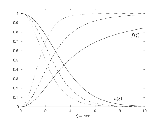
Figure 1: The monopole profile functions $u(\xi)$ and $f(\xi)$ for $\lambda/e^{2}=0$ (solid curves), $\lambda/e^{2}=0.1$ (dashed curves) and $\lambda/e^{2}=1$ (dotted curves).

The total energy of the solution, which is interpreted as the classical mass, is given by eq.(4) and to simplify the analysis we use the rescaled mass, $\tilde{E}$,

$$E=M_{0}\,\tilde{E}(\lambda/e^{2}),\quad\text{where }M_{0}=\frac{4\pi v}{e}\,.$$

Performing an analysis similar to Forgacs2005 , we can obtain the mass range for the Dark Monopoles. Note first that $\tilde{E}$ is a monotonically increasing function of $\lambda/e^{2}$, since

$$\frac{d\tilde{E}(\lambda/e^{2})}{d(\lambda/e^{2})}=\frac{1}{9|\lambda_{p}|^{4}}\,\int_{0}^{\infty}d\xi\,\xi^{2}(f^{2}-1)^{2}>0\,.$$

The lower bound for the mass happens when $\lambda=0$, and numerical integration shows that for the $SU(5)$ monopole $\tilde{E}(0)=1.294$.

Similar to the case of the ’t Hooft-Polyakov monopole KirkmanZachos , in the limit $\lambda\to\infty$ the mass of the monopole stays finite and it is given by

$$E =\frac{4\pi v}{e}\int_{0}^{\infty}d\xi\left[2(u^{\prime}_{\scaleto{\infty}{2.5pt}})^{2}+\frac{(1-u_{\scaleto{\infty}{2.5pt}}^{2})^{2}}{\xi^{2}}+\frac{l(l+1)}{3|\lambda_{p}|^{2}}\,u_{\scaleto{\infty}{2.5pt}}^{2}\right]\,,$$ (51)

since $f(\xi)\equiv 1\,\forall\,\xi>0$ but $f(0)=0$. Then, the only radial equation of motion is

$$u^{\prime\prime}_{\scaleto{\infty}{2.5pt}}=\frac{l(l+1)}{6|\lambda_{p}|^{2}}\,u_{\scaleto{\infty}{2.5pt}}+\frac{u_{\scaleto{\infty}{2.5pt}}(u_{\scaleto{\infty}{2.5pt}}^{2}-1)}{\xi^{2}}\,.$$ (52)

Solving eq.(52) and performing the integration in (51) gives us the upper bound for the monopole mass. In the $SU(5)$ case, the upper bound is $\tilde{E}(\lambda\to\infty)=3.262$. For comparison, for the ’t Hooft-Polyakov monopole in the $SU(2)$ case, $\tilde{E}(\lambda=0)=1$ PrasadSommerfield and $\tilde{E}(\lambda\to\infty)=1.787$ KirkmanZachos .

Note that for a given SSB, where $\lambda_{p}$ is fixed, the value of the mass is the same for all the Dark Monopole solutions associated to the the $su(2)$ subalgebras (18). This follows directly from the fact that the hamiltonian is independent of the indices $i,j,k$ that label those $su(2)$ subalgebras. Moreover, these are classical results. To determine the properties of the Dark Monopoles at the quantum level, one could use for example semi-classical quantization.

5 Non-abelian magnetic charge

One of the main properties of the Dark Monopole solution is that its magnetic field is in a direction outside the Cartan subalgebra $\mathcal{H}$. Thus, as we mentioned before, this monopole has vanishing abelian magnetic charge, since $\text{Tr}(B^{i}\phi)=0$. However, from eq.(13) we see that far from the monopole core it has a non-abelian magnetic flux in the direction $g(\theta,\varphi)\,M_{3}\,g^{-1}(\theta,\varphi)$, with $M_{3}$ given by eq.(18). We shall define

$$\zeta(\vec{r})=a(r)\,g(\theta,\varphi)\,M_{3}\,g^{-1}(\theta,\varphi)=a(r)\,n^{a}M_{a}\,,$$ (53)

which is in the direction of the monopole non-abelian magnetic flux, where $a(r)\in\mathbb{R}$ is a radial function such that $\zeta$ is regular everywhere. This implies that when $r\to 0$, $a(r)\sim r$. On the other hand, when $r\gg R_{core}$, we consider that $a(r)=1$. Then, using the fact that in this asymptotic region the gauge and the scalar fields assume the form (12) and (7), respectively, it is easy to verify that asymptotically $\zeta$ satisfies the conditions

$$D_{\mu}\zeta =0\,,$$ (54)

$$\left[\phi,\zeta\right] =0\,.$$ (55)

Recalling the infinitesimal form of a gauge transformation for $W_{\mu}$ and $\phi$, we can conclude that the asymptotic configuration of the monopole is invariant under a gauge transformation of the form $\exp(i\zeta)$. Therefore, $\zeta$ is a Killing vector which is associated to a symmetry of the asymptotic fields of the monopole. According to AbbottDeser and BarnichBrandt , from the existence of a Killing vector $\zeta$ for an asymptotic symmetry one can associate a conserved charge. It is interesting to note that $\zeta$ satisfies the same equations as the scalar field $\phi$ for the ’t Hooft-Polyakov monopole, outside the monopole core. Therefore, in this special case $\phi$ can be identified with the Killing vector $\zeta$. Note that if we perform an arbitrary gauge transformation $U$ on the monopole’s fields then, from eqs. (54) and (55), we obtain that $\zeta$ must transform as

$$\zeta\rightarrow\zeta^{\prime}=U\,\zeta\,U^{-1}\,,$$

in order to be a Killing vector of the transformed fields.

Moreover, since $\zeta$ and $W_{i}$ take values in the $su(2)$ subalgebra formed by $M_{a}$, we can expand them as

$$W_{i} =W_{ia}M_{a}\,,$$

$$\zeta =\zeta_{a}M_{a}\,,$$ (56)

$$D_{i}\zeta =\left(D_{i}\zeta\right)_{a}M_{a}\,,$$

where $\left(D_{i}\zeta\right)_{a}=\partial_{i}\zeta_{a}-e\epsilon_{abc}W_{ib}\zeta_{c}$. We shall also introduce the notation $\overline{\zeta}$ for the asymptotic configuration of $\zeta$. Then, it follows from eq.(53) that $\overline{\zeta}_{a}=n^{a}$ is a unitary vector. Note that $\overline{\zeta}_{a}^{2}=1$ defines a 2-sphere, which we will denote by $\Sigma$.

Now, let us define a gauge-invariant magnetic current by taking a projection of ${}^{*}G^{\mu\nu}$ in the direction of the Killing vector $\zeta$ as

$$J_{M}^{\mu}\equiv\frac{1}{|\overline{\zeta}|y}\,\partial_{\nu}\text{Tr}\left({}^{*}G^{\mu\nu}\zeta\right)\,,$$ (57)

where $|\overline{\zeta}|\equiv\sqrt{\overline{\zeta}_{a}\overline{\zeta}_{a}}=1$. Besides that, ${}^{*}G^{0i}=B^{i}$ and ${}^{*}G^{ij}=-\epsilon_{ijk}E^{k}$. The conservation of the current $J_{M}^{\mu}$ follows from its definition as a divergence of an antisymmetric tensor and from the fact that $\text{Tr}\left(B^{i}\zeta\right)$ is twice differentiable.

Thus, the conserved non-abelian magnetic charge is

$$Q_{M}=\int_{\mathbb{R}^{3}}d^{3}x\,J_{M}^{0}=\frac{1}{|\overline{\zeta}|y}\oint_{S_{\infty}^{2}}dS_{i}\,\text{Tr}\left(B^{i}\zeta\right)=-\frac{8\pi}{e}\,.$$ (58)

Note that eq.(58) is just a measure of the non-abelian flux in the normalized $\overline{\zeta}(\theta,\varphi)$ direction. Furthermore, we must emphasize that the introduction of the radial function $a(r)$ has no contribution to the magnetic charge. This artifact was introduced so that we could define a regular magnetic current for the Dark Monopole. Besides that, as pointed out by Coleman_Aspects there is no unambiguous way to measure the charge density of a monopole. Only the total charge makes sense.

Let us now analyze the geometric meaning of the magnetic charge (58). From the asymptotic condition (54) it follows that

$$\frac{1}{8\pi y}\epsilon^{ijk}\oint_{S_{\infty}^{2}}dS_{i}\textrm{Tr}\left\{\zeta\left[D_{j}\zeta,D_{k}\zeta\right]\right\}=0\,.$$ (59)

Then, from eq.(56) and using vector notation, as well as the fact that $|\zeta|=1$ when $r\to\infty$, eq.(59) can be written as

$$\frac{1}{8\pi}\epsilon^{ijk}\oint_{S_{\infty}^{2}}dS_{i}\left\{\hat{\zeta}\cdot\left(\partial_{j}\hat{\zeta}\times\partial_{k}\hat{\zeta}\right)-e\hat{\zeta}\cdot\overrightarrow{G}_{jk}\right\}=0\,.$$ (60)

Now, using eq.(23a) the expression of the non-abelian magnetic charge (58) can be written as

$$Q_{M}=2\,\oint_{S_{\infty}^{2}}dS_{i}\overrightarrow{B}^{i}\cdot\hat{\zeta}\,,$$

and from eq.(60) we conclude that

$$Q_{M}=-\frac{4\pi}{e}\,2N_{\zeta}\,,$$

where

$$N_{\zeta}=\frac{1}{8\pi}\epsilon^{ijk}\oint_{S_{\infty}^{2}}dS_{i}\left\{\hat{\zeta}\cdot\left(\partial_{j}\hat{\zeta}\times\partial_{k}\hat{\zeta}\right)\right\}\,.$$

As it is well-known, this integral is a topological quantity which is an integer and has the geometrical interpretation ArafuneFredGoebel which is to measure the number of times $\hat{\zeta}$ covers $\Sigma$ as $\hat{r}$ covers $S_{\infty}^{2}$ once. For our particular Dark Monopole construction, where $\bar{\zeta}^{a}=n^{a}$, $N_{\zeta}=1$. However, in principle, one could obtain higher magnetic charges, generalizing our construction, considering for example a gauge transformation

$$g(\theta,\varphi)=\exp\left(-i\varphi kM_{3}\right)\exp\left(-i\theta M_{2}\right)\exp\left(i\varphi kM_{3}\right),\quad k\in\mathbb{Z}\,,$$

which would be associated to $\hat{\zeta}$ covering $\Sigma$ $k$ times as $\hat{r}$ covers $S_{\infty}^{2}$ once.

It is important to remark that for the Dark Monopole, the magnetic charge is not the usual one (in the abelian direction), associated to the homotopy classes of the scalar field, like in the ’t Hooft-Polyakov case.

Therefore, from the results above we can conclude that the non-abelian magnetic charge of the Dark Monopole is conserved and quantized in multiples of $8\pi/e$. And even though they are associated to the trivial sector of $\Pi_{1}(G_{v})$, the conservation of $Q_{M}$ could prevent them to decay, at least classically. However, it is necessary to analyze in more detail the stability of the Dark Monopole.

6 Discussions and Conclusion

In this work we have obtained a general procedure to construct magnetic monopole solutions, which we call Dark Monopoles, since their magnetic field vanishes in the direction of the generator of the $U(1)_{em}$ electromagnetic field. In order to do that, we considered theories with gauge group $SU(n)$ and a scalar in the adjoint representation. But we expect that this construction can be generalized to other gauge groups. These Dark Monopoles must exist in some Grand Unified Theories and we analyzed some of their properties for the $SU(5)$ case. In particular, we obtained their mass range.

We also have shown that our monopole solution has a conserved magnetic current $J^{\mu}_{M}$ in the direction of the Killing vector $\zeta$. The associated charge is quantized and it measures the number of times $\hat{\zeta}$ covers $\Sigma$ as $\hat{r}$ covers $S_{\infty}^{2}$ once. In principle, the conservation of this non-abelian magnetic charge could prevent the Dark Monopoles to decay. However, the stability should be analyzed in more detail in the future. Nonetheless, in order to discuss some cosmological aspects, let us assume for a moment that our solution is indeed stable or has a reasonable lifetime.

We expect that the Dark Monopoles were created in a phase transition in the early universe by the Kibble mechanism at a temperature of the order of the unification scale, along with the standard GUT monopoles. Under some general assumptions KolbTurner one can show that their initial abundance $n_{M}(t_{i})$ has evolved in time according to Preskill

$$\dot{n}_{M}+3Hn_{M}=-Dn_{M}^{2}\,,$$

where $H\equiv\dot{a}/a$ is the Hubble parameter, while $a(t)$ is the scale factor in the Robertson-Walker metric. The last term is associated to the annihilation mechanism and comes from the collision term in the Boltzmann equation. This implies that the time evolution of the monopole density strongly depends on how the monopoles interact between themselves and also on how they interact with the plasma of particles in the universe. Their motion can be described as VilenkinShellard a Brownian motion of heavy dust particles in a gas or liquid with a slight bias in their random walks caused by the interaction between monopoles and antimonopoles. But one should note that since our monopoles have a vanishing $U(1)$ magnetic charge, there may be some differences in the annihilation mechanism, such as a different mean free path $l$ and capture radius $r_{c}$ (high-temperature regime) as well as the cross-section for radiative capture (low-temperature regime). As a consequence, we expect the so called monopole-to-entropy ratio VilenkinShellard ; WeinbergBook to be different. However, a future detailed analysis on how the monopoles interact is necessary in order to make estimates of this ratio.

Another relevant point is that when some possible ordinary monopoles interact with the magnetic field of our galaxy, they are accelerated. And it depends on the mass of these monopoles whether they will be ejected or slightly deflected WeinbergBook . In any case, the acceleration of these monopoles will drain energy from the galactic field. Now, note that since our Dark Monopoles do not interact with galactic magnetic fields, they will not be accelerated and, in principle, this means that they can cluster with the galaxy. The same reasoning can be applied to magnetic fields in galactic clusters.

Now, with regard to the Dark Matter problem we expect that Dark Monopoles might contribute to part of the mass usually attributed to Dark Matter. However, in face of the inflationary scenario, we expect that this contribution might be small. One way out of this is to investigate whether it is possible that any amount of Dark Monopoles were created during the reheating phase after inflation through energy density fluctuations. Although even if they do not have a relevant contribution to Dark Matter, they are still an interesting solution since they are a new type of GUT monopoles.

Finally, we recall that as the case of standard GUT monopoles the mass of our Dark Monopoles is set by the GUT scale, which is beyond the energy scale of particle physics experiments, and currently direct detection is unlikely. However, as we mentioned before, further analysis is needed on how our monopoles interact and this may give some hints on the way we can look for them.

- (1) G. ’t Hooft, Magnetic Monopoles in Unified Gauge Theories, Nuc. Phys. B 79 (1974) 276 [inSPIRE].
- (2) A. M. Polyakov, Particle Spectrum in the Quantum Field Theory, JETP Lett. 20 (1974) 194 [inSPIRE].
- (3) E. Corrigan and D. Olive, Color and Magnetic Monopoles, Nucl. Phys. B 110 (1976) 237 [inSPIRE].
- (4) P. Goddard and D. I. Olive, Magnetic Monopoles in Gauge Field Theories, Rept. Prog. Phys. 41 (1978) 1357 [inSPIRE].
- (5) P. Goddard and D. I. Olive, Charge Quantization in Theories with an Adjoint Representation Higgs Mechanism, Nuc. Phys. B 191 (1981) 511 [inSPIRE].
- (6) C.P. Dokos and T.N. Tomaras, Monopoles and dyons in SU(5) model, Phys. Rev. D 21 (1980) 2940 [inSPIRE].
- (7) G. B. Gelmini, The Hunt for Dark Matter, in Proceedings of the 2014 Theoretical Advanced Study Institute in Elementary Particle Physics, Boulder, Colorado, June 2014. [hep-ph/1502.01320v2] [inSPIRE].
- (8) K. Freese, Status of Dark Matter in the Universe, Int.J.Mod.Phys. 1 (2017) 325 [astro-ph.CO/1701.01840v1] [inSPIRE].
- (9) C. G. Sanchez and B. Holdom, Monopoles, Strings and Dark Matter, Phys. Rev. D 83 (2011) 123524 [hep-ph/1103.1632v2] [inSPIRE].
- (10) V. V. Khoze and G. Ro, Dark matter monopoles, vectors and photons, JHEP 10 (2014) 061 [hep-ph/1406.2291v3] [inSPIRE].
- (11) S. Baek, P. Ko and Wan-Il Park, Hidden sector monopole, vector dark matter and dark radiation with Higgs portal, JCAP 10 (2014) 067 [hep-ph/1311.1035v2] [inSPIRE].
- (12) J. Evslin, Spiked Monopoles, JHEP 03 (2018) 143 [hep-th/1801.04206v1] [inSPIRE].
- (13) R. Sato, F. Takahashi and M. Yamada, Unified Origin of Axion and Monopole Dark Matter, and Solution to the Domain-wall Problem, [hep-ph/1805.10533v1] [inSPIRE].
- (14) G. Lazarides and Q. Shafi, Monopoles, axions and intermediate mass dark matter, Phys. Lett. B 489 (2000) 194 [hep-ph/0006202v2] [inSPIRE].
- (15) H. Murayama and J. Shu, Topological Dark Matter, Phys. Lett. B 686 (2010) 162 [hep-ph/0905.1720v1] [inSPIRE].
- (16) E. Corrigan, D. I. Olive, D. B. Fairlie and J. Nuyts, Magnetic Monopoles in Gauge Theories, Nucl. Phys. B 106 (1976) 475 [inSPIRE].
- (17) J. Burzlaff, monopoles with magnetic quantum numbers , Phys. Rev. D 23 (1981) 1329 [inSPIRE].
- (18) J. Kunz and D. Masak, Finite-energy monopoles, Phys. Lett. B 196 (1987) 513 [inSPIRE].
- (19) S. Coleman, The Magnetic Monopole Fifty Years Later. In: Zichichi A. (eds) The Unity of the Fundamental Interactions, Springer, (1983) [inSPIRE].
- (20) E. J. Weinberg, D. London and J. L. Rosner, Magnetic Monopoles with Charges, Nuc. Phys. B 236 (1984) 90 [inSPIRE].
- (21) F. A. Bais, Charge-monopole duality in spontaneously broken gauge theories, Phys. Rev. D 18 (1978) 1206 [inSPIRE].
- (22) E. J. Weinberg, Fundamental Monopoles in Theories With Arbitrary Symmetry Breaking, Nucl. Phys. B 203 (1982) 445 [inSPIRE].
- (23) F.A. Bais and B.J. Schroers, Quantisation of monopoles with non-abelian magnetic charge, Nuc. Phys. B 512 (1998) 250 [hep-th/9708004v2] [inSPIRE].
- (24) B.J. Schroers and F.A. Bais, S-duality in Yang-Mills theory with non-abelian unbroken gauge group, Nuc. Phys. B 535 (1998) 197 [hep-th/9805163v2] [inSPIRE].
- (25) M. A. C. Kneipp and P. J. Liebgott, monopoles in Yang-Mills-Higgs theories, Phys. Rev. D 81 (2010) 045007 [hep-th/0909.0034v2] [inSPIRE].
- (26) M. A. C. Kneipp and P. J. Liebgott, BPS monopoles and superconformal field theories on the Higgs branch, Phys. Rev. D 87 (2013) 025024 [hep-th/1210.7243v2] [inSPIRE].
- (27) M. Aryal and A. E. Everett, Properties of Z(2) Strings, Phys. Rev. D 35, (1987) 3105. [inSPIRE].
- (28) C.P. Ma, cosmic strings and baryon number violation, Phys. Rev. D 48 (1993) 530 [hep-ph/9211206v1] [inSPIRE].
- (29) A. Vilenkin and E.P.S. Shellard, Cosmic Strings and Other Topological Defects, Cambridge University Press, (1994) [inSPIRE].
- (30) M. B. Hindmarsh and T. W. B. Kibble, Cosmic strings, Rept. Prog. Phys. 58 (1995) 477. [hep-ph/9411342] [inSPIRE].
- (31) A.C. Davis and S.C. Davis, Microphysics of cosmic strings, Phys. Rev. D 55 (1997) 1879 [hep-th/9608206v2] [inSPIRE].
- (32) T. W. B. Kibble, G. Lozano, and A. J. Yates, Non-Abelian string conductivity, Phys. Rev. D 56 (1997) 1204. [hep-ph/9701240] [inSPIRE].
- (33) M.A.C. Kneipp and P.J. Liebgott, New strings, Phys.Lett. B 763 (2016) 186. [1610.01654v2] [inSPIRE].
- (34) S. Helgason, Differential Geometry, Lie Groups and Symmetric Spaces, Academic Press, INC., (1978).
- (35) Wu-Ki Tung, Group Theory in Physics, World Scientific, (1985).
- (36) A. Abouelsaood, Are there chromodyons?, Nuc. Phys. B 226 (1983) 309 [inSPIRE].
- (37) A. Abouelsaood, Chromodyons and Equivariant Gauge Transformations, Phys. Lett. B 125 (1983) 467 [inSPIRE].
- (38) A.P. Balachandran, G. Marmo, N. Mukunda, J.S. Nilsson, E.C.G. Sudarshan and F. Zaccaria, Monopole Topology and the Problem of Color, Phys. Rev. Lett. 50 (1983) 1553 [inSPIRE].
- (39) A.P. Balachandran, G. Marmo, N. Mukunda, J.S. Nilsson, E.C.G. Sudarshan and F. Zaccaria, Non-Abelian monopoles break color. I. Classical mechanics, Phys. Rev. D 29 (1984) 2919 [inSPIRE].
- (40) A.P. Balachandran, G. Marmo, N. Mukunda, J.S. Nilsson, E.C.G. Sudarshan and F. Zaccaria, Non-Abelian monopoles break color. II. Field theory and quantum mechanics, Phys. Rev. D 29 (1984) 2936 [inSPIRE].
- (41) P. Nelson and A. Manohar, Global Color Is Not Always Defined, Phys. Rev. Lett. 50 (1983) 943 [inSPIRE].
- (42) P. Nelson and S. Coleman, What Becomes of Global Color?, Nuc. Phys. B 237 (1984) 1 [inSPIRE].
- (43) P.A. Horvathy and J.H. Rawnsley, Internal Symmetries of Nonabelian Gauge Field Configurations, Phys. Rev. D 32 (1985) 968 [inSPIRE].
- (44) P.A. Horvathy and J.H. Rawnsley, The Problem of ’Global Color’ in Gauge Theories, J. Math. Phys. 27 (1986) 982 [inSPIRE].
- (45) P. Irwin, SU(3) monopoles and their fields, Phys. Rev. D 56 (1997) 5200 [hep-th/9704153v2] [inSPIRE].
- (46) E. B. Bogomolny, Stability of Classical Solutions, Sov.J.Nucl.Phys. 24 (1976) 449 [inSPIRE].
- (47) R. G. Barrera, G. A. Estévez and J. Giraldo, Vector spherical harmonics and their application to magnetostatics, Eur. J. Phys. 6 (1985) 287 [doi].
- (48) P. Forgács, N. Obadia and S. Reuillon, Numerical and asymptotic analysis of the ’t Hooft-Polyakov magnetic monopole, Phys. Rev. D 71 (2005) 035002 [hep-th/0412057v2] [inSPIRE].
- (49) T. W. Kirkman and C. K. Zachos, Asymptotic Analysis of the Monopole Structure, Phys. Rev. D 24 (1981) 999 [inSPIRE].
- (50) M.K. Prasad and C. M. Sommerfield, An Exact Classical Solution for the ’t Hooft Monopole and the Julia-Zee Dyon, Phys. Rev. Lett. 35 (1975) 760 [inSPIRE].
- (51) L. F. Abbott and S. Deser, Charge Definition in Nonabelian Gauge Theories, Phys. Lett. B 116 (1982) 259 [inSPIRE].
- (52) G. Barnich and F. Brandt, Covariant theory of asymptotic symmetries, conservation laws and central charges, Nuc. Phys. B 633 (2002) 3 [hep-th/0111246v2] [inSPIRE].
- (53) S. Coleman, Aspects of Symmetry, Cambridge University Press, (1985).
- (54) J. Arafune, P.G.O. Freund and C.J. Goebel, Topology of Higgs Fields, J. Math. Phys. 16 (1975) 433 [inSPIRE].
- (55) E. Kolb and M. Turner, The Early Universe, Addison-Wesley Publishing Company, (1990).
- (56) J. Preskill, Cosmological Production of Superheavy Magnetic Monopoles, Phys. Rev. Lett. 43 (1979) 1365 [inSPIRE].
- (57) E.J. Weinberg, Classical Solutions in Quantum Field Theory: Solitons and Instantons in High Eneergy Physics, Cambridge University Press, (2012) [inSPIRE].