Solving integral equations in $\eta\to 3\pi$

Abstract

A dispersive analysis of $\eta\to 3\pi$ decays has been performed in the past by many authors. The numerical analysis of the pertinent integral equations is hampered by two technical difficulties: i) The angular averages of the amplitudes need to be performed along a complicated path in the complex plane. ii) The averaged amplitudes develop singularities along the path of integration in the dispersive representation of the full amplitudes. It is a delicate affair to handle these singularities properly, and independent checks of the obtained solutions are demanding and time consuming. In the present article, we propose a solution method that avoids these difficulties. It is based on a simple deformation of the path of integration in the dispersive representation (not in the angular average). Numerical solutions are then obtained rather straightforwardly. We expect that the method also works for $\omega\to 3\pi$.

1 Introduction

The study of the $\eta\to 3\pi$ decay process is interesting, first and foremost, in the context of the determination of the quark mass ratio

$$Q^{2}=\frac{m_{s}^{2}-\hat{m}^{2}}{m_{d}^{2}-m_{u}^{2}}\,,\quad\quad\hat{m}=\frac{1}{2}\,(m_{u}+m_{d})\,.$$ (1)

In order to extract the value of $Q$ to high precision, it is very important to have a robust control on the final–state interactions in this decay, which lead to a strong effect in the width. To this end, one would like to have a non–perturbative framework, allowing the resummation of a certain class of the final–state interactions to all orders. Dispersion relations are the ideal tool for this. Incorporating 2–particle unitarity and crossing symmetry then leads to a system of coupled integral equations for the 3 isospin amplitudes in this decay. It took quite some time until these equations were written down in their final form. The development started with the pioneering work of Khuri and Treiman Khuri:1960zz . The mathematical structure of this type of equation was investigated in the following decade Gribov:1962fu ; Bonnevay ; Bronzan:1963mby ; Kacser:1963zz ; Bronzan:1964zz ; Aitchison:1964zz ; Aitchison:1965zz ; Pasquier:1968zz ; Pasquier:1969dt , see also the monograph Anisovich:2013gha . Later, interest in the dispersive method waned. A revival occurred in the nineties, when it was demonstrated Anisovich:1993kn ; Kambor:1995yc ; Anisovich:1996tx ; Walker how dispersion relations allow one to incorporate final state interactions of S- and P-waves in a reliable and calculable manner. Refs. Kambor:1995yc ; Anisovich:1996tx contain a detailed discussion of the role of subtractions in the dispersive representation, while the uniqueness of the solutions is investigated in Anisovich:1996tx . Further, current algebra Osborn:1970nn and chiral perturbation theory results Gasser:1984pr were used to relate the parameter $Q$ to this framework (normalization of the dispersive amplitude), and to get a handle on the subtraction constants. For a review of the early developments until 1990 we refer the reader to Ref. Anisovich:1993kn , see also the lecture notes Aitchison:2015jxa . An improved representation of the $\pi\pi$ phase shifts Colangelo:2001df ; Kaminski:2006qe , the evaluation of electromagnetic corrections Bissegger:2008ff ; Ditsche:2008cq as well as new experimental information on this decay Ambrosino:2008ht ; Prakhov:2008ff ; Unverzagt:2008ny ; Ambrosinod:2010mj ; Adlarson:2014aks ; Ablikim:2015cmz ; Anastasi:2016cdz ; Prakhov:2018tou triggered new investigations of $\eta\to 3\pi$ in the dispersive framework Lanz_phd ; Colangelo:2011zz ; Lanz:2013ku ; Descotes-Genon:2013uya ; Descotes-Genon:2014tla ; Guo:2015zqa ; Albaladejo:2015bca ; Moussallam:2016evb ; Guo:2016wsi ; Colangelo:2016jmc ; Albaladejo:2017hhj . A very comprehensive analysis has recently been presented in Ref. Colangelo:2018jxw . For applications of the dispersive framework in other three–body decays, see Refs.Niecknig:2012sj ; Descotes-Genon:2013uya ; Descotes-Genon:2014tla ; Niecknig:2015ija ; Niecknig:2016fva ; Isken:2017dkw ; Niecknig:2017ylb . Further attempts to incorporate a class of final state interactions in the $\eta\to 3\pi$ amplitudes may be found in Refs. Roiesnel:1980gd ; Gasser:1984pr ; Bijnens:2002qy ; Bijnens:2007pr ; Schneider:2010hs ; Schneider:2013phd .

The present article is devoted to a discussion of numerical methods to solve the integral equations that occur in the formulation of Ref. Colangelo:2018jxw . In this connection, the investigations  Gribov:1962fu ; Bonnevay ; Bronzan:1963mby ; Kacser:1963zz ; Bronzan:1964zz ; Aitchison:1964zz ; Aitchison:1965zz ; Pasquier:1968zz ; Pasquier:1969dt revealed the following two important aspects:

1. In the evaluation of the angular averages of the amplitudes, the integration path in $z=\cos\theta$ must be deformed into the complex plane, in order not to destroy the holomorphic properties of the amplitudes. The deformation is fixed by providing the (eta mass)² with an infinitesimal positive imaginary part: $M_{\eta}^{2}\to M^{2}=M_{\eta}^{2}+i\delta$ , with $\delta\to 0^{+}$ at the end of the calculation.

2. Singularities emerge in the angular averaged amplitudes, at the pseudothreshold $s=(M_{\eta}-M_{\pi})^{2}$. Some of these singularities are of a non–integrable type in the Lebesgue sense. The (positive) imaginary part of the eta mass, however, acts as a regulator, that can be removed after the dispersive integral has been performed. Handling these singularities properly is a delicate affair, as is illustrated e.g. by the discussions in Refs.Kambor:1995yc ; Walker ; Lanz_phd ; Descotes-Genon:2014tla ; Schneider:2013phd ; Niecknig:2016fva ; Albaladejo:2017hhj ; Colangelo:2018jxw .

We shortly mention several previous methods to obtain solutions of these equations. In Refs. Kambor:1995yc ; Walker ; Lanz_phd ; Colangelo:2011zz ; Lanz:2013ku ; Niecknig:2012sj ; Colangelo:2018jxw , the equations were solved directly through iterations, with a careful treatment of the mentioned singularities. In Ref. Descotes-Genon:2014tla ; Albaladejo:2017hhj , integral kernels are introduced, which make the numerical procedure faster, and which identify the mentioned singularities at the pseudothreshold in a clear fashion. Through the interchange of the order of integrations, the so–called Pasquier inversion Pasquier:1968zz ; Pasquier:1969dt , it is possible to carry out one integration and to obtain integral equations in one variable that are further solved by iterations (see Refs. Guo:2014mpp ; Guo:2014vya ; Guo:2015zqa ; Guo:2016wsi for more details). Finally, it is possible to obtain integral equations for the angular averaged amplitudes instead of the amplitudes themselves. This technique has recently been invoked in Refs. Niecknig:2015ija ; Niecknig:2016fva . Last but not least, the convergence of the iterative procedure to solve the equations is not a priori guaranteed. The iterative procedure converges very well (typically, after 3–4 iterations) in the $\eta\to 3\pi$ decays, but the convergence becomes an issue for decaying particles with heavier masses, or for equations with more subtractions Niecknig:2016fva . For this reason, e.g., in Ref. Niecknig:2015ija , a matrix inversion method was used to find a solution beyond the iterative procedure. These enterprises are numerically very demanding, in particular for the reasons spelled out above.

In the following, we propose a numerical framework that avoids the difficulties i) and ii) altogether. We show that one may deform the integration path in the dispersion integral (not in the angular average) into the complex plane. After choosing a properly deformed path, the integrand becomes regular, even at $\delta=0$ (except at threshold, where a mild, integrable square root singularity persists). In addition, the angular integration can be carried out in the original interval $-1\leq z\leq 1$. Further, discretizing the integrals through a Gauss–Legendre quadrature, the integral equations are transformed into a set of linear matrix equations, whose solution is easily found by iterations. The procedure is pretty straightforward, takes very little CPU time and does not lead to any spurious irregularities in the solutions.

The idea to avoid singularities in integration through path deformation is not new. An early reference is the work of Hadamard Hadamard:1898 , whose method was rediscovered 50 years later by investigation of analytic properties of perturbation theory Eden:1952 ; Smatrix:1966 , and then extended and extensively used in S-matrix theory Smatrix:1966 . The analogue of the procedure for the quantum–mechanical three–body problem is well known since decades Hetherington:1965zza ; Schmid . As already said, Aitchison and Pasquier mentioned this possibility for Khuri-Treiman-type equations in Ref. Aitchison:1966lpz . For the numerical evaluation of loop graphs in Quantum Field Theory, path deformations in momentum space Soper:1998ye as well as in Feynman parameter space Nagy:2006xy are used. All these techniques, including the present one, may be summarized under the heading “Applications of Cauchy’s integral theorem”.

The layout of the article is as follows. In section 2, we display the integral equations for the $\eta\to 3\pi$ amplitudes in the form worked out recently in Ref. Colangelo:2018jxw . We describe in some details the technical difficulties that one encounters while solving the equations in section 3, while in section 4, we define the deformed path in the dispersion integral and show that in this manner, the singularities in the integral equations disappear. In section 5 we describe the numerical procedure for solving the equations, whereas a summary and conclusions are given in section 6. In appendix A we comment on the phase shifts used and collect some notation. The holomorphic continuation of the integrand is discussed in appendix B, path deformations in general are investigated in appendix C, and the case $\omega\to 3\pi$ is shortly discussed in appendix D.

2 The equations

We start from the integral equations for the three isospin amplitudes $M_{I}(s)$ in the framework specified in Colangelo:2018jxw ,

$$M_{I}(s) = \Omega_{I}(s)\left[P_{I}(s)+s^{n_{I}}\int_{4M_{\pi}^{2}}^{\infty}d\mu_{I}(x)\frac{\hat{M}_{I}(x)}{x-s-i\epsilon}\right]\,,$$ (2)

$$I=0,1,2\,.$$

The various quantities are defined as follows. The Omnès functions are

$$\Omega_{I}(s)=\exp\left(\frac{s}{\pi}\int_{4M_{\pi}^{2}}^{\infty}\frac{dx}{x}\frac{\delta_{I}(x)}{x-s-i\epsilon}\right),$$ (3)

where $\delta_{I}(x)$ denote the elastic $\pi\pi$ phase shifts (S-wave for $I=0,2$, P-wave for $I=1$). The hat–functions $\hat{M}_{I}$ are defined in terms of angular averages,

$$\hat{M}_{I}(x)=\frac{1}{\kappa}\sum_{m,I^{\prime}}C^{m}_{II^{\prime}}(x,\kappa)\langle z^{m}M_{I^{\prime}}\rangle(x),$$

with

$$\langle z^{m}M_{I}\rangle(x) = \frac{1}{2}\int_{-1}^{1}dzz^{m}M_{I}(h(x,z))\,;$$ (4)

$$I,I^{\prime},m\in\{0,1,2\}\,,$$

where

$$h(x,z)=\frac{1}{2}\left[M^{2}+3M_{\pi}^{2}-x+z\,\kappa(M^{2},M_{\pi}^{2},x)\right],$$

$$\kappa(M^{2},M_{\pi}^{2},x)=\sqrt{1-\frac{4M_{\pi}^{2}}{x}}\sqrt{x-(M-M_{\pi})^{2}}$$

$$\hskip 61.17325pt\times\sqrt{x-(M+M_{\pi})^{2}}\,.$$ (5)

Finally, the measures are

$$d\mu_{I}(x)=\frac{dx}{\pi x^{n_{I}}}\frac{\sin(\delta_{I}(x))}{|\Omega_{I}(x)|},$$

and

$$\{n_{0},n_{1},n_{2}\}=\{2,1,2\}\,;$$

$$M^{2}=M_{\eta}^{2}+i\delta\,,\quad\delta\to 0^{+}\,.$$ (6)

The $C^{m}_{II^{\prime}}(x,\kappa)$ are polynomials in $x$ and $\kappa$, and $P_{I}(s)$ denote subtraction polynomials, see Colangelo:2018jxw . The phase shifts $\delta_{I}$ are needed as input to solve these equations. We relegate a discussion of them to the appendix A, where we also collect some of the notation used below.

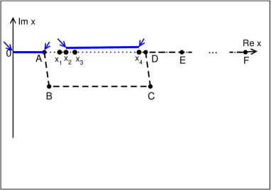
Figure 1: Branch points (blue arrows) and cuts (solid blue) of the Kacser function $\kappa(M^{2},M_{\pi}^{2},x)$, and integration paths. We connect the branch points with cuts in the intervals $[0,4M_{\pi}^{2}]$ and $[(M-M_{\pi})^{2},(M+M_{\pi})^{2})]$. The original path of integration for the dispersive representation (2) runs along the real line, from A to DEF (dotted black), the deformed path along ABCDEF (dashed black). See appendix A for $x_{i}$ and $A,B,\ldots F$. The figure is not drawn on scale.

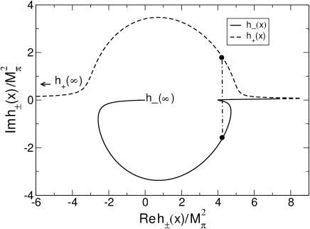
Figure 2: Real and imaginary parts of the endpoints $h_{\pm}(x)$ in (7) in the angular averages (4), for $x\in[4M_{\pi}^{2},\infty)$. For better visibility, we have kept in the eta mass a positive imaginary part. Solid (dashed) line: lower (upper) endpoint. The dash–dotted line connects $h_{-}(x)$ with $h_{+}(x)$, with $x_{2}\!<\!x\!<\!x_{3}$. It is seen that this line crosses the original path of integration in the dispersive representation (2). The same happens for $x_{1}\!<\!x\!<\!x_{2}$. See text for details.

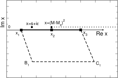
Figure 3: Integration paths for the singular integral $G(s)$ in (4). The original path runs along the real line, from $x_{1}$ to $x_{3}$ (solid line). The upper horizontal line (dotted) stands for the cut attached to the branch point at $x=(M-M_{\pi})^{2}$. The two singularities of the integrand are indicated with filled circles. Since these are located in the upper complex plane, the path may be deformed into the lower half plane, e.g., into the polygonal line $x_{1}B_{1}C_{1}x_{3}$ (dashed line), without changing the value of the integral. See appendix A for $x_{i},B_{1},C_{1}$.

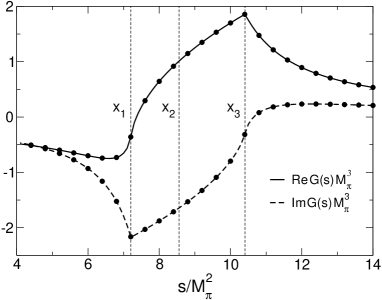
Figure 4: Analytical and numerical results for the function $G(s)$ in Eq. 4. The solid and dashed lines denote the real and imaginary part of the analytical result Colangelo:2018jxw , the filled circles denote the result from the Gauss-Legendre integration along the polygonal line $x_{1}B_{1}C_{1}x_{3}$ in Fig.(3).

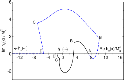
Figure 5: Real and imaginary part of the endpoints $h_{\pm}(x)$ in (7), if the integration in the dispersive integral (2) is performed along the deformed path ABCDEF in Fig. 1. Compare with Fig. 2, which shows the situation in the standard case.

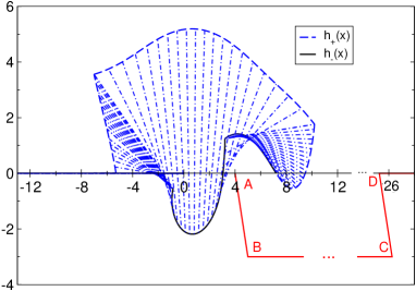
Figure 6: Displayed are some straight lines (dash–dotted) that connect the lower and upper ends $h_{\pm}(x)$ in the angular averages (4), see also Fig. 5. Axes in units of $M_{\pi}^{2}$. The eta mass is real. It is seen that the dash–dotted lines do not cross the path ABCD and hence they stay within the holomorphy domain of the amplitudes $M_{I}(s)$. One can therefore perform the angular averages in their original form.

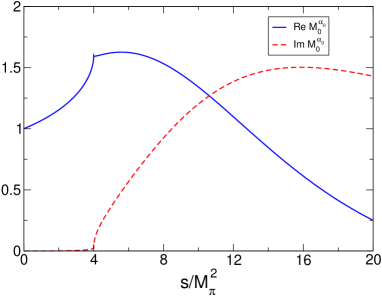
Figure 7: Solution of the isospin zero amplitude. Notation as in Ref. Colangelo:2018jxw .

3 Technical hurdles

During the numerical, iterative solution of the equations (2)-(2), two main problems occur.

i) The angular averages $\langle z^{m}M_{I}\rangle(x)$ amount to an integration along the path $h(x,z)$ of the argument of the amplitudes $M_{I}$. For fixed $x$, the argument runs along a straight line, from $h_{-}(x)$ to $h_{+}(x)$, where

$$h_{\pm}(x)=\frac{1}{2}\left[M^{2}+3M_{\pi}^{2}-x\mp\kappa(M^{2},M_{\pi}^{2},x)\right]\,.$$ (7)

The Kacser function $\kappa(M^{2},M_{\pi}^{2},x)$ Kacser:1963zz is holomorphic in the complex $x$–plane, cut along the real axis from $x=0$ to $x=4M_{\pi}^{2}$ and along a straight line from $x=(M-M_{\pi})^{2}$ to $x=(M+M_{\pi})^{2}$ , see Fig. 1. Therefore, fixing its value at some point in the complex $x$–plane renders it unique in the cut plane. In the following, we use the convention

$$\kappa(M^{2},M_{\pi}^{2},x)=x+O(1)\,,x\to\infty\,.$$ (8)

In Fig. 2, we display the endpoints $h_{\pm}(x)$ as the integration variable $x$ runs from the threshold to infinity. Because $\kappa(M^{2},M_{\pi}^{2},x)$ is holomorphic in the cut $x$ plane, the endpoints $h_{\pm}$ move – for $\delta>0$ – along curves that are infinitely often differentiable with respect to the real variable $x$. The dash–dotted vertical line connects the endpoints $h_{\pm}(x)$ with $x_{2}\!<\!x\!<\!x_{3}$. It is seen that a straight line between $h_{-}(x)$ and $h_{+}(x)$ crosses the integration path in the dispersive representation (2). This is also the case for $x_{1}\!<\!x\!<\!x_{2}$. The problem is discussed at many places in the literature – early references are Gribov:1962fu ; Bronzan:1963mby . Its solution amounts to deform the path in the $z$ integration (or in the integration over the variable $h$ after a change of variables $z\to h$), such that this crossing is avoided. We do not discuss this point any further here.

ii) The second problem arises after the angular integration has been performed in one way or the other. The angular averages develop singularities of the type

$$\hat{M_{I}}(x)\sim\frac{K}{[(M-M_{\pi})-x)]^{p}}\,,$$ (9)

where $p=(\frac{1}{2},\frac{3}{2},\frac{1}{2})$ for $I=(0,1,2)$, and $K$ denotes a constant. These singularities then show up in the dispersive integrals (2). It turns out that, after the integration over $x$ has been performed, the limit $M\to M_{\eta}$ exists. [See e.g. Refs. Kambor:1995yc ; Colangelo:2018jxw , where the dispersive integral has been worked out explicitly.] We note that the case $p=\frac{3}{2}$ corresponds to a non–integrable singularity at $\delta=0$: one is not allowed to interchange the limit $\delta\to 0^{+}$ with the integration over $x$. These singularities render the standard procedure to construct a numerical solution of the integral equations rather delicate and cumbersome. In the following, we present a method to solve these equations in an easy and straightforward manner, that avoids the problems i) and ii) altogether. [Including higher partial waves leads to even stronger singularities kubis_private . Our method also covers these cases, see the following section.]

4 Avoiding singular integrals

There is a simple way to cope with the singularities of the angular averages. To illustrate, we consider the integral Kambor:1995yc ; Colangelo:2018jxw

$$G(s)=\int_{x_{1}}^{x_{3}}\frac{g(x)\,dx}{(x-s-i\epsilon)((M-M_{\pi})^{2}-x)^{3/2}}\,,$$

$$g(x)=\frac{(x-x_{1})(x_{3}-x)}{(x_{2}-x_{1})(x_{3}-x_{2})}\,.$$ (10)

We display in Fig. 3 the singularities of the integrand with two black dots in the complex $x$-plane: one at $x=s+i\epsilon$, the second at $x=(M-M_{\pi})^{2}\stackrel{{\scriptstyle\delta\to 0^{+}}}{{\rightarrow}}x_{2}$. We have also drawn a cut that emerges from the branch point at this second singularity, reaching out to $x=\infty+i\delta$ (dotted line). The path of integration is indicated with a solid line, from $x_{1}$ to $x_{3}$. We now observe that the integrand is holomorphic in the complex half–plane Im$(x)\!<\!\epsilon,\delta$. Therefore, we may deform the path of integration into the polygonal line $x_{1}B_{1}C_{1}X_{3}$ (dashed), without changing the value of the integral. There are then no singularities anymore on the integration path, and we may set $\epsilon=\delta=0$ before performing the integration. This proves that the limit $\epsilon,\delta\to 0^{+}$ of the original integral (4) exists Kambor:1995yc ; Colangelo:2018jxw . [It is obvious that this remains true if the exponent $3/2$ in (4) is replaced by any $p\in{\mathchoice{\hbox{\hbox to0.0pt{\kern 2.88884pt\vrule height=6.14993pt\hss}\hbox{$\displaystyle\sf C$}}}{\hbox{\hbox to0.0pt{\kern 2.88884pt\vrule height=6.14993pt\hss}\hbox{$\textstyle\sf C$}}}{\hbox{\hbox to0.0pt{\kern 2.02219pt\vrule height=4.30496pt\hss}\hbox{$\scriptstyle\sf C$}}}{\hbox{\hbox to0.0pt{\kern 1.44441pt\vrule height=3.07497pt\hss}\hbox{$\scriptscriptstyle\sf C$}}}}$.] On the other hand, approaching the real axis from below, one encounters a pinch singularity at $s=(M-M_{\pi})^{2}$, which results in a singular behaviour of the function $G(s)$.

A numerical integration along the dashed path does not pose any problems, because the integrand is smooth as a function of $x$. To illustrate, we display in Fig. 4 the real part (solid line) and imaginary part (dashed line) of the function $G(s)$ (analytic expression is given in Colangelo:2018jxw ), in units of the pion mass. For comparison, the result of the numerical integration along the dashed polygonal line with 160 Gauss-Legendre points is shown with filled circles. It is seen that the agreement is perfect.

We now use the same method in the original equations (2). Suppose that the integrand in (2) is holomorphic in some region Im($x)\!<\!0$ (we discuss this point in appendix B). Then we can avoid the singularities generated by the zeros in the function $\kappa(M^{2},M_{\pi}^{2},x)$ by deforming the path as shown in Fig 1. Aside from avoiding the singularities in $\hat{M}_{I}(x)$, this procedure has the following advantage. Consider the endpoints of the angular integration as they now occur on the deformed path, see Fig. 5. There, we display the two endpoints $h_{\pm}(x)$. It is seen that the problem with leaving the holomorphy domain of $M_{I}(s)$ does not occur anymore. See also Fig. 6, where we display some of the paths $h(x,z),~{}-1\leq z\leq 1$, that connect $h_{\pm}(x)$. We conclude that one can solve the equations (2) in their original form, avoiding complicated path deformations and singular integrals, provided that the path of integration in (2) is deformed properly – e.g. according to Fig. 1.

The deformed path displayed in Fig. 1 is obviously not the only one with these properties – see appendix C for a discussion of this point.

5 Solving the integral equations

Finally, we make use of the fact that now, the integrands are smooth along the path of integration for $s<D$, except at the threshold $s=4M_{\pi}^{2}$, where an integrable singularity of the type $\mbox{const}/\sqrt{x-4M_{\pi}^{2}}$ occurs (note that $\hat{M}_{I}(x)\to$ const. as $x\to 4M_{\pi}^{2})$. The singularity can be tamed with a variable transformation $z=A+(B-A)\tau^{2}\,,0\leq\tau\leq 1$. Therefore, an integration using the Gauss–Legendre method NAG is adequate. As we now show, this method has the further advantage that the integral equations boil down to a matrix equation, with matrix elements that need to be evaluated only once, before the iteration, which then becomes trivial.

We use Gauss–Legendre quadrature both for integration over $x$ and over $z$. The integration path over $x$ is split into linear pieces: $AB$, $BC$, $CD$ and $DF$ (the point $F$ corresponds to the upper limit of integration: the phase shifts $\delta_{I}(x)$ are equal either to $0$ or to $\pi$, if $x$ moves right to $F$). The variable $x$ from each interval is mapped to the interval $[0,1]$, and the Gauss–Legendre mesh points $x_{i}$ and weights $w^{x}_{i}$ are used to carry out the integration. The number of points on these intervals is $N_{AB}$, $N_{BC}$, $N_{CD}$ and $N_{DF}$, respectively. Further, the integral over $z$ for a given $x$ always runs from $-1$ to $1$. The mesh points and weights are denoted by $z_{a}$ and $w^{z}_{a}$, respectively, and the number of mesh points is chosen to be $L_{AB}$, $L_{BC}$, $L_{CD}$ and $L_{DF}$ for $x$ belonging to the one of the above intervals.

It is useful to introduce a multi–index,

$$\alpha=(i,a)\,,\quad h_{\alpha}=h(x_{i},z_{a})\,,\quad w_{\alpha}=\frac{1}{2}\,w^{x}_{i}w^{z}_{a}\,.$$ (11)

Here,

$$\alpha = 1,\cdots N\,,$$

$$N = N_{AB}L_{AB}+N_{BC}L_{BC}+N_{CD}L_{CD}+N_{DF}L_{DF}\,.$$

Combining the equations (2) and (2), we may write

$$M_{I}(s)=\Omega_{I}(s)\biggl{[}P_{I}(s)+\sum_{\alpha,I^{\prime}}w_{\alpha}K_{II^{\prime}}(s,h_{\alpha})M_{I^{\prime}}^{\alpha}\biggr{]}\,,$$ (13)

where

$$K_{II^{\prime}}(s,h_{\alpha}) = \sum_{m}\frac{s^{n_{I}}}{\pi\kappa(M_{\eta}^{2},M_{\pi}^{2},x_{i})x_{i}^{n_{I}}}\,C^{m}_{II^{\prime}}(x_{i},z_{a})$$ (14)

$$\times \frac{\sin(\delta_{I}(x_{i}))}{|\Omega_{I}(x_{i})|}\frac{z_{a}^{m}}{x_{i}-s}\,.$$

Finally, letting the variable $s$ run over the set $h_{\alpha},~{}\alpha=1,\ldots N$ and introducing the notations $R_{II^{\prime}}^{\beta\alpha}=w_{\alpha}\Omega_{I}(h_{\beta})K_{II^{\prime}}(h_{\beta},h_{\alpha})$ and $G_{I}^{\beta}=\Omega_{I}(h_{\beta})P_{I}(h_{\beta})$, we can write down Eq. (13) as a matrix equation

$$M_{I}^{\beta}=G_{I}^{\beta}+\sum_{\alpha,I^{\prime}}R_{II^{\prime}}^{\beta\alpha}M_{I^{\prime}}^{\alpha}\,;\,\quad\quad\beta=1,\ldots,N\,.$$ (15)

This equation generates iteration series for the vectors $M_{I}^{\beta}$, $I=0,1,2$, which are rapidly convergent for $\eta\to 3\pi$ (note that the quantities $R_{II^{\prime}}^{\beta\alpha}$ need to be evaluated only once for a given set of phase shifts). For $s\not\in[D,F]$, the amplitudes can then be directly constructed from $M_{I}^{\beta}$ by using the dispersive representation (2). For $s\in[D,F]$, the angular averaged amplitude must be interpolated to perform the Cauchy integral. Moreover, if one manages to invert the large matrix $R_{II^{\prime}}^{\beta\alpha}$ numerically, Eq. (15) can be solved directly, without iterations, even if the latter do not converge Niecknig:2015ija . Because there was no need to do so in our case, we sticked to the iteration procedure.

Finally in Fig. 7, we display the isospin zero amplitude for one particular choice of the subtraction polynomials, and for a specific choice of the $\pi\pi$ phase shifts. The amplitude agrees with the one constructed by Lanz Lanz , except near the threshold, where the cusp structure is different, and near the pseudo–threshold in the $I=1$ channel.

6 Summary and conclusions

1. We have considered numerical aspects of the integral equations Eqs.(2)–(2) that govern $\eta\to 3\pi$ decays Colangelo:2018jxw . The standard approach to solve these equations numerically is confronted with two main technical hurdles: angular averages along complicated paths in the complex plane, and singularities of the integrand near the integration path in the dispersive representation.

2. Holomorphicity of the phase shifts in the low energy region allows one to deform the original path of integration in the dispersive representation (not in the angular averages). Both problems disappear Aitchison:1966lpz : The angular averages can be performed in their original form, and there are no nearby non–integrable singularities on the integration path.

3. As the integrands are smooth, a Gauss–Legendre integration becomes feasible. The integral equations turn into a matrix equation, whose iterative solution can be obtained very efficiently.

4. We have constructed the 6 fundamental solutions Colangelo:2018jxw of Eqs.(2)–(2) for several sets of phase shifts, in the region $0\!<\!s\!<\!20\,M_{\pi}^{2}$. The results generally agree with the solutions obtained by Lanz Lanz .

5. Tables with the fundamental solutions for 8 different sets of phase shifts are submitted as ancillary files, together with tables for the phase shifts used.

6. As we show in appendix D, the very same technique is expected to also work for $\omega\to 3\pi$ Niecknig:2012sj . It remains to be seen to what extent it can be applied to other three–body decays and to the calculation of form factors Niecknig:2012sj ; Descotes-Genon:2013uya ; Descotes-Genon:2014tla ; Niecknig:2015ija ; Niecknig:2016fva ; Isken:2017dkw ; Niecknig:2017ylb .

Appendix A Notation and phase shifts

In the text and in figures, we use the symbols

$$x_{1}=\frac{1}{2}(M_{\eta}^{2}-M_{\pi}^{2})\,,\quad\quad x_{2}=(M_{\eta}-M_{\pi})^{2}\,,$$

$$x_{3}=M_{\eta}^{2}-5M_{\pi}^{2}\,,\quad\quad x_{4}=(M_{\eta}+M_{\pi})^{2}\,.$$ (A.1)

The new integration path is fixed by the vertices

$$A=4M_{\pi}^{2}\,,\quad\quad B=A+M_{\pi}^{2}(1-3i)\,,$$

$$C=D+M_{\pi}^{2}(1-3i)\,,\quad\quad D=x_{4}+M_{\pi}^{2}\,,$$

$$E=(.8\mbox{GeV})^{2}\,,\quad\quad F=(1.7\mbox{GeV})^{2}\,.$$ (A.2)

In section 4, we set

$$B_{1}=x_{1}+M_{\pi}^{2}(1-3i)\,,\quad C_{1}=x_{3}+M_{\pi}^{2}(1-3i)\,.$$ (A.3)

In the case $\omega\to 3\pi$, we use

$$y_{i}=x_{i|M_{\eta}^{2}\to M_{\omega}^{2}}\,,$$

$$A_{2}=4M_{\pi}^{2}\,,\quad\quad B_{2}=A_{2}+M_{\pi}^{2}(1-7i)\,,$$

$$C_{2}=D_{2}-7iM_{\pi}^{2}\,,\quad\quad D_{2}=y_{3}+2.5M_{\pi}^{2}\,.$$ (A.4)

The elastic S-wave (P-wave) $\pi\pi$ phase shifts $\delta_{0,2}$ ($\delta_{1}$) are needed as an input to solve (2) – (2). We rely on the phase shifts used in Ref. Colangelo:2018jxw : In the low energy region $x\!<\!E$, we use a Schenk parameterizationSchenk:1991xe . Above $x=F$, the phase shifts are set to a constant,

$$\delta_{0,1}=\pi\,,\quad\quad\delta_{2}=0\,\,;\quad x\geq F\,.$$ (A.5)

For $E\leq x\leq F$, we use phase shifts from Colangelo:2018jxw . Tables with these phase shifts at discrete values of energies between E and F, as well as the Schenk parameters to describe the phase shifts below E are provided as ancillary files, together with the pertinent fundamental solutions.

Appendix B Deforming the path of integration

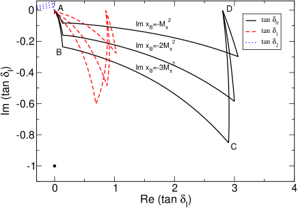
Figure B.1: Real and imaginary parts of $\tan\delta_{I}$ along the path ABCD, see Fig. 1. $x_{B}$ denote the imaginary part along the horizontal line BC. The black dot in the lower left corner denotes the position of the singularity $\tan\delta_{I}=-i$ (the $f_{0}(500)$ in the case of $I=0$ Caprini:2005zr ; Pelaez:2015qba ). It is seen that the singularity is never hit in the region spanned by the path ABCD with the choice (A) for the 4 vertices. Schenk parameterization Schenk:1991xe is used, with parameters from Colangelo:2001df , see appendix A.

Here, we wish to show that the original path of integration in (2) can be deformed into the lower complex $x$–plane. For this to achieve, we must prove that the integrand is holomorphic there. As an input, we need the phase shifts $\delta_{I}(x)$ and a starting value of the hat–functions $\hat{M}_{I}(x)$. For the latter, we use the current algebra expressions, which are polynomials in $x$ and thus even entire functions. Concerning the phase shifts, see appendix A. The Schenk parameterization used below 800 MeV has the virtue that the corresponding expression for the phase shift is holomorphic in a strip of the complex $x$–plane, cut for $x<4M_{\pi}^{2}$ and $x>700$ MeV. This is so because the Schenk parameterization provides a holomorphic expression for the tangent of the phase shifts. The phase shift itself is then obtained via

$$\delta_{I}(x)=\frac{1}{2i}\log{\frac{1+i\tan\delta_{I}(x)}{1-i\tan\delta_{I}(x)}}\,.$$ (B.1)

As long as $\tan\delta_{I}(x)\neq\pm i$, $\delta_{I}(x)$ is holomorphic. We display in Fig. B.1 the complex quantities $\tan\delta_{I}(x)$ along the polygonal path ABCD displayed in Fig. 1, and along similar paths which are nearer to the real line. It is seen that one does not hit any singularity. We have checked that the parameterization in terms of conformal variables as worked out in Ref. GarciaMartin:2011cn leads to the same conclusion.

We conclude that $\sin{\delta_{I}}$ is holomorphic in that region as well. Consider now the denominator of the measure, $|\Omega_{I}(x)|$. At first, it sounds surprising that one can continue analytically the modulus of a complex function. The point is that this quantity stands for

$$|\Omega_{I}(x)|=\exp\left(\frac{x}{\pi}-\int_{4M_{\pi}^{2}}^{\infty}\frac{dy}{y}\frac{\delta_{I}(y)}{y-x}\right),$$ (B.2)

where $-\int$ denotes a principal value integral. The relevant quantity is thus the integral

$$G_{I}(x)=\frac{x}{\pi}-\int_{4M_{\pi}^{2}}^{\infty}\frac{dy}{y}\frac{\delta_{I}(y)}{y-x}\,.$$ (B.3)

It is useful to first consider the related ordinary integral

$$H_{I}(x)=\frac{x}{\pi}\int_{4M_{\pi}^{2}}^{\infty}\frac{dy}{y}\frac{\delta_{I}(y)}{y-x}\,,\quad\quad x\in{\mathchoice{\hbox{\hbox to0.0pt{\kern 2.88884pt\vrule height=6.14993pt\hss}\hbox{$\displaystyle\sf C$}}}{\hbox{\hbox to0.0pt{\kern 2.88884pt\vrule height=6.14993pt\hss}\hbox{$\textstyle\sf C$}}}{\hbox{\hbox to0.0pt{\kern 2.02219pt\vrule height=4.30496pt\hss}\hbox{$\scriptstyle\sf C$}}}{\hbox{\hbox to0.0pt{\kern 1.44441pt\vrule height=3.07497pt\hss}\hbox{$\scriptscriptstyle\sf C$}}}}\,.$$ (B.4)

The function $H_{I}(x)$ is holomorphic in the complex $x$–plane, cut along the real axis for $x\geq 4M_{\pi}^{2}$. On the upper rim of the cut, $G_{I}$ and $H_{I}$ are closely related:

$$H_{I}(x+i0^{+})=i\delta_{I}(x)+G_{I}(x)\,,\quad x\in[4M_{\pi}^{2},\infty)\,.$$ (B.5)

Consider now the interval $[A,D]$ in Fig. 1. We can continue here $H_{I}(x)$ across the cut, because $\delta_{I}(x)$ are holomorphic there, and the integration path $\int_{A}^{D}$ can be deformed into the lower half plane, e.g., into the polygonal line ABCD in Fig. 1. The relation (B.5) shows that $G_{I}$ and thus $|\Omega(x)|$ can holomorphically be continued as well. The continuation is unique.

In practice, the continuation can be performed rather easily: One adds and subtracts the phase shift $\delta_{I}(x)$ in the integrand of $G_{I}(x)$ and obtains

$$G_{I}(x) = -\frac{\delta_{I}(x)}{\pi}\ln{\frac{x-4M_{\pi}^{2}}{4M_{\pi}^{2}}}$$ (B.6)

$$+ \frac{x}{\pi}\int_{4M_{\pi}^{2}}^{\infty}\frac{dy}{y}\frac{1}{y-x}[\delta_{I}(y)-\delta_{I}(x)]\,.$$

This identity holds for $x\in[4M_{\pi}^{2},\infty)$. In the integral on the right hand side, one need not use the principal value prescription. The right–hand side is holomorphic in the region where the phase shift is holomorphic.

Finally, the Omnès functions $\Omega_{I}(x)$ which enters the iterations in the region covered by the dashed-dotted blue lines in Fig. 6 may be evaluated in a manner analogous to $|\Omega_{I}(x)|$ just discussed: Below the threshold, use the integral representation (3), as well as above threshold, for Im$(x)>0$. In the case of Im$(x)\!<\!0$, Re$(x)\!>\!4M_{\pi}^{2}$, proceed as in the case of the principal value integral just discussed.

We conclude that we may indeed deform the path of integration as is indicated in the Fig. 1. [In order to render the proof watertight in view of the square–root singularities at the threshold $x=4M_{\pi}^{2}$, one may slightly change the paths. Let $A^{\prime}=4M_{\pi}^{2}+\epsilon,~{}\epsilon>0$. Then ABCDF$\to$ AA^′BCDF. Numerically, this change is irrelevant, and we stick to $\epsilon=0$.]

We have checked that the results do not change under a change of the polygonal line ABCD.

The following two remarks are in order at this place.

1. We do not assume that the phase shifts are holomorphic at all energies. As mentioned, we glue the phase shifts continuously together, using different parameterizations. Only in the low–energy region do we rely on a holomorphic parameterization.

2. One might argue that we extrapolate data from the real line to the polygonal line ABCD, which would be an unstable procedure. Instead, we make use of a holomorphic parameterization to render the integrations easier to perform. For a given parameterization, the result is the same, whether performed in the standard manner, or using a deformed path in the dispersion relation. The latter method is, however, by far more efficient.

Appendix C Allowed paths

Here, we discuss paths in the dispersive representation that allow for an undistorted path in the angular average, and follow the discussion in Aitchison:1966lpz . For fixed $x$, the angular average amounts to a line integral between $h_{\pm}(x)$. Starting from $x=\infty$ to lower values, it is clear from Fig. 2 that a critical value of $x$ is reached as soon as this straight line touches the value $4M_{\pi}^{2}$ for some $z\in[-1,1]$,

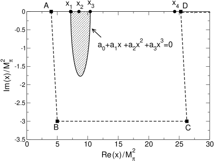
Figure C.1: Solid line: The part of the complex solutions of the polynomial equation (C.2) with Im ($x$)$<0$. Dashed: Deformed integration path used in the present work (displayed for $s\!<\!30M_{\pi}^{2}$). Any deformed path that does not cross the solid line allows for an undistorted integration in the angular average (4). See appendix A for the actual values chosen for $A,\ldots,D$ and for $x_{i}$.

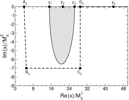
Figure C.2: The case $\omega\to 3\pi$. Solid line: Same as solid line in Fig C.1,with $M_{\eta}^{2}$ replaced by $M_{\omega}^{2}$. Dashed: A deformed integration path. Any deformed path that does not cross the solid line allows for an undistorted integration in the angular average (4). For notation see appendix A. Note that $\sqrt{D_{2}}\simeq 0.75$ GeV, i.e., the Schenk parameterization is still operative at $D_{2}$ and generates holomorphic phase shifts.

$$h(x,z)=4M_{\pi}^{2}\,.$$ (C.1)

This condition may be brought to the form

$$\sum_{i=0}^{3}a_{i}x^{i}=0\,,\,\,\quad\quad-1\leq z\leq 1\,,$$ (C.2)

with

$$a_{0} = -4z^{2}M_{\pi}^{2}(M_{\pi}^{2}-M_{\eta}^{2})^{2}\,,$$

$$a_{1} = z^{2}(3M_{\pi}^{2}+M_{\eta}^{2})^{2}-(M_{\eta}^{2}-5M_{\pi}^{2})^{2}\,,$$

$$a_{2} = -2z^{2}(M_{\eta}^{2}+3M_{\pi}^{2})+2M_{\eta}^{2}-10M_{\pi}^{2}\,,$$

$$a_{3} = z^{2}-1\,.$$ (C.3)

For a fixed value of $z\neq\pm 1$, the equation (C.2) has one real and 2 complex conjugate solutions for $x$. Varying $z$ in the interval $(-1,1)$ traces out 3 curves in the complex $x$–plane. The real branch (Im ($x$)=0) is located on the negative real axis, Re($x)\leq 0$. In Fig. C.1, we display the part of the complex solutions with Im$(x)<0$ (solid black line). If one uses a path in the dispersion integral that does not cross the hatched region, the angular average can be performed in the undeformed interval $-1\leq z\leq 1$. The polygonal line ABCDEF (displayed for $s<30M_{\pi}^{2}$) is the version used in the present work. See appendix A for the actual values chosen for $A,\ldots,F$ and for $x_{i}$.

The following two remarks are in order at this place.

• The reason to extend the polygonal line into the lower complex $x$–plane until $x=D$ is the following. After having solved the integral equation for the angular averages, one obtains the physical amplitudes by performing the final dispersive integration with Cauchy kernel $1/(x-s-i\epsilon)$. Even at $\epsilon=0$, this kernel is then not singular on the integration path for real values of $s$ with $s\not\in[D,F]$, except at the threshold $s=4M_{\pi}^{2}$. There, the integrand in (2) develops an integrable square root singularity in case of S-waves. It can be tamed with a transformation of variables, $z=A+(B-A)\tau^{2}\,,0\leq\tau\leq 1$. The integration can thus be performed at $\epsilon=0$, without further ado – an additional advantage of our procedure. For $s\in[D,F]$, due to the singularity of the Cauchy kernel, the angular average needs to be interpolated between the pertinent Gauss–Legendre points, before the integration can be done. This is the reason why we push $D$ to higher values than required.

• In order to stay away from the threshold region $x=4M_{\pi}^{2}$ while performing the angular average, we have chosen the path BC with an imaginary part that is more negative than what is needed according to the condition (C.2), see also Figs. 5 and 6.

Appendix D The decay $\omega\to 3\pi$

We shortly consider the situation for $\omega\to 3\pi$ decays Niecknig:2012sj . In Fig. C.2, we display the analogue to the boundary in Fig. C.1, for $M_{\eta}^{2}$ replaced by $M_{\omega}^{2}$. A possibility for the integration path is displayed with dashed lines. It is seen that with Schenk parameterization Schenk:1991xe , it is still possible to avoid the pseudothreshold singularity and to perform the dispersive integral without interpolation between Gauss–Legendre points in the interval $s<D_{2}$, which contains the decay region. We therefore expect that the method also works in this case.

References

- (1) N. N. Khuri and S. B. Treiman, Pion-Pion Scattering and K 3 Decay, Phys. Rev. 119 (1960) 1115.
- (2) V. N. Gribov, V. V. Anisovich and A. A. Anselm, Contribution to the theory of the and reactions near threshold, Sov. Phys. JETP 15 (1962) 159.
- (3) G. Bonnevay, A Model for Final-State Interactions, Nuov. Cim. 30 (1963) 1325.
- (4) J. B. Bronzan and C. Kacser, Khuri-Treiman Representation and Perturbation Theory, Phys. Rev. 132 (1963) 2703.
- (5) C. Kacser, Analytic Structure of Partial-Wave Amplitudes for Production and Decay Processes, Phys. Rev. 132 (1963) 2712.
- (6) J. B. Bronzan, Overlapping Resonances in Dispersion Theory, Phys. Rev. 134 (1964) B687.
- (7) I. J. R. Aitchison, Logarithmic Singularities in Processes with Two Final-State Interactions, Phys. Rev. 133 (1964) B1257.
- (8) I. J. R. Aitchison, Dispersion Theory Model of Three-Body Production and Decay Processes, Phys. Rev. 137 (1965) B1070.
- (9) R. Pasquier and J. Y. Pasquier, Khuri-Treiman-Type Equations for Three-Body Decay and Production Processes, Phys. Rev. 170 (1968) 1294.
- (10) R. Pasquier and J. Y. Pasquier, Khuri-Treiman-type equations for three-body decay and production processes. II, Phys. Rev. 177 (1969) 2482.
- (11) A. V. Anisovich, V. V. Anisovich, M. A. Matveev, V. A. Nikonov, J. Nyiri and A. V. Sarantsev, Three-particle physics and dispersion relation theory, World Scientific, Hackensack, USA, 2013.
- (12) A. V. Anisovich, Dispersion relation technique for three pion system and the -wave interaction in decay, Phys. Atom. Nucl. 58 (1995) 1383.
- (13) J. Kambor, C. Wiesendanger and D. Wyler, Final state interactions and Khuri-Treiman equations in decays, Nucl. Phys. B465 (1996) 215 [hep-ph/9509374].
- (14) A. V. Anisovich and H. Leutwyler, Dispersive analysis of the decay , Phys. Lett. B375 (1996) 335 [hep-ph/9601237].
- (15) M. Walker, , Master’s thesis, University of Bern, 1998.
- (16) H. Osborn and D. J. Wallace, mixing, and chiral lagrangians, Nucl. Phys. B20 (1970) 23.
- (17) J. Gasser and H. Leutwyler, to One Loop, Nucl. Phys. B250 (1985) 539.
- (18) I. J. R. Aitchison, Unitarity, Analyticity and Crossing Symmetry in Two- and Three-hadron Final State Interactions, arXiv:1507.02697 [arXiv:1507.02697].
- (19) G. Colangelo, J. Gasser and H. Leutwyler, scattering, Nucl. Phys. B603 (2001) 125 [hep-ph/0103088].
- (20) R. Kamiński, J. R. Peláez and F. J. Ynduráin, The Pion-pion scattering amplitude. III. Improving the analysis with forward dispersion relations and Roy equations, Phys. Rev. D77 (2008) 054015 [arXiv:0710.1150].
- (21) M. Bissegger, A. Fuhrer, J. Gasser, B. Kubis and A. Rusetsky, Radiative corrections in decays, Nucl. Phys. B806 (2009) 178 [arXiv:0807.0515].
- (22) C. Ditsche, B. Kubis and U.-G. Meißner, Electromagnetic corrections in decays, Eur. Phys. J. C60 (2009) 83 [arXiv:0812.0344].
- (23) KLOE collaboration, F. Ambrosino et al., Determination of Dalitz plot slopes and asymmetries with the KLOE detector, JHEP 05 (2008) 006 [arXiv:0801.2642].
- (24) Crystal Ball at MAMI, A2 collaboration, S. Prakhov et al., Measurement of the Slope Parameter alpha for the decay with the Crystal Ball at MAMI-C, Phys. Rev. C79 (2009) 035204 [arXiv:0812.1999].
- (25) Crystal Ball at MAMI, TAPS, A2 collaboration, M. Unverzagt et al., Determination of the Dalitz plot parameter alpha for the decay with the Crystal Ball at MAMI-B, Eur. Phys. J. A39 (2009) 169 [arXiv:0812.3324].
- (26) KLOE collaboration, F. Ambrosino et al., Measurement of the slope parameter with the KLOE detector, Phys. Lett. B694 (2011) 16 [arXiv:1004.1319].
- (27) WASA-at-COSY collaboration, P. Adlarson et al., Measurement of the Dalitz plot distribution, Phys. Rev. C90 (2014) 045207 [arXiv:1406.2505].
- (28) BESIII collaboration, M. Ablikim et al., Measurement of the Matrix Elements for the Decays and , Phys. Rev. D92 (2015) 012014 [arXiv:1506.05360].
- (29) KLOE-2 collaboration, A. Anastasi et al., Precision measurement of the Dalitz plot distribution with the KLOE detector, JHEP 05 (2016) 019 [arXiv:1601.06985].
- (30) A2 collaboration, S. Prakhov et al., High-statistics measurement of the decay at the Mainz Microtron, Phys. Rev. C97 (2018) 065203 [arXiv:1803.02502].
- (31) S. Lanz, Determination of the quark mass ratio from , Ph.D. thesis, University of Bern, 2011.
- (32) G. Colangelo, S. Lanz, H. Leutwyler and E. Passemar, Determination of the light quark masses from , PoS EPS-HEP2011 (2011) 304.
- (33) S. Lanz, and quark masses, PoS CD12 (2013) 007 [arXiv:1301.7282].
- (34) S. Descotes-Genon, E. Kou and B. Moussallam, Dispersive evaluation of the second-class amplitude in the standard model, Nucl. Phys. Proc. Suppl. 253-255 (2014) 65 [arXiv:1303.2879].
- (35) S. Descotes-Genon and B. Moussallam, Analyticity of isospin-violating form factors and the second-class decay, Eur. Phys. J. C74 (2014) 2946 [arXiv:1404.0251].
- (36) P. Guo, I. V. Danilkin, D. Schott, C. Fernández-Ramírez, V. Mathieu and A. P. Szczepaniak, Three-body final state interaction in , Phys. Rev. D92 (2015) 054016 [arXiv:1505.01715].
- (37) B. Moussalam and M. Albaladejo, mixing in the Khuri-Treiman equations for , PoS CD15 (2015) 057 [arXiv:1510.06626].
- (38) B. Moussallam and M. Albaladejo, Role of the resonances in from the Khuri-Treiman formalism, EPJ Web Conf. 130 (2016) 03007.
- (39) P. Guo, I. V. Danilkin, C. Fernández-Ramírez, V. Mathieu and A. P. Szczepaniak, Three-body final state interaction in updated, Phys. Lett. B771 (2017) 497 [arXiv:1608.01447].
- (40) G. Colangelo, S. Lanz, H. Leutwyler and E. Passemar, : Study of the Dalitz plot and extraction of the quark mass ratio , Phys. Rev. Lett. 118 (2017) 022001 [arXiv:1610.03494].
- (41) M. Albaladejo and B. Moussallam, Extended chiral Khuri-Treiman formalism for and the role of the , resonances, Eur. Phys. J. C77 (2017) 508 [arXiv:1702.04931].
- (42) G. Colangelo, S. Lanz, H. Leutwyler and E. Passemar, Dispersive analysis of , Eur. Phys. J. C78 (2018) 947 [arXiv:1807.11937].
- (43) F. Niecknig, B. Kubis and S. P. Schneider, Dispersive analysis of and decays, Eur. Phys. J. C72 (2012) 2014 [arXiv:1203.2501].
- (44) F. Niecknig and B. Kubis, Dispersion-theoretical analysis of the Dalitz plot, JHEP 10 (2015) 142 [arXiv:1509.03188].
- (45) F. Niecknig, Dispersive analysis of charmed meson decays, Ph.D. thesis, Bonn U., HISKP, 2016.
- (46) T. Isken, B. Kubis, S. P. Schneider and P. Stoffer, Dispersion relations for , Eur. Phys. J. C77 (2017) 489 [arXiv:1705.04339].
- (47) F. Niecknig and B. Kubis, Consistent Dalitz plot analysis of Cabibbo-favored decays, Phys. Lett. B780 (2018) 471 [arXiv:1708.00446].
- (48) C. Roiesnel and T. N. Truong, Resolution of the Problem, Nucl. Phys. B187 (1981) 293.
- (49) J. Bijnens and J. Gasser, decays at and beyond in chiral perturbation theory, Phys. Scripta T99 (2002) 34 [hep-ph/0202242].
- (50) J. Bijnens and K. Ghorbani, at Two Loops In Chiral Perturbation Theory, JHEP 11 (2007) 030 [arXiv:0709.0230].
- (51) S. P. Schneider, B. Kubis and C. Ditsche, Rescattering effects in decays, JHEP 02 (2011) 028 [arXiv:1010.3946].
- (52) S. P. Schneider, Analysis tools for precision studies of hadronic three-body decays and transition form factors, Ph.D. thesis, University of Bonn, 2013.
- (53) P. Guo, Analytic continuation of the Pasquier inversion representation of the Khuri-Treiman equation, Phys. Rev. D91 (2015) 076012 [arXiv:1412.3970].
- (54) P. Guo, I. V. Danilkin and A. P. Szczepaniak, Dispersive approaches for three-particle final state interaction, Eur. Phys. J. A51 (2015) 135 [arXiv:1409.8652].
- (55) I. J. R. Aitchison and R. Pasquier, Three-Body Unitarity and Khuri-Treiman Amplitudes, Phys. Rev. 152 (1966) 1274.
- (56) J. Hadamard, Théorème sur les séries entières, Acta Math 22 (1898) 55.
- (57) R. J. Eden, Threshold behaviour in quantum field theory, Proc. Roy. Soc. A 210 (1952) 388.
- (58) R. J. Eden, P. V. Landshoff, D. I. Olive and J. C. Polkinghorne, The Analytic S-Matrix, Cambridge University Press, 1966.
- (59) J. H. Hetherington and L. H. Schick, Exact Multiple-Scattering Analysis of Low-Energy Elastic Scattering with Separable Potentials, Phys. Rev. 137 (1965) B935.
- (60) E. W. Schmid and H. Ziegelmann, Quantum Mechanical Three-body Problem, Pergamon Press, 1974.
- (61) D. E. Soper, QCD calculations by numerical integration, Phys. Rev. Lett. 81 (1998) 2638 [hep-ph/9804454].
- (62) Z. Nagy and D. E. Soper, Numerical integration of one-loop Feynman diagrams for N-photon amplitudes, Phys. Rev. D74 (2006) 093006 [hep-ph/0610028].
- (63) B. Kubis, private communication.
- (64) The NAG Fortran Library, the Numerical Algorithms Group (NAG), Oxford, United Kingdom, www.nag.com.
- (65) S. Lanz, private communication.
- (66) A. Schenk, Absorption and dispersion of pions at finite temperature, Nucl. Phys. B363 (1991) 97.
- (67) I. Caprini, G. Colangelo and H. Leutwyler, Mass and width of the lowest resonance in QCD, Phys. Rev. Lett. 96 (2006) 132001 [hep-ph/0512364].
- (68) J. R. Peláez, From controversy to precision on the sigma meson: a review on the status of the non-ordinary resonance, Phys. Rept. 658 (2016) 1 [arXiv:1510.00653].
- (69) R. García-Martín, R. Kamiński, J. R. Peláez, J. Ruiz de Elvira and F. J. Ynduráin, The Pion-pion scattering amplitude. IV: Improved analysis with once subtracted Roy-like equations up to 1100 MeV, Phys. Rev. D83 (2011) 074004 [arXiv:1102.2183].