Déjà Vu: an empirical evaluation of the memorization properties of ConvNets

Abstract

Convolutional neural networks memorize part of their training data, which is why strategies such as data augmentation and drop-out are employed to mitigate overfitting. This paper considers the related question of “membership inference”, where the goal is to determine if an image was used during training. We consider it under three complementary angles. We show how to detect which dataset was used to train a model, and in particular whether some validation images were used at train time. We then analyze explicit memorization and extend classical random label experiments to the problem of learning a model that predicts if an image belongs to an arbitrary set. Finally, we propose a new approach to infer membership when a few of the top layers are not available or have been fine-tuned, and show that lower layers still carry information about the training samples. To support our findings, we conduct large-scale experiments on Imagenet and subsets of YFCC-100M with modern architectures such as VGG and Resnet.

1 Introduction

The widespread adoption of convolutional neural networks (LeCun et al., 1990) (ConvNets) for most recognition tasks, was triggered by the advance of Krizhevsky et al. (2012) in image classification and subsequent deep architectures (Simonyan & Zisserman, 2014; He et al., 2016). Several works have analyzed these architectures from different perspectives. Zeiler & Fergus (2014) have proposed DeconvNet to vizualize filter activations. Lenc & Vedaldi (2015) analyze their equivariance. Mahendran & Vedaldi (2015) show how to invert them and synthetize images maximizing the response of different classes. Ulyanov et al. (2017) analyze the image priors implicitly defined by ConvNets.

All these works increase our understanding of ConvNets, but the complex issue of overfitting and its relationship to optimization are still not fully understood. Several strategies are routinely used to avoid overfitting, such as $\ell_{2}$-regularization through weight decay (Krogh & Hertz, 1991), dropout (Srivastava et al., 2014), and importantly, data augmentation (Behpour et al., 2017; Dwibedi et al., 2017; Paulin et al., 2014). Yet few works (Zhang et al., 2016; Yeom et al., 2018) have analyzed the interplay of overfitting and memorization of training images in high-capacity classification architectures. Specifically, we are not aware of such an analysis for a modern ConvNet such as ResNet-101 learned on Imagenet.

In this paper, we consider the privacy issue of membership inference, i.e., we aim at determining if a specific image or group of images was used to train a model. This question is important to protect both the privacy and intellectual property associated with images. For ConvNets, the privacy issue was recently considered by Yeom et al. (2018) for the small MNIST and CIFAR datasets. The authors evidence the close relationship between overfitting and privacy of training images. This is reminiscent of prior membership inference attacks, which employ the output of the classifier associated with a particular example to determine whether it was used during training or not (Shokri et al., 2016). This is related to Torralba & Efros (2011), who showed that a classifier can determine with high accuracy if an image comes from a dataset or another by exploiting the bias inherent to datasets. We discuss this relationship and show that we can detect whether a given network has been trained on some of the validation images. This has a concrete application for machine-learning benchmarks: scores are often reported on a validation set with public labels, allowing a malicious or gawky competitor to artificially inflate the accuracy by training on validation images. Our test detects if it is the case, even if only part of the validation set is leaked to the training set.

We provide a qualitative upper bound on the capacity of popular convolutional networks to memorize a given number of images. More precisely, we construct a binary classifier as a drop-in replacement of the last layer, whose response is the membership test. Our tests carried out on VGG-16 (Simonyan & Zisserman, 2014) and ResNet-101 (He et al., 2016) evidence different memorizing capabilities depending on the number of images and the amount of data augmentation (flip, cropping).

Finally, we propose a new setting for membership inference that only considers intermediary layers of a network, thus extending membership inference to transferred and fine-tuned networks, that have become ubiquitous. Our membership inference does not require the last layer(s) of the original ConvNet to perform the test. This is important because, in many contexts, image recognition systems are built upon a trunk trained on a dataset and then fine-tuned for another task. Examples include Mask-RCNN (He et al., 2017) and models used for fine-grained recognition (Hariharan & Girshick, 2017). In both cases there are not enough training samples to train a full network: only the last layers of the networks are fine-tuned. In summary, our paper makes the following contributions:

• A simple statistical test to detect the “signature” of a dataset in a trained convnet, and to detect if validation images where used to train the model (leakage).

• An empirical analysis of the explicit memorization capabilities of the ResNet and VGG architectures at a much larger scale than previously reported. We evaluate the factors impacting the memorization capabilities such as the number of images “stored” in the network and the equivariance hypotheses in data augmentation.

• A membership inference test that detects if an image was used to train the trunk of a network. To our knowledge, it is the first work on membership inference that attacks intermediate layers.

The paper is organized as follows. Section 2 reviews related work. Section 3 evaluates the capacity of ConvNets to memorize a given set of images. Section 4 considers the problem of determining if a particular dataset, e.g., the validation set, was used during training. Section 5 focuses on detecting if a particular image has been used for training without accessing the network’s output layer.

2 Related work & datasets

Our work is related to the topics of overfitting and memorization capabilities of neural network architectures, which are able to perfectly discriminate random outputs in some cases (MacKay, 2002; Zhang et al., 2016). In the following, we distinguish explicit from implicit memorization (also called “unintended memorization” (Carlini et al., 2018) in natural language processing systems).

Explicit memorization.   Neural network are capable of memorizing any random pattern. This property was analyzed in MacKay (2002) for the single layer case. In MacKay’s setup, the sender and receiver agree beforehand on a set of vectors $(x_{i})_{i=1}^{n}\in\mathbb{R}^{d}$. To transmit an arbitrary sequence of binary labels $y_{1},\dots,y_{n}$, the sender learns a single-layer neural network that predicts the $y_{i}$ from $x_{i}$, and sends its weights to the receiver. The receiver labels the points $x_{1},\dots,x_{n}$ with the transmitted neural network to reconstruct the labels. The VC-dimension of this 1-layer model is $d$, so the model can fit perfectly as long as $n\leq d$. MacKay extends this bound by showing that the sender can, with high probability, find a neural network fitting the output if $n\leq 2d$, and that it is almost impossible to fit the model for $n>2d$. The estimated capacity of this neural network is thus $2$ bits per parameter.

Determining the practical memorization capacity of ConvNets is not trivial. A few recent works (Zhang et al., 2016; Yeom et al., 2018) evaluate how a network can fit random labels. Zhang et al. (2016) replace true labels by random labels and show that popular ConvNets can perfectly fit them in simple cases, such as small datasets (CIFAR10) or Imagenet without data augmentation. Krueger et al. (2017) extend their analysis and argue in particular that the effective capacity of ConvNets depends on the dataset considered. In a privacy context, Yeom et al. (2018) exploit this memorizing property to watermark networks. As a side note, random labeling and data augmentation have been used for the purpose of training a network without any annotated data (Dosovitskiy et al., 2014; Bojanowski & Joulin, 2017). Our paper is also related to few works (Kraska et al., 2017; Iscen et al., 2017) that learn indexes as an alternative to traditional structures such as Bloom Filters or B-trees. In particular, Kraska et al. (2017) show that in some cases, neural nets outperform cache-optimized B-tree on real-world data. These works exploiting explicit memorization of neural networks are reminiscent of works (Hopfield, 1982; Personnaz et al., 1986; Hinton et al., 1986; Plate, 1995) on associative memories and, more generally, distributed representations.

Implicit memorization and privacy risk in learning systems.   Ateniese et al. (2015) state: “it is unsafe to release trained classifiers since valuable information about the training set can be extracted from them”. The problem that we address in this paper, i.e., to determine whether an image or dataset has been used for training, is related to the privacy implications of machine learning systems. They were discussed in the context of support vector machines (Rubinstein et al., 2009; Biggio et al., 2014). In the context of differential privacy (Dwork et al., 2006), recent works (Wang et al., 2016; Bassily et al., 2016) suggest that guaranteeing privacy requires learning systems to generalize well, i.e., to not overfit. Note that there are systems providing differential privacy but that still leak information (Ateniese et al., 2015; Balu et al., 2014).

Membership Inference in images.   A few recent works (Abadi et al., 2016; Hayes et al., 2017; Shokri et al., 2016; Long et al., 2018) have addressed “membership inference” for images: determine whether an image has been used for training or not. Yeom et al. (2018) discuss how privacy, that can be broken by membership inference, is connected to overfitting. Long et al. (2018) observe that some training images are more vulnerable than others and propose a strategy to identify them. Hayes et al. (2017) analyze privacy issues arising in generative models. Most of these works were evaluated on small datasets like CIFAR10, or larger datasets but without data augmentation. Our work aims at being closer to realistic conditions. In the following, the analysis of a pre-trained network will be called “attack” performed by an “attacker”.

Dataset bias and inference.   Torralba & Efros (2011) evidence that a simple classifier can predict with high accuracy which dataset an image comes from. Tommasi et al. (2017) show that this bias still exists with ConvNets. In the next section of this paper, we re-visit this problem by proposing a dataset inference method derived from an elementary membership inference test.

Datasets used in our study.   We use will several public image collections throughout our paper. Imnet1k refers to the subset of Imagenet (Deng et al., 2009; Russakovsky et al., 2015) used during the ILSVRC-12 challenge. It consists of 1000 balanced classes, split in a training set (1.2M images) and a validation set (50k images). We use the regular split between train and val and denote them by Imnet1k-train and Imnet1k-val, respectively. Imnet22k refers to the full Imagenet dataset. It is built in the same way as Imnet1k, but with 21783 unbalanced classes. Yfcc100M (Thomee et al., 2016) contains 99.2M photos that have not been collected for image classification and thus are not representing specific classes or visual concepts. Tiny images  (Torralba et al., 2008) consists of 79M low-resolution images. CIFAR10 is a subset of Tiny that has been labelled for image classification. In our study, it is important that the dataset does not contain duplicate images or images that overlap between the train and the test set. We have sanitized the datasets to avoid this problem using GIST descriptors and similarity search, see Appendix B in the supplemental material for details.

3 Explicit memorization – network capacity

In this section, we explicitly train neural networks to memorize a given subset of images, so that it can decide whether an image is in its memory or not at test time. We design a model $f_{\theta}$ that distinguishes a set of in images from out images, where images unseen during training are out.

We repurpose the classification layer of standard models to output a binary label, depending on whether the image must be remembered or not. Our architecture plays an equivalent role to the discriminator in Generative Adversarial Networks (GAN): it needs to discriminate between positive and negative images. In our case, negative images are a large pool of images instead of the generated images in GANs. Zhang et al. (2016) show that ConvNets are able to overfit almost any random labelling of their input data, but in their experiment, the output for unseen images is undefined.

3.1 Information-theoretic capacity

We train our model to predict $1$ for a set of positive images $\mathcal{P}$, and $0$ for all other (negative) images $\mathcal{N}$. We assume that $\mathcal{N}$ represent a large image distribution, so $n=|\mathcal{P}|\ll|\mathcal{N}|$, and we note $N=|\mathcal{P}|+|\mathcal{N}|$. There are two notions of capacity relevant to our analysis: the capacity of a neural network, and the capacity needed to store a number $n$ of images among a larger set of size $N$. We assume, following MacKay’s analysis, that the capacity of a neural network is well approximated by its number of parameters. Assuming images have consecutive ids, it is sufficient to store the subset of ids of the positive images, which requires a capacity:

$$C(n)=\log_{2}{N\choose n}\approx n\log_{2}\left(\frac{N}{n}\right)+\frac{n}{\log(2)},$$ (1)

where the approximation holds for $n\ll N$. This number scales almost linearly in the number of positive examples $n$, and logarithmically in the number of negatives.

3.2 Empirical analysis on tiny images

TinyNet.   We design a family of ConvNets with 4 convolutional layers and 2 fully-connected layers that take 32x32 images as input and output a binary classification. There are 3 versions: TinyNet-1, (90k parameters), TinyNet-2 (300k parameters) and TinyNet-3 (2M parameters). Most parameters of these models are in the first fully connected layer, as in VGG (cf. Appendix C).

Experimental setup.   We use a subset of $N=15M$ images from Tiny for these experiments. We randomly sample $n$ images as positive examples, and treat the rest as negatives. At each epoch, we feed a random sample of negatives of the same size as the number of positives to the network. The reported accuracy is measured on a balanced set of positives and negatives. We consider four types of data augmentation: “none”, “flip” (random horizontal mirroring), “flip+crop$\pm$1” (a random translation in $\{-1,0,+1\}^{2}$), “flip+crop$\pm$2”.

TinyNet-1	TinyNet-2	TinyNet-3

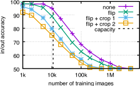
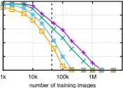
Figure 1: In/out classification performance (train) on Tiny, for varying image subsets and number of images. The colors indicate the type of data augmentation: purple=none, green=flip, cyan=flip+crop$\pm$1, orange=flip+crop$\pm$2. The vertical line shows the number of positive images $n$ such that $C(n)$ is the number of parameters of the network.

Discussion.   Figure 1 shows the accuracy of the model as a function of the number of positive images for all TinyNets. Instead of a sharp drop between the over-capacity and the under-capacity regimes, we observe a smooth drop as the number of positives increases. Empirically, this transition phase happens when the number of samples reaches the theoretical capacity of the network.

As expected, data augmentation reduces the memorization capacity of the network. For example, the accuracy of a network trained on $n$ images with flips is lower-bounded by the capacity of the same network trained on $2n$ images with no data augmentation. This lower bound is not tight, thanks to the generalization capability of the ConvNet, which captures the patterns common to an image and its symmetric. This generalization capability is obvious for stronger augmentations: for example with “flip+crop$\pm$1” TinyNet-2 can identify 10k images with 90% accuracy, vs. 20k images without data augmentation, while this requires to treat 18 augmented versions of each image similarly.

3.3 Experiments with large-scale architectures

In this section, we extend the explicit memorization experiments to VGG-16, ResNet-18, and ResNet-101 networks with images coming from Yfcc100M. The capacity of these networks is much larger than in the tiny setting: Resnet-18 has 11.7M parameters and VGG-16 has 140M.

We set an initial learning rate of $10^{-2}$ and divide it by $10$ when the accuracy gets over 60%, and again at 90%. We run experiments using either the center crop, or two data augmentations (flip, flip+crop$\pm 5$). Figure 2 shows convergence plots for several settings. Note, the x-axis is in epochs, that are 10$\times$ slower for $n=$100k images than $n=$10k images. The longest experiment took 4 days on 4 GPUs . VGG-16 and ResNet-101 converge at approximately the same number of epochs, irrespective of $n$. Data augmentation increases the number of epochs required to converge, eg. for the ResNets, flip up to twice more epochs to be trained. VGG is a more shallow and higher capacity network; in general it converges faster and it handles crops better than the ResNet variants.

	resnet-18	resnet-101	VGG-16
$n$=10k
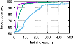
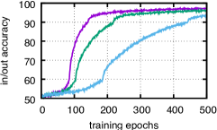
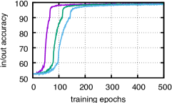
$n$=100k

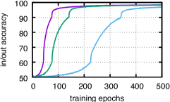
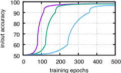
Figure 2: Accuracy over iterations of the in/out training on Yfcc100M for different networks and amount of data augmentation (indicated by color: purple= none, green = flip, cyan = flip+crop$\pm$5).

The outcome of our analysis is that explicit memorization of a large amount of images is possible, albeit more difficult with data augmentation. In real use cases, the number of images that can be stored explicitly with perfect accuracy is practically much lower than the number of network parameters. This set of experiments provides an approximate upper-bound for the problem of membership inference: if a given model cannot perfectly remember a set of images when trained to do so, it will likely not be able to remember all the images of the training set when trained for classification.

4 Dataset detection and leakage

In this section, we detect whether a group of samples or a dataset has been used to train a model. This problem encompasses the particular case of dataset bias (Torralba & Efros, 2011) and is more difficult, as we need to distinguish datasets even if they share the same statistics, acquisition procedure and labelling process. For instance, we want to be able to determine if images from the validation set of Imnet1k were used at train time.

Hypothesis and problem statement.   We assume that there are two data sources $S_{1},S_{2}$ and each source $S_{j}$ yields samples $x_{1}^{(j)},x_{2}^{(j)},\dots,x_{m}^{(j)}$. The attacker is given access to a model $f_{\theta}$; in this paper, we assume $f_{\theta}(x)$ is the maximal activation of the softmax layer, aka. the confidence of the model. The cumulative distribution of the confidence for a model trained on Imnet1k-train is shown in figure 3: most samples coming from the source Imnet1k-train have a very high confidence, while the distribution of the source Imnet1k-val is more balanced and unrelated sources (Yfcc100M, Imnet22k) tend to have a more uniform distribution.

We consider two attack scenarii on the model $f_{\theta}$. In the first scenario, we have a set of $m$ samples that come from either $S_{1}$ or $S_{2}$ and we want to determine which source they come from. In the second scenario, we want to determine if the model has been trained with samples from a validation set, and thus look at whether the two source distributions corresponding to the validation and the test are different.

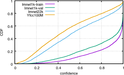
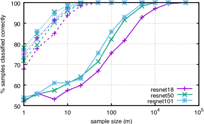
Figure 3: Left: Cumulative distribution of the maximum classification score for a sample of 5000 images taken from 4 datasets. Imnet1k-train served as the training set and therefore Imnet1k images (both train and val) have higher confidence. Right: binary classification accuracy (%) of a sample of $m$ elements from the training set Imnet1k-train w.r.t. three other datasets: Imnet1k-val (solid), Imnet22k (dashed) and Yfcc100M (lines). The architecture is indicated by the line color.

We compare confidence distributions using the Kolmogorov-Smirnov (K-S) distance. Given two cumulative distributions $F$ and $G$, the K-S distance is $d_{\text{KS}}(F,G)=\sup_{x}|F(x)-G(x)|.$ We use the K-S distance to determine if two distributions are similar.

4.1 Confidence as a signature of a dataset

In this section the samples $x_{1},\dots,x_{m}$ come from either source $S_{1}$ or $S_{2}$. The attacker uses the following decision rule: compute the K-S distance between $x_{1},\dots,x_{m}$ and $S_{1}$ (resp. $S_{2}$), and assign the samples to the closest source.

Results and observations.   The results are reported in Figure 3. We can distinguish Imnet1k-train from Yfcc100M with very few (10-20) samples. More interestingly, the same number of samples allow us to separate Imnet22k from Imnet1k-train, and with 500 images we can distinguish Imnet1k-train from Imnet1k-val. This shows that, even with a relatively low number of images, an attacker can determine that a given image collection was used for training. The figure also shows that the test is easier for networks with a higher capacity, that tend to overfit more.

4.2 Detecting leakage

We now assume that we are given a model for which we suspect that part of the validation set was used for training (leakage). For a number of datasets (e.g., Imagenet, Pascal VOC), the labels of the validation set are publicly available, and models are often compared using validation accuracy. A malicious person could train a model using the training set and part of the validation set, and then report validation accuracy to artificially inflate the performance of the model.

The attack we propose is a two-sample K-S test to determine if leakage has occurred or not. We assume that no sample from the test set has leaked (labels are not public in most cases). The null hypothesis of our test is that the validation and test sets have the same distribution. We compute the K-S distance between the validation and test sets, and reject the null hypothesis if this distance is high. The distance threshold $t$ is set such that the null hypothesis is incorrectly rejected with a low probability $\alpha$, corresponding to the $p$-value. For large samples, Smirnov’s estimate of the threshold corresponding to a $p$-value of $\alpha$ is (Feller, 1949):

$$t=c(\alpha)\sqrt{\frac{n+m}{nm}}\textrm{\ \ \ where\ \ \ }c(\alpha)=\sqrt{-\frac{1}{2}\log\left(\frac{\alpha}{2}\right)}.$$ (2)

We ran experiments on Imagenet using Resnet-18 and VGG-16, with $s\in\{1,2,5,10,20\}$ images per class of the validation set in addition to the training set to fit the model. Table 1 reports the $p$-value of the different tests. We can see that when $10$ images per class are leaked, the K-S test predicts that leakage has happened with a very high significance. When $5$ images per class or less are used, we cannot reject the null hypothesis and thus cannot claim that leakage has happened.

Table 1: Kolmogorov-Smirnov tests on Imnet1k validation and test sets for various levels of leakage. The K-S test provides a level of significance ($p$-value) rather than a yes/no answer. Lower values indicate high confidence that the validation and test sets distributions are different, hinting that leakage has occurred. If only $1$ image per class of the validation set has leaked, we cannot conclude from this test that there has been leakage. Conversely, when $10$ images or more have leaked, we can conclude with high significance that leakage has occurred.

Nb. of Images
# per class leaked	Resnet-18	VGG-16
1	$0.888$	$0.494$
2	$0.228$	$0.107$
5	$0.068$	$0.014$
10	$<10^{-4}$	$<10^{-4}$
20	$<10^{-4}$	$<10^{-4}$

5 Implicit memorization & membership inference

This section tackles the more difficult problem of membership inference in trained models. From a trained model and an image the attacker has to determine whether the image was used to train the model. In our new setting, upper layers are not available (due to e.g. finetuning on a downstream task). We provide baselines for VGG16 and Resnet and extend the traditional attacks to our setup.

The literature (Abadi et al., 2017) distinguishes two cases types of membership inference: (1) all layers are available (all-layers), (2) only the final output of the network is available (final-output). There is currently no attack that performs substantially better in all-layers than in final-output. This seems counter-intuitive but we confirmed it in preliminary experiments. Our new setup, partial-layers, is adapted to transfer learning: only a certain number of bottom layers are available for attack, the remaining layers were destroyed by retraining on an unrelated task. This task is more difficult than all-layers since it has less parameters available, and thus more difficult than final-output.

5.1 Evaluation protocol and baselines

We assume that there are three disjoint sources of data: a public set, a private set, and an evaluation set. A model is trained on the private set. The attacker has access to the lower layers of this model and to the public set. After the attack is carried out, the evaluation is ran on images from the private and evaluation sets.

We divide Imnet1k equally into two splits (each with half of the images per class). We hold out $50$ images per class in the first split to form the evaluation set, and form the private set with the rest of this split. The second split is used as the public dataset. We conduct the membership inference test by comparing the prediction of the attack model on the private set and on the evaluation set. For this purpose, we consider the two baseline methods.

Bayes rule.   A simplistic membership inference attack is to predict that an image comes from the training set if its class is predicted correctly, and from a held-out set otherwise. We note $p_{\text{train}}$ (resp. $p_{\text{test}}$) the classification accuracy on the training (resp. held-out) set, and assume a balanced prior on membership. According to Bayes’ rule, the accuracy of the heuristic is (see Appendix A in the supplementary material for the derivation):

$$p_{\text{bayes}}=1/2+(p_{\text{train}}-p_{\text{test}})/2.$$ (3)

Since $p_{\text{train}}\geq p_{\text{test}}$ this heuristic is better than random guessing (accuracy $1/2$) and the improvement is proportional to the overfitting gap $p_{\text{train}}-p_{\text{test}}$.

Maximum Accuracy Threshold (MAT).   Yeom et al. (2018) propose an attack on the loss value: a sample is deemed part of the training set if its loss is below a threshold $\tau$. If $F_{\text{train}}$ (resp. $F_{\text{heldout}}$) is the cdf of the loss on the train (resp. held out), the accuracy of the MAT is:

$$p_{\text{threshold}}=\max_{\tau}~{}1/2+1/2\left(F_{\text{train}}(\tau)-F_{\text{heldout}}(\tau)\right)$$ (4)

As $F_{\text{train}}(\tau)\geq F_{\text{heldout}}(\tau)$, this heuristic is also better than random guessing. In practice, $\tau$ is estimated with samples or simulated by training models with known train/heldout split.

5.2 Membership inference with a truncated network

In this section, we provide a simple method to attack networks in the partial-layers setting. We use the available public data to retrain the missing layers, and apply either the Bayes or the MAT attack, as if there was no fine-tuning at all. We found this method to be more accurate than another variant that we designed with shadow models (Shokri et al., 2016), as detailed in the supplemental material (Appendix E).

Table 2: Accuracy of membership inference attacks on the softmax layer of the models (final-output). Data augmentation reduces the gap between the training accuracy and the held-out accuracy, thus decreasing the accuracy of the Bayes attack and the MAT attack.

Model	Augmentation	Bayes baseline	MAT
Resnet101	None	76.3	90.4
	Flip, Crop $\pm 5$	69.5	77.4
	Flip, Crop	65.4	68.0
VGG16	None	77.4	90.8
	Flip, Crop $\pm 5$	71.3	79.5
	Flip, Crop	63.8	64.3

5.3 Experiments on large convnets

Classification models.   We experiment with the popular VGG-16 (Simonyan & Zisserman, 2014) and Resnet-101 (He et al., 2016) architectures. The private model is learned in $90$ epochs, with an initial learning rate of $0.01$, divided by $10$ every $30$ epochs. Parameter optimization is conducted with stochastic gradient descent with a momentum of $0.9$, a weight decay of $10^{-4}$, and a batch size of $256$. To assess the effect of data augmentation, we train different networks with varying data augmentation: flip+crop$\pm$5, flip+crop, flip+crop+resize, or none.

Attack models.   We evaluate both the bayes and MAT methods to estimate the performance on final-output. The results are shown in Table 2. As we can see, it is possible to guess with a very high accuracy if a given image was used to train a model when there is no data augmentation. Stronger data augmentation reduces the accuracy of the attacks, that still remain above $64\%$.

The results of our attack in the more challenging partial-layers setting are shown in Table 3. We can see that even without the last layers, it is possible to infer training set membership of an image. The attack performance depends on two factors: the layer at which the attack is conducted, and the data augmentation used to train the original network. As expected, it is more difficult to attack a network that has been trained with more data augmentation, or that has only lower layers available. More importantly, these experiments show that intermediary layers still carry out information about the images used for training the model.

Table 3: Accuracy of membership inference attacks on intermediate layers of Resnet-101 and VGG-16 models (partial-layers).
Last block corresponds to the softmax, and respectively the fully connected layers (for VGG-16) and the 4-th stage of Resnet (for Resnet-101).

Augmentation	Truncate	Resnet-101	VGG-16
None	Softmax	73.4	74.8
	Last block	53.1	51.7
Flip, Crop$\pm 5$	Softmax	65.7	67.3
	Last block	53.1	52.2
Flip, Crop	Softmax	60.8	58.5
	Last block	52.9	53.2

6 Conclusion

We have investigated the memorization capabilities of neural networks from different perspectives. Our experiments show that state-of-the-art networks can remember a large number of images and distinguish them from unseen images. We have analyzed networks specifically trained to remember a set of images and the factors influencing their memorizing and convergence capabilities. It is possible to determine whether an image set was used at training time, even with full data augmentation. On the contrary, the accuracy of determining if a single image was used is low when considering full data augmentation on a large training set such as Imagenet. This implies that data augmentation is an effective privacy-preserving method. Our last contribution is a method that detects training images better than chance even with no access to the last layers, under limited data augmentation.

Final remark:   The curious reader may have noticed that our title echoes the one of a previous user study (Dhamija et al., 2000), in which the authors discussed the feasibility of authenticating humans by their capabilities to recognize a set of images.

Appendix A Probabilistic derivations

A.1 Bayes attack

Let $C$ denote the event that the prediction of the neural network is correct and $S$ the random variable that indicates whether the sample comes from the training set. We therefore have:

$$\mathbb{P}(C=1|S=1)=p_{\text{train}}, ~{}\mathbb{P}(C=1|S=0)=p_{\text{test}}$$ (5)

$$\mathbb{P}(S=1)= \mathbb{P}(S=0)=1/2.$$ (6)

The accuracy of Bayes attack is:

$$\mathbb{P}(C=S) =\mathbb{P}(C=1~{}|~{}S=1)\mathbb{P}(S=1)$$ (7)

$$+\mathbb{P}(C=0~{}|~{}S=0)\mathbb{P}(S=0)$$ (8)

$$=\frac{1}{2}(p_{\text{train}}+1-p_{\text{test}}).$$ (9)

A.2 Equivalence between Kolmogorov-Smirnov and threshold attacks

If we consider the particular case of a subset of $m=1$ image, we show in this section that the decision boundary induced by the K-S distance is the same as the MAT described in Section 5.1. Yet there are two significant differences between the K-S attack and the MAT: we consider confidence instead of the loss value, and the optimal threshold is computed differently. Our attacks with the K-S distance can therefore be seen as a generalization of the membership inference proposed by Yeom et al. (2018).

We assume that we have two cumulative distributions $F$ and $G$ such that $\forall x,F(x)\geq G(x)$. We want to show that the K-S rule is equivalent to a threshold rule. Denoting by $\delta_{x}$ the Dirac distribution centered on $x$, we have:

$$d_{\text{KS}}(\delta_{x},F)\leq d_{\text{KS}}(\delta_{x},G)$$ (10)

$$\iff \frac{1}{2}-\large|F(x)-\frac{1}{2}|\leq\frac{1}{2}-|G(x)-\frac{1}{2}|$$ (11)

$$\iff |G(x)-\frac{1}{2}|\leq|F(x)-\frac{1}{2}|.$$ (12)

The two following cases are easy:

$$G(x)\leq F(x)\leq 1/2 \Rightarrow d_{\text{KS}}(\delta_{x},F)\leq d_{\text{KS}}(\delta_{x},G),$$ (13)

$$F(x)\geq G(x)\geq 1/2 \Rightarrow d_{\text{KS}}(\delta_{x},F)\geq d_{\text{KS}}(\delta_{x},G).$$ (14)

For the last case, the set $I$ for which $G(x)\leq 1/2\leq F(x)$ is an interval. On this interval, $|F(x)-1/2|-|G(x)-1/2|=F(x)+G(x)-1$. $F+G$ is increasing, and thus there exists a threshold $\tau$ such that for $x\in I$:

$$x\leq\tau\iff d_{\text{KS}}(\delta_{x},F)\leq d_{\text{KS}}(\delta_{x},G).$$ (15)

With Equations 13 and 14, Equation 15 extends to all $x$.

Appendix B De-duplicating the datasets

In this section, we describe the de-duplication processing applied to the datasets used in explicit memorization experiments. This process ensures that near-duplicate images do not get assigned different labels, and thus makes learning and evaluation more reliable.

B.1 Description and matching of duplicates

We compare images using GIST (Oliva & Torralba, 2006), a simple hand-crafted descriptor that was shown to perform well on moderate image transformations (Douze et al., 2009). We compute the approximate k-nearest neighbor graph on each dataset using Faiss (Johnson et al., 2017). Figure 4 shows the histogram of distances for the images of Imnet22k to their nearest neighbor: the bin around $[0,10^{-2}]$ contains more images than the following bin $[10^{-2},2.10^{-2}]$, which is due to duplicates in the dataset.

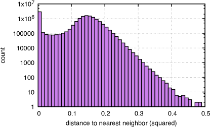
Figure 4: Histogram of distances of the images of Imnet22k to their nearest neighbor.

Images that are bit-wise exact are unambiguous duplicates – in fact they are often already removed beforehand from the datasets because they are easy to detect by computing a hash value on the content. Beyond this extreme case, the notion of “duplicate” is ambiguous: images that are re-encoded, resized, slightly cropped should be considered duplicates, but the case of larger transformations is less obvious (e.g., photos of the same painting, consecutive frames of a video).

TinyNet 1

TinyNet 2

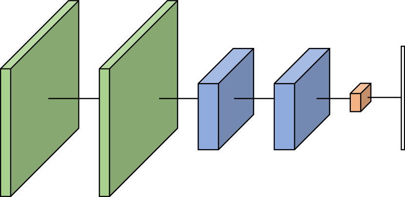
TinyNet 3

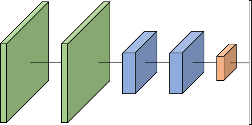
Figure 5: Tiny nets.

B.2 Identification of connected components

We set a conservative arbitrary threshold of $0.001$ to detect duplicate images, and remove the edges of the k-nn graph that are above this threshold. We compute the connected components, and keep a single image per connected component.

For Imnet22k, the largest connected components are error images returned by image banks like Flickr for missing entries. This is an artifact of how the dataset was downloaded. The largest non-trivial cluster from Imnet22k is the image of a flower in Figure 6, that appears in 72 different synsets. There seems to be some disagreement on the species of this flower, along with plain bad annotations.

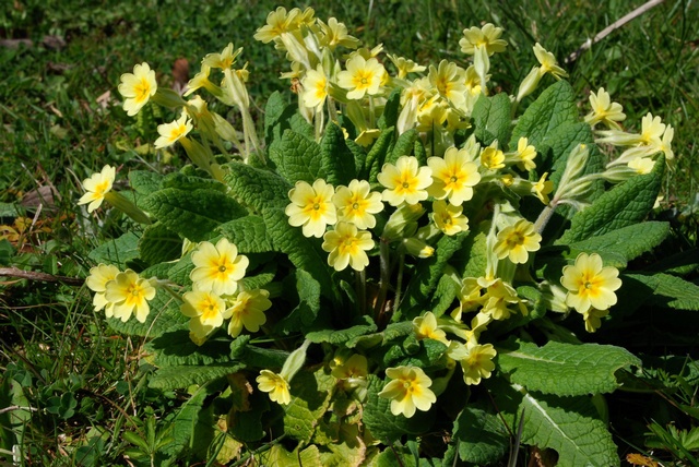
n11610437 bishop pine, bishop’s pine, Pinus muricata n11619455 western larch, western tamarack, Oregon larch, Larix occidentalis n11621281 amabilis fir, white fir, Pacific silver fir, red silver fir, Christmas tree, Abies amabilis n11626826 red spruce, eastern spruce, yellow spruce, Picea rubens n11710827 cucumber tree, Magnolia acuminata n11721642 lesser spearwort, Ranunculus flammula n11722342 western buttercup, Ranunculus occidentalis n11722621 cursed crowfoot, celery-leaved buttercup, Ranunculus sceleratus n11753562 buffalo clover, Trifolium reflexum, Trifolium stoloniferum n11840476 desert four o’clock, Colorado four o’clock, maravilla, Mirabilis multiflora n11874081 yellow rocket, rockcress, rocket cress, Barbarea vulgaris, Sisymbrium barbarea n11882426 crinkleroot, crinkle-root, crinkle root, pepper root, toothwort, Cardamine diphylla, Dentaria diphylla n11887750 western wall flower, Erysimum asperum, Cheiranthus asperus, Erysimum arkansanum n11889205 tansy-leaved rocket, Hugueninia tanacetifolia, Sisymbrium tanacetifolia … …

Figure 6: Image that appears in the largest number of duplicate versions in Imnet22k (72), with a few of the corresponding synsets.

B.3 Statistics

Table 4 shows some statistics on the duplicates identified by our simple approach. Imnet22k has 10.4 % duplicate images. In addition to these duplicates, we removed 930,757 images that overlap with Imnet1k, which means that Imnet1k is not a subset of Imnet22k in this paper. Within Imnet1k, we found 1 % duplicates, which seems small enough not to remove them. For Tiny, we found 9.5 % duplicates and removed them, leaving the dataset with $71,726,550$ unique images.

Table 4: Duplicate statistics for the datasets we use.

Dataset	# images	# groups
Imnet22k	14,197,087	12,720,164
Imnet1k-train	1,281,167	1,267,936
Tiny	79,302,017	71,726,550

Appendix C TinyNet architectures

This appendix describes the convolutional architecture employed in Section 3.2 of the main paper to evaluate the capacity saturation and the influence of training parameters and choices on this capacity.

The architectures includes from 3 convolutional layers for TinyNet1 to 4 for TinyNet2 and TinyNet3. The first convolutional layer is 5x5. Each convolutional layer is followed by a Rectifier Linear Unit activation. The fully connected layer of TinyNet3 is larger than TinyNet2.

Appendix D Filters

$n$=100k, no augmentation

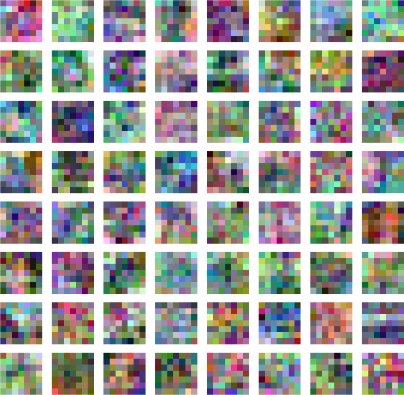
$n$=100k, flip

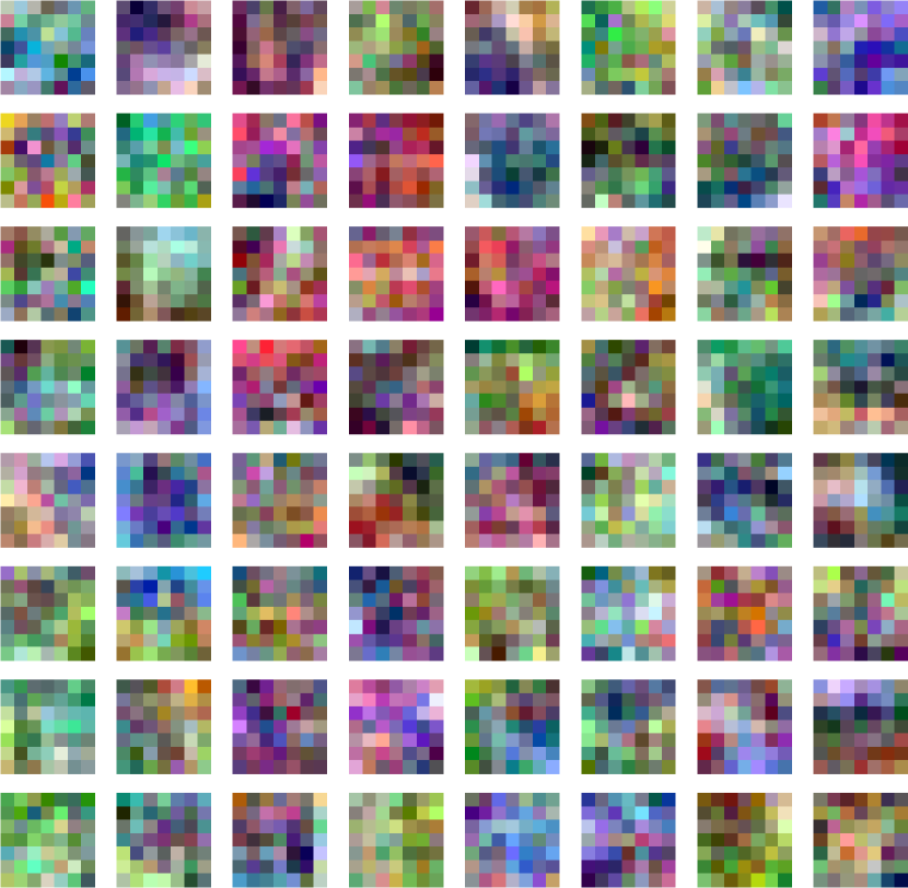
$n$=100k, flip+crop$\pm$2

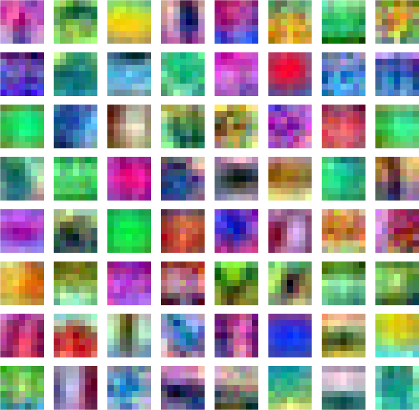
Figure 7: Filters of the first convolutional layer (7x7, 64 filters) obtained when learning to explicitly memorize if an image was used for training or not.

The filters of the first convolutional layer are easy to visualize and contain interesting information on how the SGD optimized to the very first filter that is applied on the image pixels (Krizhevsky et al., 2012; Bojanowski & Joulin, 2017; Paulin et al., 2017). Figure 7 shows the filters obtained after training a Resnet-18. The filters for 10k images are very noisy compared to the smooth Gabor filters produced by supervised classifiers. This is probably due to the large capacity of the network, that is able to quickly overfit the data and does not need to update the filter weights beyond their random initialization. With more images, the filters become more uniform, exhibiting some specialization. Interestingly, for $n$=100k with crop augmentation the filters have a clear uniform color. This is required for the output to be less sensitive to translations of up to 2 pixels.

Appendix E Shadow models

We evaluated the performance of shadow models on the partial-layers setting. The setting is the following: we train $20$ networks on the public dataset, each time holding out a different subset of images. For each network, we can thus compare the activations of train and held-out images. These activations are not directly comparable between two different networks, because internal activations of a ReLU network have invariances (such as permutation of the neurons or positive rescaling). To circumvent this issue, we learn a regression model that maps activations between two networks, and thus align activations of all the networks to the activations of the network under attack using the $\ell_{2}$ loss. We then learn an attack model that predicts from the aligned activations whether the image was seen by the network at train time.

The results are shown in Table 5. While performing better than random guessing, shadow models underperform the attack methods shown in Table 3. We believe that this is due to the complex processing involved in training shadow models on intermediate activations (notably the regression model), whereas the attacks of Section 5 are more straightforward to train.

Table 5: Accuracy of membership inference attacks before the softmax layer of the models (partial-layers), using shadow models.

Model	Augmentation	Attack accuracy
Resnet101	None	60.6
	Flip, Crop $\pm 5$	61.4
	Flip, Crop	58.2
VGG16	None	73.8
	Flip, Crop $\pm 5$	65.8
	Flip, Crop	55.2

References

- Abadi et al. (2016) Martin Abadi, Andy Chu, Ian Goodfellow, H Brendan McMahan, Ilya Mironov, Kunal Talwar, and Li Zhang. Deep learning with differential privacy. In CCS, 2016.
- Abadi et al. (2017) Martín Abadi, Ulfar Erlingsson, Ian Goodfellow, H Brendan McMahan, Ilya Mironov, Nicolas Papernot, Kunal Talwar, and Li Zhang. On the protection of private information in machine learning systems: Two recent approches. In CSF, 2017.
- Ateniese et al. (2015) Giuseppe Ateniese, Luigi V Mancini, Angelo Spognardi, Antonio Villani, Domenico Vitali, and Giovanni Felici. Hacking smart machines with smarter ones: How to extract meaningful data from machine learning classifiers. IJSN, 2015.
- Balu et al. (2014) Raghavendran Balu, Teddy Furon, and Sébastien Gambs. Challenging differential privacy: the case of non-interactive mechanisms. In ESORICS, 2014.
- Bassily et al. (2016) Raef Bassily, Kobbi Nissim, Adam Smith, Thomas Steinke, Uri Stemmer, and Jonathan Ullman. Algorithmic stability for adaptive data analysis. In STOC, 2016.
- Behpour et al. (2017) S. Behpour, K. Kitani, and B. Ziebart. ADA: A game-theoretic perspective on data augmentation for object detection. In arXiv, 2017.
- Biggio et al. (2014) Battista Biggio, Igino Corona, Blaine Nelson, Benjamin I. P. Rubinstein, Davide Maiorca, Giorgio Fumera, Giorgio Giacinto, and Fabio Roli. Security Evaluation of Support Vector Machines in Adversarial Environments. 2014.
- Bojanowski & Joulin (2017) Piotr Bojanowski and Armand Joulin. Unsupervised learning by predicting noise. In ICML, 2017.
- Carlini et al. (2018) Nicholas Carlini, Chang Liu, Jernej Kos, Úlfar Erlingsson, and Dawn Song. The secret sharer: Measuring unintended neural network memorization & extracting secrets. arXiv preprint arXiv:1802.08232, 2018.
- Deng et al. (2009) Jia Deng, Wei Dong, Richard Socher, Li-Jia Li, Kai Li, and Li Fei-Fei. Imagenet: A large-scale hierarchical image database. In Computer Vision and Pattern Recognition, 2009. CVPR 2009. IEEE Conference on, pp. 248–255, 2009.
- Dhamija et al. (2000) Rachna Dhamija, Adrian Perrig, et al. Déjà vu-a user study: Using images for authentication. In USENIX Security Symposium, 2000.
- Dosovitskiy et al. (2014) Alexey Dosovitskiy, Jost Tobias Springenberg, Martin Riedmiller, and Thomas Brox. Discriminative unsupervised feature learning with convolutional neural networks. In NIPS, 2014.
- Douze et al. (2009) Matthijs Douze, Hervé Jégou, Harsimrat Sandhawalia, Laurent Amsaleg, and Cordelia Schmid. Evaluation of gist descriptors for web-scale image search. In CIVR, 2009.
- Dwibedi et al. (2017) Debidatta Dwibedi, Ishan Misra, and Martial Hebert. Cut, paste and learn: Surprisingly easy synthesis for instance detection. In ICCV, 2017.
- Dwork et al. (2006) Cynthia Dwork, Frank McSherry, Kobbi Nissim, and Adam Smith. Calibrating noise to sensitivity in private data analysis. In TCC, 2006.
- Feller (1949) W. Feller. On the kolmogorov-smirnov limit theorems for empirical distributions. Annals of Mathematical Statistics, 1949.
- Hariharan & Girshick (2017) Bharath Hariharan and Ross Girshick. Low-shot visual recognition by shrinking and hallucinating features. In CVPR, 2017.
- Hayes et al. (2017) Jamie Hayes, Luca Melis, George Danezis, and Emiliano De Cristofaro. Logan: evaluating privacy leakage of generative models using generative adversarial networks. arXiv preprint arXiv:1705.07663, 2017.
- He et al. (2016) Kaiming He, Xiangyu Zhang, Shaoqing Ren, and Jian Sun. Deep residual learning for image recognition. In CVPR, 2016.
- He et al. (2017) Kaiming He, Georgia Gkioxari, Piotr Dollár, and Ross Girshick. Mask R-CNN. In ICCV, 2017.
- Hinton et al. (1986) Geoffrey E Hinton, James L McClelland, David E Rumelhart, et al. Distributed representations. Parallel distributed processing: Explorations in the microstructure of cognition, 1986.
- Hopfield (1982) John J Hopfield. Neural networks and physical systems with emergent collective computational abilities. PNAS, 1982.
- Iscen et al. (2017) Ahmet Iscen, Teddy Furon, Vincent Gripon, Michael Rabbat, and Hervé Jégou. Memory vectors for similarity search in high-dimensional spaces. IEEE Trans. Big Data, 2017.
- Johnson et al. (2017) Jeff Johnson, Matthijs Douze, and Hervé Jégou. Billion-scale similarity search with gpus. arXiv preprint arXiv:1702.08734, 2017.
- Kraska et al. (2017) Tim Kraska, Alex Beutel, Ed H Chi, Jeffrey Dean, and Neoklis Polyzotis. The case for learned index structures. arXiv preprint arXiv:1712.01208, 2017.
- Krizhevsky et al. (2012) Alex Krizhevsky, Ilya Sutskever, and Geoffrey E Hinton. Imagenet classification with deep convolutional neural networks. In Advances in neural information processing systems, pp. 1097–1105, 2012.
- Krogh & Hertz (1991) A. Krogh and J. A. Hertz. A simple weight decay can improve generalization. In NIPS, 1991.
- Krueger et al. (2017) David Krueger, Nicolas Ballas, Stanislaw Jastrzebski, Devansh Arpit, Maxinder S. Kanwal, Tegan Maharaj, Emmanuel Bengio, Asja Fischer, Aaron Courville, Simon Lacoste-Julien, and Yoshua Bengio. A closer look at memorization in deep networks. In ICML, 2017.
- LeCun et al. (1990) Yann LeCun, Bernhard E Boser, John S Denker, Donnie Henderson, Richard E Howard, Wayne E Hubbard, and Lawrence D Jackel. Handwritten digit recognition with a back-propagation network. In NIPS, 1990.
- Lenc & Vedaldi (2015) Karel Lenc and Andrea Vedaldi. Understanding image representations by measuring their equivariance and equivalence. In CVPR, 2015.
- Long et al. (2018) Yunhui Long, Vincent Bindschaedler, Lei Wang, Diyue Bu, Xiaofeng Wang, Haixu Tang, Carl A Gunter, and Kai Chen. Understanding membership inferences on well-generalized learning models. arXiv preprint arXiv:1802.04889, 2018.
- MacKay (2002) David J. C. MacKay. Information Theory, Inference & Learning Algorithms. 2002.
- Mahendran & Vedaldi (2015) Aravindh Mahendran and Andrea Vedaldi. Understanding deep image representations by inverting them. In CVPR, 2015.
- Oliva & Torralba (2006) Aude Oliva and Antonio Torralba. Building the gist of a scene: The role of global image features in recognition. Progress in brain research, 2006.
- Paulin et al. (2014) Mattis Paulin, Jérôme Revaud, Zaid Harchaoui, Florent Perronnin, and Cordelia Schmid. Transformation pursuit for image classification. In CVPR, 2014.
- Paulin et al. (2017) Mattis Paulin, Julien Mairal, Matthijs Douze, Zaid Harchaoui, Florent Perronnin, and Cordelia Schmid. Convolutional patch representations for image retrieval: an unsupervised approach. IJCV, 2017.
- Personnaz et al. (1986) L Personnaz, I Guyon, and G Dreyfus. Collective computational properties of neural networks: New learning mechanisms. Physical Review A, 1986.
- Plate (1995) Tony A Plate. Holographic reduced representations. IEEE Transactions on Neural networks, 1995.
- Rubinstein et al. (2009) Benjamin IP Rubinstein, Peter L Bartlett, Ling Huang, and Nina Taft. Learning in a large function space: Privacy-preserving mechanisms for SVM learning. arXiv:0911.5708, 2009.
- Russakovsky et al. (2015) Olga Russakovsky, Jia Deng, Hao Su, Jonathan Krause, Sanjeev Satheesh, Sean Ma, Zhiheng Huang, Andrej Karpathy, Aditya Khosla, Michael Bernstein, Alexander C. Berg, and Li Fei-Fei. ImageNet Large Scale Visual Recognition Challenge. IJCV, 2015.
- Shokri et al. (2016) Reza Shokri, Marco Stronati, and Vitaly Shmatikov. Membership inference attacks against machine learning models. CoRR, abs/1610.05820, 2016.
- Simonyan & Zisserman (2014) Karen Simonyan and Andrew Zisserman. Very deep convolutional networks for large-scale image recognition. In ICLR, 2014.
- Srivastava et al. (2014) Nitish Srivastava, Geoffrey Hinton, Alex Krizhevsky, Ilya Sutskever, and Ruslan Salakhutdinov. Dropout: A simple way to prevent neural networks from overfitting. 2014.
- Thomee et al. (2016) Bart Thomee, David A. Shamma, Gerald Friedland, Benjamin Elizalde, Karl Ni, Douglas Poland, Damian Borth, and Li-Jia Li. YFCC100M: The new data in multimedia research. Communications of the ACM, 2016.
- Tommasi et al. (2017) Tatiana Tommasi, Novi Patricia, Barbara Caputo, and Tinne Tuytelaars. A deeper look at dataset bias. In Domain Adaptation in Computer Vision Applications. 2017.
- Torralba & Efros (2011) Antonio Torralba and Alexei A Efros. Unbiased look at dataset bias. In CVPR, 2011.
- Torralba et al. (2008) Antonio Torralba, Rob Fergus, and William T Freeman. 80 million tiny images: A large data set for nonparametric object and scene recognition. IEEE Trans. PAMI, 2008.
- Ulyanov et al. (2017) Dmitry Ulyanov, Andrea Vedaldi, and Victor Lempitsky. Deep image prior. arXiv:1711.10925, 2017.
- Wang et al. (2016) Yu-Xiang Wang, Jing Lei, and Stephen E Fienberg. On-average KL-privacy and its equivalence to generalization for max-entropy mechanisms. In International Conference on Privacy in Statistical Databases. Springer, 2016.
- Yeom et al. (2018) Samuel Yeom, Irene Giacomelli, Matt Fredrikson, and Somesh Jha. Privacy risk in machine learning: Analyzing the connection to overfitting. arXiv preprint arXiv:1709.1604, 2018.
- Zeiler & Fergus (2014) Matthew D Zeiler and Rob Fergus. Visualizing and understanding convolutional networks. In ECCV. Springer, 2014.
- Zhang et al. (2016) Chiyuan Zhang, Samy Bengio, Moritz Hardt, Benjamin Recht, and Oriol Vinyals. Understanding deep learning requires rethinking generalization. arXiv preprint arXiv:1611.03530, 2016.