The delay of shock breakout due to circumstellar material seen in most Type II Supernovae

Authors:

F. Förster^1,2,3∗, T. J. Moriya⁴, J.C. Maureira¹, J.P. Anderson⁵, S. Blinnikov^6,7,8, F. Bufano⁹, G. Cabrera–Vives^10,2, A. Clocchiatti^11,2, Th. de Jaeger¹², P.A. Estévez^2,13, L. Galbany¹⁴, S. González–Gaitán^1,15, G. Gräfener¹⁶, M. Hamuy^2,3, E. Hsiao¹⁷, P. Huentelemu¹³, P. Huijse^2,18, H. Kuncarayakti^19,20, J. Martínez-Palomera^3,2,1, G. Medina³, F. Olivares E.^2,3, G. Pignata^21,2, A. Razza^3,5, I. Reyes^13,2, J. San Martín¹, R.C. Smith²², E. Vera¹, A.K. Vivas²², A. de Ugarte Postigo^23,24, S.-C. Yoon^25,26, C. Ashall²⁷, M. Fraser²⁸, A. Gal–Yam²⁹, E. Kankare³⁰, L. Le Guillou³¹, P.A. Mazzali^27,32, N.A. Walton³³, D.R. Young^30
1Center for Mathematical Modeling, University of Chile; ²Millennium Institute of Astrophysics, Chile; ³Department of Astronomy, University of Chile; ⁴Division of Theoretical Astronomy, National Astronomical Observatory of Japan, National Institutes of Natural Sciences, 2-21-1 Osawa, Mitaka, Tokyo 181-8588, Japan ⁵European Southern Observatory, Alonso de Córdova 3107, Casilla 19, Santiago, Chile; ⁶Kavli Institute for the Physics and Mathematics of the Universe (WPI), University of Tokyo, Japan; ⁷Institute for Theoretical and Experimental Physics (ITEP), Moscow, Russia; ⁸All-Russia Research Institute of Automatics (VNIIA), Moscow, Russia ⁹INAF - Astrophysical Observatory of Catania, Italy; ¹⁰Department of Computer Science, University of Concepción, Chile; ¹¹Department of Physics and Astronomy, Universidad Católica de Chile, Santiago, Chile ¹²Department of Astronomy, University of California Berkeley, USA; ¹³Department of Electrical Engineering, University of Chile; ¹⁴Department of Physics and Astronomy, University of Pittsburgh, USA; ¹⁵CENTRA, Instituto Técnico Superior, Universidade de Lisboa, Portugal; ¹⁶Argelander-Institut fur Astronomie, Auf dem Hügel 71, D-53121 Bonn, Germany; ¹⁷Department of Physics, Florida State University, USA; ¹⁸Informatics Institute, Universidad Austral de Chile; ¹⁹Finnish Centre for Astronomy with ESO (FINCA), University of Turku, Väisäläntie 20, 21500 Piikkiö, Finland; ²⁰Tuorla Observatory, Department of Physics and Astronomy, University of Turku, Väisäläntie 20, 21500 Piikkiö, Finland ²¹Departamento de Ciencias Fisicas, Universidad Andres Bello, Avda. República 252, Santiago, Chile ²²Cerro Tololo Interamerican Observatory, La Serena, Chile; ²³Instituto de Astrofísica de Andalucía (IAA-CSIC), Glorieta de la Astronomía, s/n 18008 Granada, Spain ²⁴Dark Cosmology Centre, Niels Borh Institute, University of Copenhagen, Juliane Maries Vej 30, 2100 Copenhagen Ø, Denmark ²⁵Department of Physics and Astronomy, Seoul National University, Gwanak-ro1, Gwanakgu, Seoul 08826, South Korea ²⁶Monash Centre for Astrophysics, School of Physics and Astronomy, Monash University, VIC 3800, Australia ²⁷Astrophysics Research Institute, Liverpool John Moores University, IC2, Liverpool Science Park, 146 Brownlow Hill, Liverpool L3 5RF, UK ²⁸School of Physics, O’Brien Centre for Science North, University College Dublin, Belfield, Dublin 4, Ireland. ²⁹Department of Particle Physics and Astrophysics, Weizmann Institute of Science, Rehovot 76100, Israel. ³⁰Astrophysics Research Centre, School of Mathematics and Physics, Queens University Belfast, Belfast BT7 1NN, UK ³¹Sorbonne Université, Univ Paris 06 (UPMC), Université Paris Diderot, CNRS, IN2P3, UMR 7585, LPNHE, Laboratoire de Physique Nucléaire et de Hautes Energies, Paris, France ³²Max-Planck-Institut fur Astrophysik, Karl-Schwarzschild-Str. 1, 85748 Garching bei Munchen, Germany ³³Institute of Astronomy, University of Cambridge, Madingley Road, Cambridge CB3 0HA, UK

Type II supernovae (SNe) originate from the explosion of hydrogen–rich supergiant massive stars. Their first electromagnetic signature is the shock breakout, a short–lived phenomenon which can last from hours to days depending on the density at shock emergence. We present 26 rising optical light curves of SN II candidates discovered shortly after explosion by the High cadence Transient Survey (HiTS) and derive physical parameters based on hydrodynamical models using a Bayesian approach. We observe a steep rise of a few days in 24 out of 26 SN II candidates, indicating the systematic detection of shock breakouts in a dense circumstellar matter consistent with a mass loss rate $\dot{M}>10^{-4}$ $M_{\odot}$ yr^-1 or a dense atmosphere. This implies that the characteristic hour timescale signature of stellar envelope SBOs may be rare in nature and could be delayed into longer–lived circumstellar material shock breakouts in most Type II SNe.

With a new generation of large etendue facilities such as iPTF [1], SkyMapper [2], Pan–STARRS [3], KMTNET [4], ATLAS [5], DECam [6], Hyper Suprime–Cam [7], ZTF [8] or LSST [9] the study of rare and short–lived phenomena in large volumes of the Universe is becoming possible. This allows not only finding new classes of events, but also systematically studying short–lived phases of evolution in known astrophysical phenomena, such as SN explosions. In this work we present 26 rising optical light curves from Type IIP/L SN candidates discovered shortly after explosion by the High cadence Transient Survey (HiTS) [10, hereafter F16], and a systematic study of their physical properties.

Type IIP/L SNe, hereafter SNe II, are thought to originate after the core collapse of massive red supergiant stars (RSGs) with main sequence masses between 8 $M_{\odot}$ and 16.5 $M_{\odot}$ [11], although see [12]. In the currently favored scenario, the neutrino–driven mechanism (see [13] and references therein), a small fraction of the gravitational energy lost during collapse is transferred to the outer layers of the star via neutrino heating. This triggers a shock wave which, depending on the mass of the progenitor and the total input energy, can sometimes unbind the envelope of the star in a SN explosion. This shock wave is radiation dominated, Compton scattering mediated and propagates supersonically, typically at tens of thousands of km/s [14]. The shock precursor has a characteristic optical depth, estimated equating the timescales for photons to diffuse out of the shock front (diffusion timescale) and the timescale for the shock to move into a new region of the star (advection timescale), of $\tau\approx c/v_{\rm shock}$, where $c$ is the speed of light and $v_{\rm shock}$ is the shock propagation speed [15]. This can be written as a distance of about 30 times the mean free path of a photon scattering off electrons and it is therefore proportional to the electron density.

In RSGs, the shock is expected to travel for about a day until it reaches an optical depth from infinity small enough for the shock to emerge. For example, a shock traveling at 10,000 km/s would take 19 hours to traverse 1,000 $R_{\odot}$. The emergence of the shock itself, or shock breakout (SBO, see review in [16]), should typically last for about an hour if it happens from the envelope of a RSG, a timescale which is determined by the width of the shock precursor (proportional to density), the shock velocity and some form factors. We call this scenario an envelope SBO, e.g. [17].

If a dense wind or atmosphere is present, the ejecta’s photosphere at shock emergence can extend beyond the typical RSG sizes predicted by stellar evolution theory. This can push shock emergence radially outwards into lower electron densities, where the shock’s radiative precursor will be significantly more extended for the same optical depth and will therefore have a longer–lived emergence. Thus, apart from powering the early light curve via conversion of kinetic energy into radiation, this dense circumstellar material (CSM) can delay the shock emergence and extend its duration to several days due to both the lower electron density and light travel time effects, replacing the much shorter–lived envelope SBO. We call this scenario a wind SBO [18, 19, 20, 21, 22] or extended atmosphere SBO [23].

After shock emergence, the envelope of RSGs should adiabatically cool until recombination of hydrogen starts. As the RSG envelope expands and cools, its typical temperature enters the optical range in a timescale of several days, making SNe II optical light curves (LCs) rise up to maximum light with a timescale of about 7 days [24], with possible sub–classes of relatively slow and fast rising SNe II [25]. This timescale has been used to derive typical RSG stellar radii using analytic approximations or hydrodynamical models. The observed rise timescales are shorter than expected and have led researchers to conclude that either the radii of RSGs are much smaller than predicted by stellar evolution theory [24, 26], or that perhaps a dense wind SBO is responsible for the fast rise. The latter is supported by the early spectroscopic detection of narrow optical emission lines with broad electron–scattering wings in SN2013fs [22], which are suggestive of slowly moving shocked material [23]; and by a recent analysis of type II SN light curves around maximum light [27]. Thus, it is important to understand the innermost regions of the wind or extended atmospheres of RSGs.

There have been several observational efforts to discover RSG envelope SBOs using high cadence observations from space [28, 29, 30, 31] and ground–based observatories [32] from the UV to optical wavelengths, but only marginal detections have been achieved (a notable exception was the serendipitous discovery of the envelope stripped SN IIb 2016gkg [33]). HiTS (F16) is a survey which uses the Dark Energy Camera (DECam) to explore the transient sky in timescales from hours to weeks, monitoring the hour timescale transient sky during three observational campaigns in 2013, 2014 and 2015.

Observations and data processing

The observational strategy of HiTS is described in F16. In 2013 we surveyed 120 deg² in the $u$–band with a cadence of 2 hours during 4 consecutive nights. In 2014 and 2015 we surveyed 120 and 150 deg², with a cadence of 2 and 1.6 hours during 5 and 6 consecutive nights, respectively. In 2015 the high cadence phase was followed by a few observations days later, mostly in $g$, but also in $r$ band. The 2014 and 2015 data were analyzed in real–time, with candidates being generated and filtered only minutes after the end of every exposure. Thanks to these real–time capabilities, in 2014 and 2015 we were able to trigger spectroscopic follow–up observations for a few of the most nearby candidates, with hour timescale spectroscopic follow up capabilities in 2015 using the Very Large Telescope. No clear signatures of envelope SBOs were found and the very fast spectroscopic observations were never triggered, but we obtained spectra for 18 objects after the main high cadence phase of the observations for classification purposes: using NTT (provided by the PESSTO collaboration [34]), SOAR and VLT (see Methods). These spectra were used for direct classification, but also for testing a LC based classifier. 11 SN candidates were spectroscopically classified as SNe Ia and 7 SN candidates were classified as either SNe II or showed a blue continuum consistent with SNe II.

The DECam data processing from raw image to light curve creation is discussed in Methods. Although the resulting LCs did not show the signature of envelope SBOs it was evident that the first few days of evolution of synthetic light curves which do not include CSM, and which show an hour timescale SBO signature, did not resemble our observations. In order to investigate this further we used models from [20, 21] (hereafter M18), which include CSM, and developed tools that can be used to aid the classification and physical interpretation of these LCs.

Light curve based classification

When no spectral information could be acquired we used the SN early LCs for classification. Since our LCs are based on image differences, which sometimes contain a very recent template, our observables are LC differences between two points in time, i.e. we take into account that our templates can contain some SN flux. Comparing these observables against model predictions for a class of events we can perform model selection and classification. For the RSG SNe II we use the family of models from M18. The most important remaining classes are thermonuclear SNe (Ia) and envelope–stripped core collapse SNe (Ib/c), which in most cases are explosions whose rise to maximum is dominated by the deposition of energy from ⁵⁶Ni starting from a compact configuration [35]. Therefore, as a simple approximation we use SN Ia spectral templates from [36] and allow for a broad range of stretch and scale factors to account for greater diversity. Then, using a Markov Chain Monte Carlo (MCMC) sampler (as explained in Methods) we compute a median log–likelihood for these two families of models and select between them using the Bayesian Information Criterion (BIC). With this method we correctly classify all 18 SNe with spectroscopic classification: 7 SNe II and 11 SNe Ia (see Figure 1), which highlights the power of using early time photometry for classification.

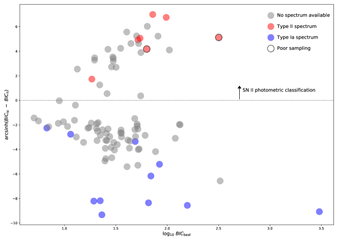
Figure 1: Light curve based classification implemented in this work. We show the arcsinh of the BIC differences between our SN II and SN I models as discussed in the text. Note that all SNe with spectroscopic information were correctly classified. There were two SNe with spectra which were not included in the analysis because of their poor sampling at rise.

We removed SNe which had a maximum time span of less than one week, which eliminated all candidates from 2013A and one SN with spectra from 2014A. Also, since we are mostly interested in the effect of mass loss and wind acceleration, which affect mostly the initial rise after emergence, we remove those SNe with a poor sampling at rise. We define a poor sampling at rise as those cases where three or more continuous days during rise have no data. This includes SNe which have gaps in the data of two or more consecutive nights during the initial rise (5 SNe discovered at the end of the 15A campaign, which had a logarithmic cadence); and SNe where we cannot rule out that they were seen only three or more days after their first light. For the latter case we remove those SNe that according to our posterior distribution had more than 10% probability of having been observed only three or more days after first light, defining the first light as the moment when the absolute magnitude in $g$ band reaches -13 mag. This additional filter resulted in the removal of two SNe.

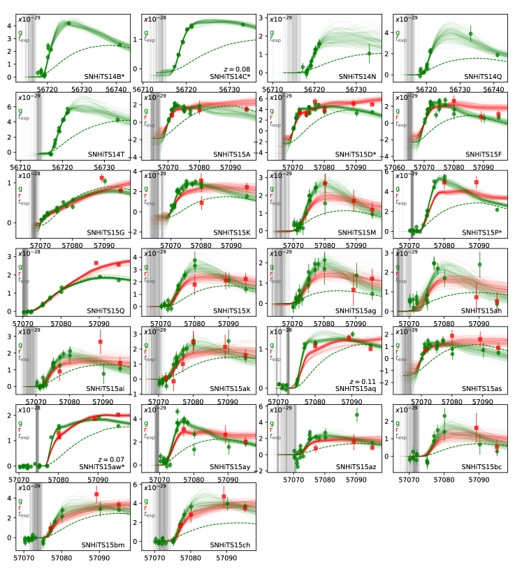
Figure 2: Observation minus template flux in [erg/s/cm²/Hz] vs MJD time for the Type II SN candidates in $g$ (green circles) and $r$ (red squares) bands with 1–$\sigma$ error bars. Flux differences from 100 models randomly sampled from the posterior are shown (continuous lines with the same colors per band), including one $g$ band example with mass loss rate set to zero (green dashed lines). Explosion times are indicated by the vertical gray lines. SNe with spectroscopic classification are shown with an asterisk, and spectroscopic host galaxy redshifts are indicated when available. Most SNe show a steep initial rise, the signature of the wind shock breakout.

Early SN II light curves and models

The resulting sample of 26 early time SN II candidate LCs discovered by the HiTS survey are shown in Figure 2. There is no similar sample of SN II early LCs in the literature in terms of cadence, i.e. every 2 or 1.6 hours during the night for several consecutive nights, and size. We will include five additional SNe II from the literature in the analysis, all with well sampled optical early light curves: SN2006bp [37], PS1-13arp [19], SN2013fs [22], KSN2011a and KSN2011d [30]. The SN II candidates show a fast rise with a timescale of a few days which is suggestive of the wind / extended atmosphere SBO scenario [19, 20, 23]. We also show for comparison 100 LCs sampled from the posterior distribution of physical parameters using a grid of SN II explosion models from M18. Briefly, we sample the posterior distribution of physical parameters such as explosion time, attenuation, redshift, progenitor mass, explosion energy, mass loss rate ($\dot{M}$) and wind acceleration parameter ($\beta$), using a MCMC sampler as explained in the Suppplementary Information. For reference, we also show one $g$ band LC sampled randomly from the posterior where we have set the mass loss to zero. It can be seen that for most LCs only models with a significant mass loss rate match the fast rise observed in the data.

Synthetic models

Models from M18 assume confined steady–state winds with an extended acceleration length scale. They form a grid of 518 sets of spectral time series spanning different main sequence masses and explosion energies, but also different mass loss properties. The RSG SN progenitors and the CSM around them are constructed in the same way as in M18. We provide a short summary of the progenitors and CSM.

The public stellar evolution code MESA [38, 39, 40] is used to compute the RSG SN progenitors of the zero-age main-sequence (ZAMS) masses of 12, 14, and $16~{}M_{\odot}$ with solar metallicity. We set the model maximum mass to $16~{}M_{\odot}$ because the maximum mass of SN II progenitors is estimated to be at around $16.5~{}M_{\odot}$ based on the RSG progenitor detections [11]. The progenitors are evolved by using the Ledoux criterion for convection with a mixing-length parameter of 2.0 and a semiconvection parameter of 0.01. Overshooting is taken into account on top of the hydrogen-burning convective core with a step function using the overshoot parameter of $0.3H_{P}$, where $H_{P}$ is the pressure scale height. We use the ‘Dutch’ mass-loss prescription in MESA without scaling for both hot and cool stars. The RSG progentiors are evolved to the core oxygen burning, from which the hydrogen-rich envelope structure hardly changes until the core collapse. The final progenitor properties are summarized in Table 1.

ZAMS mass	Final mass	Final H-rich envelope mass	Final radius
$12~{}M_{\odot}$	$10.3~{}M_{\odot}$	$6.1~{}M_{\odot}$	$607~{}R_{\odot}$
$14~{}M_{\odot}$	$11.4~{}M_{\odot}$	$6.2~{}M_{\odot}$	$832~{}R_{\odot}$
$16~{}M_{\odot}$	$12.0~{}M_{\odot}$	$5.8~{}M_{\odot}$	$962~{}R_{\odot}$

Table 1: RSG progenitor properties.

A CSM structure with density $\rho_{\mathrm{CSM}}(r)=\dot{M}/(4\pi v_{\mathrm{wind}})r^{-2}$ is attached on top of these progenitors. Here, $\dot{M}$ is the progenitor’s mass-loss rate, $r$ is the distance from the center of the star and $v_{\mathrm{wind}}$ is the wind velocity. We do not change $\dot{M}$ with $r$ in our models. Instead of $\dot{M}$, we take the radial change of $v_{\mathrm{wind}}$ caused by the wind acceleration into account. The simple $\beta$ velocity law for the wind velocity, i.e.,

$$v_{\mathrm{wind}}(r)=v_{0}+(v_{\infty}-v_{0})\left(1-\frac{R_{0}}{r}\right)^{\beta},$$ (1)

where $v_{0}$ is the initial wind velocity, $v_{\infty}$ is the terminal wind velocity, and $R_{0}$ is the wind launching radius that we set at the stellar surface, is adopted. $v_{\infty}=10~{}\mathrm{km~{}s^{-1}}$ is fixed in our models. $v_{0}$ is chosen so that the CSM density is smoothly connected from the surface of the progenitors and it is less than $10^{-2}~{}\mathrm{km~{}s^{-1}}$. We take $\beta$ between 1 and 5 because OB stars have $\beta\simeq 0.5-1$ [41] and RSGs are known to experience slower wind acceleration than OB stars, i.e., $\beta>1$ e.g. [42, 43]. For instance, a RSG $\zeta$ Aurigae is known to have $\beta\simeq 3.5$ [44].

          

          

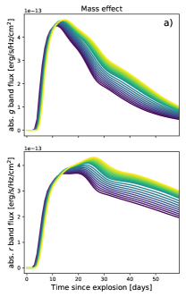
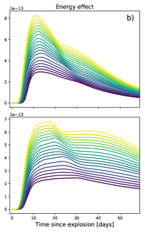
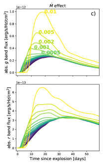
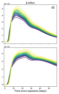
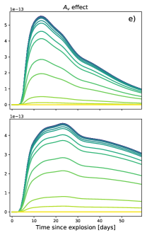
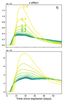
Figure 3: Interpolated synthetic absolute fluxes (obtained from the predicted apparent magnitude minus the distance modulus) in the $g$ and $r$ bands after varying the progenitor mass linearly between 12 and 16 $M_{\odot}$ (a), the energy linearly between 0.5 and 2 B (b), $\dot{M}$ logarithmically between $10^{-8}$ and $10^{-2}$ $M_{\odot}$ yr^-1 (c), $\beta$ linearly between 1 and 5 (d), $A_{V}$ logarithmically between $10^{-4}$ and $10$, and $z$ logarithmically between 0.001 and 1. $\dot{M}=0$ is arbitrarily associated to $10^{-8}$ $M_{\odot}$ yr^-1 in order to perform the logarithmic interpolation. Values range from blue to yellow in an increasing array of 19 values for each parameter being varied (selected values shown for $\dot{M}$ and $z$). The parameters not being varied are fixed at a mass of 14 $M_{\odot}$, energy of 1 B, $\dot{M}$ of $5\times 10^{-3}$ $M_{\odot}$ yr^-1, $\beta$ of 3.5, $A_{V}$ of 0.1, and redshift of 0.22.

RSG mass loss rates are known to be dependent on the luminosity of the progenitor star, but estimations differ greatly in the literature. For the typical luminosities observed in RSG SN II progenitors, between $10^{4}$ an $10^{5}$ $L_{\odot}$ [11], derived mass mass loss rates range from between $10^{-7}$ and $10^{-6}$  $M_{\odot}$ yr^-1 [45] to between $10^{-5}$ and $10^{-4}$  $M_{\odot}$ yr^-1 [46]. The M18 models assume a wider range of mass loss rates, including zero mass loss and a range of values between $10^{-5}$ and $10^{-2}$ $M_{\odot}$ yr^-1, always assuming enhanced mass loss episodes before explosion extending up to $10^{15}$ cm from the progenitor. Note that a shock travelling at 10,000 km/s would take about 11 days to cover $10^{15}$ cm. Recent optical and X-ray modeling of the SN IIP 2013ej suggests that the dense CSM radius may be relatively small ($10^{14}$ cm), although there are some model uncertainties [47].

Hydrodynamics and radiative transfer

The LCs from the explosions of the above mentioned progenitors with CSM are numerically obtained by using the one-dimensional multi-group radiation hydrodynamics code STELLA [48, 49, 50]. STELLA follows the evolution of the spectral energy distributions (SEDs) at each time step and the multi-color LCs from the explosions are obtained by convolving the filter functions to the numerical SEDs. We use the standard setup for the SED resolution, i.e., 100 bins that are distributed between 1 Å and 50000 Å in a log scale. The code initiates the explosions as thermal bombs. All the models have $0.1~{}M_{\odot}$ of the radioactive ⁵⁶Ni at the center but it does not affect the early LCs we are interested in. Every progenitor model with CSM is exploded with four different explosion energies to investigate the dependence on the explosion energy; $5\times 10^{50}$ erg, $10^{51}$ erg, $1.5\times 10^{51}$ erg, and $2\times 10^{51}$ erg. The effects of mass, energy, mass loss rate, wind acceleration parameter, attenuation and redshift on the optical light curves can be seen in Figure 3.

Results

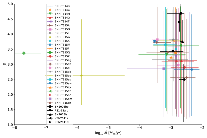
Figure 4: Distribution of inferred $\beta$ and $\dot{M}$ values for the sample of 26 early SNe II candidates from HiTS, as well as selected SNe II from the literature with well sampled optical early light curves (see Figure 5). The error bars correspond to the percentiles 5, 50 and 95 of the marginalized posterior distributions in $\beta$ and $\dot{M}$. Note that the available models range from no mass loss, which we arbitrarily assign 10^-8 $M_{\odot}$ yr^-1, to larger values in a grid between $10^{-5}$ and $10^{-2}$ $M_{\odot}$ yr^-1. Models between $10^{-8}$ and $10^{-5}$ $M_{\odot}$ yr^-1 are logarithmically interpolated between the zero and $10^{-5}$ $M_{\odot}$ yr^-1 mass loss models.

Early time SN II optical LCs are affected by many physical parameters (see Figure 3). These can change the light curve normalization, its characteristic rise time and general shape, the ratio between bands or a combination of them. The parameters which affect the normalization the most are first redshift and $A_{V}$, and then mass loss rate and energy (factor of 10 difference in peak apparent $g$ mag range for the full grid of values tested). The parameters which affect the light curve shape the most are the mass loss rate and redshift, with somewhat similar effects, but very different normalizations which help break their degeneracy. Mass and $\beta$ also affect the normalization, light curve shape and color, but not as strongly as the other variables.

In this work we have concentrated on those variables constraining the CSM density profile, which in the M18 models used in this work is parametrized via two numbers: $\dot{M}$ and $\beta$, assuming a terminal wind velocity of 10 km/s and and a maximum CSM radius of $10^{15}$ cm. Therefore, we focus the discussion on these last two quantities.

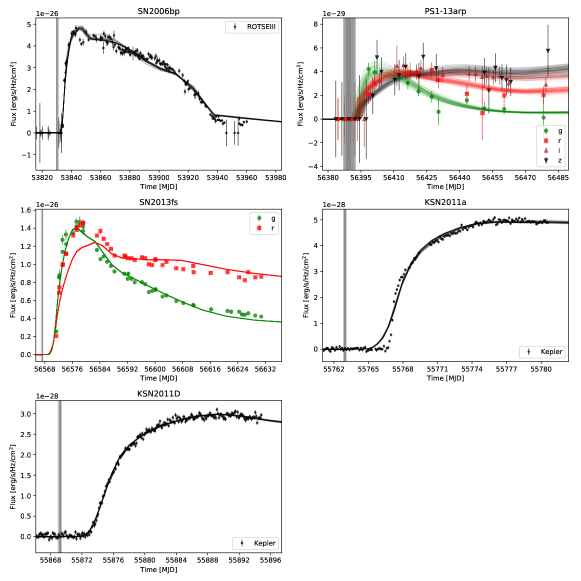
Figure 5: Similar to Figure 3, but for selected SNe II from the literature with well sampled optical early light curves: SN2006bp [37]; PS1-13arp [19]; SN2013fs [22]; KSN2011a and KSN2011d [30] in the indicated bands. The 5, 50 and 95 percentiles for the mass loss and wind acceleration marginalized posterior distributions are shown in Figure 4.

The posterior distributions of $\dot{M}$ and $\beta$ for the entire sample of HiTS SN II candidates, as well as five additional SNe II from the literature with well sampled optical early light curves are summarized in Figure 4. In the $x$ and $y$ axis we show the 5, 50 and 95 percentiles of the marginalized posterior distributions over all variables except $\dot{M}$ or $\beta$, respectively (error bars cover the percentiles 5 to 95, and they intersect at percentiles 50). Mass loss rates smaller than $\dot{M}=10^{-4}$ $M_{\odot}$ yr^-1 are allowed in only two out of 26 HiTS SNe II candidates, and in none of the five SNe II from the literature. We also constrain $\beta$ within the range of values covered by our grid of models ($1<\beta<5$). Although we find significantly large values of $\beta$ for some SNe, we do not find a significant excess of large values within the interval $1<\beta<5$ in the sample. The literature comparison light curves and their posterior sampled synthetic light curves are shown in Figure 5. The complete list of inferred parameters are shown in Supplementary Tables 1 and 2.

We have found evidence for a density profile consistent with large mass loss rates $\dot{M}>10^{-4}$ $M_{\odot}$ yr^-1 in 29 out of 31 SNe II and evidence for a density profile consistent with relatively slow wind acceleration (large $\beta$) for some SNe. These constraints suggest that CSM densities in the vicinity of RSGs before explosion are larger than $10^{-13}$ g cm^-3 at $10^{14}$ cm from the center of the star (about 1400 $R_{\odot}$). Assuming an electron scattering opacity consistent with fully ionized CSM made of hydrogen and helium at solar abundance ($\kappa\ =\ 0.34\ {\rm cm}^{2}~{}{\rm g}^{-1}$), the optical depth $\tau\approx 1$ would occur at typical radii between $10^{14}$ and $10^{15}$ cm and at typical densities between $10^{-12}$ and $10^{-14}$ g cm^-3. The typical densities implied from this analysis are in very good agreement with those derived spectroscopically for SN2013fs in [22], and the mass loss rates are consistent with those derived using NUV data for PS1-13arp.

The large mass loss rates derived in this work imply total CSM masses typically between 0.1 and 1.0 $M_{\odot}$, and typically between 0.01 and 0.1 $M_{\odot}$ above the breakout radius ($\tau\leq c/v$). These mass loss rates could not be sustained for large periods of time before explosion as noted by [22], otherwise we would see Type IIn–like features at late times (narrow optical emission lines with electron scattering wings) and the progenitor star would lose its H–rich envelope before explosion. This favors the interpretation of dense atmospheres or confined accelerated wind SBOs. However, it is interesting to note that the large derived mass loss rates appear to match those from the Type IIb SN2013cu [51, 52, 53], a likely post–RSG star [53]. The fact that most of this CSM would be optically thick at breakout implies that apart from delaying the SBO, most of the shocked material would contribute to the optical light curve via its cooling after breakout. In fact, the differences between LCs with varying CSM radii in [21] are in part explained by this effect.

The range of wind acceleration parameter $\beta$ favored by these observations is consistent with those derived for many normal RSGs [54]. However, models assume enhanced mass loss before explosion and our observations cannot be used to discard whether such enhanced mass loss is required to produce the high density CSM being shocked. The large mass loss rates suggest that either RSGs undergo this enhanced mass loss before explosion or that we are probing complex RSG atmospheres and not an accelerated wind. The fact that high resolution observations of nearby RSGs show complex CSM environments [55] suggests that large CSM densities may in fact be possible without requiring accelerated or enhanced mass loss.

An important implication from this work is that if high CSM densities are present in most SNe II, the hour timescale, high density RSG envelope SBOs may be rare in nature. With the exception of two slow rising SNe out of 26 SN II candidates, large CSM densities were always inferred (see Methods for the significance of this result). The photons produced when the shock crosses the outer envelope of these stars and enters the high density CSM would not be able to diffuse in a timescale of hours, but would instead take days to emerge in the wind SBO. Only if the CSM radii are much smaller than the values tested in this work could a short timescale signature be observed (see Figure 7 in [21]). Given that we have found breakout densities to be similar for different CSM density profiles, measuring the lag between the time of explosion (via neutrinos or gravitational waves in a nearby SNe II) and shock emergence (from one to 12 days after explosion in the parameter space probed by M18), could greatly help understand the true extent of the CSM.

These results also suggest that pre–explosion radii cannot be derived using the early LC of SNe II, at least at the optical bands, because the rise to maximum will not be dominated by the adiabatic cooling of the envelope, but by the wind SBO instead. Furthermore, we have shown that it is possible to accurately separate compact (SNe I) from extended (SNe II) explosions using early time information, opening the possibility of using high cadence observations as a tool for detection and classification of SNe, including potentially distant SNe II which can be used for cosmological applications, where precise explosion time determinations are required [56].

Finally, we conclude that it may be difficult for future high cadence surveys such as ZTF to systematically discover RSG envelope SBOs. Instead, they will be able to increase the sample of wind SBO events significantly. This also implies that the deep drilling fields from LSST will be an important source of wind SBO events at all redshifts, allowing for the study of the CSM around RSG stars with cosmic age. We expect that the analysis of the physical parameters inferred from populations of events, such as the one presented in this work, will become part of the standard set of tools for both the classification and characterization of large volumes of transients in the future.

Bibliography

All correspondence and requests for material in relation to this work should be sent to Francisco Förster (francisco.forster@gmail.com).

Author contributions

F.F. computed the supernova LCs based on DECam data and performed the analysis presented in this work, including writing the analysis software. T.J.M. computed the grid of supernova models used in this work. F.F. and J.C.M. wrote the supernova discovery pipeline. J.P.A., F.B., A.C., Th.dJ., L.G., S.G-G., E.H., H.K., J.M., G.M., F.O., G.P., R.C.S. and A.K.V. helped with photometric and spectroscopic observations under the HiTS program. T.J.M., S.B., G.G. and S.C.Y. computed progenitor models. A.R. computed LC observations made with the du Pont telescope. G.C-V., P.A.E., P.H., P.H., I.R. and J.S.M. helped developing supernova detection algorithms, including image processing, statistical methods and machine learning. R.C.S. and E.V. coordinated the fast data access required to achieve the real–time analysis and fast spectroscopic classifications. C.A., M.F., A.G-Y., E.K., L.LG., P.A.M., N.A.W. and D.R.Y. contributed to PESSTO observations. A.dUP. contributed with spectroscopic observations using the GTC telescope. All coauthors contributed with comments. There are no competing interests in this work.

Methods

Classification spectra

The following telegrams were sent to report the spectroscopic observations and classifications performed for this project separated by telescope: NTT [1, 2, 3, 4], SOAR [5, 6, 7, 8] and VLT [9, 10]. Two example classification spectra are shown in Supplementary Figure 1 compared to SN II spectra using SNID [11].

Light curves

The DECam data calibration included pre–processing, image difference, candidate filtering and LC generation. For pre–processing the data we used a modified version of the DECam community pipeline (DCP), including electronic bias calibration, cross-talk correction, saturation masking, bad pixel masking and interpolation, bias calibration, linearity correction, flat-field gain calibration, fringe pattern subtraction, bleed trail and edge bleed masking, and interpolation. We removed cosmic rays using CRBlaster [12]. After pre–processing we used as templates the first good quality images (i.e. with photometric conditions and good seeing) of the fast cadence phase of observations when no other templates were available. For fields which overlapped between 2014 and 2015 we used good quality images from 2014, which were deeper than in 2015. We aligned all the science images to the template using Lanczos interpolation and we performed difference imaging using a variable size pixel kernel as described in F16. Candidates were selected using machine learning filters over stamps centered at pixels which reached an integrated flux signal–to–noise ratio ($S/N$) above five.

To produce the LCs we first removed all flux differences which had a science airmass larger than 1.7. Then, we improved the SN candidates central position using all the available image differences. We projected the empirical PSF to this new central position and performed optimal photometry to estimate image difference fluxes and their associated variances even when the object was not significantly detected. Absolute calibrations were performed using photometric nights as references and the zero points pre–computed for DECam at different filters and CCDs. We have independently validated whether these nights achieved photometric conditions using the PanSTARRS1 public catalogues [13].

Spectral time series to light curves

In order to ingest time series of synthetic spectra and produce synthetic LCs for any redshift, attenuation and explosion time we first assume a standard $\Lambda$–CDM cosmology. We redshift and attenuate the spectral series with distance and assume a Cardelli law with $R_{V}=3.1$ for the dust attenuation. We integrate the resulting spectra in the DECam bands and generate synthetics LCs which can be interpolated into a given time array. In order to speed up the model evaluation we pre–compute LCs for all DECam filters and all available models in a logarithmically spaced time array, a linearly spaced attenuation array and a logarithmically spaced redshift array. From this different time, attenuation and redshift arrays we can interpolate into given observational times assuming an explosion time, an attenuation and a redshift.

Model Interpolation

Apart from the previous interpolations we must be able to interpolate quickly between models with different physical parameters. In order to do this we first find the closest values in all the intrinsic physical dimensions, e.g. mass, energy, mass loss rate $\dot{M}$ and wind acceleration parameter $\beta$, and find all the models that have combinations of these values, which we call $\vec{\theta}_{\rm close}$. The final LC will be a weighted combination of all these models:

$$m(t,t_{\rm exp},z,A_{V},\vec{\theta})=\sum_{\vec{\theta_{i}}\in{\vec{\theta}_{close}}}\hat{w}(\vec{\theta},\vec{\theta_{i}})~{}m(t,t_{\rm exp},z,A_{V},\vec{\theta_{i}}),$$ (2)

where $m(t,t_{\rm exp},z,A_{V},\vec{\theta})$ is the magnitude of the model at a given observation time $t$, explosion time $t_{\rm exp}$, redshift $z$, a given attenuation $A_{V}$ and a given vector of model parameters $\vec{\theta}$; and the normalized weights $\hat{w}(\vec{\theta},\vec{\theta_{i}})$ are defined as:

$$\hat{w}(\vec{\theta},\vec{\theta_{i}})=\frac{w(\vec{\theta},\vec{\theta_{i}})}{\sum_{\vec{\theta_{j}}\in{\vec{\theta}_{close}}}w(\vec{\theta},\vec{\theta_{j}})}$$ (3)

where the weights are a function of a pair of parameter vectors $\vec{\theta}$ and $\vec{\theta_{i}}$. In order to avoid having to define a metric to compare values in the different dimensions of the vector of physical parameters we define the weights to be inversely proportional to the product of the differences in all the dimensions of the vector of physical parameters $\vec{\theta}$, i.e.

$$w(\vec{\theta},\vec{\theta_{i}})=\biggl{(}\prod_{j}|\theta^{j}-\theta_{i}^{j}|+\delta^{j}\biggr{)}^{-1},$$ (4)

with $\vec{\delta}$ a vector with the same physical units as the parameters, but much smaller than the typical separation in the grid of models. This avoids the divergence of the weights when a given coordinate matches the coordinates of known models.

For the attenuation, redshift and mass loss rate we use an internal logarithmic representation. Since we also include models with $\dot{M}=0$, we assume them to correspond to a mass loss rate of $10^{-8}$ $M_{\odot}$ yr^-1.

The main advantages of the previous weighting scheme is that it does not require defining a metric and it allows for possible missing models in the grid. We show examples of interpolated models where we vary the physical parameters smoothly, e.g. the mass loss rate continuously between $10^{-8}$ and $10^{-2}$ $M_{\odot}$ yr^-1, in Figure 3.

Markov Chain Monte Carlo (MCMC) sampler

Having the capability of quickly generating interpolated LCs for any combination of explosion time, redshift, attenuation and vector of physical parameters, we can approach the problem of inferring physical parameters from a Bayesian perspective, i.e. computing the posterior probability of the model parameters given the data and assuming prior distributions.

To do this we sample the posterior of the joint distribution of parameters using a Markov Chain Monte Carlo (MCMC) sampler which uses an affine invariant approach [14]. This method uses parallel Markov chains that sample the posterior distribution moving randomly in directions parallel to the relative positions of the samplers, following acceptance rules that satisfy the condition of detailed balance for reversible Markov chains. This is implemented in python via emcee [15].

We run the MCMC sampler using pre–defined priors which are relatively flat distributions for most variables in linear (mass, energy, $\beta$) or logarithmic (redshift, $A_{V}$, $\dot{M}$) scale (see Supplementary Table 3). For the explosion time we require a first guess, for which we run an interactive fitting routine for all the SN LCs using tools found in our public repository, and use a Gaussian prior around this value with a standard deviation of 4 days. We also allow for a variable scale parameter to allow for errors in absolute calibrations, for which we use a Gaussian prior centered at 1.0 and with a standard deviation of 0.01 (1% errors). We use 400 parallel samplers (or walkers) and 900 steps per sampler, with a burn–in period of 450 steps in all cases. These numbers were set via trial and error, trying to reach the detailed balance condition while reducing the number of multiple disjoint solutions in the sampler. The Markov chains reached acceptance ratios between 0.2 and 0.5 in more than 95% of the cases. An example joint distribution can be visualized in a corner plot as shown in Supplementary Figure 2 and example light curves drawn from the posterior distribution are shown for the HiTS SN II sample (Figure 2) and SNe II in the literature with well sampled optical early light curves (Figure 5).

In order to extract posterior probabilities for a given parameter we can marginalize the joint distribution integrating over certain dimensions, e.g. explosion time, redshift when not available, attenuation $A_{V}$, mass, and energy. This is important in order to derive conclusions about the true distributions of $\dot{M}$ and $\beta$.

Photometric classifier examples

In Supplementary Figure 3 we show two observed light curves compared to posterior sampled light curves assuming the SN II or scaled SN Ia models discussed in the text.

Selection effects

Given the different filters applied to the data it is reasonable to ask whether they play any role in the observed excess of SNe II with $\dot{M}>10^{-4}$ $M_{\odot}$ yr^-1. Two cases need to be considered: contamination of other SN types at large $\dot{M}$ values, or a lower detection/classification efficiency of SNe II with low $\dot{M}$. The former seems unlikely, since no other SN types show the very fast rise times observed in our sample (contamination from other SN types at low $\dot{M}$ values seems more likely, but this would increase the number of low $\dot{M}$ SN II candidates, in the opposite direction of what we observe), but the latter cannot be discarded a priori. Low detection/classification efficiencies at low $\dot{M}$ could be due to four possibilities: 1) lower detection efficiency of low $\dot{M}$ SNe II, i.e. that relatively fewer SNe II with low $\dot{M}$ reach the necessary $S/N$ for detection; 2) lower classification efficiency, i.e. that low $\dot{M}$ SNe II are more often miss–classified as Type I SNe by our classifier than large $\dot{M}$ SNe II; 3) lower selection efficiency when removing SNe with a poorly sampled rise, i.e. that either removing SNe with gaps in the data or with a non–negligible probability of having been seen three or more days after their first light favors large $\dot{M}$ SNe; or 4) that the inferrence process is biased towards large $\dot{M}$ values.

We have investigated all the previous possibilities via simulations assuming a uniform logarithmic distribution of $\dot{M}$ values between $10^{-8}$ and $10^{-2}$ $M_{\odot}$ yr^-1 and testing whether there is an excess in the recovery fractions of the samples below and above the median value of $10^{-5}$ $M_{\odot}$ yr^-1, which we call the low and large $\dot{M}$ samples, respectively. First, for case 1) we simulate $150,000$ synthetic SNe II with a uniform distribution of $\log_{10}\dot{M}$, $\beta$, mass, energy, explosion time and an exponential distribution of attenuations, taking into account cosmology, the star formation history, the efficiency at converting stars into SNe II and the actual cadence and depth of the survey (see F16 for more details). We found that the number of SNe with at least two detections (with $S/N\geq 5$) and which have at least one observation (with $S/N\geq 2$) within the first three days after emergence should be distributed in a proportion of 28 to 72% between the low and large $\dot{M}$ samples, i.e. there is a significant bias towards large $\dot{M}$ values. However, using a binomial distribution with the expected fractions of low and large $\dot{M}$ SNe II and the total number of SNe in the sample we infer that the probability of having two or less SNe in the low $\dot{M}$ sample is only 1%. Moreover, the probability of having two or less SNe below $10^{-4}$ $M_{\odot}$ yr^-1 is only $2\times 10^{-4}$, i.e. we can discard that the relative absence of low $\dot{M}$ SNe II is due to a statistical fluctuation. With these simulations we can also compute the detection efficiency as a function of $\log_{10}\dot{M}$ (Supplementary Figure 4), which we will use to correct the sample distribution of $\log_{10}\dot{M}$ values.

In order to test case 2) we simulated 300 SNe whose parameters are drawn from the inferred distribution of parameters in our sample, except for the mass loss rate which is drawn from a uniform logarithmic distribution, and run MCMC to get median log–likelihoods and the BIC classifier on them. We have found that more than 95% of the SNe in the low $\dot{M}$ sample are correctly classified as SNe II, therefore this effect cannot explain the relative absence of low $\dot{M}$ SN II candidates. For case 3) we expect that the presence of gaps in the data during the initial rise should not be related to the value of $\dot{M}$, but perhaps SNe with low $\dot{M}$ values have a more uncertain time of emergence (due to their shallower rise) which would lead to larger reported probabilities of having missed the initial three days after first light. We tested this case by measuring the relative uncertainties (percentile 50 minus percentile 10) in the inferred time of first light in the low and large $\dot{M}$ samples, finding that in the large $\dot{M}$ case uncertainties tend to be 50% smaller. Therefore, there could be some low $\dot{M}$ SNe occuring at the beginning of the survey which would be preferentially removed. Consider the case when a low $\dot{M}$ SN had its first light at the time of first observation, but its uncertainties allowed for a first light more than three days before explosion (for comparison, the median and maximum difference between the percentiles 50 and 5 of the inferred explosion times are 1.8 and 2.9 days, respectively). A similarly observed large $\dot{M}$ SN having its first light at the same time would not have been removed because its uncertainties were 50% smaller, giving this family of explosions up to one additional effective survey day, or a 10% relative excess considering Supplementary Figure 5. This cannot explain the large observed excess of large $\dot{M}$ SN II candidates either. Finally, for case 4) we performed similar simulations with a flat distribution of log mass loss rates and found that if anything there is a bias towards small $\dot{M}$ values (see discussion in following paragraphs). Thus, from the discussion above we conclude that the excess of large $\dot{M}$ SN II candidates is not due to a selection effect and that it is significant.

Parameter inference tests

In Supplementary Figure 6 we show a kernel density estimation of the sum of posterior distributions marginalized over $\dot{M}$ and $\beta$ for the 26 SNe in the sample. In order to combine distributions with very different variances we use Silverman’s rule to estimate a kernel width [16]:

$$h=0.9~{}\min(\sqrt{{\rm var}(x)},~{}{\rm IQR}(x)/1.349)~{}N^{1/5},$$ (5)

where $h$ is the kernel width, $x$ is the random variable whose distribution we want to estimate, var is the variance, IQR is the inter–quartile range and $N$ is the number of sampled values of $x$. In our case we use the sampled posterior as our random variable, marginalizing over all other variables first. We correct these distributions by the detection efficiencies derived previously, confirming that $\dot{M}<10^{-4}$ $M_{\odot}$ yr^-1 is not favored by the data. Although we find some significantly large values of $\beta$ for individual SNe, we do not find a strong preference for large $\beta$ values in the sample.

In order to test whether the preference for large $\dot{M}$ could be due to some bias in the posterior sampling we simulate 300 SNe from a uniform distribution in $\dot{M}$ in logarithmic scale, a uniform distribution in $\beta$, and a uniform distribution in progenitor masses. We use the inferred explosion times from the observed SN sample to mimic the same time coverage; and the inferred energy, redshift and attenuation to mimic the observed apparent magnitudes. We then run the same posterior sampling algorithm and test whether the sum of the posterior distributions resembles the input distribution. For $\dot{M}$ we see a relatively flat recovered distribution with a median value at $10^{-5.4}$ $M_{\odot}$ yr^-1, i.e. below $10^{-6}$ $M_{\odot}$ yr^-1 or only a slight bias towards small mass loss rates. For $\beta$ we also see a relatively flat distribution with a median $\beta$ of 2.8, below 3.0 or a slight bias towards small values as well. For comparison, the posterior distribution of $\dot{M}$ in the observed sample has a median value of $10^{-2.8}$ $M_{\odot}$ yr^-1 and the posterior distribution of $\beta$ in the observed sample has a median value of 3.5.

Then, in order to test whether there is a bias in $\beta$ or the progenitor masses at the range of high $\dot{M}$ suggested by our observations, we simulated another 300 SNe where we instead use the inferred distribution of $\dot{M}$, but uniform distributions of $\beta$ and progenitor mass. Again, we do not find a bias in $\beta$, with a relatively flat distribution and a median at 3.0, exactly in the middle of the distribution. However, we detect a large bias in the progenitor mass distribution towards small values, with a median inferred progenitor mass in both the simulated and observed sample of 12.8 $M_{\odot}$ (instead of 14.0 $M_{\odot}$). This means that we are not able to derive meaningful conclusions about the distribution of progenitor masses in the sample. For the case of energy, where we expect a strong degeneracy with redshift, we also simulated a random sample of 300 SNe using inferred values for all the physical quantities, except for the energy which is drawn from a uniform distribution between 0.5 and 2. The median of the inferred distribution is at 1.30, slightly above 1.25, which means that there is only a slight bias towards larger energies. However, the standard deviation of the differences between the medians of the inferred energy distribution and the simulated energies is 0.44, almost the same as the value one would get assuming flat energy posteriors (0.43). Thus, the energy is poorly constrained by our observations, but we detect no significant bias. Note that although energy is poorly constrained, it is important to marginalize over its possible values to learn about the distributions of the other variables.

Using simulated light curves we can also test how well we recover each parameter. For this we measure the root mean square (r.m.s.) difference between simulated values and the median of the posterior distribution for each SNe. We obtain an r.m.s. of 1.2 for $\log_{10}\dot{M}$, 1.4 for $\beta$, 1.2 $M_{\odot}$ for the progenitor mass, 0.03 for the redshift, 0.44 for the energy (see previous paragraph) and 0.14 for the attenuation. Interestingly, we found that the three SNe with host galaxy redshifts had values consistent with those inferred from the light curves alone, i.e. allowing for the redshift to vary during Bayesian inferrence. The host galaxy redshifts for SNHiTS15C, SNHiTS15aq and SNHiTS15aw are 0.08, 0.11, 0.07, respectively, while the 5, 50 and 95 redshift percentiles inferred from the light curves alone are 0.08, 0.10, 0.12; 0.10, 0.11, 0.13; and 0.06, 0.07, 0.08; respectively.

We also test whether some of the inferred variables are correlated. For this we build a correlation matrix using the median values of the posterior distributions. We found that the only two variables that are significantly correlated are $A_{V}$ and $\log_{10}\dot{M}$, with a correlation coefficient of -0.79, which points to a degeneracy in the normalization of the light curves. If we remove the two low mass loss rate SNe in the sample, SNHiTS15G and SNHiTS15Q, this correlation weakens to -0.5 and the stronger correlations become redshift with $\log_{10}\dot{M}$ (0.68) and redshift with $\beta$ (-0.66), possibly pointing to a degeneracy in the shape of the LCs (see Figure 3). No other off–diagonal correlation coefficients are larger than 0.6 in absolute value. This suggests that having independent redshift determinations for the SNe in the sample would significantly improve the quality of our results, as exemplified by SNHiTS15aw.

In order to test for biases related to the observational strategy we study the distribution of explosion times for the HiTS14A and HiTS15A campaigns (see F16), which we show in Supplementary Figure 5. For the 2014A campaign the posterior of explosion times span a shorter time than the survey itself, which suggests some bias towards explosions happening at the beginning of the survey. For the 2015A campaign we detect a possible bias for detections during the initial high cadence phase of observations as well. The difference between the maximum and minimum median explosion time is 9.5 days, and the median of these values differs by 1.3 days from the middle point between the minimum and maximum values. We observe a similar behaviour when estimating detection efficiencies as a function of explosion time.

We also show the distribution of inferred redshifts and attenuations in Supplementary Figure 7. We can see that the survey efficiency starts decreasing at redshift 0.3, and that we may be able to detect SNe up to redshift 0.4–0.5, which highlights the potential for similar surveys to be used for high redshift SNe II studies. The apparent bimodality is not significant: we run a Hartigans’ Dip test of Unimodality [17] using the inferred median redshift values and we could not reject unimodality with a $p$–value of 0.84. The distribution of attenuations appears to follow an exponential distribution with a characteristic scale of 0.07. It is worth noticing that in our simulations most SNe above redshift of 0.3 have $\dot{M}>10^{-3}$ $M_{\odot}$ yr^-1, which explains the previously described selection effects.

Finally, we show the distribution of favored $\dot{M}$ values as a function of redshift in Supplementary Figure 8, where a lack of low $\dot{M}$ models at high redshifts is observed. In the same figure we show the predicted distribution of $\log_{10}\dot{M}$ and redshift as linearly spaced density contours, assuming a flat distribution of $\log_{10}\dot{M}$. These simulations predict more SNe II than observed at both very large mass loss rates (only two SNe with $\dot{M}>10^{-2.45}$ $M_{\odot}$ yr^-1) and at low mass loss rates (only two SNe with $\dot{M}<10^{-4}$ $M_{\odot}$ yr^-1), with probabilities of 0.07 and 0.0002, respectively, i.e. they are unlikely to be due to a statistical fluctuation.

Data availability

The data that support the plots within this paper and other findings of this study are available from the corresponding author upon reasonable request.

Bibliography

SN name	$z$			$A_{V}$			$t_{\rm exp}\ [MJD]$
SNHiTS14B	0.18	0.22	0.27	0.00	0.03	0.27	56713.57	56715.32	56716.40
SNHiTS14C	0.08	0.08	0.08	0.01	0.09	0.25	56712.12	56713.78	56715.13
SNHiTS14N	0.18	0.28	0.39	0.00	0.04	0.46	56712.42	56715.02	56716.50
SNHiTS14Q	0.20	0.25	0.31	0.00	0.03	0.27	56713.37	56715.44	56716.64
SNHiTS14T	0.16	0.20	0.23	0.00	0.06	0.25	56713.32	56714.32	56715.16
SNHiTS15A	0.21	0.25	0.29	0.00	0.03	0.26	57064.48	57066.18	57067.38
SNHiTS15D	0.13	0.16	0.18	0.00	0.02	0.17	57065.45	57066.98	57067.56
SNHiTS15F	0.20	0.24	0.28	0.00	0.02	0.20	57063.59	57064.97	57065.99
SNHiTS15G	0.10	0.14	0.17	0.00	0.04	0.26	57067.11	57068.07	57069.12
SNHiTS15K	0.18	0.22	0.29	0.00	0.03	0.32	57063.37	57065.48	57067.49
SNHiTS15M	0.28	0.37	0.45	0.00	0.03	0.30	57063.74	57065.93	57068.62
SNHiTS15P	0.22	0.24	0.26	0.00	0.02	0.11	57070.34	57070.77	57071.08
SNHiTS15Q	0.04	0.05	0.06	0.13	0.67	0.80	57069.87	57070.41	57071.18
SNHiTS15X	0.23	0.31	0.39	0.00	0.03	0.26	57066.01	57068.43	57070.32
SNHiTS15ag	0.29	0.42	0.52	0.00	0.04	0.44	57063.67	57065.79	57068.13
SNHiTS15ah	0.32	0.41	0.49	0.00	0.03	0.27	57066.58	57067.27	57070.52
SNHiTS15ai	0.24	0.34	0.43	0.00	0.03	0.39	57065.97	57068.09	57070.15
SNHiTS15ak	0.21	0.31	0.39	0.00	0.03	0.32	57067.00	57069.09	57070.83
SNHiTS15aq	0.10	0.11	0.13	0.00	0.02	0.15	57070.58	57072.75	57072.96
SNHiTS15as	0.19	0.26	0.33	0.00	0.03	0.38	57063.60	57065.50	57066.98
SNHiTS15aw	0.07	0.07	0.07	0.17	0.25	0.31	57074.40	57074.47	57074.89
SNHiTS15ay	0.25	0.28	0.31	0.00	0.02	0.17	57068.72	57069.38	57069.72
SNHiTS15az	0.23	0.28	0.38	0.00	0.02	0.21	57064.66	57067.64	57070.75
SNHiTS15bc	0.33	0.43	0.55	0.00	0.03	0.22	57068.28	57071.15	57072.59
SNHiTS15bm	0.15	0.20	0.27	0.00	0.07	0.62	57071.44	57073.21	57074.49
SNHiTS15ch	0.16	0.21	0.26	0.00	0.03	0.28	57069.92	57072.19	57073.73
SN2006bp	0.004	0.005	0.007	0.10	0.68	1.24	56387.40	56390.17	56392.12
PS1-13arp	0.17	0.17	0.17	0.00	0.09	0.34	56387.40	56390.17	56392.12
SN2013fs	0.01	0.01	0.01	0.11	0.31	0.32	56566.81	56567.33	56567.35
KSN2011a	0.05	0.05	0.05	0.00	0.02	0.10	55762.86	55763.28	55763.28
KSN2011d	0.09	0.09	0.09	0.01	0.05	0.10	55868.76	55869.19	55869.34

Supplementary Table 1: Percentiles 5, 50 and 95 of the posterior distribution of physical parameters marginalized over the redshift $z$, attenuation $A_{V}$ and explosion time $t_{\rm exp}$ for the sample of 26 HiTS SN II candidates and 5 SNe II from the literature. For SN2006bp, the most nearby SN in the sample ($z=0.0035$), we allow for a variable redshift to account for possible host proper motions.

SN name	$\log_{10}\dot{M}$ [$M_{\odot}$ yr-1]			$\beta$			mass [$M_{\odot}$]			energy [B]
SNHiTS14B	-3.09	-2.70	-2.52	1.13	3.58	4.84	12.05	13.05	14.78	0.62	1.06	1.62
SNHiTS14C	-3.44	-2.85	-2.68	1.52	3.38	4.88	12.06	12.75	14.74	0.53	0.72	1.04
SNHiTS14N	-4.03	-3.13	-2.53	1.44	3.32	4.83	12.11	13.28	15.54	0.57	1.14	1.90
SNHiTS14Q	-3.08	-2.66	-2.17	1.37	3.12	4.73	12.04	12.55	14.37	0.65	1.35	1.90
SNHiTS14T	-3.11	-2.85	-2.56	1.51	3.28	4.72	12.06	12.68	14.30	1.05	1.61	1.96
SNHiTS15A	-3.56	-3.43	-2.98	2.38	3.72	4.90	12.11	13.75	15.71	1.38	1.80	1.99
SNHiTS15D	-3.59	-3.43	-2.95	2.11	3.81	4.89	12.11	12.71	14.89	0.82	1.38	1.96
SNHiTS15F	-3.06	-2.92	-2.75	2.43	3.81	4.90	12.10	13.05	14.61	0.83	1.74	1.98
SNHiTS15G	-7.04	-5.86	-4.48	1.64	2.62	4.49	13.53	14.92	15.92	0.64	1.32	1.92
SNHiTS15K	-3.27	-2.83	-2.58	1.56	3.50	4.88	12.23	13.80	15.69	0.54	0.97	1.85
SNHiTS15M	-2.90	-2.33	-2.08	1.29	2.83	4.65	12.11	13.14	15.44	0.79	1.44	1.93
SNHiTS15P	-3.00	-2.89	-2.70	3.25	3.76	4.76	12.01	12.09	12.44	1.43	1.72	1.97
SNHiTS15Q	-7.98	-7.70	-7.16	2.07	3.37	4.68	12.01	12.09	12.38	0.55	0.92	1.35
SNHiTS15X	-3.00	-2.55	-2.11	1.26	2.90	4.71	12.13	13.28	15.45	0.74	1.40	1.92
SNHiTS15ag	-2.85	-2.41	-2.14	1.24	2.85	4.72	12.15	13.53	15.61	0.74	1.41	1.93
SNHiTS15ah	-3.01	-2.49	-2.21	1.20	2.56	4.51	12.05	12.65	14.58	1.04	1.62	1.97
SNHiTS15ai	-3.45	-2.76	-2.42	1.25	2.97	4.85	12.19	13.82	15.76	0.64	1.23	1.87
SNHiTS15ak	-3.59	-2.82	-2.45	1.27	3.15	4.84	12.22	13.91	15.75	0.60	1.22	1.88
SNHiTS15aq	-3.52	-3.40	-2.67	3.45	3.80	4.98	12.01	12.18	13.28	0.63	1.31	1.83
SNHiTS15as	-3.55	-3.17	-2.80	1.56	3.65	4.89	12.11	13.14	15.38	0.67	1.40	1.93
SNHiTS15aw	-3.57	-3.51	-3.42	3.69	3.75	3.82	12.04	12.56	12.85	0.67	0.78	0.87
SNHiTS15ay	-3.04	-2.99	-2.91	2.35	3.23	4.40	12.01	12.16	12.66	1.60	1.90	1.99
SNHiTS15az	-3.55	-2.69	-2.09	1.54	3.63	4.91	12.09	13.24	15.56	0.52	0.92	1.88
SNHiTS15bc	-3.29	-2.81	-2.25	1.36	3.10	4.76	12.05	12.65	14.69	0.82	1.63	1.97
SNHiTS15bm	-4.39	-3.22	-2.54	1.24	2.85	4.76	12.31	14.11	15.77	0.57	1.10	1.79
SNHiTS15ch	-3.78	-3.09	-2.43	1.35	3.40	4.86	12.31	14.10	15.79	0.58	1.12	1.86
SN2006bp	-3.13	-2.68	-2.58	3.74	4.69	5.00	12.80	13.28	13.53	1.58	1.63	1.71
PS1-13arp	-3.35	-2.93	-2.60	1.30	3.42	4.81	12.06	12.84	14.79	0.54	0.70	0.91
SN2013fs	-2.71	-2.62	-2.61	3.75	3.75	4.48	12.00	12.00	12.16	1.02	1.33	1.35
KSN2011a	-2.73	-2.60	-2.52	1.08	2.49	3.00	12.00	12.06	12.19	0.60	0.65	0.87
KSN2011d	-2.77	-2.72	-2.58	4.08	4.40	4.66	15.07	15.34	15.64	1.22	1.28	1.34

Supplementary Table 2: Percentiles 5, 50 and 95 of the posterior distribution of physical parameters marginalized over the mass loss rate $\dot{M}$, wind acceleration parameter $\beta$, mass and energy for the sample of 26 HiTS SN II candidates and 5 SNe II from the literature.

Variable $\sim$ prior distribution	units
$t_{\rm exp}$ $\sim$ N($t_{\rm exp}^{\rm guess}$, 4)	days
$\ln z$ $\sim$ N($\ln 0.18$, 2), $z\in(10^{-3},1)$
$\ln A_{\rm V}$ $\sim$ N($\ln 0.05$, 2), $A_{\rm V}\in(10^{-4},10)$	mag.
mass $\sim$ N(14, 3), mass $\in(12,16)$	$M_{\odot}$
energy $\sim$ N(1, 1), energy $\in(0.5,2)$	B
$\log_{10}\dot{M}$ $\sim$ U(-8, 2), $\log_{10}\dot{M}\in(-8,-2)$	$M_{\odot}$ yr-1
$\beta$ $\sim$ N(3, 2), $\beta\in(0.5,2)$

Supplementary Table 3: Prior distributions for different variables used in the analysis and their units. The distributions are Gaussian, $N(\mu,\sigma)$ is a Gaussian distribution with mean $\mu$ and standard deviation $\sigma$; or uniform, $U(a,b)$ is a uniform distribution between $a$ and $b$. The prior probabilities are zero outside the intervals indicated. $t_{\rm exp}^{\rm guess}$ is a first guess explosion time.

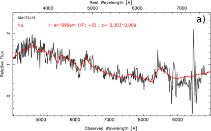
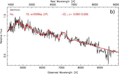
Supplementary Figure 1: Classification spectra of SNHiTS14B (a) and SNHITS14C (b) compared to SNID [11] templates.

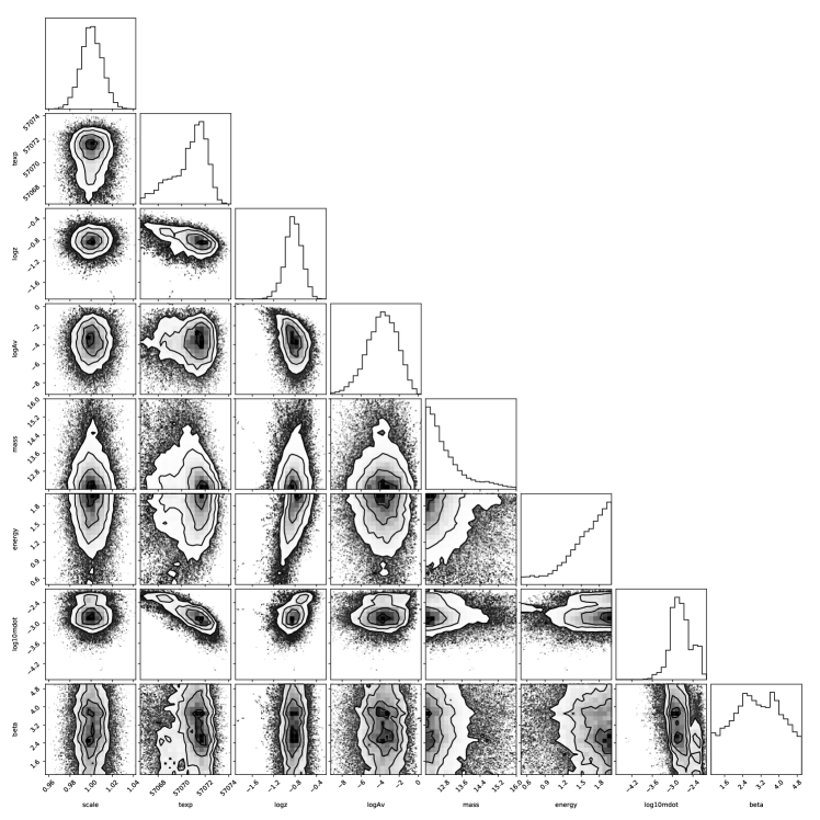
Supplementary Figure 2: Corner plot visualization of the posterior joint probability distribution of the parameters given the LC of Type II SN candidate SNHiTS15bc. The parameters used for this problem were a scale factor (forced to be close to one via a prior), the explosion time, the redshift $z$, the attenuation $A_{V}$, the main sequence mass, the energy of the explosion, the mass loss rate $\dot{M}$ and the wind acceleration parameter $\beta$. Note that $\dot{M}<10^{-4}$ $M_{\odot}$ yr^-1 are not favored for any combination of the other parameters.

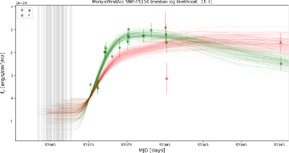
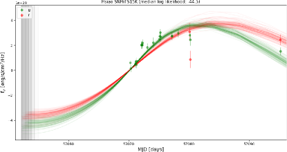
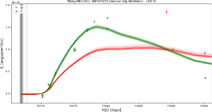
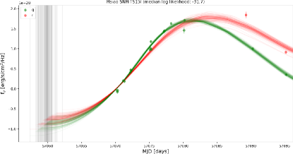
Supplementary Figure 3: Observations of SNHiTS15K (top row) and SNHiTS15I (bottom row) with models sampled from the posterior distribution of parameters for the RSG SN II models (left column) and SN I models (right column). SNHiTS15K is best fitted by a SN II model, with a median log–likelihood of -16.7 for the SN II model vs -44.5 for the SN I model; while SNHiTS15I is best fitted by a SN I model, with a median log–likelihood of -149 for the SN II model and -31.7 for the SN I model.

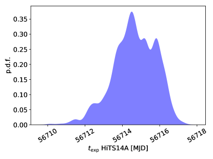
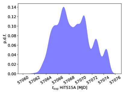
Supplementary Figure 4: Same as Figure 6, but for the distribution of median explosion times for the HiTS14A (l.h.s.) and HiTS15A (r.h.s.) campaigns.

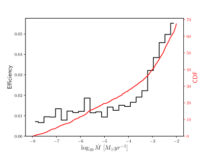
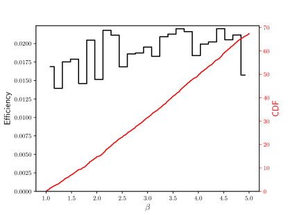
Supplementary Figure 5: Detection efficiency as a function of $\dot{M}$ and $\beta$ predicted by our simulations using a realistic distribution of redshifts and assuming the same depth and cadence as in our observations.

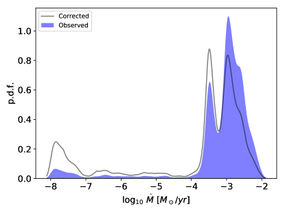
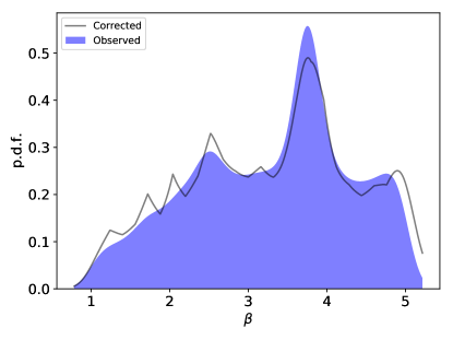
Supplementary Figure 6: Kernel density estimation of the sum of the sample posteriors marginalized over the mass loss rate $\dot{M}$ (l.h.s.) and wind acceleration parameter $\beta$ (r.h.s.) for the 26 SNe in the sample, using Silverman’s rule to estimate the kernel width. The density estimations are corrected by the detection efficiencies shown in Figure 5.

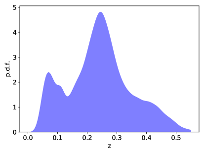
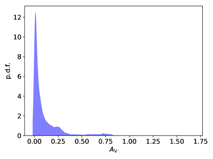
Supplementary Figure 7: Same as Figure 6, but for the distribution of redshift (l.h.s.) and attenuation (r.h.s.). Note that the apparent redshift bimodality is an artifact of the kernel density estimation. Using a Hartigans’ Dip test of Unimodality [17] with the inferred median redshift values we could not reject unimodality with a $p$–value of 0.84

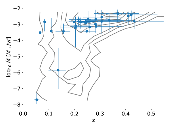
Supplementary Figure 8: Relation between inferred mass loss rate $\dot{M}$ and redshift for the sample of 26 early SNe II candidates from HiTS. The error bars correspond to the percentiles 5, 50 and 95 of the marginalized posterior distributions. We show for comparison the predicted distribution of $\log_{10}\dot{M}$ and redshift, as linearly spaced number density contours, in the case of a uniform distribution of $\log_{10}\dot{M}$ values (see text for more details).

Bibliography

- [1] Law, Nicholas M., et al., The Palomar Transient Factory: System Overview, Performance, and First Results. Publ. Astron. Soc. Pac., 121, 1395-1408 (2009).
- [2] Keller, S. C., et al., The SkyMapper Telescope and The Southern Sky Survey. Publ. Astron. Soc. Aus., 24, 1-12 (2007).
- [3] Kaiser, Nick, et al., The Pan-STARRS wide-field optical/NIR imaging survey. Soc. Phot. Inst. Eng., 7733, 77330E (2010).
- [4] Kim, Seung-Lee, et al., Wide-field telescope design for the KMTNet project. Soc. Phot. Inst. Eng., 8151, 81511B (2011).
- [5] Tonry, J. L., et al., ATLAS: A High-cadence All-sky Survey System. Publ. Astron. Soc. Pac., 130, 064505 (2018).
- [6] Flaugher, B., et al., The Dark Energy Camera. Astron. J., 150, 150 (2015).
- [7] Takada, Masahiro, Subaru Hyper Suprime-Cam Project. Proc. Am. Inst. Phys. Conf., 1279, 120 (2010).
- [8] Bellm, Eric & Kulkarni, Shrinivas The unblinking eye on the sky. Nat. Astron., 1, 0071 (2017).
- [9] LSST Science Collaboration, et al., Preprint at http://arxiv.org/abs/0912.0201 (2009).
- [10] Förster, F., et al., The High Cadence Transient Survey (HITS). I. Survey Design and Supernova Shock Breakout Constraints. Astrophys. J., 832, 155 (2016).
- [11] Smartt, S. J., Eldridge, J. J., Crockett, R. M., & Maund, J. R., The death of massive stars - I. Observational constraints on the progenitors of Type II-P supernovae. Mon. Not. R. Astron. Soc., 395, 1409 (2009).
- [12] Davies, Ben & Beasor, Emma R., The initial masses of the red supergiant progenitors to Type II supernovae. Mon. Not. R. Astron. Soc., 474, 2116 (2018).
- [13] Janka, Hans-Thomas, Melson, Tobias, & Summa, Alexander, Physics of Core-Collapse Supernovae in Three Dimensions: A Sneak Preview. Annu. Rev. Nucl. Phys., 66, 341 (2016).
- [14] Falk, S. W., Shock steepening and prompt thermal emission in supernovae. Astrophys. J., 225, L133 (1978).
- [15] Ensman, Lisa & Burrows, Adam, Shock breakout in SN 1987A. Astrophys. J., 393, 742 (1992).
- [16] Waxman, Eli & Katz, Boaz, Shock Breakout Theory, Handbook of Supernovae, 967 (2017).
- [17] Tominaga, N., et al., Shock Breakout in Type II Plateau Supernovae: Prospects for High-Redshift Supernova Surveys. Astrophys. J. Suppl. Ser., 193, 20 (2011).
- [18] Ofek, E. O., et al., Supernova PTF 09UJ: A Possible Shock Breakout from a Dense Circumstellar Wind. Astrophys. J., 724, 1396 (2010).
- [19] Gezari, S., et al., GALEX Detection of Shock Breakout in Type IIP Supernova PS1-13arp: Implications for the Progenitor Star Wind. Astrophys. J., 804, 28 (2015).
- [20] Moriya, Takashi J., Yoon, Sung-Chul, Gräfener, Götz, & Blinnikov, Sergei I., Immediate dense circumstellar environment of supernova progenitors caused by wind acceleration: its effect on supernova light curves. Mon. Not. R. Astron. Soc., 469, L108 (2017).
- [21] Moriya, Takashi J., Förster, Francisco, Yoon, Sung-Chul, Gräfener, Götz, & Blinnikov, Sergei I., Type IIP supernova light curves affected by the acceleration of red supergiant winds. Mon. Not. R. Astron. Soc., 476, 2840 (2018).
- [22] Yaron, O., et al., Confined dense circumstellar material surrounding a regular type II supernova. Nat. Phys., 13, 510 (2017).
- [23] Dessart, Luc, John Hillier, D., & Audit, Edouard, Explosion of red-supergiant stars: Influence of the atmospheric structure on shock breakout and early-time supernova radiation. Astron. Astrophys., 605, A83 (2017).
- [24] González-Gaitán, S., et al., The rise-time of Type II supernovae. Mon. Not. R. Astron. Soc., 451, 2212 (2015).
- [25] Rubin, Adam & Gal-Yam, Avishay, Unsupervised Clustering of Type II Supernova Light Curves. Astrophys. J., 828, 111 (2016).
- [26] Rubin, Adam & Gal-Yam, Avishay, Exploring the Efficacy and Limitations of Shock-cooling Models: New Analysis of Type II Supernovae Observed by the Kepler Mission. Astrophys. J., 848, 8 (2017).
- [27] Morozova, Viktoriya, Piro, Anthony L., & Valenti, Stefano, Unifying Type II Supernova Light Curves with Dense Circumstellar Material. Astrophys. J., 838, 28 (2017).
- [28] Schawinski, Kevin, et al., Supernova Shock Breakout from a Red Supergiant. Sci, 321, 223 (2008).
- [29] Gezari, Suvi, et al., Probing Shock Breakout with Serendipitous GALEX Detections of Two SNLS Type II-P Supernovae. Astrophys. J., 683, L131 (2008).
- [30] Garnavich, P. M., et al., Shock Breakout and Early Light Curves of Type II-P Supernovae Observed with Kepler. Astrophys. J., 820, 23 (2016).
- [31] Ganot, Noam, et al., The Detection Rate of Early UV Emission from Supernovae: A Dedicated Galex/PTF Survey and Calibrated Theoretical Estimates. Astrophys. J., 820, 57 (2016).
- [32] Tanaka, Masaomi, et al., Rapidly Rising Transients from the Subaru Hyper Suprime-Cam Transient Survey. Astrophys. J., 819, 5 (2016).
- [33] Bersten, M. C., et al., A surge of light at the birth of a supernova. Nat., 554, 497 (2018).
- [34] Smartt, S. J., et al., PESSTO: survey description and products from the first data release by the Public ESO Spectroscopic Survey of Transient Objects. Astron. Astrophys., 579, A40 (2015).
- [35] Lyman, J. D., et al., Bolometric light curves and explosion parameters of 38 stripped-envelope core-collapse supernovae. Mon. Not. R. Astron. Soc., 457, 328 (2016).
- [36] Hsiao, E. Y., et al., K-Corrections and Spectral Templates of Type Ia Supernovae. Astrophys. J., 663, 1187 (2007).
- [37] Quimby, Robert M., et al., SN 2006bp: Probing the Shock Breakout of a Type II-P Supernova. Astrophys. J., 666, 1093 (2007).
- [38] Paxton, Bill, et al., Modules for Experiments in Stellar Astrophysics (MESA). Astrophys. J. Suppl. Ser., 192, 3 (2011).
- [39] Paxton, Bill, et al., Modules for Experiments in Stellar Astrophysics (MESA): Planets, Oscillations, Rotation, and Massive Stars. Astrophys. J. Suppl. Ser., 208, 4 (2013).
- [40] Paxton, Bill, et al., Modules for Experiments in Stellar Astrophysics (MESA): Binaries, Pulsations, and Explosions. Astrophys. J. Suppl. Ser., 220, 15 (2015).
- [41] Puls, J., et al., O-star mass-loss and wind momentum rates in the Galaxy and the Magellanic Clouds Observations and theoretical predictions. Astron. Astrophys., 305, 171 (1996).
- [42] Bennett, P. D., Chromospheres and Winds of Red Supergiants: An Empirical Look at Outer Atmospheric Structure. ASPC, 425, 181 (2010).
- [43] Marshall, Jonathan R., et al., Asymptotic giant branch superwind speed at low metallicity. Mon. Not. R. Astron. Soc., 355, 1348 (2004).
- [44] Baade, Robert, et al., The Wind Outflow of zeta Aurigae: A Model Revision Using Hubble Space Telescope Spectra. Astrophys. J., 466, 979 (1996).
- [45] Mauron, N. & Josselin, E., The mass-loss rates of red supergiants and the de Jager prescription. Astron. Astrophys., 526, A156 (2011).
- [46] Goldman, Steven R., et al., The wind speeds, dust content, and mass-loss rates of evolved AGB and RSG stars at varying metallicity. Mon. Not. R. Astron. Soc., 465, 403 (2017).
- [47] Morozova, Viktoriya & Stone, James M., Theoretical X-ray light curves of young SNe II: the example of SN 2013ej. Preprint at http://arxiv.org/abs/1804.07312 (2018).
- [48] Blinnikov, S. I., Eastman, R., Bartunov, O. S., Popolitov, V. A., & Woosley, S. E., A Comparative Modeling of Supernova 1993J. Astrophys. J., 496, 454 (1998).
- [49] Blinnikov, Sergei, Lundqvist, Peter, Bartunov, Oleg, Nomoto, Ken’ichi, & Iwamoto, Koichi, Radiation Hydrodynamics of SN 1987A. I. Global Analysis of the Light Curve for the First 4 Months. Astrophys. J., 532, 1132 (2000).
- [50] Blinnikov, S. I., et al., Theoretical light curves for deflagration models of type Ia supernova. Astron. Astrophys., 453, 229 (2006).
- [51] Gal-Yam, Avishay, et al., A Wolf-Rayet-like progenitor of SN 2013cu from spectral observations of a stellar wind. Nat., 509, 471 (2014).
- [52] Groh, Jose H., Early-time spectra of supernovae and their precursor winds. The luminous blue variable/yellow hypergiant progenitor of SN 2013cu. Astron. Astrophys., 572, L11 (2014).
- [53] Gräfener, G. & Vink, J. S., Light-travel-time diagnostics in early supernova spectra: substantial mass-loss of the IIb progenitor of SN 2013cu through a superwind. Mon. Not. R. Astron. Soc., 455, 112 (2016).
- [54] Schroeder, K.-P., A study of ultraviolet spectra of Zeta Aurigae/VV Cephei systems. VII - Chromospheric density distribution and wind acceleration region. Astron. Astrophys., 147, 103 (1985).
- [55] Ohnaka, K., Weigelt, G., & Hofmann, K.-H., Vigorous atmospheric motion in the red supergiant star Antares. Nat., 548, 310 (2017).
- [56] Rodríguez, Ósmar, Clocchiatti, Alejandro, & Hamuy, Mario, Photospheric Magnitude Diagrams for Type II Supernovae: A Promising Tool to Compute Distances. Astron. J., 148, 107 (2014).

Bibliography

- [1] Walton, N., et al., PESSTO spectroscopic classification of optical transients. Astron. Tel., 5957, (2014).
- [2] Walton, N., et al., PESSTO spectroscopic classification of optical transients. Astron. Tel., 5970, (2014).
- [3] Le Guillou, L., et al., PESSTO spectroscopic classification of optical transients. Astron. Tel., 7144, (2015).
- [4] Baumont, S., et al., PESSTO spectroscopic classification of optical transients. Astron. Tel., 7154, (2015).
- [5] Forster, F., et al., Optical spectra of SNHiTS15al, SNHiTS15be, SNHiTS15bs and SNHiTS15by. Astron. Tel., 7291, (2015).
- [6] Pignata, G., et al., Optical spectroscopy of SNHiTS15aw. Astron. Tel., 7246, (2015).
- [7] Anderson, J., et al., Optical spectrosopy of SNHiTS15ad (Gabriela). Astron. Tel., 7164, (2015).
- [8] Anderson, J., et al., Optical spectrosopy of HiTS supernovae. Astron. Tel., 7335, (2015).
- [9] Anderson, J., et al., FORS2 spectroscopic classification of DECam SN candidates. Astron. Tel., 6014, (2014).
- [10] Anderson, J., et al., Optical spectrosopy of SNHiTS15D (Daniela) and SNHiTS15P (Rosemary). Astron. Tel., 7162, (2015).
- [11] Blondin, Stéphane & Tonry, John L., Determining the Type, Redshift, and Age of a Supernova Spectrum. Astrophys. J., 666, 1024 (2007).
- [12] Mighell, Kenneth John, CRBLASTER: A Parallel-Processing Computational Framework for Embarrassingly Parallel Image-Analysis Algorithms. Publ. Astron. Soc. Pac., 122, 1236 (2010).
- [13] Flewelling, H. A., et al., The Pan-STARRS1 Database and Data Products. Preprint at http://arxiv.org/abs/1612.05243 (2016).
- [14] Goodman, Jonathan & Weare, Jonathan, Ensemble samplers with affine invariance. Comm. Appl. Math. Comp. Sci., 5, 65 (2010).
- [15] Foreman-Mackey, Daniel, Hogg, David W., Lang, Dustin, & Goodman, Jonathan, emcee: The MCMC Hammer. Publ. Astron. Soc. Pac., 125, 306 (2013).
- [16] Silverman, B. W., Density estimation for statistics and data analysis. Mon. Stat. Appl. Prob. (1986).
- [17] J. A. Hartigan, P. M. Hartigan, The Dip Test of Unimodality. Ann. Statist., 13, 1, 70–84 (1985)