Probing ground-state phase transitions through quench dynamics

Abstract

The study of quantum phase transitions requires the preparation of a many-body system near its ground state, a challenging task for many experimental systems. The measurement of quench dynamics, on the other hand, is now a routine practice in most cold atom platforms. Here we show that quintessential ingredients of quantum phase transitions can be probed directly with quench dynamics in integrable and nearly integrable systems. As a paradigmatic example, we study global quench dynamics in a transverse-field Ising model with either short-range or long-range interactions. When the model is integrable, we discover a new dynamical critical point with a non-analytic signature in the short-range correlators. The location of the dynamical critical point matches that of the quantum critical point and can be identified using a finite-time scaling method. We extend this scaling picture to systems near integrability and demonstrate the continued existence of a dynamical critical point detectable at prethermal time scales. Therefore, our method can be used to approximately locate the quantum critical point. The scaling method is also relevant to experiments with finite time and system size, and our predictions are testable in near-term experiments with trapped ions and Rydberg atoms.

Introduction.—Experimental advances in isolating and controlling nonequilibrium quantum systems have brought within reach answers to many fundamental questions, including those related to thermalization, prethermalization, and many-body localization Deutsch (1991); Srednicki (1994, 1999); Rigol et al. (2008); Kim et al. (2014); Garrison and Grover (2018). The exquisite control of complex quantum systems has become commonplace as a result of progress in various platforms, such as trapped ions Richerme et al. (2014); Neyenhuis et al. (2017), ultracold atoms Kinoshita et al. (2006); Schreiber et al. (2015), nitrogen-vacancy centers Choi et al. (2017), Rydberg atoms Bernien et al. (2017), and others.

Among other interesting topics in nonequilibrium quantum many-body physics, phase transitions that emerge in the dynamics of isolated quantum systems have attracted significant theoretical and experimental interest Heyl et al. (2013); Žunkovič et al. (2018); Heyl (2018); Jurcevic et al. (2017); Zhang et al. (2017); Halimeh et al. (2017); Halimeh and Zauner-Stauber (2017); Homrighausen et al. (2017). There are two known types of dynamical phase transitions: (i) when a global order parameter (such as the Loschmidt echo) shows an abrupt change as a function of evolution time, or (ii) when a local order parameter measured after a sufficiently long time becomes nonanalytic as a function of some Hamiltonian parameter Žunkovič et al. (2018). This latter type of dynamical phase transition is closely related to quantum phase transitions; the only difference is that the order parameter is measured in the quenched state instead of the ground state. It is thus natural to ask how this dynamical phase transition is related to a quantum phase transition. While difficult to answer, this question is not only of fundamental importance, but also motivates the idea of using dynamics to study quantum phase transitions. In fact, in many of the above-mentioned experimental platforms, cooling a system to its ground state can be a formidable task while performing a quench experiment is now a routine practice.

In this Letter, we first establish a strong connection between the quantum critical point and a new dynamical critical point in a general class of integrable models, using the transverse-field Ising model (TFIM) as a paradigm. We show analytically that these critical points are identical and expect such behavior to generalize to other systems consisting of noninteracting particles Roy et al. (2017). This dynamical critical point has a nonanalytic signature in the long-time values of short-range, two-point correlation functions. Much of the previous work on the quench dynamics of the TFIM has focused on the behavior of long-range correlations Calabrese et al. (2011, 2012a, 2012b); Žunkovič et al. (2018); Halimeh et al. (2017); Karl et al. (2017), a common practice in studying equilibrium phase transitions. However, these correlations vanish in the thermodynamic limit for all nonzero field values due to the absence of long-range order at long time. Thus short-range correlations, often ignored due to the dominance of long-wavelength physics at low temperature, are important in identifying dynamical criticality and revealing its connections to quantum phase transitions.

Second, we show that analogous to the finite-size scaling analysis for identifying quantum critical points, one can perform a finite-time scaling analysis for obtaining the dynamical critical point. Intuitively, this can be understood because the evolution time controls the effective system size seen by short-range correlations as a result of emergent light cones. This finite-time scaling analysis is particularly favorable for quantum simulation experiments, as one does not need to create systems of different sizes or wait for a time much longer than the coherence time, and thus, allows for near-term experimental demonstration Zhang et al. (2017); Bernien et al. (2017).

Finally, we generalize our findings to systems that are nonintegrable by adding weak interactions. We show that the finite-time scaling predicts a dynamical critical point in the prethermal time scale. In general, the dynamical critical point will no longer coincide with the quantum critical point away from integrability. But, as shown by our analysis of the TFIM with next-nearest-neighbor and power-law decaying interactions, we expect the two transition points to be close to each other when interactions are weak. As perturbation theory may not work for finding quantum critical points of weakly interacting systems, our findings provide an alternative and experimental way of locating such critical points.

We point out that some earlier works have considered similar ideas of studying quantum criticality via quench dynamics. For example, Ref. Prosen (2000) studies the appearance of nonanalytic signatures in the periodically kicked Ising model, Ref. Roy et al. (2017) discusses nonanalytic signatures in the long-time dynamics in noninteracting topological phase transitions, and Ref. Heyl et al. (2018) uses out-of-time-order correlators (OTOCs) to identify quantum phase transitions. However, our approach offers three unique advantages: (i) The short-range correlations are easy to measure experimentally, especially compared to the OTOC. (ii) Our approach is not restricted to exactly integrable systems. (iii) The finite-time scaling analysis we introduce provides a method to locate the dynamical critical point.

Model.— We consider two models for the quench Hamiltonian of $L$ spins in one dimension: a transverse-field Ising model with either next-nearest-neighbor or long-range interactions,

$$H_{\text{NNN}} =-J\sum_{\langle i,j\rangle}\sigma_{i}^{x}\sigma_{j}^{x}-J\Delta\sum_{\langle\langle i,j\rangle\rangle}\sigma_{i}^{x}\sigma_{j}^{x}+B\sum_{i}\sigma_{i}^{z},$$ (1)

$$H_{\text{LR}} =-\sum_{i<j}J^{(\alpha)}_{ij}\sigma_{i}^{x}\sigma_{j}^{x}+B\sum_{i}\sigma_{i}^{z},$$ (2)

where $\{\sigma_{i}^{x,y,z}\}$ denote the Pauli matrices and $\langle\cdots\rangle$ and $\langle\langle\cdots\rangle\rangle$ denote nearest and next-nearest neighbors, respectively. We will use periodic boundary conditions to ensure translation invariance unless otherwise noted. In the long-range Hamiltonian, the Ising coupling is defined as $J^{(\alpha)}_{ij}=J\left[\frac{1}{\left|i-j\right|^{\alpha}}+\frac{1}{\left|L-(i-j)\right|^{\alpha}}\right]$, which accounts for periodic boundary conditions Sandvik (2003). We restrict to case of ferromagnetic interactions with $J$ and $\Delta>0$.

The quench and measurement protocol is shown schematically in Fig. 1(a). We initialize the system in a product state with all spins polarized in the Ising direction, $|\psi_{\rm in}\rangle=\ket{\rightarrow\cdots\rightarrow}$. This state is one of two degenerate ground states when $B=0$. We focus on the dynamics under the quench Hamiltonian [see Eqs. 1 and 2] of the nearest-neighbor, equal-time correlation function defined as

$$G(t)=\frac{1}{L}\sum_{\langle i,j\rangle}\langle\sigma^{x}_{i}(t)\sigma^{x}_{j}(t)\rangle_{\rm in},$$ (3)

where $\langle\cdots\rangle_{\rm in}$ indicates the expectation value with respect to the initial state $|\psi_{\rm in}\rangle$ defined above, and the operators are written in the Heisenberg picture, $\sigma^{x}_{i}(t)=e^{iHt}\sigma^{x}_{i}e^{-iHt}$. We note that the dynamics of two-point correlators at longer distances independent of the system size (e.g. $\langle\sigma_{i}^{x}\sigma_{i+2}^{x}\rangle$) will be similar to $G(t)$. However, calculating such longer range correlations would require a more complicated analytical treatment.

Results at the integrable point.—Consider first the nearest-neighbor TFIM [$\Delta=0$ in Eq. 1 or $\alpha=\infty$ in Eq. 2]. In this case, the Hamiltonian is integrable and can be mapped to free fermions via a Jordan-Wigner transformation with the boundary condition determined by the particle number parity sup . The quasiparticle dispersion is given by $\omega_{q}=2\sqrt{B^{2}-2BJ\cos q+J^{2}}$, where $q$ denotes momentum, and the Hamiltonian becomes $H=\sum_{q}\omega_{q}\gamma^{\dagger}_{q}\gamma_{q}$, where $\gamma_{q}$ are the annihilation operators for the Bogoliubov quasiparticles. The time evolution is governed by a set of conserved densities of these quasiparticles, $I_{q}=\gamma^{\dagger}_{q}\gamma_{q}$. The ground state of this model exhibits a second-order phase transition with the critical point at $B=B_{c}^{\rm gs}\equiv J$.

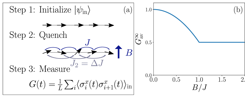
Figure 1: (a) Schematic picture of the quench. We evolve the initial state $|\psi_{\rm in}\rangle$, which consists of all spins polarized in the Ising direction, for a time $t$ under the Hamiltonian defined in Eq. 1 (shown) or Eq. 2. Then we measure the nearest-neighbor correlator $G(t)$ defined in Eq. 3. (b) The dependence of $G^{\infty}_{\rm av}$ on $B$ as given by Eq. 5.

We calculate the time-averaged correlator $G_{\text{av}}(t)\equiv\frac{1}{t}\int_{0}^{t}d\tilde{t}\,G(\tilde{t})$ to be sup

$$G_{\text{av}}(t)=\frac{1}{L}\sum_{q}\frac{8B^{2}}{\omega_{q}^{2}}\left[\left(\frac{J}{B}-\cos q\right)^{2}+j_{0}\left(2\omega_{q}t\right)\sin^{2}q\right],$$ (4)

where $j_{0}(z)=\sin\left(z\right)/z$ is a spherical Bessel function of the first kind. Note that the second term in the correlator decays at long times: $j_{0}\left(2\omega_{q}t\right)\rightarrow 0$ as $t\rightarrow\infty$ (the only exception being the $\omega_{q}=0$ case which contributes a time-independent constant $\propto 1/L$). This means that the first term in Eq. 4 corresponds to the long-time stationary value. Taking the thermodynamic limit, we obtain an analytic expression for $G_{\rm av}(t)$,

$$G^{\infty}_{\rm av} \equiv\lim_{\begin{smallmatrix}L\rightarrow\infty\\ t\rightarrow\infty\end{smallmatrix}}\frac{1}{t}\int_{0}^{t}d\tilde{t}\,G(\tilde{t})=\begin{cases}1-\frac{B^{2}}{2J^{2}}&\text{if }B\leq J\\ \frac{1}{2}&\text{if }B\geq J,\end{cases}$$ (5)

which has a nonanalyticity at $B=B_{c}^{\rm dy}\equiv J$. We refer to this nonanalytic point as a dynamical critical point. Note that the dynamical and ground state critical points are identical, $B_{c}^{\rm dy}=B_{c}^{\rm gs}$. This is because the nonanalyticity can be traced to the appearance of $1/\omega_{q}^{2}$ in the expression for $G_{\rm av}(t)$ [see Eq. 4], which has a pole at $B=B_{c}^{\rm gs}$. In Fig. 1(b), we plot the long-time value of the correlator $G^{\infty}_{\rm av}$ [Eq. 5], which exhibits a kink at $B=B_{c}^{\rm dy}$. Note that the expression for $G^{\infty}_{\rm av}$ is identical to that obtained from the Generalized Gibbs Ensemble (GGE) Vidmar and Rigol (2016) for the TFIM.

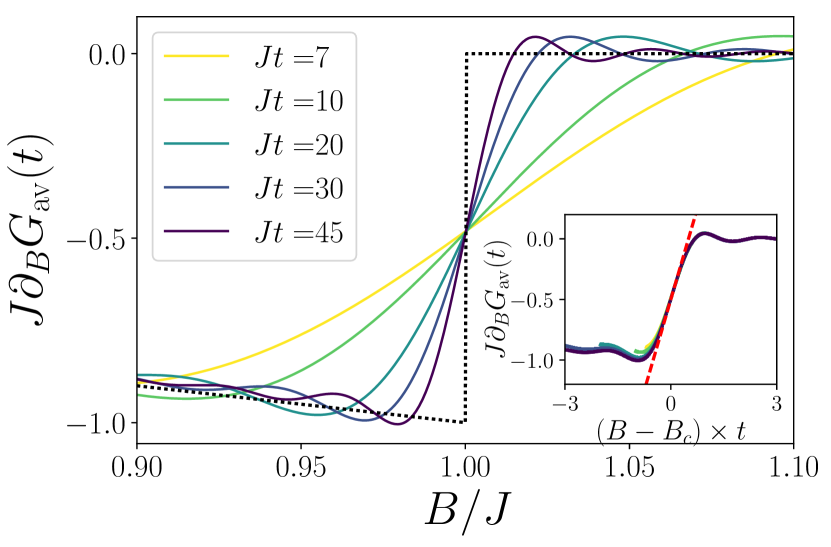
Figure 2: Finite-time scaling for the integrable case. The first derivative of the correlator, $\frac{\partial}{\partial B}G_{\rm av}(t)$, exhibits a sharper jump across the transition ($B=B_{c}^{\rm dy}=J$) at later times. The curves are obtained by differentiating Eq. 4 with a system size $L=100$ sup . The curves at different times cross at the same point, thus revealing a dynamical critical point. The dotted line in black indicates the expected discontinuity in the derivative in the thermodynamic limit ($L\rightarrow\infty$) and at long times ($Jt\rightarrow\infty$). (Inset) We extract the time dependence by performing a scaling collapse after rescaling the magnetic field $B$ by $t$. The scaling function near the critical point is linear, and is shown as a dashed red line.

The kink at the dynamical critical point is obtained after taking two limits in either order: (i) the infinite-time limit and (ii) the thermodynamic limit. In any realistic experiment, one can only measure $G_{\rm av}(t)$ at a finite time and a finite system size. In this case, $G_{\rm av}(t)$ is a smooth function of $B$, but we can nevertheless locate the dynamical critical point in the following way: We obtain the time-dependent derivative of $G_{\rm av}(t)$ with respect to $B$, i.e. $\partial_{B}G_{\rm av}(t)$ (see sup for the explicit expression), and plot it in Fig. 2. We find the curves at different times cross at the same point up to a small correction $\propto\frac{1}{L}$, thus revealing a dynamical critical point. In fact, all the curves can be made to collapse into a single curve (shown in the inset) by rescaling the field $B$ by $Jt$. The expression for the first derivative near the dynamical critical point takes the form of a universal scaling function, $\partial_{B}G_{\text{av}}(t)=\frac{1}{J}f((B-B_{c}^{\rm dy})t)$. To lowest order in the distance from the critical point (given by $\epsilon=B-B_{c}^{\rm dy}$), the scaling function is $f(\epsilon t)=-\frac{1}{2}+\epsilon t$ sup . Note that this finite-time scaling function is very similar to the finite-size scaling function of the long-time correlator near the critical point, with $t$ playing the role of $L/(3J)$ sup . The finite-time scaling analysis thus allows us to locate the position of the dynamical critical point, and in this (integrable) case, also the quantum critical point.

Let us discuss the generality of this result for different initial states. For an arbitrary initial state, $G^{\infty}_{\rm av}$ is given by

$$G^{\infty}_{\rm av,arbitrary}=\frac{1}{L}\sum_{q}\frac{2(J-B\cos q)}{\omega_{q}}\left[1-2\left\langle I_{q}\right\rangle_{\rm in}\right],$$ (6)

where $\left\langle I_{q}\right\rangle_{\rm in}$ is the expectation value of the conserved quasiparticle densities in the initial state. It is clear from this expression that the nonanalyticity which results from a gapless $\omega_{q}$ will survive for arbitrary initial states unless the form of $\left[1-2\left\langle I_{q}\right\rangle_{\rm in}\right]$ cancels off the $1/\omega_{q}$ singularity at $q=0$. A generic pure initial state, in particular a product state that can be easily prepared experimentally, will thus lead to the same dynamical critical behavior. Interestingly, a thermal initial state given by the density matrix $\rho_{\rm th}=e^{-\beta H}/\operatorname{tr}\left[e^{-\beta H}\right]$ is an exception. This is because in this case, $\langle I_{q}\rangle_{\rm in}=\operatorname{tr}(\rho_{\rm th}I_{q})=\frac{1}{2}\left[1-\tanh\left(\frac{\beta\omega_{q}}{2}\right)\right]\approx\frac{1}{2}\left(1-\frac{\beta}{2}\omega_{q}\right)$ when $\omega_{q}\rightarrow 0$ and thus $G^{\infty}_{\rm av}$ becomes an analytic function of $B$. This is consistent with the well-known fact that the 1D nearest-neighbor TFIM does not have a thermal phase transition.

Results away from integrability.—Now, let us consider the TFIM with either an additional next-nearest-neighbor interaction [$\Delta\neq 0$ in Eq. 1] or long-range interactions [any finite $\alpha$ in Eq. 2]. Assuming the Eigenstate Thermalization Hypothesis (ETH) Srednicki (1999) holds, we expect local observables, including $G(t)$, to thermalize at sufficiently long times. For any finite value of $\Delta$ or $\alpha>2$, it has been established that the TFIM does not exhibit a thermal phase transition Sachdev (2011); Dutta and Bhattacharjee (2001). Thus, once the system fully thermalizes, any measured observable has to be analytic and thus, it should no longer have a dynamical critical point. (The situation with $\alpha<2$ is beyond the scope of this Letter due to the strong effects of long-range interactions that could break ETH Žunkovič et al. (2018).)

However, as recently shown by Refs. Halimeh et al. (2017); Halimeh and Zauner-Stauber (2017), it is possible to still observe a dynamical phase transition when local observables have not yet thermalized but instead have reached prethermal values. This is the case here when $\Delta$ is small or $\alpha$ is large, so that the Hamiltonian is nearly integrable and prethermalization is expected to occur Mori et al. (2018); Langen et al. (2016). The dynamical critical point in the prethermal regime is also relevant for experiments in the near future, as the thermalization timescale is likely to be far beyond the experimental coherence time Neyenhuis et al. (2017); Kinoshita et al. (2006); Gring et al. (2012).

We now show that our finite-time scaling method can also reveal a dynamical critical point in the prethermal regime of a nearly integrable system. We calculate the non-integrable dynamics numerically due to the lack of analytic solutions. Using a split-operator decomposition (using fourth-order Suzuki-Trotter expansion) coupled with a Walsh-Hadamard transform, we calculate dynamics for up to $L=25$ spins (see sup for technical details). In Figs. 3(a) and (b) we plot the time dependence of the derivative of $G_{\rm av}(t)$ for $\Delta=0.1$ and $\alpha=6$ respectively. Remarkably, the curves at different times still cross at one point, which we identify as the dynamical critical point $B_{c}^{\rm dy}$. These curves will also collapse almost perfectly on top of each other using a scaling function $\partial_{B}G_{\rm av}(t)=\frac{1}{J}\tilde{f}\left((B-B_{c}^{\rm dy})t\right)$ sup , similar to the integrable case.

In the integrable TFIM, we showed that the dynamical critical point $B_{c}^{\rm dy}$ coincides with the ground-state critical point $B_{c}^{\rm gs}$. It is natural to ask whether this is still the case for the above-calculated models near integrability. To locate the quantum critical point, we compute the Binder cumulant Binder (1981), $\mathcal{U}^{\rm gs}_{4}=1-\frac{\langle M^{4}\rangle_{\rm gs}}{3\langle M^{2}\rangle^{2}_{\rm gs}}$ (where $M=\frac{1}{L}\sum_{i}\sigma^{x}_{i}$ and $\langle\cdots\rangle_{\rm gs}$ denotes the ground-state expectation value) using a DMRG algorithm for a system with open boundary conditions and sizes ranging from $L=30$ to $L=140$. We identify the quantum critical point using a finite-size scaling method as shown in Figs. 3(c) and (d). It is found that $B_{c}^{\rm dy}$ is close, but not identical, to $B_{c}^{\rm gs}$ at both $\Delta=0.1$ and $\alpha=6$.

While we cannot make a conclusive statement about whether $B_{c}^{\rm dy}$ agrees with $B_{c}^{\rm gs}$ in the thermodynamic limit based on finite-size numerical calculations, we argue that $B_{c}^{\rm dy}$ and $B_{c}^{\rm gs}$ should in general be different but close to each other when near integrability. To support this argument, we perform a self-consistent mean-field calculation Sen and Chakrabarti (1991) for Eq. 1 with $\Delta=0.1$ to identify both $B_{c}^{\rm dy}$ and $B_{c}^{\rm gs}$ in the thermodynamic limit sup . The next-nearest-neighbor spin interaction translates to a perturbative two-particle interaction of the Jordan-Wigner fermions. The essence of the self-consistent calculation is to approximate this interaction by effective single-particle hoppings and on-site energies. This makes the Hamiltonian noninteracting, with the quench dynamics given by an effective GGE. The parameters of this effective Hamiltonian must be determined self-consistently from the expectation values of different correlation functions. These expectation values may be considered either in the ground state or the effective GGE corresponding to the quench from some initial state. While the former determines the quantum critical point $B_{c}^{\rm gs}$ Sen and Chakrabarti (1991), we claim that the latter captures the dynamical critical point $B_{c}^{\rm dy}$. Therefore, it is natural to expect a difference in the locations of the dynamical and quantum critical points.

The self-consistent mean-field calculation should be asymptotically exact as $\Delta\rightarrow 0$. We find that to first order in $\Delta$, $B^{\rm dy}_{c}\approx J\left(1+\frac{3}{2}\Delta\right)$ and $B^{\rm gs}_{c}\approx J\left(1+\frac{16}{3\pi}\Delta\right)$ sup . For $\Delta=0.1$, these predict $B_{c}^{\rm dy}\approx 1.15$ and $B_{c}^{\rm gs}\approx 1.168$, agreeing very well with numerics in Figs. 3(a) and (c). We have further confirmed the accuracy of these predictions for $\Delta$ up to 0.3 sup . For the larger values of $\Delta$, it is clear that $B^{\rm dy}_{c}\neq B^{\rm gs}_{c}$, but they are close in magnitude when $\Delta\approx 0$.

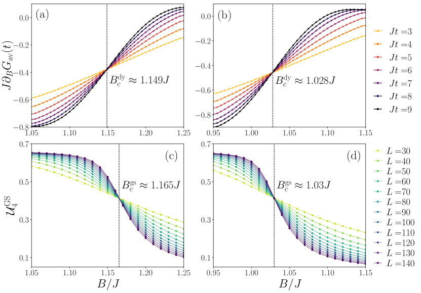
Figure 3: Comparison between the finite-time scaling of the time-averaged nearest-neighbor correlator $G_{\rm av}(t)$ and the ground-state Binder cumulant $\mathcal{U}_{4}^{\rm gs}$. The first column [panels (a) and (c)] corresponds to the TFIM with next-nearest-neighbor interaction $\Delta=0.1$ [Eq. 1], while the second column [panels (b) and (d)] corresponds to the TFIM with long-range interaction $\alpha=6$ [Eq. 2]. The finite-time scaling of the quench dynamics is shown in the first row, and the finite-size scaling for the ground state is shown in the second row. The dynamical critical points ($B_{c}^{\rm dy}$) identified in (a) and (b) using finite-time scaling are close but different from the locations of the quantum critical points ($B_{c}^{\rm gs}$) identified in (c) and (d). The ground-state simulations were done using a DMRG algorithm with bond dimension $\chi=32$.

Discussion.—Our results are relevant to experiments in trapped ions Zhang et al. (2017) and Rydberg atoms Bernien et al. (2017), where dynamics of the TFIM can be readily probed. As an example, we numerically obtain the dynamics for the $\alpha=6$ TFIM, which models Rydberg atoms interacting via van der Waals type long-range interactions Saffman et al. (2010). We find that the numerically obtained dynamical critical point $B^{\rm dy}_{c}\approx 1.028J$ shown in Fig. 3(b) is very close to the ground-state critical point $B^{\rm gs}_{c}\approx 1.03J$ obtained from finite-size scaling shown in Fig. 3(d). We emphasize that the dynamical critical point is identified by our finite-time scaling method for a system size of only 25 spins and an evolution time of only $9/J$, which are well within the current experimental record for the system size and coherence time Bernien et al. (2017). As a result, we believe our method can be used in near-future experiments to identify critical points of quantum phase transitions using quench dynamics.

Our work opens up several interesting questions for future consideration: (i) How should one classify the observed dynamical critical point? We note that the dynamical critical point identified using $G(t)$ as an “order parameter” does not represent a conventional symmetry-breaking phase transition, because for both $B<B_{c}^{\rm dy}$ and $B>B_{c}^{\rm dy}$, the quenched state does not spontaneously break the Ising symmetry and become ferromagnetically ordered. (ii) Is finite-time scaling a general method for identifying dynamical critical points? We believe that for generic, short-range interacting systems, finite-time scaling serves the purpose of finite-size scaling for finding the quantum critical point due to the emergence of linear light cones Lieb and Robinson (1972). However, when interactions become long-range, the linear light cone may no longer exist Foss-Feig et al. (2015); Eldredge et al. (2017) and it remains unclear when the finite-time scaling method fails. (iii) Could the link between dynamical and quantum critical points established here be generalized to other integrable and nearly integrable systems, such as systems solvable by Bethe ansatz or many-body localized systems? Here the link is provided by the single-particle spectrum that governs both equilibrium and nonequilibrium physics, but what happens when the single-particle spectrum is less relevant? (iv) Could there be similar links between dynamical phase transitions and phase transitions in excited eigenstates? This is particularly relevant in many-body localized systems Huse et al. (2013). (v) Can the prethermal dynamical critical point be predicted using other theoretical methods such as the kinetic equations using time-dependent GGEs D’Alessio et al. (2016); Bertini et al. (2015) or Keldysh field theory?

in 1,…,6 See pages \x of dpt-supp