An improved Lieb-Robinson bound for many-body Hamiltonians with power-law interactions

Abstract

In this work, we prove a new family of Lieb-Robinson bounds for lattice spin systems with long-range interactions. Our results apply for arbitrary $k$-body interactions, so long as they decay with a power-law greater than $kd$, where $d$ is the dimension of the system. More precisely, we require that the sum of the norm of terms with diameter greater than or equal to $R$, acting on any one site, decays as a power-law $1/R^{\alpha}$, with $\alpha>d$. These new bounds allow us to prove that, at any fixed time, the spatial decay of quantum information follows arbitrarily closely to $1/r^{\alpha}$. Moreover, we define a new light-cone for power-law interacting quantum systems, which captures the region of the system where changing the Hamiltonian can affect the evolution of a local operator. In short-range interacting systems, this light-cone agrees with the conventional definition. However, in long-range interacting systems, our definition yields a stricter light-cone, which is more relevant in most physical contexts.

In a relativistic quantum field theory, information can never travel faster than the speed of light. A Lieb-Robinson bound Lieb and Robinson (1972); Nachtergaele and Sims (2006); Hastings and Koma (2006); Nachtergaele and Sims (2009); Nachtergaele et al. (2009); Nachtergaele and Sims (2010) establishes a similar “light-cone” for the spread of quantum information in a non-relativistic lattice system. However, the information spread outside the light-cone is not strictly vanishing but, instead, has non-zero tails. Such constraints on the spread of information, in addition to being physically important in their own right, have also been used as ingredients in the rigorous mathematical proof of key results about non-relativistic lattice systems Hastings (2004); Nachtergaele and Sims (2006); Hastings and Wen (2005); Hastings and Koma (2006); Osborne (2007); Nachtergaele and Sims (2007); Bravyi et al. (2006); Hastings (2007); Bravyi et al. (2010); Bravyi and Hastings (2011); Bachmann et al. (2012); Michalakis and Zwolak (2013); Abanin et al. (2017), including the exponential decay of correlations in the ground states of gapped Hamiltonians Nachtergaele and Sims (2006); Hastings and Koma (2006) and the stability of topological order Bravyi et al. (2006, 2010); Bravyi and Hastings (2011); Michalakis and Zwolak (2013).

More recently, new results have generalized Lieb-Robinson bounds to lattice spin systems with interactions between distant spins that fall off as a power of their separation Hastings and Koma (2006); Hauke and Tagliacozzo (2013); Eisert et al. (2013); Richerme et al. (2014); Foss-Feig et al. (2015); Matsuta et al. (2017). Such long-range interactions arise in a wide variety of experimental platforms, ranging from solid-state spin defects Ruderman and Kittel (1954); Kasuya (1956); Yosida (1957) to quantum optical systems of trapped ions Blatt and Roos (2012), polar molecules Moses et al. (2017), and Rydberg atoms Saffman et al. (2010). While the majority of previous studies have focused on few-body physics, recent advances have enabled a number of these platforms to begin probing the many-body dynamics and information propagation of strongly interacting, long-range systems Yan et al. (2013); Richerme et al. (2014); Zeiher et al. (2017).

Motivated by the development of these physical platforms, in this work, we improve Lieb-Robinson bounds for generic power-law interactions. Specifically, let us consider a system of spins on a lattice $\Lambda$ governed by a Hamiltonian $H$, which can be written as a sum $H=\sum_{Z}H_{Z}$ of terms acting on sets of lattice sites $Z\subseteq\Lambda$ in $d$-dimensional space. Moreover, we assume (among other conditions described in Section I) that there exists a constant $J$ such that

$$\sup_{z\in\Lambda}\sum_{Z\ni z:\mathrm{diam}(Z)\geq R}||{H_{Z}}||\,\,\leq\,\,\frac{J}{R^{\alpha}},$$ (1)

where $\mathrm{diam}(Z)$ is the greatest distance between any two points in $Z$. A familiar example Zhang et al. (2017); Choi et al. (2017) is the long-range Ising interaction,

$$H=H_{\text{short-range}}+J\sum_{i\neq j}\frac{1}{|\textbf{r}_{i}-\textbf{r}_{j}|^{d+\alpha}}\sigma_{i}^{z}\sigma_{j}^{z}.$$ (2)

An early result on Lieb-Robinson bounds in power-law interacting systems was proved in Ref. Hastings and Koma (2006), which demonstrated the existence of a light-cone whose size grows exponentially in time for any $\alpha>0$. More recently, this result was improved in Refs. Foss-Feig et al. (2015) and Matsuta et al. (2017), where it was shown that a power-law light-cone emerges for $\alpha>d$, where $d$ is the spatial dimension.

However, each of these results has certain limitations (Table I). On the one hand, Ref. Foss-Feig et al. (2015) assumes a two-body Hamiltonian, where each term acts on at most two spins.  This assumption limits the usage of this result in analyzing multi-body effective Hamiltonians of broad interest in condensed matter physics. Such Hamiltonians can arise in a number of different contexts: for example, ring-exchange interactions may be important in solid ³He Thouless (1965) and are known to stabilize certain topological phases Misguich et al. (1999); Paramekanti et al. (2002); multi-body Hamiltonians arise in explicit constructions of various results in mathematical physics Hastings and Wen (2005); Bravyi et al. (2010); Bravyi and Hastings (2011); Abanin et al. (2017); and higher-body interactions naturally emerge in the effective description of periodically-driven two-body Hamiltonians Bukov et al. (2015); Abanin et al. (2017).

Reference	Multi-body Hamiltonians	Asymptotic Spatial Decay	LC1	LC2
Foss-Feig et al. Ref. Foss-Feig et al. (2015)	✗	$r^{-(\alpha+d)}$	$\alpha>d$	$\alpha>d$
Matsuta et al. Ref. Matsuta et al. (2017)	✓	$r^{-(\alpha-d)/(\eta+1)}$	$\alpha>d$	$\alpha>2d$
Present work	✓	$r^{-\alpha}$	$\alpha>d$	$\alpha>d$

Table 1: Summary of power-law Lieb-Robinson bounds for $\alpha>d$. Note that the LC1 and LC2 columns describe the power-law regime where these light-cones exist and are power-law.

On the other hand, while Ref. Matsuta et al. (2017) overcomes this two-body assumption, it proves a significantly weaker result regarding the power-law decay of information outside the light-cone (Table I). In particular, for $\alpha\gtrsim d$, the bounds of Ref. Matsuta et al. (2017) ensure only a relatively slow decay outside the light-cone; which can limit its applicability to some important results, e.g. bounding the difference in operators time evolved under slightly different Hamiltonians.

In this paper, we prove a Lieb-Robinson bound that addresses both of the above concerns. We demonstrate that for multi-body interactions with $\alpha>d$, the spatial decay of quantum information outside the light-cone scales arbitrarily closely to $\sim 1/r^{\alpha}$ (Table I). While this bound is not as strong as the $\sim 1/r^{\alpha+d}$ decay obtained in Ref. Foss-Feig et al. (2015), our combination of an improved scaling (over Ref. Matsuta et al. (2017)) and applicability to arbitrary multi-body Hamiltonians, enables the usage of this Lieb-Robinson bound to prove new results in mathematical physics Machado et al. (prep).

An important comment is in order. Unlike either short-range or exponentially decaying interactions, power-law interactions are characterized by Lieb-Robinson bounds with power-law tails which lack a natural notion of a length scale. This implies that one should be particularly careful when defining an associated light-cone for such long-range interacting systems. One possible definition of a light-cone (used in Refs. Foss-Feig et al. (2015); Matsuta et al. (2017)) is the following: at late times, outside the light-cone, the propagated quantum information is small. From here on, we will refer to this as light-cone 1 (LC1). For short-range interacting systems, LC1 is the only length-scale associated with time evolution. For power-law interacting systems, one can already get a sense of the insufficiency of LC1 by noting the following: despite the fact that the asymptotic spatial decays obtained in Refs. Foss-Feig et al. (2015), Matsuta et al. (2017) and this work are quite different (Table I), they all yield the same LC1 (Table II).

To this end, we introduce a second light-cone, LC2, which properly captures these differences. In particular, LC2 ensures that at late times, the evolution of the operator is not affected by changes to the Hamiltonian outside of LC2. For short-range interacting systems, LC1 and LC2 coincide, but for long-range interacting systems, they can be quite different. More specifically, Ref. Foss-Feig et al. (2015) exhibits a finite, power-law LC2 for $\alpha>d$, while Ref. Matsuta et al. (2017) does not have a finite LC2 for $\alpha<2d$, despite both having the same power-law LC1. Intuitively, the lack of an LC2 for $\alpha>d$ in Ref. Matsuta et al. (2017) is due to the aforementioned slow asymptotic spatial decay of quantum information. This highlights the importance of our improved decay; it enables us to prove our second main result, which is the existence of a power-law LC2 for $\alpha>d$ for arbitrary multi-body Hamiltonians (Table I).

I Assumptions and notation

Our notation will be similar to that of Ref. Matsuta et al. (2017). We consider a set of lattice sites $\Lambda$ with a metric $d(x,y)$ for $x,y\in\Lambda$, and a Hamiltonian $H$ written as a sum of terms $H=\sum_{Z}H_{Z}$, where $H_{Z}$ is supported on the set $Z\subseteq\Lambda$. We extend the notation of the metric to sets, denoting $d(X,Y)$ as the minimum distance between any two elements of the sets $X,Y\subseteq\Lambda$, as well as between sets and sites, denoting $d(X,y)=d(X,\{y\})$. We define a function $f(R)$ that captures the power-law decay of interactions:

$$f(R):=\sup_{z\in\Lambda}\sum_{Z\ni z:\mathrm{diam}(Z)\geq R}\|H_{Z}\|~{},$$ (3)

where

$$\mathrm{diam}(Z)=\sup_{x,y\in Z}d(x,y)~{},$$ (4)

and we assume there are constants $J$ and $\alpha>d$ (the dimensionality of the system) such that $f(R)\leq JR^{-\alpha}$. We also require that the sum of the operator norms of all of the terms involving any site be finite:

$$\mathcal{C}_{0}:=\sup_{x\in\Lambda}\sum_{y\in\Lambda}\sum_{Z\ni x,y}\|H_{Z}\|<\infty~{}.$$ (5)

Finally, we assume certain regularity conditions on the lattice $\Lambda$. Specifically, we assume that $\Lambda$ can be embedded in Euclidean space $\mathbb{R}^{d}$, so that for each $z\in\Lambda$ there is a corresponding $\textbf{r}_{z}\in\mathbb{R}^{d}$, such that $d(x,y)=|\mathbf{r}_{x}-\mathbf{r}_{y}|$. Moreover, we assume there is a smallest lattice separation $a$ such that $d(x,y)\geq a$ for any $x,y\in\Lambda$ unless $x=y$. We choose to work in units such that $a=1$.

Let us also define $\tau_{t}^{H}(O)$ as the operator $O$ time-evolved according to the Heisenberg representation

$$\tau_{t}^{H}(O)=e^{itH}\,O\,e^{-itH}.$$ (6)

Throughout the paper we will use “$C$” to refer to any constants that depends only on $\sigma$ (the parameter introduced in the statement of the theorem in the next section) and the lattice. It will not necessarily be the same constant each time it appears.

II Main result

Theorem 1.

Given the assumptions stated in Section I, let observables $A$ and $B$ be supported on sets $X$ and $Y$ respectively. Then for any $(d+1)/(\alpha+1)<\sigma<1$:

$$\|[\tau_{t}^{H}(A),B]\|\leq\|A\|\|B\|\left\{2|X|e^{vt-r^{1-\sigma}}+C_{1}\frac{\mathfrak{G}(vt)}{r^{\sigma\alpha}}\right\},$$ (7)

where $r=d(X,Y)$ and $v=C_{2}\max\{J,\mathcal{C}_{0}\}$. Moreover, there exists a constant $C_{3}$ such that:

$$\mathfrak{G}(\tau)\leq C_{3}(\tau+\tau^{1+d/(1-\sigma)})|X|^{n^{*}+2},$$ (8)

where

$$n^{*}=\left\lceil\frac{\sigma d}{\sigma\alpha-d}\right\rceil$$ (9)

Here, all $C_{i}$ are constants only dependent on $\sigma$ and the lattice.

By choosing $\sigma$ arbitrarily close to $1$ we obtain a decay of the Lieb-Robinson bound that approaches $\sim r^{-\alpha}$ for large $r$.

III Proof

III.1 Iteration Procedure

The main challenge in understanding the spread of quantum information in long-range interacting systems is being able to differentiate the contribution from strong “short” range terms and the weak “long” range terms in a problem with no natural length scale. As a result, there is no single separation between “short” and “long” range terms of the Hamiltonian that yields a strict bound. We develop a construction that iteratively introduces a new short scale, enabling us to improve on the Lieb-Robinson bound by better accounting for the spatial decay of interactions in the Hamiltonian.

As a starting point, we consider a truncated version of our long-range Hamiltionian with a cutoff $R$, $H^{\leq R}$:

$$H^{\leq R}\,\, =\sum_{Z:\mathrm{diam}(Z)\leq R}H_{Z}~{}.$$ (10)

At the end of our construction we can make $R\to\infty$, recovering the full Hamiltonian. Because $H^{\leq R}$ has finite range $R$, a Lieb-Robinson bound for short-ranged Hamiltonians can be applied. However, this is clearly not the optimal bound, as it assumes all interactions of range up to $R$ are equally strong, ignoring their decay with range. Nevertheless, this provides the starting point for our iterative process.

At each iteration, the Hamiltonian $H^{\leq R}$ is split into a short and a long-range piece using a cutoff $R^{\prime}$:

$$H^{\leq R}=H^{\leq R^{\prime}}+H^{R^{\prime};R}\quad\text{where}\quad H^{R^{\prime};R}=\sum_{Z:R^{\prime}<\mathrm{diam}(Z)\leq R}H_{Z}.$$ (11)

Then, following the strategy of Refs. Foss-Feig et al. (2015) and Matsuta et al. (2017), the time-evolution of an operator $A$ is separated into a contribution from the short-range part $H^{\leq R^{\prime}}$ and the long-range part $H^{R^{\prime};R}$; these play the role, respectively, of the unperturbed Hamiltonian and the perturbation in the interaction representation.

Then, using Lemma 3.1 in Ref. Matsuta et al. (2017), we can bound the total spread of the operator as a contribution from the short-range part $H^{\leq R^{\prime}}$, as well as an additional contribution due to the long-range part $H^{R^{\prime};R}$:

$$\|[\tau_{t}^{H^{\leq R}}(A),B]\|\leq\|[\tau_{t}^{H^{\leq R^{\prime}}}(A),B]\|+2\|B\|\int_{0}^{t}\|[\tau_{t-s}^{H^{\leq R^{\prime}}}(A),H^{R^{\prime};R}]\|~{}ds$$ (12)

This procedure enables us to better distinguish the contribution of the strong short-range terms and the weak long-range terms of the evolution, improving upon the initial naive bound. Once an improvement is obtained, one can perform the procedure again further reducing the contribution from the long-range piece of Eq. (12) and improving the spatial decay of the Lieb-Robinson bound. We note this iterative process recovers the argument of Ref. Matsuta et al. (2017) after one iteration; by iterating multiple times we can improve on their results. We make this iterative construction more precise with the following Lemma:

Lemma 1.

Fix a set $X\subseteq\Lambda$ and a time $t$. Suppose that we have a function $\lambda^{(R)}(r)$ such that for all $0\leq s\leq t$, $Y\subseteq\Lambda$ and observables $A$ and $B$ supported on sets $X$ and $Y$ respectively, the bound

$$\|[\tau_{s}^{H^{\leq R}}(A),B]\|\leq\lambda^{(R)}(d(X,Y))\|A\|\|B\|$$ (13)

is satisfied. We assume that $\lambda^{(R)}(r)$ is monotonically increasing in $R$ and decreasing in $r$. Then, for any $R^{\prime}>0$, Eq. (13) is also satisfied with $\lambda$ replaced by $\widetilde{\lambda}$, defined according to

$$\widetilde{\lambda}^{(R)}(r)=\lambda^{(R^{\prime})}(r)+C\Theta(R-R^{\prime})\,|X|\,t\,f(R^{\prime})\,\mathcal{I}[\lambda^{(R^{\prime})}],$$ (14)

where $f(R)$ is given in Eq. (3); $C$ is a constant independent of $R,R^{\prime},|X|$ and $t$; $\Theta(x)$ is the Heaviside theta function and:

$$\mathcal{I}[\lambda]=\lambda(0)+\int_{1/2}^{\infty}\rho^{d-1}\lambda(\rho)~{}d\rho.$$ (15)

Proof.

For $R^{\prime}\geq R$, the result follows directly from the monotonicity with respect to $R$. On the other hand, for $R^{\prime}<R$ we have, from Eq. (12):

$$\|[\tau_{t}^{H^{\leq R}}(A),B]\| \leq\|[\tau_{t}^{H^{\leq R^{\prime}}}(A),B]\|+2\|B\|\int_{0}^{t}\|[\tau_{t-s}^{H^{\leq R^{\prime}}}(A),H^{R^{\prime};R}]\|\,ds$$ (16)

$$\leq\|[\tau_{t}^{H^{\leq R^{\prime}}}(A),B]\|+2\|B\|\int_{0}^{t}\sum_{Z:R^{\prime}<\mathrm{diam}(Z)\leq R}\|\bigl{[}\tau_{s}^{H^{\leq R^{\prime}}}(A),H_{Z}\bigr{]}\|\,ds$$ (17)

$$\leq\lambda^{(R^{\prime})}(d(X,Y))\|A\|\|B\|+2t\|B\|\!\!\!\!\sum_{Z:R^{\prime}<\mathrm{diam}(Z)\leq R}\lambda^{(R^{\prime})}(d(X,Z))\|H_{Z}\|\|A\|$$ (18)

$$\leq\lambda^{(R^{\prime})}(d(X,Y))\|A\|\|B\|+2t\|A\|\|B\|\sum_{z\in\Lambda}~{}\sum_{Z\ni z:R^{\prime}<\mathrm{diam}(Z)\leq R}\lambda^{(R^{\prime})}(d(X,z))\|H_{Z}\|$$ (19)

$$\leq\lambda^{(R^{\prime})}(d(X,Y))\|A\|\|B\|+2t\|A\|\|B\|f(R^{\prime})\sum_{z\in\Lambda}\lambda^{(R^{\prime})}(d(X,z))$$ (20)

$$\leq\|A\|\|B\|\left\{\lambda^{(R^{\prime})}(d(X,Y))+2tf(R^{\prime})|X|\sup_{x\in X}\sum_{z\in\Lambda}\lambda^{(R^{\prime})}(d(x,z))\right\}.$$ (21)

In going from the second line to the third line, it is helpful to recall that $\lambda^{(R^{\prime})}(d(X,Y))$ is independent of $s$ (but dependent on $t$). In going from the fourth line to the fifth, we used:

$$\sum_{z\in\Lambda}\sum_{Z\ni z,R^{\prime}<\mathrm{diam}(Z)<R}\lambda^{(R^{\prime})}(d(X,z))\|H_{Z}\| =\sum_{z\in\Lambda}\lambda^{(R^{\prime})}(d(X,z))\sum_{Z\ni z,R^{\prime}<\mathrm{diam}(Z)<R}\|H_{Z}\|$$ (23)

$$\leq f(R^{\prime})\sum_{z\in\Lambda}\lambda^{(R^{\prime})}(d(X,z)).$$ (24)

To get the final result, we use Lemma 2 from the Appendix to replace the sum by an integral in the last line of Eq. (LABEL:eqn:recursion).

Finally, let us note that the simplest bound for $\lambda^{(R^{\prime})}(d(X,Y))$ corresponds to the short-range Lieb-Robinson bound where the interactions have at most range $R^{\prime}$. ∎

We now iteratively apply Lemma 1. Eq. (14) says that a Lieb-Robinson bound $\lambda^{(R)}$ for an interaction with maximum range $R$ can be rewritten as the sum of two contributions: a Lieb-Robinson bound $\lambda^{(R^{\prime})}$ for an interaction of maximum range $R^{\prime}$, which can be interpreted as the “short-range part of the evolution”; and an additional propagation of quantum information due to “long-range hops”, which have range between $R^{\prime}$ and $R$ and maximum strength $f(R^{\prime})$. However, these “long-range hops” need not originate in the support of the original $A$ itself but, rather, in the support of the time-evolved $A$ under the short-range part of the interaction. The latter spreads the quantum information by ${\mathcal{I}}[\lambda^{(R’)}]$, as depicted in Fig. 1.

At each iteration we replace the short-range contribution by the short-range Lieb-Robinson bound. We make use of the bound proven in Theorem A.1 of Ref. Matsuta et al. (2017) which state that, for observables $A$ and $B$ supported on sets $X$ and $Y$, respectively:

$$\|[\tau_{t}^{H^{\leq R^{\prime}}}(A),B]\|\leq 2|X|\exp[vt-d(X,Y)/R^{\prime}]\|A\|\|B\|~{}.$$ (25)

Finally, we are free to choose $R^{\prime}$ in Eq. (14) so we take it to be a function of $r$; specifically, at the $n$-th iteration we take $R^{\prime}=r^{\sigma_{n}}$, with $d/\alpha<\sigma_{n}<1$. The resulting bound no longer depends on any cut-off $R^{\prime}$ and when used again in Eq. (14), leads to a faster decaying $\mathcal{I}[\lambda]$ and an improved bound.

Therefore, at the $n$-th iteration we obtain the bound:

$$\|[\tau_{s}^{H^{\leq R}}(A),B]\|\leq\lambda^{(R)}_{n}(d(X,Y))\|A\|\|B\|,$$ (26)

where the iteration equation is:

$$\lambda^{(R)}_{n}(r)=\Delta_{r\,}\left(2|X|\exp\left[vt-r^{1-\sigma_{n}}\right]+C\Theta(R-r^{\sigma_{n}})|X|t\,f(r^{\sigma_{n}})\mathcal{I}[\lambda_{n-1}^{(r^{\sigma_{n}})}]\right),$$ (27)

where

$$\Delta_{r\,}\!(u)=\begin{cases}2&r<1~{}\mathrm{or}~{}u>2\\ u&\mathrm{otherwise}\end{cases}$$ (28)

This choice of $\Delta_{r}$ ensures that we always use the trivial bound on the commutator when $r=0$ or when it is the most stringent bound. Now, it only remains to carry out the iteration.

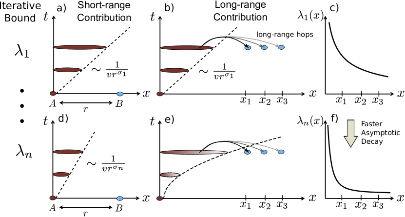
Figure 1: The Lieb-Robinson bound measures the spread of quantum information during evolution by bounding the commutator of a time evolved local operator $A$, with another operator $B$ a distance $r$ away. The spread the operator $A$ can be apportioned into the spread due to interactions of range shorter than $R^{\prime}$ (left column) and long-range hops due to interactions of range larger than $R^{\prime}$ (center column). The long-range hops connect the short-range time evolved operator $A$ with strength at most $f(R^{\prime})$ but they can originate from any location that $A$ has spread to, so the total contribution of these long-range hops is weighted by the integral $\mathcal{I}[\lambda]$ (see Lemma 1). At the first iterative step, which yields $\lambda_{1}$, the short-range interactions can always be characterized by an exponentially decaying bound with a sharp light-cone with slope $(vR^{\prime})^{-1}$, Eq. (25). This corresponds exactly to the short-range contribution to $\lambda_{1}$ (a). The long-range contribution arises from the long-range hops that connect the inside of the light-cone to the support of $B$ (b). By choosing the cut-off $R^{\prime}$ as a function of the operator distance, $R^{\prime}=r^{\sigma_{1}}$, the resulting bound becomes the sum of exponential and power-law decaying terms, Eq. (32), the latter of which dominate the long distance decay of the bound (c). This choice of $R^{\prime}$ leads to the light-cone slope of $(vr^{\sigma_{1}})^{-1}$ of panel (a). At the $n$-th iteration step, which yields $\lambda_{n}$, we choose a new cut-off $\tilde{R}^{\prime}$. As before, we obtain a short-range contribution that yields a linear light-cone with slope $(v\tilde{R}^{\prime})^{-1}$ (d). More importantly, the long-range hops will now be weighted by the power-law decay of the previous bound $\lambda_{n-1}$, illustrated by the red shading (e). It is the combination of these two power-law decays that enables our iterative procedure to improve the asymptotic decay of the bound $\lambda_{n}$ after specifying the cut-off as $\tilde{R}^{\prime}=r^{\sigma_{n}}$ (f) (see Section III.B). This choice of $\tilde{R}^{\prime}$ leads to the light-cone slope of $(vr^{\sigma_{n}})^{-1}$ of panel (d).

III.2 Analyzing the iteration

To begin the iterative process we can invoke the generic Lieb-Robinson bound for finite-range Hamiltonians, as described in Eq. (25). Taking into account the trivial case,

$$\|[\tau_{t}^{H^{\leq R}}(A),B]\|\leq 2\|A\|\|B\|,$$ (29)

we begin the iteration with the initial bound:

$$\lambda_{0}^{(R)}(r)=\Delta_{r}(2|X|e^{vt-r/R}).$$ (30)

We then find (calculation in Appendix B.1):

$$\mathcal{I}[\lambda_{0}^{(R^{\prime})}]\leq C|X|\Bigl{[}1+(vtR^{\prime})^{d}\Bigr{]}$$ (31)

Taking Eq. (27) and setting $R^{\prime}=r^{\sigma_{1}}$, we have:

$$\lambda_{1}^{(R)}(r)\leq\Delta_{r\,\,}\!\!\Bigl{(}2|X|e^{vt-r^{1-\sigma_{1}}}+C\Theta\bigl{(}R-r^{\sigma_{1}}\bigr{)}\,|X|^{2}Jtr^{-\sigma_{1}\alpha}[1+r^{\sigma_{1}d}(vt)^{d}]\Bigr{)}$$ (32)

which recovers the results in Ref. Matsuta et al. (2017) with an appropriate choice of $\sigma_{1}$. From this point, we proceed by induction. Indeed, suppose at the $n$-th iteration we have:

$$\lambda_{n}^{(R)}(r)\leq\Delta_{r\,\,}\!\!\Bigl{(}2|X|e^{vt-r^{1-\sigma_{n}}}+\,C\Theta(R-r^{\sigma_{n}})\sum_{i=1}^{2}\mathfrak{F}^{(n)}_{i}(vt)\,r^{\mu^{(n)}_{i}}\Bigr{)}.$$ (33)

Note that, according to Eq. (32), this is satisfied for $n=1$ if we take

$$\mu^{(1)}_{1} =\sigma_{1}(-\alpha+d)$$ (34)

$$\mu^{(1)}_{2} =-\sigma_{1}\alpha$$ (35)

$$\mathfrak{F}^{(1)}_{1}(\tau) =C\tau^{d+1}|X|^{2}$$ (36)

$$\mathfrak{F}^{(1)}_{2}(\tau) =C\tau|X|^{2}$$ (37)

Then, so long as $\mu_{1}^{(n)}+d>0$ and $\mu_{2}^{(n)}+d<0$ we have (as computed in Appendix B.2):

$$\mathcal{I}[\lambda_{n}^{(R^{\prime})}]\leq C\left[\left\{|X|(1+(vt)^{d/(1-\sigma_{n})})+\mathfrak{F}_{2}^{(n)}(vt)~{}(vt)^{(d+\mu_{2}^{(n)})/(1-\sigma_{n})}\right\}+\mathfrak{F}^{(n)}_{1}(vt)~{}(R^{\prime})^{(\mu^{(n)}_{1}+d)/\sigma_{n}}\right]$$ (38)

and therefore, using Eq. (27) and setting $R^{\prime}=r^{\sigma_{n+1}}$:

$$\lambda_{n+1}^{(R)}(r)\leq\Delta_{r\,}\!\Bigl{(}2|X|e^{vt-r^{1-\sigma_{n+1}}}+~{}$$

$$+C\Theta(R-r^{\sigma_{n+1}})|X|Jtr^{-\sigma_{n+1}(\alpha-(\mu^{(n)}_{1}+d)/\sigma_{n})}~{}\mathfrak{F}^{(n)}_{1}(vt)+$$

$$+C\Theta(R-r^{\sigma_{n+1}})|X|Jtr^{-\sigma_{n+1}\alpha}\left\{|X|(1+(vt)^{d/(1-\sigma_{n})})+\mathfrak{F}_{2}^{(n)}(vt)~{}(vt)^{(d+\mu_{2}^{(n)})/(1-\sigma_{n})}\right\}~{}.$$ (39)

By choosing $\sigma_{n+1}\leq\sigma_{n}$ we ensure that the spatial decay of the exponential term does not increase in performing the iterative procedure.

So at the next iteration we have

$$\mu^{(n+1)}_{1} =\sigma_{n+1}\bigl{(}-\alpha+(\mu^{(n)}_{1}+d)/\sigma_{n}\bigr{)}$$ (40)

$$\mu^{(n+1)}_{2} =-\sigma_{n+1}\alpha$$ (41)

$$\mathfrak{F}_{1}^{(n+1)}(\tau) =C\tau|X|~{}\mathfrak{F}_{1}^{(n)}(\tau)$$ (42)

$$\mathfrak{F}_{2}^{(n+1)}(\tau) =C\tau|X|\left\{|X|[1+\tau^{d/(1-\sigma_{n})}]+\mathfrak{F}_{2}^{(n)}(\tau)~{}\tau^{(d+\mu_{2}^{(n)})/(1-\sigma_{n})}\right\}$$ (43)

Iteratively applying Eq. (40) to the initial condition of Eq. (34) yields:

$$\mu^{(n)}_{1}=\left(1+\frac{1}{\sigma_{1}}+\frac{1}{\sigma_{2}}+\ldots\frac{1}{\sigma_{n-1}}\right){\sigma_{n}}d\,-\,n{\sigma_{n}}\alpha.$$ (44)

At each iteration, $\mu_{1}^{(n)}$ is made smaller (i.e. more negative) at the cost of increasing the leading power of $\tau$ in $\mathfrak{F}_{1}^{(n)}(\tau)$, so long as $\mu^{(n)}_{1}>-d$. By choosing appropriate $\sigma_{j}$, we eventually reach an iteration step $n=n^{*}$ such that $\mu_{1}^{(n^{*})}+d<0$ and Eq. (38) no longer holds (and neither will the iteration equations Eqs. (40) - (43)). For $n>n^{*}$, $\mathcal{I}[\lambda^{R^{\prime}}_{n}]$ becomes independent of $R^{\prime}$:

$$\mathcal{I}[\lambda_{n\geq n^{*}}^{R^{\prime}}]\leq C\left[|X|(1+(vt)^{d/(1-\sigma_{n})})+\mathfrak{F}_{1}^{(n)}(vt)~{}(vt)^{(d+\mu^{(n)}_{1})/(1-\sigma_{n})}+\mathfrak{F}_{2}^{(n)}(vt)~{}(vt)^{(d+\mu^{(n)}_{2})/(1-\sigma_{n})}\right]$$ (45)

which leads to new iterative steps where the spatial decay of both polynomial terms is the same:

$$\mu^{(n+1)}_{1} =\mu^{(n+1)}_{2}=-\sigma_{n+1}\alpha$$ (46)

$$\mathfrak{F}_{1}^{(n+1)}(\tau) =\tau^{1+(d+\mu_{1}^{(n)})/(1-\sigma_{n})}|X|~{}\mathfrak{F}_{1}^{(n)}(\tau)$$ (47)

$$\mathfrak{F}_{2}^{(n+1)}(\tau) =\tau|X|\left\{|X|[1+\tau^{d/(1-\sigma_{n})}]+\mathfrak{F}_{2}^{(n)}(\tau)\tau^{(d+\mu_{2}^{(n)})/(1-\sigma_{n})}\right\}~{}.$$ (48)

At this point in the iterative procedure, further iterations do not improve on the power-law decay of the Lieb-Robinson bound since they are set by $-\sigma_{n}\alpha$.

With regards to the time dependence of the bound, at each iteration step $n$, one can choose $\sigma_{n}>(1-\sigma_{n-1}+d)/\alpha$, reducing the time dependence of $\mathfrak{F}_{i}^{(n)}(vt)$ in Eqs. (43), (47) and (48). For such choices of $\sigma_{n}$ and enough iterations steps, the leading temporal dependence arises from the $\tau^{1+d/(1-\sigma_{n})}$ term introduced each iteration step in Eq. (48). As a result, there is some iteration number $m>n^{*}$ above which the most meaningful terms of the bound do not change. At this point, the bound $\lambda^{(R)}_{m}(r)$ is given by:

$$\lambda^{(R)}_{m}\leq\Delta_{r}\left(2|X|e^{vt-r^{1-\sigma_{1}}}+C\Theta(R-r^{\sigma_{m}})r^{-\sigma_{m}\alpha}\left\{|X|^{2}(vt)^{1+d/(1-\sigma_{1})}+\ldots\right\}\right)~{},$$ (49)

where $\ldots$ are terms with lower power in $vt$, but higher power in $|X|$.

We can make the previous considerations more concrete by analyzing the case where $\sigma_{j}$ are all made equal, $\sigma_{j}=\sigma>(d+1)/(\alpha+1)$. This inequality ensures the reduction of the time dependence of $\mathfrak{F}^{(n)}_{i}(vt)$.

For this choice of $\{\sigma_{j}\}$, Eq. (44) simplifies to:

$$\mu^{(n)}_{1}=(n-1+\sigma)d-n\sigma\alpha$$ (50)

further leading to $n^{*}=\lceil\sigma d/(\sigma\alpha-d)\rceil$.

For $n>n^{*}$, the time dependence is encoded in:

$$\mathfrak{F}_{1}^{(n)}(\tau) \sim\tau^{1+d/(1-\sigma)}\left[\tau^{[1+d-\sigma(1+\alpha)]/[1-\sigma]}\right]^{n-1}+\ldots$$ (51)

$$\mathfrak{F}_{2}^{(n)}(\tau) \sim\tau^{1+d/(1-\sigma)}+\ldots$$ (52)

where $\ldots$ correspond to lower power of $\tau$. Then, $\mathfrak{F}_{2}(\tau)$ becomes the dominant term immediately for iteration step $n^{*}+1$ as the term $[~{}\cdot~{}]^{n-1}$ reduces the leading term of $\mathfrak{F}_{1}^{(n)}(\tau)$ to be smaller than $\mathfrak{F}_{2}^{(n)}(\tau)$. Because different terms have different dependences on $|X|$, to ensure all constants are independent of $|X|$, we include the largest power of $|X|$ emmerging from our construction in front of the time dependence. Finally, taking $R\to\infty$ yields the final result as expressed in Theorem 1.

IV Power-law light-cones

In short-range interacting systems, the length scale associated with the exponential decay of the Lieb-Robinson bound, Eq. (25), provides a natural definition for a light-cone. In contrast, Lieb-Robinson bounds in long-range interacting systems are characterized by power-law decays that lack a natural length scale. As a result, the precise notion of a light-cone will vary depending on which properties we wish to capture.

One way to define a light-cone is in terms of the “spread of information”: that is, suppose we consider the time evolution of two states $|\psi\rangle$ and $O|\psi\rangle$, where $O$ is a local operator that perturbs the initial state. The light-cone is the region of radius $R_{\mathrm{LC1}}(t)$ around the support of $O$, outside which, both time-evolved states yield nearly identical local observables. It is a direct measure of the spread of the influence of the perturbation $O$ across the system as a function of time $t$. We refer to this light-cone as LC1.

A different way to define a light-cone is in terms of the region of the system that can affect the evolution of local observables appreciably. More specifically, consider the time evolution of an operator $O$ under two different Hamiltonians, $H$ and $H+\Delta H$. Intuitively, if $\Delta H$ only acts very far away from $O$, it will not have a significant impact on the evolution of $O$ at short times. One can make this intuition precise and guarantee that the evolution of $O$ does not change appreciably, until time $t$, if $\Delta H$ only acts a distance $R_{\mathrm{LC2}}(t)$ away from $O$. $R_{\mathrm{LC2}}(t)$ then characterizes the “zone of influence” of the evolution of operator $O$. We refer to this light-cone as LC2. Strictly speaking, LC2 is not a light-cone. However, this “zone of influence” is intimately connected with a modified notion of the past light-cone. Our usual understanding of such a past light-cone consists of all events (points in space-time) where acting with a local operator can influence the current event. The modified past light-cone that is naturally associated with LC2 corresponds to all events where a change in the Hamiltonian can influence the current event. In long-range systems, these two light-cones need not be equal, as even a local change to the Hamiltonian can affect the system non-locally.

In general, in power-law interacting systems, LC2 will be greater than LC1. Intuitively, as the operator $O$ expands outwards, the number of terms of $\Delta H$ it can interact with increases dramatically. As a result, it is not only necessary that the operator is mostly localized to a particular region, but also that the spatial profile of the operator spread decays fast enough to counteract the increasing number of terms that can modify its dynamics.

We now make these definitions more precise. In order to simplify the notation in this section, we write the Lieb-Robinson bound between two operators $A$ and $B$, such that $d(A,B)=r$, as:

$$\frac{\|[\tau^{H}_{t}(A),B]\|}{\|A\|\|B\|}\leq\mathcal{C}(r,t),$$ (53)

This allows us to formally define LC1 as the light-cone used in the previous literature:

Definition 1.

Let light-cone 1 (LC1) be defined as a relation $r=f(t)$ such that:

$$\lim_{t\to\infty}\mathcal{C}(f(t),t)=0.$$ (54)

The meaning of LC1 is that the propagation of quantum information outside the light-cone is small and gets smaller as $t\rightarrow\infty$ . Because we are interested in the asymptotic behavior, we focus on power-law light-cones, $f(t)=t^{\gamma}$, which characterize the Lieb-Robinson bounds considered here. The smallest light-cone is characterized by the exponent $\beta^{\mathrm{LC1}}$, the infimum of the $\gamma$ which satisfy Eq. (54).

In contrast we wish to define LC2 as the region outside which changing the Hamiltonian of the system has no significant impact in the evolution of the operator. To obtain a precise condition for LC2, we consider how changing the Hamiltonian $H$ to $H+\Delta H$ impacts the evolution of an operator. More specifically, we consider modifying the Hamiltonian only a distance $r_{min}$ away from the operator of interest $O$. In Appendix C, we show the difference in the time evolved operators is bounded by:

$$\|e^{iHt}Oe^{-iHt}-e^{i(H+\Delta H)t}Oe^{-i(H+\Delta H)t}\|\leq C\Delta J\|O\|t\int_{r_{min}}^{\infty}dr~{}r^{d-1}\mathcal{C}(r,t)$$ (55)

where $\Delta J$ quantifies the difference between the Hamiltonians.

LC2 is then given by the relationship between $r_{min}$ and $t$ that ensures that operator difference, bound in Eq. (55), remains small and goes to zero in the long time limit. This immediately motivates the definition of LC2 as follows:

Definition 2.

Let light-cone 2 (LC2) be defined as a relation $r=f(t)$ such that:

$$\lim_{t\to\infty}\quad t\int_{f(t)}^{\infty}dr~{}r^{d-1}\mathcal{C}(r,t)=0,$$ (56)

where $d$ is the dimensionality of the system.

Again, we will focus on polynomial light-cones, $f(t)=t^{\gamma}$ and define $\beta^{\mathrm{LC2}}$ as the infimum of the $\gamma$ which satisfy Eq. (56).

In short-ranged interacting systems, where $\mathcal{C}(r,t)\propto e^{vt-r/R}$, the exponential suppression of $\mathcal{C}(r,t)$ at large $r$ is insensitive to the extra volume term in the definition of LC2, Eq. (56), leading to the same linear light-cone for both LC1 and LC2. This result is an immediate consequence of the natural length scale in $\mathcal{C}(r,t)$.

However, in long-range interacting systems, $\mathcal{C}(r,t)$ has a power-law decay which is sensitive to the extra volume term in LC2. For example, for Eq. (56) to converge and ensure a power-law LC2, the Lieb-Robinson bound must decay faster than $r^{-d}$; for LC1 there is no such requirement. As a result, for slowly-decaying Lieb-Robinson bounds one may have a power-law LC1 but no LC2, i.e. there is no power-law $f(t)$ that satisfies Eq. (56). This is the case for the bound in Matsuta et al. Matsuta et al. (2017), where LC2 does not exist for $d<\alpha<2d$, yet LC1 matches that of Foss-Feig et al. Foss-Feig et al. (2015). LC2 is able to capture the difference between these two results.

By comparison, our result supports both an LC1 and LC2 for $d<\alpha$, extending the existence of an LC2 in long-range multi-spin Hamiltonians to $d<\alpha<2d$. In this regime both our Lieb-Robinson bound and that of Ref. Foss-Feig et al. (2015) lead to finite LC2, albeit with a larger light-cone exponent for our bound. Much like the difference in decay profile, this might be inherent to our treatment of the more general case of arbitrary multi-spin interactions.

In Table 2 and Figure 2, we compare the different light-cone exponents obtained from both our work and previous literature for different values of $\alpha$. In Figure 2, we plot the exponent of LC2 of the different works as a function of $\alpha$ for dimension $d=1$. More details on the calculation, and the general formulae for all space dimensions $d$, can be found in Appendix D.

Reference	LC1 $(d<\alpha)$	LC2 $(d<\alpha\leq 2d)$	LC2 $\left(2d<\alpha<\alpha_{M}\right)$	LC2 $\left(\alpha_{M}\leq\alpha\right)$
Ref. Foss-Feig et al. (2015)	$\beta^{\mathrm{LC1}}_{\text{FF}}=\dfrac{\alpha+1}{\alpha-d}$	$\beta^{\mathrm{\mathrm{LC2}}}_{\text{FF}}=\dfrac{\alpha+d}{\alpha}\dfrac{\alpha+1}{\alpha-d}+\dfrac{1}{\alpha}$	$\beta^{\mathrm{LC2}}_{\text{FF}}=\dfrac{\alpha+d}{\alpha}\dfrac{\alpha+1}{\alpha-d}+\dfrac{1}{\alpha}$	$\beta^{\mathrm{LC2}}_{\text{FF}}=\dfrac{\alpha+d}{\alpha}\dfrac{\alpha+1}{\alpha-d}+\dfrac{1}{\alpha}$
Ref. Matsuta et al. (2017)	$\beta^{\mathrm{LC1}}_{\text{M}}=\dfrac{\alpha+1}{\alpha-d}$	✗	$\beta^{\mathrm{LC2}}_{\text{M}}=\dfrac{\alpha+2}{\alpha-2d}$	$\beta^{\mathrm{LC2}}_{\text{M}}=\dfrac{\alpha+2}{\alpha-2d}$
Present Work	$\beta^{\mathrm{LC1}}=\dfrac{\alpha+1}{\alpha-d}$	$\beta_{\text{FF}}^{\mathrm{LC2}}<\beta^{\mathrm{LC2}}=\tilde{\beta}$	$\beta_{\text{FF}}^{\mathrm{LC2}}<\beta^{\mathrm{LC2}}=\tilde{\beta}<\beta^{\mathrm{LC2}}_{\text{M}}$	$\beta^{\mathrm{LC2}}=\dfrac{\alpha+2}{\alpha-2d}$

Table 2: Summary of the power-law light-cone exponents of LC1 and LC2 for both previous literature and our work. We use the subscript FF and M to refer to the light-cone exponents from the bounds of Refs. Foss-Feig et al. (2015) and Matsuta et al. (2017) respectively. Here $\tilde{\beta}=\frac{2}{(\alpha-d)^{2}}\times\left[\alpha-d+\alpha d(1+\sqrt{1+2/d-2/\alpha})\right]$ and $\alpha_{M}=\frac{3d}{2}\left[1+\sqrt{1+\frac{8}{9d}}\right]$. For a detailed calculation see Appendix D.

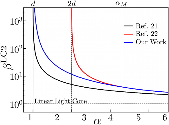
Figure 2: Power-law LC2 exponent for the present paper and Refs. Foss-Feig et al. (2015) and Matsuta et al. (2017) for $d=1$ as a function of $\alpha$. While Ref. Matsuta et al. (2017) has a finite power-law LC2 for $\alpha>2d$, Ref. Foss-Feig et al. (2015) and our work have a power-law LC2 for all $\alpha>d$. For $\alpha<\alpha_{M}$ our work leads to a better LC2 than Ref. Matsuta et al. (2017), while matching it for $\alpha\geq\alpha_{M}$. The horizontal dashed line corresponds to a linear light-cone. More details about the calculation can be found in Appendix D.

V Discussion

In this paper, we have proven an improved Lieb-Robinson bound for generic multi-body long-range interactions, characterized by a faster asymptotic spatial decay. The importance of this improvement is captured by the notion of LC2, a definition of light-cone that provides a stricter definition of locality for the growth of operators, in particular, that their evolution is not affected by the outside region for large $t$. Our work extends the existence of an LC2 light-cone for generic multi-body interacting systems for $d<\alpha<2d$.

This improvement has important implications for understanding prethermalization and Floquet phases of matter in periodically-driven systems. In such systems (especially in the high frequency regime), one can capture the evolution under a time-dependent Hamiltonian $H(t)$ using a time-independent approximation. Even when the original $H(t)$ has strictly two-body terms, the time-independent approximation will naturally exhibit multi-body terms. The results which establish the accuracy and limitations of such approximations require Lieb-Robinson bounds for multi-body power-law interactions with a rapid decay outside the light-cone. This application will be discussed in future work Machado et al. (prep).

During the preparation of this manuscript, the authors became aware of a new Lieb-Robinson bound Tran et al. (2018) that improves upon Ref. Foss-Feig et al. (2015). The bound in Ref. Tran et al. (2018) has an LC1 exponent of $\alpha/(\alpha-d)$ under similar assumptions as Ref. Foss-Feig et al. (2015), namely, two-body interactions. However, their result (phrased in terms of commutators) does not yield a finite LC2 for $d<\alpha<2d$. Nevertheless, the structure of their arguments is intriguing and understanding how to generalize their results to multi-body interactions is a promising direction for future study.

Appendix A Some technical results

Lemma 2.

Let $f(r)$ be a monotonically decreasing function of $r$, and fix an $x\in\Lambda$. Then

$$\sum_{z\in\Lambda,a\leq d(z,x)\leq R}f(d(z,x))\leq\frac{C}{a^{d}}\int_{a/2}^{R}f(r)r^{d-1}~{}dr,$$ (57)

where $a$ is the minimum separation between lattice points.

Proof.

Around each lattice point $z$, consider a ball $B_{z}$ of radius $a/2$. Given our assumption that $a$ is the smallest separation between lattice points, these balls are pairwise disjoint (up to sets of measure zero). Now, for any r in $B_{z}$, we have that $f(|\textbf{r}-\textbf{r}_{x}|-a/2)\geq f(d(z,x))$. Therefore,

$$Vf(d(z,x))\leq\int_{B_{z}}f(|\textbf{r}-\textbf{r}_{x}|-a/2)~{}d^{d}\textbf{r},$$ (58)

where $V$ is the volume of the ball $B_{z}$. In the case that $d(x,z)<3a/2$, we will use the tighter bound

$$Vf(d(z,x))\leq\int_{B_{z}:|\textbf{r}-\textbf{r}_{x}|<a}f(|\textbf{r}-\textbf{r}_{x}|)~{}d^{d}\textbf{r}+\int_{B_{z}:|\textbf{r}-\textbf{r}_{x}|>a}f(|\textbf{r}-\textbf{r}_{x}|-a/2)~{}d^{d}\textbf{r},$$ (59)

Now using the fact that $\cup B_{z}\subseteq\mathbb{R}^{d}$, we find that

$$\sum_{z\in\Lambda:a\leq d(z,x)\leq R}f(d(z,x)) \leq\frac{C}{a^{d}}\left(\int_{a/2}^{a}r^{d-1}f(r)~{}dr+\int_{a}^{R+a/2}r^{d-1}f(r-a/2)~{}dr\right).$$ (60)

We can bound the second integral by

$$\int_{a}^{R+a/2}r^{d-1}f(r-a/2)~{}dr =\int_{a/2}^{R}(u+a/2)^{d-1}f(u)~{}du$$ (61)

$$\leq C^{\prime}\int_{a/2}^{R}u^{d-1}f(u)~{}du.$$ (62)

This immediately proves the Lemma.

∎

Lemma 3.

For any $\mu$ and $\nu$ and positive $\rho$ then the following inequality holds for a constant $C$ independent of $\rho$:

$$\int_{\rho}^{\infty}e^{-x^{\nu}}x^{\mu}~{}dx\leq Ce^{-\rho^{\nu}}\left(1+\rho^{\mu-\nu+1}\right)$$ (63)

Proof.

It sufficient to consider the case of $\nu=1$, since we can reduce to this case by a change of variables. Let us first consider $\mu<0$, then:

$$\int_{\rho}^{\infty}e^{-x}x^{\mu}~{}dx\leq\rho^{\mu}\int_{\rho}^{\infty}e^{-x}~{}dx =\rho^{\mu}e^{-\rho}$$ (64)

We are now left with the case $\mu>0$. In that case, if $\rho\leq 1$ then we can certainly bound the left-hand side of Eq. (63) by:

$$\int_{\rho}^{\infty}e^{-x}x^{\mu}~{}dx\leq e^{1-\rho}\left[\int_{0}^{\infty}e^{-x}x^{\mu}\right]=C_{1}e^{-\rho}.$$ (65)

On the other hand, for $\rho\geq 1$, we have

$$\int_{\rho}^{\infty}e^{-x}x^{\mu}~{}dx =e^{-\rho}\rho^{\mu}\int_{\rho}^{\infty}e^{-(x-\rho)}(x/\rho)^{\mu}~{}dx$$ (66)

$$=e^{-\rho}\rho^{\mu}\int_{0}^{\infty}e^{-u}(u/\rho+1)^{\mu}~{}du$$ (67)

$$\leq e^{-\rho}\rho^{\mu}\int_{0}^{\infty}(u+1)^{\mu}e^{-u}~{}du$$ (68)

$$=C_{2}e^{-\rho}\rho^{\mu}\leq C_{2}e^{-\rho}\rho^{\mu+\epsilon},$$ (69)

for any $\epsilon>0$. Adding both bounds with $C=\max(C_{1},C_{2})$ ensures it holds for all values of $\rho$. ∎

Appendix B Calculation of $\mathcal{I}[\lambda]$

In this Appendix we perform the calculation of short-range spread of quantum information $\mathcal{I}[\lambda^{(R^{\prime})}_{n}]$, defined in Eq. (15). We divide this calculation into two cases, $n=0$ and $n>0$, where $\lambda^{(R^{\prime})}_{n}$ takes different functional forms.

B.1 $n=0$ case

In the initial bound, given in Eq. (30) of the main text, one can define a “light-cone” inside which the trivial bound is best, described by:

$$|X|e^{vt-r/R^{\prime}}=1\quad\Rightarrow\quad r=R^{\prime}(\ln|X|+vt).$$ (70)

As a result, one can bound $\mathcal{I}[\lambda^{(R^{\prime})}_{0}]$ by the less stringent “light-cone” $r=R^{\prime}vt$ as follows:

$$\mathcal{I}[\lambda^{(R^{\prime})}_{0}] =\lambda^{(R^{\prime})}_{0}(0)+\int_{1/2}^{\infty}\rho^{d-1}\lambda^{(R^{\prime})}_{0}(\rho)~{}d\rho$$ (71)

$$\leq 2+2\int_{1/2}^{R^{\prime}vt}\rho^{d-1}~{}d\rho+2|X|\int_{R^{\prime}vt}^{\infty}\rho^{d-1}e^{vt-\rho/R^{\prime}}~{}d\rho$$ (72)

$$\leq 2\left[1+\frac{1}{d}(R^{\prime}vt)^{d}+|X|e^{vt}e^{-vt}C(1+(R^{\prime}vt)^{d-1})\right]$$ (73)

$$\leq C\left[|X|+|X|(R^{\prime}vt)^{d-1}+(R^{\prime}vt)^{d}\right]$$ (74)

where we made use of Lemma 3 to bound the second integral.

This bound can be made less stringent as follows:

$$\mathcal{I}[\lambda^{(R^{\prime})}_{0}] \leq C|X|\left[1+(R^{\prime}vt)^{d}\right].$$ (75)

This simplification leads to one less polynomial term in our iterative analysis but does not affect the spatial or temporal asymptotic behavior of the bound. In contrast, it increases $\mathfrak{F}_{1}$ by a factor of $|X|$ in our construction.

B.2 $n\geq 1$ case

For $n\geq 1$, the bound $\lambda^{(R^{\prime})}_{n}(r)$ is composed of an exponential term and two polynomial terms, as described in Eq. (33) of the main text.

Similar to the calculation for $n=0$, there exists a “light-cone” inside of which the trivial bound is best. Such “light-cone”, in principle, will depend on the polynomial terms of the bound, however, it must be at least as big as the length scale of the exponential term of the bound given by:

$$vt-r^{1-\sigma_{n}}=0\Rightarrow r=(vt)^{1/(1-\sigma_{n})}$$ (76)

One can then bound the spread of quantum information as:

$$\mathcal{I}[\lambda^{(R^{\prime})}_{0}]=\lambda^{(R^{\prime})}_{0}(0)+\int_{1/2}^{\infty}\rho^{d-1}\lambda^{(R^{\prime})}_{0}(\rho)~{}d\rho$$ (77)

$$\leq 2+2\int_{1/2}^{(vt)^{1/(1-\sigma_{n})}}\rho^{d-1}~{}d\rho+$$ (78)

$$\hskip 28.45274pt+\int_{(vt)^{1/(1-\sigma_{n})}}^{\infty}\rho^{d-1}\left[2|X|e^{vt-\rho^{1-\sigma_{n}}}+C\Theta(R^{\prime}-\rho^{\sigma_{n}})\sum_{i=1}^{2}\mathfrak{F}_{i}^{(n)}(vt)\rho^{\mu_{i}^{(n)}}\right]~{}d\rho$$ (79)

$$\leq 2+2\int_{1/2}^{(vt)^{1/(1-\sigma_{n})}}\rho^{d-1}~{}d\rho+2|X|\int_{(vt)^{1/(1-\sigma_{n})}}^{\infty}\rho^{d-1}e^{vt-\rho^{1-\sigma_{n}}}~{}d\rho$$ (80)

$$\hskip 28.45274pt+\sum_{i=1}^{2}C\int_{(vt)^{1/(1-\sigma_{n})}}^{R^{\prime 1/\sigma_{n}}}\rho^{d-1}\mathfrak{F}_{i}^{(n)}(vt)\rho^{\mu_{i}^{(n)}}~{}d\rho$$ (81)

$$\leq 2+\frac{2}{d}(vt)^{d/(1-\sigma_{n})}+2|X|C[1+(vt)^{(d)/(1-\sigma_{n})-1}]+C\sum_{i=1}^{2}\mathfrak{F}_{i}^{(n)}(vt)\left.\frac{\rho^{d+\mu_{i}^{(n)}}}{d+\mu_{i}^{(n)}}\right|_{(vt)^{1/(1-\sigma_{n})}}^{(R^{\prime})^{1/\sigma_{n}}}$$ (82)

The sign of $d+\mu_{i}^{(n)}$ becomes important in bounding the polynomial terms : if $d+\mu_{i}^{(n)}>0$, we can bound the term solely by the upper limit of integration, if $d+\mu_{i}^{(n)}<0$, then we can bound using the lower limit. The final bound on $\mathcal{I}[\lambda^{(R^{\prime})}_{n}]$ then becomes:

$$\mathcal{I}[\lambda^{(R^{\prime})}_{n}] \leq C(|X|+|X|(vt)^{d/(1-\sigma_{n})-1}+(vt)^{d/(1-\sigma_{n})})$$ (83)

$$+C\sum_{i=1}^{2}\mathfrak{F}_{i}^{(n)}(vt)\times\begin{cases}(R^{\prime})^{(d+\mu_{i}^{(n)})/\sigma_{n}}&d+\mu_{i}^{(n)}>0\\ (vt)^{(d+\mu_{i}^{(n)})/(1-\sigma_{n})}&d+\mu_{i}^{(n)}<0\end{cases}$$ (84)

This bound can be slightly simplified at the expense of a higher dependence on $|X|$ on the $(vt)^{d/(1-\sigma_{n})}$ term. Nevertheless, this simplification does not change the asymptotic spatial or temporal decay of our results:

$$\mathcal{I}[\lambda^{(R^{\prime})}_{n}] \leq C|X|(1+(vt)^{d/(1-\sigma_{n})})+C\sum_{i=1}^{2}\mathfrak{F}_{i}^{(n)}(vt)\times\begin{cases}(R^{\prime})^{(d+\mu_{i}^{(n)})/\sigma_{n}}&d+\mu_{i}^{(n)}>0\\ (vt)^{(d+\mu_{i}^{(n)})/(1-\sigma_{n})}&d+\mu_{i}^{(n)}<0\end{cases}$$ (85)

Appendix C Bounding the operator difference under two different Hamiltonians

Consider a local operator $O$, which is time evolved under two different Hamiltonians $H_{1}$ and $H_{2}$. Let us consider $\Delta H=H_{1}-H_{2}$ such that it is only non-zero at sites outside some radius $r_{min}$ around $O$ and quantify its difference in terms of the largest local difference:

$$\sup_{x\in\Lambda}\sum_{Z:x\in Z}\|(H_{1})_{Z}-(H_{2})_{Z}\|=\sup_{x\in\Lambda}\sum_{Z:x\in Z}\|\Delta H_{Z}\|<\Delta J,$$ (86)

where $\Lambda$ is the set of sites of the system and $\|\cdot\|$ corresponds to the norm of the $H_{Z}$ term.

The goal of this section is to bound how much $O$ will differ when evolved under the two different Hamiltonians. More particular, we consider the following norm:

$$\|U_{1}^{\dagger}OU_{1}-U_{2}^{\dagger}OU_{2}\|=\|O-U_{1}U_{2}^{\dagger}OU_{2}U_{1}^{\dagger}\|\quad\text{ where }\quad U_{n}=e^{-iH_{n}t}$$ (87)

where the time dependence of $U_{n}$ is implicit to simplify the notation. Let us also note the similarities to results in Loschmidt echoes, where one evolves the system forwards with one Hamiltonian $H_{1}$ and then backwards with a slightly different Hamiltonian $H_{2}$ Peres (1984); Jalabert and Pastawski (2001).

We begin by noting the following property:

$$f(t) =O-U_{1}(t)U_{2}^{\dagger}(t)OU_{2}(t)U_{1}^{\dagger}(t)$$ (88)

$$\quad\Rightarrow\quad\frac{d}{dt}f(t)=-iU_{1}(t)[U_{2}(t)OU_{2}^{\dagger}(t),\Delta H]U_{1}^{\dagger}(t)$$ (89)

where we used the fact that $[U_{n},H_{n}]=0$. One can now bound the difference as:

$$\|f(t)\| =\left\|\int_{0}^{t}ds~{}iU_{1}(s)[U_{2}(s)OU_{2}^{\dagger}(s),\Delta H]U_{1}^{\dagger}(s)\right\|\leq\int_{0}^{t}ds~{}\left\|[U_{2}(s)OU_{2}^{\dagger}(s),\Delta H]\right\|$$ (90)

$$\leq\int_{0}^{t}ds~{}\sum_{Z}\left\|[U_{2}(s)OU_{2}^{\dagger}(s),\Delta H_{Z}]\right\|$$ (91)

We now focus our attention to the inner sum. Because $\Delta H$ is only non-zero on sites at $r_{min}$ away from the operator $O$ we can bound:

$$\sum_{Z} \left\|[U_{2}(s)OU_{2}^{\dagger}(s),\Delta H_{Z}]\right\|\leq\sum_{z:d(z,O)\geq r_{min}}\sum_{\begin{subarray}{c}Z:z\in Z,\\ d(Z,O)=d(z,O)\end{subarray}}\left\|[U_{2}(s)OU_{2}^{\dagger}(s),\Delta H_{Z}]\right\|$$ (92)

$$\leq\sum_{z:d(z,O)\geq r_{min}}\sum_{\begin{subarray}{c}Z:z\in Z\\ d(Z,O)=d(z,O)\end{subarray}}\|O\|\|\Delta H_{Z}\|\mathcal{C}(d(O,z),s)$$ (93)

$$=\|O\|\sum_{z:d(z,O)\geq r_{min}}\mathcal{C}(d(O,z),s)\sum_{\begin{subarray}{c}Z:z\in Z\\ d(Z,O)=d(z,O)\end{subarray}}\|\Delta H_{Z}\|$$ (94)

$$\leq\|O\|\sum_{z:d(z,O)\geq r_{min}}\mathcal{C}(d(O,z),s)\Delta J\quad\leq\quad C\|O\|\Delta J\int_{r_{min}}^{\infty}dr~{}r^{d-1}\mathcal{C}(r,s)~{},$$ (95)

where we used Lemma 3 to turn the sum into an integral.

Using the fact that $\mathcal{C}(r,s)$ is an increasing function in $s$ we can obtain the final bound:

$$\|U_{1}^{\dagger}OU_{1}-U_{2}^{\dagger}OU_{2}\|\leq C\|O\|\Delta Jt\int_{r_{min}}^{\infty}dr~{}r^{d-1}\mathcal{C}(r,t)$$ (96)

Appendix D Calculation of Light-cones

Our task in this Appendix is to determine the LC1 and LC2 light-cones for Refs. Foss-Feig et al. (2015),Matsuta et al. (2017) and our work. In order to simplify the notation, let us write the Lieb-Robinson bounds in terms of $\mathcal{C}(r,t)$ as defined in Eq. (53). For the different results, $\mathcal{C}(r,t)$ contains a combination of exponential and power-law terms which need to be considered in determining LC1 and LC2.

Let us note that the iterative construction that leads to the bound in Theorem 1 depends on two parameters: $\sigma$, the scaling of the inner cutoff in the iterative procedure, and $n$, the number of iterations performed. While the fastest spatial decay occurs for $\sigma\rightarrow 1$, this does not necessarily lead to the smallest light-cone, as the spatial decrease occurs at the expense of an increased growth in the temporal dependency. The same is true for the number of iterations $n$. As a result, one has to optimize both $\sigma$ and $n$ to find the smallest light-cone.

D.1 Light-Cone 1 (LC1) for power-law interactions

D.1.1 Foss-Feig et al. Ref. Foss-Feig et al. (2015) and Matsuta et al. Ref. Matsuta et al. (2017)

The computation of LC1 for Refs. Foss-Feig et al. (2015) and Matsuta et al. (2017) is performed in their work, leading to a matching light-cone power-law:

$$\beta^{\mathrm{LC1}}_{\mathrm{FF}}=\beta^{\mathrm{LC1}}_{\mathrm{M}}=\frac{\alpha+1}{\alpha-d}~{},$$ (97)

where the subscript FF and M refer to Refs. Foss-Feig et al. (2015) and Matsuta et al. (2017) respectively.

D.1.2 Our work

As described in the main text, our proposed iterative construction matches the result of Ref. Matsuta et al. (2017) for $n=1$. As a result, for $n=1$ we have $\beta^{\text{LC1}}=\beta^{\text{LC1}}_{\text{M}}$.

We now can show that performing further iterative steps does not change the value of the LC1 exponent. In the iterative construction of our Lieb-Robinson bound, for $n>1$ and $\sigma_{j}=\sigma$ for all $j$, we have:

$$\mathcal{C}(r,t)\leq C\left\{e^{vt-r^{1-\sigma}}+\mathfrak{F}_{1}^{(n)}(vt)r^{\mu_{1}^{(n)}}+\mathfrak{F}_{2}^{(n)}(vt)r^{\mu_{2}^{(n)}}\right\}~{}.$$ (98)

where we have absorbed any $|X|$ dependence into the constant $C$ as it does not affect the light-cone calculation; and:

$$\mathfrak{F}_{i}^{(n)}(\tau)=\tau^{\gamma_{i}^{(n)}}+\ldots$$ (99)

where $\ldots$ refers to lower power of $\tau$. Because we are interested in the late time asymptotic form of the light-cone we only need to focus on the largest power of $\tau$. This exponent $\gamma_{i}^{(n)}$ is given by:

$$\gamma_{1}^{(n)} =\begin{cases}d+n&n\leq n^{*}\\ \dfrac{\sigma\alpha+n(1+d-\sigma(1+\alpha))}{1-\sigma}&n>n^{*}\end{cases}$$ (100)

$$\gamma_{2}^{(n)} =1+\frac{d}{1-\sigma}+\max\left[0~{},~{}\frac{n-2}{1-\sigma}\left\{1+d-\sigma(1+\alpha)\right\}\right]$$ (101)

An important remark is that if $\sigma>(d+1)/(\alpha+1)$ then $1+\frac{d-\sigma\alpha}{1-\sigma}<0$. In this regime, increasing $n$ reduces $\gamma_{1}^{(n)}$ for $n>n^{*}$ and does not change $\gamma_{2}$.

The spatial decay is then given by:

$$\mu_{1}^{(n)} =\begin{cases}-n\sigma\alpha+d(\sigma+n-1)&n\leq n^{*}\\ -\sigma\alpha&n>n^{*}\end{cases}$$ (102)

$$\mu_{2}^{(n)} =-\sigma\alpha$$ (103)

Each of the three terms (the exponential and the two polynomials) will lead to a LC1 exponent. The final exponent is the largest of the three for some $n$ and $\sigma$. Optimizing over these two parameters yields the best $\beta^{\mathrm{LC1}}$.

$$\beta^{\text{LC1}}_{n;exp}=\frac{1}{1-\sigma}\quad,\quad\beta^{\text{LC1}}_{n;poly1}=\frac{\gamma_{1}^{(n)}}{-\mu_{1}^{(n)}}\quad,\quad\beta^{\text{LC1}}_{n;poly2}=\frac{\gamma_{2}^{(n)}}{-\mu_{2}^{(n)}}$$ (104)

Immediately, one can see that $\beta^{\text{LC1}}_{n;exp}$ is an increasing function of $\sigma$. At the same time $\beta^{\text{LC1}}_{n;poly1}$ is a decreasing function of $\sigma$ for any fixed $n$, as shown below. The intersection of the two curves provides the best LC1 exponent from the exponential and first polynomial term alone. This intersection occurs at $\sigma=\sigma_{1;exp}$. If $\beta^{\text{LC1}}_{n;poly2}(\sigma_{1;exp})$ is less or equal than the other two curves at this point, it corresponds to the correct LC1 exponent.

We begin by showing that $\beta^{\text{LC1}}_{n;poly1}$ is a decreasing function. If $n\leq n^{*}$:

$$\beta^{\text{LC1}}_{n;poly1}=\frac{d+n}{\sigma(n\alpha-d)-(n-1)d}$$ (105)

which is a decreasing function of $\sigma$.

We now focus on the case $n>n^{*}$:

$$\beta^{\text{LC1}}_{n;poly1}=\frac{\sigma\alpha+n(1+d-\sigma(1+\alpha))}{(1-\sigma)\sigma\alpha}$$ (106)

First, let us note that $n^{*}$ is a decreasing function of $\sigma$. Moreover, for this calculation to be meaningful we need:

$$n>n^{*}(\sigma=1)\Rightarrow n\geq n^{*}(\sigma=1)+1=\left\lceil\frac{d}{\alpha-d}\right\rceil+1=\left\lceil\frac{\alpha}{\alpha-d}\right\rceil\Rightarrow n\geq\frac{\alpha}{\alpha-d}$$ (107)

We can now compute the derivative of $\beta^{\text{LC1}}_{n;poly1}$ with respect to $\sigma$:

$$\frac{d}{d\sigma}\beta^{\text{LC1}}_{n;poly1}=\frac{\alpha\sigma^{2}-n[(1+d)(1-2\sigma)+\sigma^{2}(1+\alpha)]}{\alpha\sigma^{2}(1-\sigma)^{2}}$$ (108)

Parameterizing $\alpha=d+\epsilon$ and $n=\alpha/(\alpha-d)+\delta=(d+\epsilon)/\epsilon+\delta$, with $\epsilon>0$ and $\delta\geq 0$, we obtain:

$$\frac{d}{d\sigma}\beta^{\text{LC1}}_{n;poly1}=-\frac{1}{\epsilon}~{}\frac{1+d}{\sigma^{2}}-\delta\frac{(1+d)(1-\sigma)^{2}+\sigma^{2}\epsilon}{(d+\epsilon)\sigma^{2}(1-\sigma)^{2}}$$ (109)

which is always negative. Since the function is continuous, and in both cases it is decreasing, it is always decreasing.

The intersection of the two curves then occurs at:

$$\text{If }n\leq n^{*}\quad :\quad\frac{d+n}{\sigma(n\alpha-d)-(n-1)d}=\frac{1}{1-\sigma}\Rightarrow\sigma_{1;exp}=\frac{d+1}{\alpha+1}$$ (110)

$$\text{If }n>n^{*}\quad :\quad\frac{\sigma\alpha+n(1+d-\sigma(1+\alpha))}{\sigma\alpha(1-\sigma)}=\frac{1}{1-\sigma}\Rightarrow\sigma_{1;exp}=\frac{d+1}{\alpha+1}$$ (111)

which regardless of the regime occurs at the same value of $\sigma$, leading to:

$$\beta^{\text{LC1}}_{exp;poly1}=\frac{\alpha+1}{\alpha-d}.$$ (112)

At the same time:

$$\beta^{\text{LC1}}_{n;poly2}(\sigma=\sigma_{1;exp})=\frac{\alpha+1}{\alpha-d}=\beta^{\text{LC1}}_{exp;poly1}=\beta^{\text{LC1}}$$ (113)

which corresponds to the best LC1 light-cone for this bound (equal for any number of iterations), in agreement with the previous works Foss-Feig et al. (2015); Matsuta et al. (2017).

D.2 Light-Cone 2 (LC2) for power-law interactions

D.2.1 Foss-Feig et al. Ref. Foss-Feig et al. (2015)

We can summarize the bound obtained in Ref. Foss-Feig et al. (2015) as:

$$\mathcal{C}_{\mathrm{FF}}(r,t)=\exp\left[vt-\frac{r}{t^{\gamma}}\right]+\frac{t^{(\alpha+d)(1+\gamma)}}{r^{\alpha+d}}\quad\mathrm{where}\quad\gamma=\frac{1+d}{\alpha-d}$$ (114)

One can immediately extract the light-cone associated with LC2 for the two terms:

$$\beta^{\mathrm{LC2}}_{\mathrm{FF};exp}=\frac{\alpha+1}{\alpha-d}\quad,\quad\beta^{\mathrm{LC2}}_{\mathrm{FF};poly}=\frac{\alpha+d}{\alpha}\frac{\alpha+1}{\alpha-d}+\frac{1}{\alpha}$$ (115)

Since the latter is larger, it sets $\beta^{\mathrm{LC2}}_{\mathrm{FF}}$, which is valid for $\alpha>d$.

Let us note that because the Lieb-Robinson bound in Ref. Foss-Feig et al. (2015) holds only for two body interactions, the calculation of LC2 also only holds for such Hamiltonians $H_{1}$. Moreover, because the bound is only valid for operators $A$ and $B$ which lie at a single site, the derivation in Appendix C needs to consider the size of each term $H_{z}$. More specifically, in going from line Eq. (92) to Eq. (93), one should multiply each term by the size $Z$, the support of $H_{Z}$. This does not affect the asymptotic behavior of the light-cone as long as:

$$\sup_{x\in\Lambda}\sum_{Z:x\in Z}|Z|~{}\|H_{z}\|<\infty$$ (116)

D.2.2 Matsuta et al. Ref. Matsuta et al. (2017)

In analyzing Ref. Matsuta et al. (2017), we can make use of the results obtained in our iterative procedure after a single iteration. Using Eq. (32), we can immediately compute the exponent of the LC2 power-law light-cone arising from each term of the bound:

$$\beta^{\mathrm{LC2}}_{n=1;exp}(\sigma)=\frac{1}{1-\sigma}\,,\,\,\,\beta^{\mathrm{LC2}}_{n=1;poly1}(\sigma)=\frac{d+2}{\sigma(\alpha-d)-d}\,,\,\,\,\beta^{\mathrm{LC2}}_{n=1;poly2}(\sigma)=\frac{2}{\sigma\alpha-d}~{}.$$ (117)

for $d/(\alpha-d)<\sigma<1$. This condition immediately requires $\alpha>2d$ for there to exist a power-law LC2. Having the exponents as a function of $\sigma$, $\beta^{\mathrm{LC2}}_{\mathrm{M}}$ is given by the optimized exponent with respect to $\sigma$:

$$\beta^{\mathrm{LC2}}_{\mathrm{M}}=\inf_{d/(\alpha-d)<\sigma<1}\max\left(\beta^{\mathrm{LC2}}_{n=1;\exp}(\sigma),\beta^{\mathrm{LC2}}_{n=1;poly1}(\sigma),\beta^{\mathrm{LC2}}_{n=1;poly2}(\sigma)\right)~{}.$$ (118)

For all $\sigma$, $\beta^{\mathrm{LC2}}_{n=1;poly1}(\sigma)>\beta^{\mathrm{LC2}}_{n=1;poly2}(\sigma)$ and both are decreasing functions, while $\beta^{\mathrm{LC2}}_{exp}$ is an increasing function. As a result, the minima occurs at the intersection between $\beta^{\mathrm{LC2}}_{n=1;poly1}$ and $\beta^{\mathrm{LC2}}_{exp}$, which occurs at $\sigma=(2d+2)/(\alpha+2)$, leading to the light-cone exponent:

$$\beta^{\mathrm{LC2}}_{n=1}=\frac{\alpha+2}{\alpha-2d}=\beta^{\mathrm{LC2}}_{\mathrm{M}}~{},$$ (119)

for $\alpha>2d$.

D.2.3 Our work

Since we have considered the case of $n=1$ in Appendix D.2.b, we now restrict our attention to $n>1$. We will begin our calculation by focusing on the contribution from $\beta^{\text{LC2}}_{n;exp}$ and $\beta^{\text{LC2}}_{n;poly2}$ first and then confirming the other polynomial term will not change the obtained exponent.

Based on the exponential term and the polynomial exponents in Eqs. (101) and (103) we obtain:

$$\beta^{\text{LC2}}_{n;poly2} =\frac{1+\gamma_{2}^{(n)}}{-\mu_{2}^{(n)}-d}=\begin{cases}\dfrac{-d+2\sigma\alpha+n(1+d-\sigma(1+\alpha))}{(1-\sigma)(\sigma\alpha-d)}&\sigma<\dfrac{d+1}{\alpha+1}\\ \dfrac{2(1-\sigma)+d}{(1-\sigma)(\sigma\alpha-d)}&\sigma\geq\dfrac{d+1}{\alpha+1}\end{cases}$$ (120)

$$\beta^{\mathrm{LC2}}_{n;exp} =\frac{1}{1-\sigma}$$ (121)

Because $\beta^{\text{LC2}}_{n;poly2}$ is a convex function, the correct LC2 exponent $\beta^{\text{LC2}}$ will occur in one of two regimes: at the minimum of $\beta^{\text{LC2}}_{n;poly2}$, or at the intersection of $\beta^{\text{LC2}}_{n;poly2}$ and $\beta^{\text{LC2}}_{n;exp}$ (i.e. at the first intersection of $\beta^{\text{LC2}}_{n;poly2}$ and $\beta^{\text{LC2}}_{n;exp}$; the second intersection is occurs as $\sigma\to 1$, where both exponents become infinite).

The location of the minimum occurs at:

$$\sigma_{2;min}=1+\frac{d}{2}-\frac{d}{2}\sqrt{1+\frac{2}{d}-\frac{2}{\alpha}}$$ (122)

$$\quad\Rightarrow\quad\beta^{\text{LC2}}_{n;poly2}(\sigma_{2;min})=2\frac{\alpha-d+d\alpha\left[1+\sqrt{1+2/d-2/\alpha}\right]}{(\alpha-d)^{2}}$$ (123)

The intersection on the other hand occurs at:

$$\sigma_{2;exp}=\frac{2d+2}{\alpha+2}\quad\Rightarrow\quad\beta^{\text{LC2}}_{n;poly2}(\sigma=\sigma_{2;exp})=\frac{\alpha+2}{\alpha-2d}$$ (124)

which requires, for consistency, $\alpha>2d$. This exponent matches that of $n=1$ and Ref. Matsuta et al. (2017).

Because $\sigma_{2;min},\sigma_{2;exp}>(d+1)/(\alpha+1)$, only the second branch of Eq. (120) is relevant for this minimization procedure. This branch is independent of the number of iterations performed, the above results are valid for all $n>1$.

If we now consider $\beta^{\text{LC2}}_{n;poly1}$ it can never improve on this minimization, only worsen it. Moreover, by choosing $\sigma>(d+1)/(\alpha+1)$ and $n\geq n^{*}+1$ iterations, one ensures that $\mathfrak{F}_{2}^{(n*+1)}$ contains the dominant asymptotic time dependence of the polynomial terms, ensuring that $\beta^{\text{LC2}}_{n;poly2}\geq\beta^{\text{LC2}}_{n;poly1}$. As a result, considering $\beta^{\text{LC2}}_{n;poly1}$ does not change our analysis of the LC2 exponent, only imposes that $n\geq n^{*}+1$.

Then, by choosing $n\geq n^{*}+1$, we can immediately compute the LC2 exponent $\beta^{\text{LC2}}$ by just considering $\beta^{\text{LC2}}_{n;poly2}$ and $\beta^{\text{LC2}}_{n;exp}$. In this regime, the exponents are independent of $n$, as shown above. There are two regimes that can determine $\beta^{\text{LC2}}$:

• $\beta^{\text{LC2}}$ occurs for at the intersection of the curves $\beta^{\text{LC2}}_{n;poly2}(\sigma)$ and $\beta^{\text{LC2}}_{n;exp}$ which occurs at $\sigma=\sigma_{2;exp}$. This requires that $\sigma_{2;exp}\leq\sigma_{2;min}$, which gives us a condition for $\alpha$:

  $$\alpha\geq\alpha_{M}\equiv\frac{3d}{2}\left(1+\sqrt{1+\frac{8}{9d}}\right).$$ (125)

  which is consistent with the requirement $2d<\alpha_{M}$ for the intersection solution to be meaningful.

• $\beta^{\text{LC2}}$ occurs at the minimum of $\beta^{\text{LC2}}_{n;poly2}$ which occurs for $\alpha<\alpha_{M}$.

Thus, we can summarize our result as:

$$\beta^{\text{LC2}}=\begin{cases}\frac{2}{(\alpha-d)^{2}}\left\{\alpha-d+d\alpha\left[1+\sqrt{1+2/d-2/\alpha}\right]\right\}&d<\alpha<\alpha_{M}\\ \dfrac{\alpha+2}{\alpha-2d}&\alpha_{M}<\alpha\end{cases}$$ (126)

Then, for $\alpha>\alpha_{M}$, our LC2 light-cone matches that of Matsuta et al. Matsuta et al. (2017). While for $\alpha<{\alpha_{M}}$, our iterative procedure ensures a better LC2 under similar assumptions. In fact, for $\alpha<2d$, our LC2 is well-defined while the LC2 of Matsuta et al. Matsuta et al. (2017) diverges. However, our LC2 is bigger than that of a purely two-body power-law interacting system Foss-Feig et al. (2015). This situation is summarized in Table 2 and the $\alpha$ dependencies of $\beta^{\mathrm{LC2}}$ are plotted for the Lieb-Robinson bounds of the present paper and Refs. Foss-Feig et al. (2015); Matsuta et al. (2017) for $d=1$ in Fig. 2.