A new dynamically self-consistent version
of the Besançon Galaxy Model

Abstract

Context. Dynamically self-consistent galactic models are necessary for analysing and interpreting star counts, stellar density distributions, and stellar kinematics in order to understand the formation and the evolution of our Galaxy.

Aims. We modify and improve the dynamical self-consistency of the Besançon Galaxy model in the case of a stationary and axisymmetric gravitational potential.

Methods. Each stellar orbit is modelled by determining a Stäckel approximate integral of motion. Generalised Shu distribution functions (DFs) with three integrals of motion are used to model the stellar distribution functions.

Results. This new version of the Besançon model is compared with the previous axisymmetric BGM2014 version and we find that the two versions have similar densities for each stellar component. The dynamically self-consistency is improved and can be tested by recovering the forces and the potential through the Jeans equations applied to each stellar distribution function. Forces are recovered with an accuracy better than one per cent over most of the volume of the Galaxy.

1 Introduction

The Besançon Galaxy Model (Robin & Crézé 1986a, b; Bienaymé et al. 1987; Marshall et al. 2006; Reylé et al. 2009; Robin et al. 2012, 2014; Amôres et al. 2017; Lagarde et al. 2017, 2018) has been created to model the observed Galactic star counts, to allow predicted star counts, and to give insight on the structure, formation, and evolution of our Galaxy. It is a synthesis model that includes essential elements of our current knowledge of the Galactic physics. A model of this kind is a natural extension and modern generalisation of methods based on the equation of stellar statistics (von Seeliger 1898). Many similar models have been developed; we can cite a few of the most recent developments (Girardi et al. 2005; Binney 2012; Sanders & Binney 2014; Binney et al. 2014; Sharma et al. 2014; Vasiliev 2018; Sysoliana et al. 2018). The Besançon model is based on a set of Galactic components for the ISM, stars, and dark matter. The stellar density distribution is described with stellar components, each component having different characteristics of stars with ranges of ages, abundances, and radial gradients. The model reproduces observed star counts. It can anticipate or predict the results of star counts with many of the existing photometric wide bands. The transformation of stellar parameters (effective temperature, gravity, metallicity) to observables (magnitude and colours) is done with semi-empirical atmosphere model grids (Lejeune et al. 1997; Westera et al. 2002), the so-called BaSeL libraries. For the very cool dwarfs with temperatures lower than about 4000 K, we use the NextGen models (Allard et al. 1997; Baraffe et al. 1998; see also Schultheis et al. 2006). Among some of the recent improvements, we mention the introduction of non-axisymmetric components like the inner bar structure (Robin et al. 2012). The model also includes a detailed modelling of the extinction allowing an accurate description of observations towards directions close to the Galactic plane (Marshall et al. 2006). The model is periodically updated with the regular advances of our knowledge of Galactic properties, stellar properties, and luminosities (Schultheis et al. 2006; Czekaj et al. 2014; Mor et al. 2017; Amôres et al. 2017; Lagarde et al. 2017, 2018), binarities, abundances, stellar kinematics, and dynamics.
Here we are concerned with the improvement of the dynamics of the model, and we mention the preceding introduction of the kinematical properties of stars (Robin & Oblak 1987), and the introduction of a dynamical consistency in the solar neighbourhood (Bienaymé et al. 1987). This dynamical consistency relates the thickness of the stellar components to their vertical velocities through the vertical gravitational potential close to the solar Galactic radius $R_{0}$. In Bienaymé et al. (1987) the dynamical consistency is restricted to the solar neigbourhood. A similar Galactic model, but with an inner bar and a dynamical consistency restricted to the solar neigbourhood, is being produced (Fernández-Trincado et al., in preparation).

It has been known for decades that globally dynamically consistent models of the Galaxy can be built (McGill & Binney 1990; Kent & de Zeeuw 1991; Famaey & Dejonghe 2003), but only recently have practical tools been developed using action integrals (Binney 2012) or energy-integrals that achieve excellent accuracy (Bienaymé et al. 2015). In the present paper the consistency is extended to a much broader space, nearly 95 % of the volume occupied by the stellar discs, with the exception of the very inner part of the Galaxy model. Our dynamical model assumes axisymmetry, a hypothesis not satisfied in the inner part of the Galaxy.

To model the distribution of the stellar disc components, we define general distribution functions depending on three integrals of motion, the energy, the angular momentum, and a third approximate integral. They are derived from the Shu distribution function (DF).

The arrival and publication of Gaia data offer the possibility to probe a wide volume of the Galaxy with unprecedented accuracy. It implies that the quality of the modelling must be realised with regard to these exceptional data. Owing to the exquisite accuracy of observations, many Gaia data can be directly inverted to recover 3D positions and velocities of stars with negligible bias. This makes it simpler to perform the analysis within an extended neighbourhood of the Sun, and it avoids the difficulties of applying classical analysis based on the apparent magnitudes, proper motions, radial velocities, or spectrophotometric distances. In particular, Gaia data will allow us to measure with a never achieved precision the Galactic potential over an extended domain. Determining accurately the mass contribution of the visible matter, a challenge even with Gaia data, and subtracting it from the total dynamical mass computed from the potential, will allow us to draw very precisely the dark matter density distribution. One way to achieve this goal consists in building dynamically self-consistent Galactic models that relate the kinematics and the number density for each stellar population through the collisionless Boltzmann equation under the hypothesis of stationarity. Such models are based on explicit distribution functions (Ting et al. 2013; Binney et al. 2014; Bovy 2015; Bienaymé et al. 2015; Binney & McMillan 2016; Vasiliev 2018) and these available models follow identical approaches (see a compilation by Sanders & Binney 2016) using Stäckel fits and fitting orbits with actions at the exception of Bienaymé et al. (2015) who used analytic integrals of motion. With the exception of Sanders & Binney (2015) who develop a triaxial model, these models do not yet include non-axisymmetric effects, for instance related to a triaxial dark matter halo or to elliptical discs. Naturally, other approaches are possible, similar to these based on N body simulations (Chemin et al. 2015) and also attempts to numerically fit more general integrals of motion from torus reconstruction (Prendergast 1982; McGill & Binney 1990; Robnik 1993; Kaasalainen 1994; Kaasalainen & Binney 1994; Bienaymé & Traven 2013). Finally, we note that building a stationary model is a first step in order to determine the amplitude of non-stationarity and can be used as a reference state to analyse non-stationarities like perturbations.

In this paper, we detail the way we generalise the self-consistent dynamical modelling for an axisymmetric version of the Besançon Galaxy Model (BGM). The accuracy of this method is quantified in Bienaymé et al. (2015). It is shown that the 2014 version of the BGM (Robin et al. 2014) is not far from the dynamical self-consistency and that the majority of orbits are conveniently described in the frame of Stäckel potentials. An important test consists in recovering the full Galactic potential from the Jeans equation using distribution functions built with the mean of integrals of motion. Applying our method, the vertical and radial forces and the total mass density are recovered with an uncertainty smaller than one percent in a large volume of the Galaxy.

Our approach of the dynamical self-consistency is formally identical to that developed by Sanders & Binney (2016) also using the formalism of Stäckel potential. A significant difference is that we use an explicit analytic expression of the integrals, but not the numerically integrated actions. Another aspect is that our analytic expressions are rapidly evaluated.

This paper presents the different steps used to build a dynamically consistent version of the Besançon model. The first step is the determination of the gravitational potential based on usual methods, and then the determination of the approximate third integrals for any point in the phase space. It follows with the description of distribution functions for disc stellar populations based on a generalisation of the Shu DF. Then we present a comparison of the previous BGM2014 version with this new one.

2 Potentials

The core of the dynamical modelling is the calculation of the gravitational potential and forces. Their determinations do not present critical difficulties in the present context of components without a central cusp and with a null density at large distances. A review of some numerical methods is given in Vassiliev (2018). In the different versions of the BGM (Bienaymé et al. 1987; Robin et al. 2012, 2014), the components either have an explicitly known potential-density pair or, in the case of the ellipsoidal density distributions with Einasto profiles, the potential is determined with a single integration. Comparing our new version, presented here, with the BGM2014 version (Robin et al. 2014), three of the analytical density components of the BGM–the youngest stellar disc, the ISM, and the stellar halo are not modified–but we change the analytic expression for the dark matter to allow its flattening. In the previous BGM versions the stellar densities are modelled with Einasto profiles or with modified double exponential profiles. Within this new version, stellar discs, which are dynamically consistent, are numerically determined and tabulated on a $(R,z)$ coordinate grid. Furthermore, the density of stellar components are set null beyond a cut-off radius, $R_{cut}\simeq$ 15 kpc (see Amôres et al. 2017). We also introduce a vertical cut with a null density beyond $z_{cut}=\pm$4 kpc (the dynamical modelling of thin discs gives a density at 4 kpc four orders of magnitude or more smaller than at $z=0$ and thus is numerically negligible). We leave the youngest analytical disc unchanged since this component is not in a stationary equilibrium state and does not need a stationary dynamical modelling.

Potential and forces must be determined accurately and the numerical computation must be fast enough. We consider that this implies relative errors on forces smaller than three thousandths everywhere. Within the disc, this is sufficient to accurately distinguish the amount of dark matter from the visible matter. To compute the gravitational potential we consider the total density from the Galactic components having a cut-off radius (stellar discs and ISM). Other components, e.g. dark matter and the stellar halo, are treated separately.

We solve the 3D Poisson equation in cylindrical coordinates in the axisymmetric case

$$\Delta\,\phi(R,z)=4\,\pi\,G\,\rho\,(R,z)$$ (1)

using a finite difference algorithm.

The density is discretised on a grid with $2^{N}$ points along the $R$ and $z$ directions, respectively, from 0 to $R_{max}=61$ kpc and from 0 to $z_{max}=10$ kpc. The Poisson equation is solved with boundary conditions (BC) defined along two lines $\phi(R_{max},z)$ and $\phi(R,z_{max})$. They are numerically determined with the equation

$$\phi({\mathbb{x}})=-G\iiint\rho({\mathbb{x^{\prime}}})\times\frac{1}{|{\mathbb{x}}-{\mathbb{x^{\prime}}}|}\,{\rm d}^{3}x^{\prime}$$ (2)

Significantly higher values of $R_{max}$ and $z_{max}$ are chosen than the outer cut-off radius of the density distributions to avoid the singularities of the Green’s function for gravitational potential and to minimise its variation between neighbouring points of the grid. The density is evaluated and the integration performed applying the Simpson rule on a grid with steps $\Delta x=\Delta y$= 50 pc and $\Delta z$= 40 pc.

The numerical integration of Eq. 1 is performed iteratively and to reduce the computing time $N$ is progressively increased from 5 to 7 (the number of grid points passing from 32$\times$32 to 128$\times$128 with final steps d$R$=480 pc and d$z$=80 pc). The potential and forces outside of the grid points are interpolated with a bicubic spline that ensures the continuity of the derivatives at positions on grid points. The final accuracy depends on the different grid sizes, the grid to sample the density distribution, the one used to compute the BC, and the one to solve the Poisson equation. The potential is used to determine the stellar distribution functions (see Section 4) and the forces to compute the orbits. Forces are also needed to test the self-consistency of the dynamical model by checking the numerical exactness of the Jeans equations. This last test is mandatory if we want to accurately determine the total Galactic mass distribution through the density and kinematics of stellar populations (Bienaymé et al. 2015). Applying the dynamical consistency to the BGM2014 version (Bienaymé et al. 2015), we obtain an accuracy better than three thousandths over a wide volume. A better accuracy of one thousandth can be obtained using a 256x256 grid to solve the Poisson equation, but with a computing time that is a factor of 30 times longer.

In the previous versions of the BGM the spherical dark matter halo potential is given in spherical coordinates by

$$\phi(r)=-4\pi G\rho_{c}r_{c}^{2}\left[\,1-\frac{1}{2}\log(1+r_{s}^{2})-\arctan(r_{s})/r_{s}\,\right]$$ (3)

with $r_{s}=r/r_{c}$. This corresponds to a density distribution characterised by its core radius $r_{c}$ and central density $\rho_{c}$

$$\rho(r)=\rho_{c}\,\frac{r_{c}^{2}}{r^{2}+r_{c}^{2}}$$ (4)

providing a flat rotation curve at large radius.

We modify this dark halo potential by replacing $r^{2}$ with $R^{2}+z^{2}/q^{2}$ in cylindrical coordinates to allow a halo flattening. The resulting density remains positive if $q>0.5$ and thus is also positive for usually accepted values of the potential flattening.

Adding visible and dark matter components, the dark matter core radius $r_{c}$ and central density $\rho_{c}$ are adjusted in order to reproduce the observed rotation curve (Sofue 2012). The flattening $q$ of dark matter halo is adjusted to reproduce the known local mass density and local dark matter density (Bienaymé et al. 2014).

3 Stäckel fit to a stellar orbit

Stationary distribution functions (DFs) can be written depending on the integrals of motion to model the density and kinematical distribution of stellar discs. In the case of Stäckel potentials three such integrals of the motion are known and can be expressed analytically (Lynden-Bell 1962; de Zeeuw 1985a, b). These integrals can be used to build DFs and appropriate ones are the extension of the Shu DFs with nearly isothermal distribution of velocities.

Stäckel potentials cover a relatively large variety of potentials with many orbits, similar to those in realistic galactic potentials. The Galactic potential can be globally approximated with a Stäckel potential (De Bruyne et al. 2000; Famaey & Dejonghe 2003). However, concerning the distribution functions of stars, it is more interesting to consider separately the orbits and to find, independently for each orbit, the associated Stäckel potential that provides the best approximate third integral. For an axisymmetric potential, two integrals are the energy and the angular momentum, and it is always possible to express explicitly the third integral as a function of the potential (see below). This analytic expression can be used as an approximate integral for a non-Stäckel potential. The only free parameter $z_{0}$ is adjusted by minimising the variance of the approximated third integral along each orbit ($z_{0}$ defines the confocal ellipsoidal coordinate system associated to a Stäckel potential). In practice, we adjust only one $z_{0}$ value for each family of orbits having the same energy $E$ and the same angular momentum $L_{z}$. Then we tabulate the corresponding fitted function $z_{0}(E,L_{z})$.

With the definition given below, the third integral is exact and null for the orbits confined in the plane. The maximum values of this third integral are reached for orbits close to the shell-like orbits (high $z$-vertical extensions and small radial extensions when they cross the Galactic plane). If $z_{0}$ is modified, the variance of the approximate third integral along orbits simultaneously increases or decreases for all the orbits with the same $E$ and $L_{z}$. Since the variance is minimum for the shell-like orbits (see figure 3 in Bienaymé et al. 2015), to determine the best fitting $z_{0}$, it is safer in computing time to consider only these shell orbits. Furthermore, it is sufficient to follow these shell orbits for a short time with a single vertical excursion out of the Galactic plane.

Other methods to approximate a third integral were proposed and are based on the determination of the actions (for a recent review, see Sanders & Binney 2016). The method that is presented here is similar to what was published in Kent & de Zeeuw (1991), where our third integral expression (see Eq. 6 below) can be recovered by substituting their equation 14 in equation 13 and the energy by the Hamiltonian. By comparing three different methods to approximate the third integral, Kent & de Zeeuw (1991) noted that this method is the most accurate.

Our method is based on the fact that for an orbit passing through the point $(x,y)$ = $(\lambda_{0},\nu_{0})$ we associate the potential $\phi$ to a Stäckel potential $\phi_{Staeckel}$, and both potentials are assumed to be identical along the two lines $\lambda=\lambda_{0}$ and $\nu=\nu_{0}$ (a complete discussion of Stäckel potentials and ellipsoidal coordinates is given in de Zeeuw 1985a, b). This is quite similar to what is done in Sanders & Binney (2014) or Vasiliev (2018) before they determine numerically the actions with a quadrature. Other ways to proceed to a Stäckel approximation are given in Sanders & Binney (2016) or Vasiliev (2018). Here, we were also able to determine the action since with the $E$ and $I_{3}$ expressions, it is straightforward to deduce the equation of the section of the phase space $(R,v_{R})$ and $(z=0)$. Then the action is obtained through a numerical quadrature.

Third integral:

We reproduce in Eq. 5 the expression of a third integral depending on the coordinates and the potentials (see Bienaymé et al. 2015). Elliptical coordinate systems and Stäckel potentials are presented in de Zeeuw (1985a, b). One of the usual forms given for the third integral is

$$I_{s}=\Psi(R,z)-\frac{1}{2}\frac{L^{2}-L_{z}^{2}}{z_{0}^{2}}-\frac{1}{2}v_{z}^{2},$$ (5)

where $L$ and $L_{z}$ are the total and vertical angular momenta, $z_{0}$ a fixed parameter, $v_{z}$ the vertical velocity, and the function $\psi$ can be written with its potential dependence (Bienaymé et al. 2015)

$$\Psi(R,z)=-\left[\phi(R,z)-\phi(\sqrt{\lambda},0)\right]\,\frac{(\lambda+z_{0}^{2})}{z_{0}^{2}}\,,$$ (6)

with $\phi$ the potential and $\lambda$ one of the ellipsoidal coordinates:

$$\lambda= \frac{1}{2}(R^{2}+z^{2}-z_{0}^{2})+\frac{1}{2}\sqrt{\,(R^{2}+z^{2}-z_{0}^{2})^{2}+4\,R^{2}\,z_{0}^{2}}\,.$$ (7)

We use a normalised third integral $I_{3}$ that varies with Stäckel potentials from 0 for the orbits confined to the plane to 1 for the shell orbits

$$I_{3}=-\frac{I_{s}}{(E-E_{c})}\left(1+\frac{R_{c}^{2}}{z_{0}^{2}}\right)^{-1}\,,$$ (8)

with $E$ the total energy; $E_{c}(Lz)$ and $R_{c}(Lz)$ are respectively the energy and the radius of the circular orbit that have the angular momentum $L_{z}$.

The benefit of this simple formulation is that the third integral explicitly depends on the potential. Generalisation to non-axisymmetry with three planes of symmetry is possible with a second and a third integral also written with their potential dependence (in preparation).

4 Distribution functions for stellar discs

Within the BGM, the DFs represent the number density of stars within the phase space. Their characteristics, age, mass, and abundances are extensions of the DFs with more variables and they are defined elsewhere in the BGM model. Concerning the kinematics, a stationary distribution function of positions and velocities is a solution of the collisionless Bolzmann equation and can be expressed as a function of the isolating integrals of motion. Here we extend to 3D the Shu DFs that were built to define 2D stationary exponential discs (Shu 1969). The 3D extension is achieved owing to Stäckel potentials that admit three integrals of motion. The Shu DF depends on $E$ and $L_{z}$. The 3D generalisation includes the vertical motions and the distribution outside of the $z=0$ disc by adding a vertical nearly isothermal distribution using a third integral. This generalisation is defined in Bienaymé (1999) to analyse local samples of Hipparcos stars and is also used to determine the local density of dark matter, modelling stellar samples of RAVE stars (Bienaymé et al. 2014).

In the case of Stäckel potentials a generalised Shu DF can be written as

$$f(E,L_{z},I_{3})=g(L_{z})\exp\left(-E_{R}/\tilde{\sigma}_{R}^{2}-E_{z}/\tilde{\sigma}_{z}^{2}\right)$$ (9)

with

$$E_{R}=(E-E_{c})\,(1-I_{3})$$ (10)

and

$$E_{z}=(E-E_{c})\,I_{3}$$ (11)

with $I_{3}$ varying from 0 to 1. The full $I_{3}$ expression is given in equations 1 and 4 in Bienaymé et al. (2015) and in Eqs. 5–8,

$$\tilde{\sigma}_{R}=\tilde{\sigma}_{0,R}\exp\left(-R_{c}(L_{z})/R_{\sigma_{R}}\right)\,,$$ (12)

$$\tilde{\sigma}_{z}=\tilde{\sigma}_{0,z}\exp\left(-R_{c}(L_{z})/R_{\sigma_{z}}\right)\,,$$ (13)

$$g(L_{z})=\frac{2\,\Omega(R_{c})}{\kappa(R_{c})}\,\frac{\tilde{\rho}(R_{c})\,}{(2\pi)^{3/2}\,\tilde{\sigma}_{R}(R_{c})^{2}\,\tilde{\sigma}_{z}(R_{c})}\,,$$ (14)

$$\tilde{\rho}=\tilde{\rho}_{0}\exp\left(-R_{c}(L_{z})/R_{\rho}\right)\,.$$ (15)

The parameters $\tilde{\sigma}_{R}$ and $\tilde{\sigma}_{z}$ allow us to define the radial and vertical velocity dispersions that have nearly exponential radial decreases with the scale lengths $R_{\sigma_{R}}$ and $R_{\sigma_{z}}$. The parameter $\tilde{\rho}$ defines the density distribution that is also nearly exponential with the scale length $R_{\rho}$. The parameters $\tilde{\rho}_{0}$, $\tilde{\sigma}_{0,R}$, and $\tilde{\sigma}_{0,z}$ scale the global amplitudes of the density and velocity dispersions. The thicknesses of these discs are no longer free parameters and they are constrained by the $\tilde{\sigma}_{z}$ and the $R_{\sigma_{R}}$ parameters. We write each of the free model parameters with a tilde. For small velocity dispersions, the exact velocity dispersions $\sigma_{R}$ or $\sigma_{z}$ are close to the functions $\tilde{\sigma}_{R}$ or $\tilde{\sigma}_{z}$, and the exact density distribution ${\rho}$ is close to $\tilde{\rho}$. The parameters $\Omega$ and $\kappa$ are the circular velocity and the epicyclic frequency.

If $I_{3}=0$ or $E_{z}=0$, the DF (Eq. 9) reduces to the Shu DF with the density null outside of the mid-plane $z=0$. At the opposite, and for Stäckel potentials, if $I_{3}$=1 (i.e. $E_{R}$=0), the corresponding orbits are the shell orbits. The volume occupied by shell orbits in a Stäckel potential is two-dimensional and these orbits are confined in an ellipsoidal sheet with no radial extension when they cross the plane at $z=0$.

In the case of non-Stäckel potentials, as the BGM potential, the approximate third integral $I_{3}$ of the shell-like orbits reaches a maximum value, $I_{3,max}(E,L_{z})$, that is different from 1 (see e.g. Ollongren 1962, figure 31 for extreme case of a thick shell orbit). Then, in the case of non-Stäckel potentials the DFs for stellar discs must be written using equation Eqs. 9–11 and replacing Eq. 10 with

$$E_{R}=(E-E_{c})\,(I_{3,max}-I_{3})\,,$$ (16)

$E_{R}$ specifies the amount of radial motion and $E_{z}$ the amount of vertical motion.

Finally, we note that the DF (Eq. 9) is quasi isothermal, and exactly isothermal in the case of a separable potential in $R$ and $z$ coordinates. It is similar to the DFs used by Binney & McMillan (2011) since in the case of small departures from circular motions we have

$$E_{R}\simeq\kappa J_{R}$$ (17)

and

$$E_{z}\simeq\nu J_{z}\,,$$ (18)

where $\nu$ is the vertical frequency, $J_{R}$ and $J_{z}$ the radial and vertical actions.

Finally, we introdruce a cut in the DF (Eq. 9), with $g(L_{z})=0$ if the angular momentum is larger than $L_{z,cut}$=15 kpc $\times$ 200 km/s. This cut models the decrease in the stellar disc density distributions at large Galactic radii (Amôres et al. 2017)

5 Dynamically consistent model

The previous paragraphs detail the elements needed to build a dynamically consistent Galactic model and each stellar disc is characterised with a DF given by Eq. 9. These DFs are computed for an initially given potential. Since they generate new densities and a new potential, we iterate until obtaining the convergence of the potential and of the DFs. The resulting Galactic model depends on the list of the following free parameters $\tilde{\rho}_{0}$, $\tilde{\sigma}_{0,R}$, $\tilde{\sigma}_{0,z}$, $\tilde{R}_{\rho}$, $\tilde{R}_{\sigma_{R}}$, and $\tilde{R}_{\sigma_{z}}$ given for each stellar disc (i.e. the densities and velocity dispersions at the solar position and their respective scale lengths).

We apply the process to adjust the free parameters and fit the analytical density of each stellar disc of the BGM2014 version (Einasto profiles and modified double-exponential profiles). The fit is restricted radially to the domain 4 kpc $<R<$ 12 kpc to avoid the modelling of the central hole of the BGM2014 analytic discs. The fit is also restricted vertically to a maximum z-height at 3 to 4 scale heights for each considered disc. Moreover for the thick disc, we restrict the fit to $z$-distances smaller than 1 kpc. These $z$-limits are introduced since within the 2004 BGM version there was no attempt to perform the dynamical consistency at larger $z$-distances. Our adjustment is achieved by a least-squares minimisation of the density profiles in the given ranges of $R$ and $z$ positions by using the MINUIT software (James 2004)

The quality of the fit of the density distributions (Figures 1 and 2) is excellent, revealing that the family of stellar density profiles were realistically chosen in Robin & Crézé (1986a, b). However in these models, the kinematics, which are dynamically consistent only in the solar neighbourhood, had to be improved and this is achieved with the dynamical modelling conducted here. This new modelling suppresses free parameters such as the velocity dispersion ratios $\sigma_{R}/\sigma_{\theta}$ and the disc scale heights. Furthermore, the asymmetric drift is determined exactly and is not approximated.

With the new version of the model, adjusting the kinematical parameters $\tilde{\sigma}_{z}$ and $\tilde{R}_{\sigma_{z}}$ and the density parameters $\tilde{\rho}_{0}$ and $\tilde{R}_{\rho}$ is the predominant factor that allows us to reproduce the BGM2014 densities of the stellar discs. Conversely, varying $\tilde{\sigma}_{R}$ and $\tilde{R}_{\sigma_{R}}$ within reasonable values has a small impact on the vertical and radial density distributions of the stellar discs. These two last parameters will be constrained with observations and not by the dynamical self-consistency. Thus, these two parameters $\tilde{\sigma}_{R}$ and $\tilde{R}_{\sigma_{R}}$ are currently fixed before they can be more tightly constrained by kinematical observations. Then we assume that $\tilde{R}_{\sigma_{R}}=\tilde{R}_{\sigma_{z}}$ and we fixed for each stellar disc the velocity dispersion ratio ${\sigma}_{U}/{\sigma}_{W}$ at the solar position, respectively 2.1 for the thin discs (Gomez et al. 1997; Robin et al. 2017), 1.47 for the young thick disc, and 1.38 for the old thick disc (Soubiran et al. 2003; Robin et al. 2017).

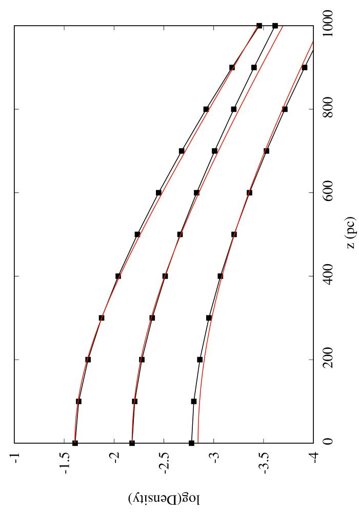
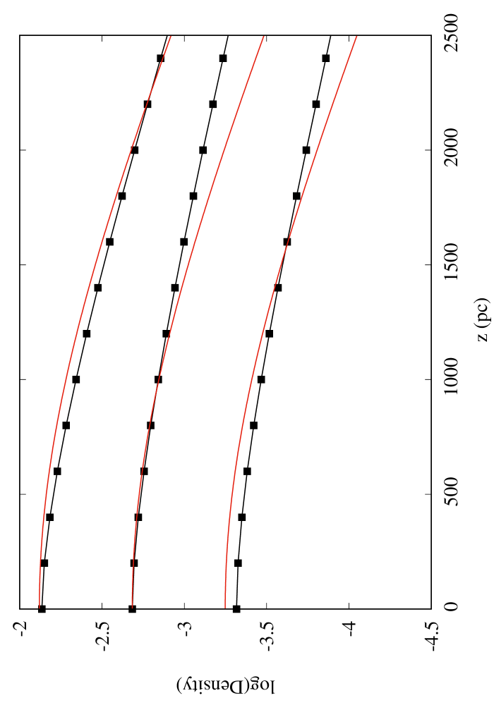
Figure 1: Vertical density distributions for the old thin stellar disc (left) and the old thick disc (right) at three Galactic radii $R$ = 4, 8, and 12 kpc. Red lines: the old thin disc Einasto profile (left) and the old thick disc profile (right) from the BGM2014 version. Black squares and lines: dynamically consistent fitted discs.

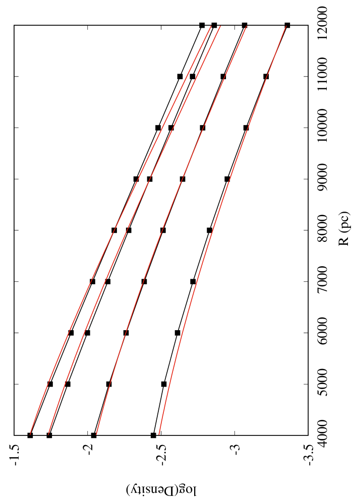
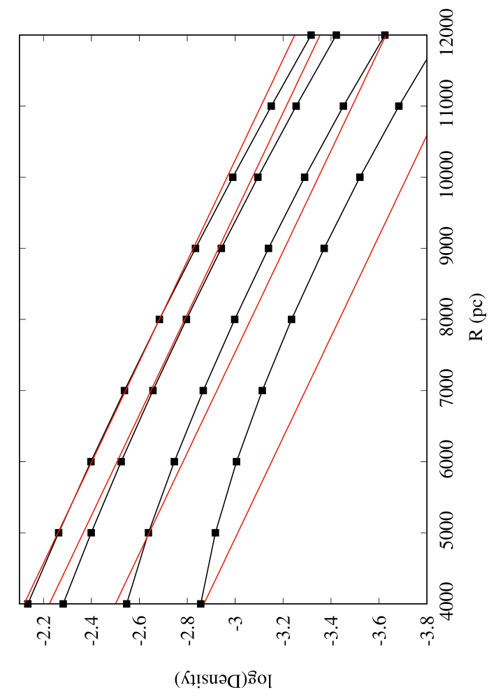
Figure 2: Radial density distributions for the old thin stellar disc (left) and the old thick disc (right) at four vertical heights $z$. Red lines: the old thin disc Einasto profile at $z$ = 0, 200, 400, and 600 pc (left) and the old thick disc profile at $z$ = 0, 0.8, 1.6, and 2.4 kpc (right) from the BGM2014 version. Black squares and lines: dynamically consistent disc fitted from $R$ = 4 kpc to 12 kpc.

Figure 1 (left) shows the vertical density distribution of the old thin disc (scale height around 230 pc) at three Galactic radii 4, 8, and 12 kpc, and Figure 2 (left) its radial distribution at four $z=$ 0, 200, 400, and 600 pc. The adjustment is satisfying. This is expected at $R$ = 8 kpc since the BGM2014 version is built to be dynamically consistent up to $z$ = 1 kpc. The fact that the fit is also satisfying at other galactic radii confirms that the choice of Einasto profiles in the BGM2014 version for the disc density was valuable with respect to the dynamics. For the other discs, the agreement between the BGM2014 and the new version is correct and is better for the thinner disc components with smaller vertical velocity dispersions. For the old thick disc, the vertical and radial density distributions (corresponding to a 795 pc scale height in the case of a $sech^{2}$ density law) are shown in Figures 1 and 2 (right). The agreement between both models is still correct. We note that at $R=8$ kpc and below $z$ = 1 kpc the fit is excellent, illustrating the exactness of the dynamical consistency of the BGM2014 version. However, at larger height above the Galactic plane, both models differ, and at two scale-heights, or 1.6 kpc height, the BGM2014 density for the old thick disc is 17 %  too small.

Concerning the density scale length, the agreement between the two models is nearly perfect for the old thin disc. For the old thick disc, the agreement is obtained only for $z$ lower than 1 kpc. We note that the flare present in the outskirts of the Galaxy could be naturally modelled by adjusting the vertical velocity dispersions at large Galactic radii.

Table 1 gives the relative difference in percentage between the new and the old models at different heights $z$ and at $R$ = 8 kpc, for the old thin and old thick discs. The differences increase with $z$; they become significant at three scale heights for the old thin disc and beyond 1 kpc for the old thick disc. At high $z$, the differences become of the order of the expected density of the stellar halo, and this illustrates the necessity of using dynamically self consistent distribution functions to properly identify and separate the Galactic stellar components. However, only observations will tell us whether our choice of nearly isothermal modelling of stellar discs is the correct one since small changes in the wings of the velocity distribution at low $z$ impact the vertical density distribution at high $z$. Other choices of DFs could produce similar densities and velocities at low $z$ and different densities at high $z$.

Table 1: Density differences (in percentage) between the BGM2004 version and the new dynamically self-consistent model for the old thin and old thick discs at $R$ = 8 kpc and various $z$.

old thin disc
z (pc)	200	400	600	800
diff(%)	-2.3%	-1.1%	+5%	+13%
old thick disc
z (pc)	800	1600	2400	3200
diff(%)	-2.5%	+17%	+60%	+263%

The vertical velocity dispersion of each stellar component at ($R_{\,0}$, $z$ = 0) is marginally modified in the new version compared with the BGM2014 version (see Table 2). This is a consequence of the fact that the self-consistency was already applied at low $z$.

Table 2: Previous (Robin et al. 2014, 2017) and new vertical velocity dispersions in km.s^-1 for disc 2 to 7 components and the two young and old thick disc components (8 and 9) at $R_{0}$= 8 kpc and $z$= 0.

disc	2	3	4	5	6	7	8	9
previous	8	10	13.2	15.8	17.4	17.5	28	59
new	7.3	9.9	13.4	16.0	17.5	17.6	26.4	51

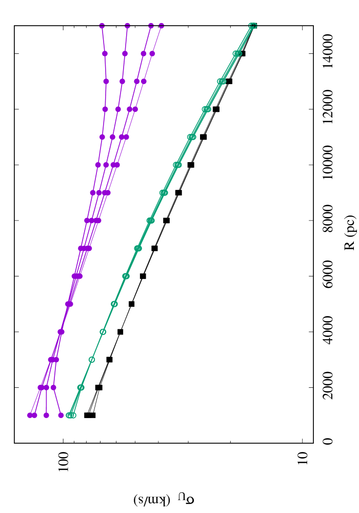
Figure 3: $\sigma_{U}$ radial velocity dispersions for the old thin disc (black lines) and the young thick disc (green lines) at $z$ = 0, 200, 400, and 600 pc. For the old thick disc (purple lines) at $z$ = 0, 0.8, 1.6, and 2.4 kpc. We note an increase in $\sigma_{U}$ and $R_{\sigma_{U}}$ with $z$ for the old thick disc.

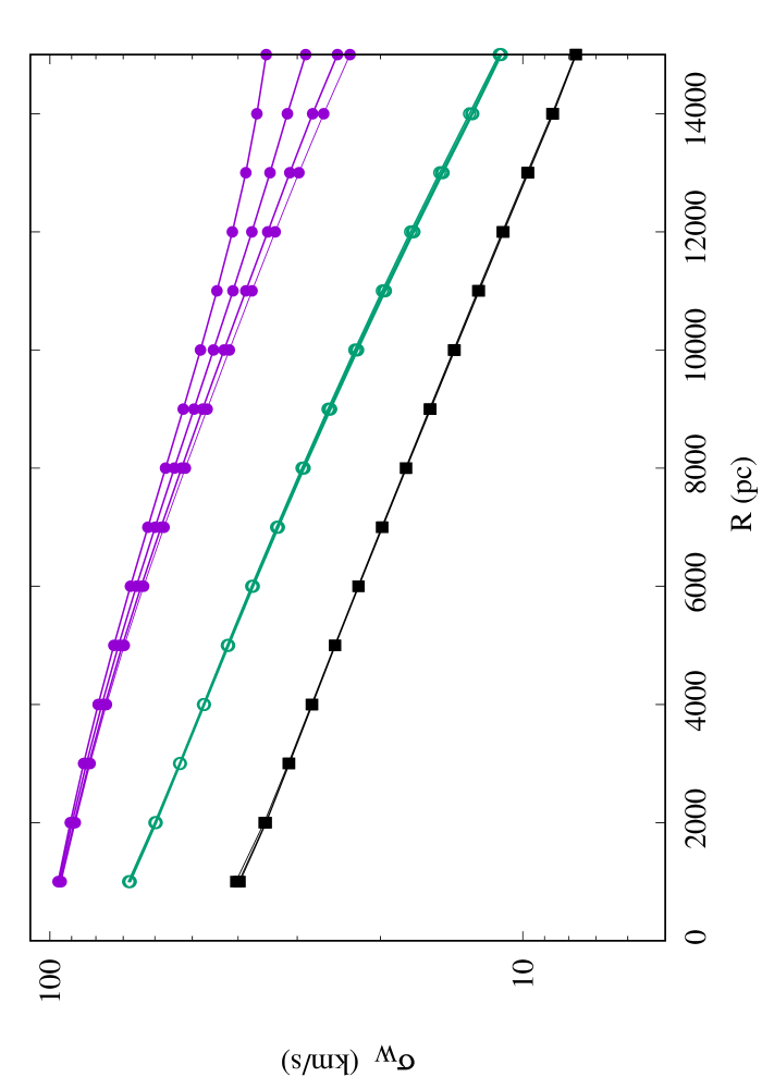
Figure 4: $\sigma_{W}$ vertical velocity dispersions for the old thin disc (black lines) and the young thick disc (green lines) at $z$ = 0, 200, 400, and 600 pc. For the old thick disc (purple lines) at $z$ = 0, 0.8, 1.6, and 2.4 kpc, $\sigma_{W}$ does not change with $z$ for the old thin disc or the young thick disc, but for the old thick disc, $\sigma_{W}$, and $R_{\sigma_{W}}$ increase with $z$.

Figure 3 shows at different $z$ the radial variations of $\sigma_{U}$ and Figure 4 the variations of $\sigma_{W}$. The velocity dispersions $\sigma_{U}$ and $\sigma_{W}$ are the major and minor axes of the velocity ellipsoid (i.e. $\sigma_{R}$ and $\sigma_{z}$ if $z=0$). By construction, their radial variations are nearly exponential. For the old thin disc, we do not see significant $z$-variation of the kinematical scale lengths, $R_{\sigma{{}_{R}}}$ and $R_{\sigma{{}_{z}}}$. For the old thick disc, the kinematic scale lengths increase with $z$. For the thin and thick discs discussed here, the respective density scale lengths $R_{\rho}$ at $z=0$ are 2.53 and 3.15 kpc, and the kinematic scale lengths $R_{\sigma_{z}}$ are 8.5 and 10.8 kpc. The ratio $R_{\sigma_{z}}/R_{\rho}$ is far from the factor 2, a frequently assumed value based on the hypothesis of a self-gravitating isothermal disc (van der Kruit & Searle 1981, 1982). At very small radii $R$, the asymmetric drift is very large for the old thick disc and moreover the DFs are null for negative angular momentum. Thus, the DFs are not realistic and it could explain the decrease in the dispersion at low $R$ and high $z$ (see Fig. 3).

The asymmetric drifts and the $\sigma_{V}$ velocity dispersions are no longer free parameters and are exactly determined. The asymmetric drifts (Figure 5) are shown as a function of $z$ at the solar Galactic radius $R_{0}$. The very different asymmetric drift of the old thick disc is due to its much higher velocity dispersions.

Within the interval $R=$ 4 to 12 kpc, the velocity ellipsoids roughly point towards the Galactic centre. Figure 6 shows the variation in the tilt with $z$ at $R$ = 8 kpc for all the stellar components. They are very similar and just the old thick disc has a tilt slightly larger by 1 degree at 4 kpc height. The velocity ellipsoid tilt variation for the stellar discs results from the different $z_{0}$ values defining the Stäckel coordinates to model the DFs. These different $z_{0}$ values are directly obtained by fitting the orbits populating the stellar discs. We can consider as a first approximation that the tilt does not depend on the stellar disc population.

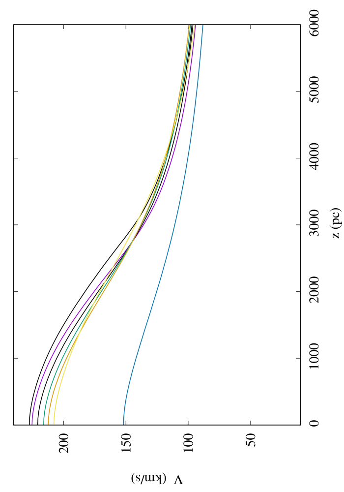
Figure 5: Mean circular velocities for all disc components vs. $z$ at $R$ = 8 kpc with $V_{c}(R_{\sun})$ = 221 km/s. The blue line corresponds to the old thick disc.

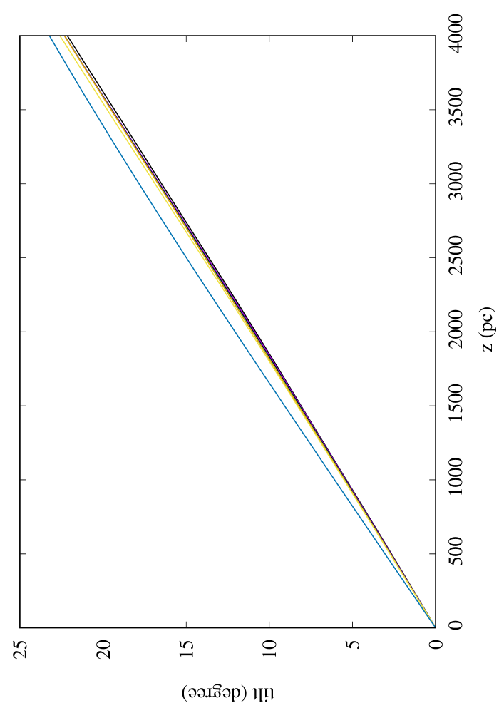
Figure 6: Velocity ellipsoid vertical tilts for stellar discs vs. $z$ at $R$ = 8 kpc. The blue line corresponds to the old thick disc.

6 Conclusion

We have presented the elements of the structure of the new dynamical self-consistency of the Besançon Galactic Model. It is based on the use of an explicit approximate third integral and on the 3D generalisation of the Shu DF. For each stellar disc, the number of free parameters is reduced since the vertical velocity dispersions and the scale heights are dynamically related for each stellar disc. In addition the density scale heights and the vertical kinematic scale lengths ($R_{\sigma_{z}})$ are linked. A preliminary and intermediate version of this model was used to adjust the stellar kinematics from RAVE and TGAS observations (Robin et al. 2017).

The consistency of the dynamical model is performed with an accuracy that allows us to recover the mass distribution and forces with an error smaller than a few thousandths. Since, this new model substantially reproduces the previous 2004 version of the Besançon model and its stellar densities, in consequence it also matches the star counts and then provides a prediction of the kinematics of stellar populations. These predictions will be compared with Gaia observations. We can expect that these new observations will entail revisions with an adjustment of the modelled stellar populations, and an improvement of our current representation of the dark matter distribution.

A precise determination of the mass distribution of the Galaxy and the dark matter component will only be only achieved with an accurate modelling of the observed stellar components and their kinematics. This is an immediate goal of the BGM. Furthermore, obtaining a stationary model of the stellar discs will be a preliminary step to estimate the degree of non-stationarity of stellar components. For each stellar population, the accuracy of the fit will give the amplitude of non-stationarities. This will help to identify what type of non-stationarities are involved and what kind of complementary models must be developed.

To conclude, we note that we have considered a stationary Galaxy model without a bar and our methods require axisymmetric potentials. Generalisation to a non-axisymmetric model (work in preparation) is however possible with the same simplicity since the method developed for axisymmetric potentials (Bienaymé et al. 2015) can be generalised to 3D, also with analytic approximate integrals explicitly depending on the potential without a need for numerical integrations (see also Sanders & Evans 2015; Sanders & Binney 2015).