Additive Schwarz Preconditioners for the Obstacle Problem of Clamped Kirchhoff Plates

Abstract.

When the obstacle problem of clamped Kirchhoff plates is discretized by a partition of unity method, the resulting discrete variational inequalities can be solved by a primal-dual active set algorithm. In this paper we develop and analyze additive Schwarz preconditioners for the systems that appear in each iteration of the primal-dual active set algorithm. Numerical results that corroborate the theoretical estimates are also presented.

1. Introduction

Let $\Omega$ be a bounded polygonal domain in $\mathbb{R}^{2}$, $f\in L_{2}(\Omega)$ and $\psi\in C(\bar{\Omega})\cap C^{2}(\Omega)$ such that $\psi<0$ on $\partial\Omega$. The obstacle problem for a clamped Kirchhoff plate occupying $\Omega$ is to find

(1.1) $$u=\mathop{\rm argmin}_{v\in K}\Big{[}\frac{1}{2}a(v,v)-(f,v)\big{]},$$

where $(\cdot,\cdot)$ is the inner product for $L_{2}(\Omega)$,

(1.2) $$a(v,w)=\int_{\Omega}D^{2}v:D^{2}w\,dx=\int_{\Omega}\sum_{i,j=1}^{2}\Big{(}\frac{\partial^{2}v}{\partial x_{i}\partial x_{j}}\Big{)}\Big{(}\frac{\partial^{2}w}{\partial x_{i}\partial x_{j}}\Big{)}dx\qquad\forall\,v,w\in H^{2}_{0}(\Omega),$$

and $K$ is the subset of $H^{2}_{0}(\Omega)$ defined by

(1.3) $$K=\{v\in H^{2}_{0}(\Omega):\,v\geq\psi\;\text{on}\;\Omega\}.$$

Here and throughout the paper we follow the standard notation for differential operators, function spaces and norms that can be found for example in [13, 1, 11].

Since $K$ is a nonempty closed convex subset of the Hilbert space $H^{2}_{0}(\Omega)$, it follows from the standard theory of calculus of variations [19, 24] that the obstacle problem (1.1) has a unique solution $u\in K$ characterized by the fourth order variational inequality

(1.4) $$a(u,v-u)-(f,v-u)\geq 0\qquad\forall\,v\in K.$$

The numerical solution of the obstacle problem (1.1)–(1.3) by a generalized finite element method was studied in [9]. The discrete variational inequalities resulting from the generalized finite element method were solved by a primal-dual active set algorithm [6, 7, 22, 23], where an auxiliary system of equations involving the inactive nodes had to be solved in each iteration. Since this is a fourth order problem, these systems become very ill-conditioned when the number of degrees of freedom becomes large. The goal of this paper is to develop one-level and two-level additive Schwarz domain decomposition preconditioners for the systems that appear in the primal-dual active set algorithm. We note that a two-level additive Schwarz preconditioner for the plate bending problem (without the obstacle) using the same generalized finite element method was investigated in [10].

There is a sizable literature on domain decomposition methods for second order variational inequalities [25, 38, 5, 33, 35, 36, 34, 4, 27, 12, 3, 26]. (References for related multigrid methods can be found in the survey article [20].) On the other hand the literature on domain decomposition methods for fourth order variational inequalities is quite small. The only work [31] that we know of treats an alternating Schwarz algorithm for the plate obstacle problem discretized by a mixed finite element method.

We note that most of the domain decomposition algorithms for variational inequalities are based on the subspace correction approach except the one in [26], where the author considered a multibody second order elliptic problem with inequality constraints on the interfaces of the bodies, and the nonoverlapping domain decomposition preconditioners in that paper are also designed for the auxiliary systems that appear in a primal-dual active set algorithm.

The rest of the paper is organized as follows. We recall the partition of unity method in Section 2 and the primal-dual active set algorithm in Section 3. We set up overlapping domain decomposition in Section 4 and study the one-level and two-level additive Schwarz preconditioners in Section 5 and Section 6. Numerical results that corroborate the theoretical estimates are presented in Section 7 and we end with some concluding remarks in Section 8.

2. A Partition of Unity Method

Conforming finite element methods for the fourth order problem (1.1)–(1.3) require $C^{1}$ finite element spaces. In the classical setting this would involve polynomials of high degrees in the construction of the local approximation spaces [13, 11]. An alternative is to employ generalized finite element methods [28, 2]. This was carried out in [9] using a flat-top partition of unity method (PUM) from [21, 30, 29, 14]. Below we recall some basic facts concerning the PUM in [9].

Let $\{\Omega_{i}\}_{i=1}^{n}$ be an open cover of $\bar{\Omega}$ such that there exists a collection of nonnegative functions $\phi_{1},\ldots,\phi_{n}\in W^{2}_{\infty}(\mathbb{R}^{2})$ with the following properties:

$$\text{supp}\,\phi_{i} \subset\Omega_{i} \text{for}\;1\leq i\leq n,$$

$$\sum_{i=1}^{n}\phi_{i} =1 \text{on}\;\Omega,$$

$$|\phi_{i}|_{W^{m}_{\infty}(\mathbb{R}^{2})} \leq\frac{C}{(\text{diam}\,\Omega_{i})^{m}} \text{for}\;0\leq m\leq 2,\;1\leq i\leq n.$$

From here on we use $C$ (with or without subscript) to denote a generic positive constant that can take different values at different appearances.

Let $V_{i}$ be a subspace of biquadratic polynomials defined on the local patch $\Omega_{i}$ whose members satisfy the homogeneous Dirichlet boundary conditions on $\partial\Omega$. The generalized finite element space $V_{G}\subset H^{2}_{0}(\Omega)$ is given by

$$V_{G}=\sum_{i=1}^{n}\phi_{i}V_{i}.$$

There are many choices in the construction of the partition of unity. We use a flat-top partition of unity where each $\Omega_{i}$ is an open rectangle and each $\phi_{i}$ is the tensor product of two one dimensional flat-top functions. The flat-top region $\Omega_{i}^{\rm flat}$ inside $\Omega_{i}$ is the set where $\phi_{i}=1$, and the degrees of freedom for the local space $V_{i}$ are all associated with nodes on $\Omega_{i}^{\rm flat}$. An illustration for such a construction is given in Figure 2.1 for a square domain $\Omega$. Details for the construction and examples for other domains can be found in [9].

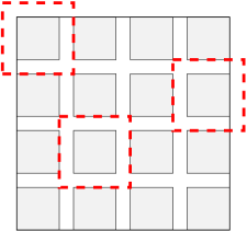
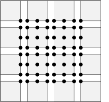
Figure 2.1. (a) $\Omega_{i}$ (bounded by dotted lines) and $\Omega_{i}^{\rm flat}$ (shaded in grey) (b) nodes for the interior DOFs

From now on we assume that the diameters of the patches are comparable to a mesh size $h$ and denote the generalized finite element space by $V_{h}$. Let $\mathcal{N}_{h}$ be the set of the nodes in the local patches (solid dots in Figure 2.1 (b)) that correspond to the degrees of freedom of the local basis functions. (The cardinality of $\mathcal{N}_{h}$ is the dimension of $V_{h}$.) The discrete problem is to find

(2.1) $$u_{h}=\mathop{\rm argmin}_{v\in K_{h}}\Big{[}\frac{1}{2}a(v,v)-(f,v)\Big{]},$$

where

(2.2) $$K_{h}=\{v\in V_{h}:\,v(p)\geq\psi(p)\quad\forall\,p\in\mathcal{N}_{h}\}.$$

Remark 2.1.

Since the nodes in $\mathcal{N}_{h}$ are located at the flat-top regions of the local patches, the constraints for $K_{h}$ are box constraints.

Let the interpolation operator $\Pi_{h}:H^{2}_{0}(\Omega)\longrightarrow V_{h}$ be defined by

(2.3) $$\Pi_{h}\zeta=\sum_{i=1}^{n}(\Pi_{i}\zeta)\phi_{i},$$

where $\Pi_{i}$ is the local nodal interpolation operator for $V_{i}$. Then $\Pi_{h}u$ belongs to $K_{h}$ and hence $K_{h}$ is a nonempty closed convex subset of $V_{h}$. It follows from the standard theory that (2.1) has a unique solution $u_{h}\in K_{h}$ characterized by the discrete variational inequality

(2.4) $$a(u_{h},v-u_{h})-(f,v-u_{h})\geq 0\qquad\forall\,v\in K_{h}.$$

Moreover we have [9, Theorem 3.2]

$$|u-u_{h}|_{H^{2}(\Omega)}\leq Ch^{\alpha},$$

where the index of elliptic regularity $\alpha\in(\frac{1}{2},1]$ is determined by the angles at the corners of $\Omega$ and we can take $\alpha$ to be $1$ if $\Omega$ is convex.

We will need the following interpolation error estimate [9, (2.9)] in the analysis of the domain decomposition preconditioners:

(2.5) $$\sum_{m=0}^{1}h^{m}|\zeta-\Pi_{h}\zeta|_{H^{m}(\Omega)}+h^{2}|\Pi_{h}\zeta|_{H^{2}(\Omega)}\leq C_{\Pi}h^{2}|\zeta|_{H^{2}(\Omega)}\qquad\forall\,\zeta\in H^{2}(\Omega),$$

where the positive constant $C_{\Pi}$ is independent of $h$.

We will also need the trivial estimate

(2.6) $$\|v\|_{L_{2}(\Omega)}\approx\sum_{p\in\mathcal{N}_{h}}v^{2}(p)\qquad\forall\,v\in V_{h}$$

that follows from standard estimates for the biquadratic polynomials defined over the patches.

3. A Primal-Dual Active Set Algorithm

Let the function $\lambda_{h}:\mathcal{N}_{h}\longrightarrow\mathbb{R}$ be defined by

(3.1) $$a(u_{h},v)-(f,v)=\sum_{p\in\mathcal{N}_{h}}\lambda_{h}(p)v(p)\qquad\forall\,v\in V_{h}.$$

The discrete variational inequality (2.4) is equivalent to (3.1) together with the optimality conditions

$$u_{h}(p)-\psi(p)\geq 0,\quad\lambda_{h}(p)\geq 0\quad\text{and}\quad(u_{h}(p)-\psi(p))\lambda_{h}(p)=0\qquad\forall\,p\in\mathcal{N}_{h},$$

which can also be written concisely as

(3.2) $$\lambda_{h}(p)=\max\big{(}0,\lambda_{h}(p)+c(\psi(p)-u_{h}(p))\big{)}\qquad\forall\,p\in\mathcal{N}_{h}.$$

Here $c$ can be any positive number.

The system defined by (3.1) and (3.2) can be solved by a semi-smooth Newton iteration that is equivalent to a primal-dual active set method [6, 7, 22, 23]. Given an approximation $(u_{k},\lambda_{k})$ of $(u_{h},\lambda_{h})$, the semi-smooth Newton iteration obtains the next approximation by solving the following system of equations:

(3.3a) $$a(u_{k+1},v)-(f,v) =\sum_{p\in\mathcal{N}_{h}}\lambda_{k+1}(p)v(p) \forall\,v\in V_{h},$$

(3.3b) $$u_{k+1}(p) =\psi(p) \forall\,p\in\mathfrak{A}_{k},$$

(3.3c) $$\lambda_{k+1}(p) =0 \forall\,p\in\mathcal{N}_{h}\setminus\mathfrak{A}_{k},$$

where $\mathfrak{A}_{k}=\{p\in\mathcal{N}_{h}:\lambda_{k}(p)+c(\psi(p)-u_{k}(p))>0\}$ is the active set determined by $(u_{k},\lambda_{k})$ and $c$ is a (large) positive constant. The iteration terminates when $\mathfrak{A}_{k+1}=\mathfrak{A}_{k}$.

In view of (3.3b) and (3.3c), we can reduce (3.3a) to an auxiliary system that only involves the unknowns $u_{k+1}(p)$ for $p\in\mathcal{N}_{h}\setminus\mathfrak{A}_{k}$. For small $h$, this is a large, sparse and ill-conditioned system that can be solved efficiently by a preconditioned Krylov subspace method, such as the preconditioned conjugate gradient method.

This preconditioning problem can be posed in the following general form. Let $\widetilde{\mathcal{N}}_{h}$ be a subset of $\mathcal{N}_{h}$. We define the truncation operator $\tilde{T}_{h}:V_{h}\longrightarrow V_{h}$ by

(3.4) $$(\tilde{T}_{h}v)(p)=\begin{cases}v(p)&\qquad\text{if $p\in\widetilde{\mathcal{N}}_{h}$}\\[4.0pt] 0&\qquad\text{if $p\in\mathcal{N}_{h}\setminus\widetilde{\mathcal{N}}_{h}$}\end{cases}.$$

Then $\tilde{T}_{h}$ is a projection from $V_{h}$ onto $\widetilde{V}_{h}=\tilde{T}_{h}V_{h}$.

Let $\tilde{A}_{h}:\widetilde{V}_{h}\longrightarrow\widetilde{V}_{h}^{\prime}$ be defined by

(3.5) $$\langle\tilde{A}_{h}v,w\rangle=a(v,w)\qquad\forall\,v,w\in\widetilde{V}_{h},$$

where $\langle\cdot,\cdot\rangle$ is the canonical bilinear form on $V_{h}^{\prime}\times V_{h}$. We want to construct preconditioners for $\tilde{A}_{h}$ whose performance is independent of $\widetilde{\mathcal{N}}_{h}$. Since the partition of unity method is defined in terms of overlapping patches, it is natural to consider additive Schwarz domain decomposition preconditioners [18].

Note that (2.6) implies

(3.6) $$\|\tilde{T}_{h}v\|_{L_{2}(\Omega)}\leq C\|v\|_{L_{2}(\Omega)}\qquad\forall\,v\in V_{h}.$$

4. Domain Decomposition

Let the subdomains $\{D_{j}\}_{j=1}^{J}$ form an overlapping domain decomposition of $\Omega$ such that

(4.1) $$\text{diam}\,D_{j}\approx H\qquad\text{for}\;1\leq j\leq J,$$

and

(4.2) $$\text{any point in $\Omega$ can belong to at most $N_{c}$ many subdomains}.$$

We also assume that the boundaries of $D_{1},\ldots,D_{J}$ are aligned with the boundaries of the patches underlying the generalized finite element space $V_{h}$. An example of four overlapping subdomains for a square domain $\Omega$ is depicted in Figure 4.1. Details for the construction of $D_{1},\ldots,D_{J}$ are available in [10].

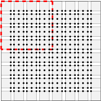
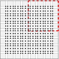
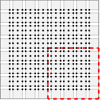
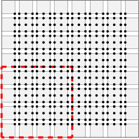
Figure 4.1. Domain decomposition for a square domain $\Omega$ with four overlapping subdomains (bounded by the dotted lines)

Note that (4.1) implies

(4.3) $$J\approx H^{-2},$$

provided that the subdomains $D_{1},\ldots,D_{J}$ are shape regular.

We assume that there exists a partition of unity $\psi_{1},\ldots,\psi_{J}\in W^{2}_{\infty}(\mathbb{R}^{2})$ with the following properties:

(4.4a) $$\sum_{j=1}^{J}\psi_{j} =1 \text{on}\;\bar{\Omega},$$

(4.4b) $$\psi_{j} \geq 0 \text{for }j=1,\ldots J,$$

(4.4c) $$\psi_{j} =0 \text{on }\Omega\setminus\bar{D}_{j},\;1\leq j\leq J,$$

(4.4d) $$|\psi_{j}|_{W^{k}_{\infty}(\Omega)} \leq C_{\dagger}\delta^{-k} \text{for }j=1,\ldots,J\text{ and }k=0,1,2.$$

Here $\delta$ $(\geq h)$ measures the overlap among the subdomains $D_{1},\ldots,D_{J}$.

5. A One-Level Additive Schwarz Preconditioner

Let $\widetilde{V}_{j}$ be the subspace of $\widetilde{V}_{h}$ whose members vanish at all the nodes outside $D_{j}$ and $A_{j}:\widetilde{V}_{j}\longrightarrow\widetilde{V}_{j}^{\prime}$ be defined by

(5.1) $$\langle A_{j}v,w\rangle=a(v,w)\qquad\forall\,v,w\in\widetilde{V}_{j}.$$

The one-level additive Schwarz preconditioner $B_{\scriptscriptstyle\rm OL}:\widetilde{V}_{h}^{\prime}\longrightarrow\widetilde{V}_{h}$ is defined by

(5.2) $$B_{\scriptscriptstyle\rm OL}=\sum_{j=1}^{J}I_{j}A_{j}^{-1}I_{j}^{t},$$

where $I_{j}:\widetilde{V}_{j}\longrightarrow\widetilde{V}_{h}$ is the natural injection.

Theorem 5.1.

We have

(5.3) $$\kappa(B_{\scriptscriptstyle\rm OL}\tilde{A}_{h})=\frac{\lambda_{\max}(B_{\scriptscriptstyle\rm OL}\tilde{A}_{h})}{\lambda_{\min}(B_{\scriptscriptstyle\rm OL}\tilde{A}_{h})}\leq C\delta^{-4},$$

where $\delta$ $(\geq h)$ measures the overlap among the subdomains $D_{1},\ldots,D_{J}$ and the positive constant $C$ is independent of $h$, $H$, $J$, $\delta$ and $\widetilde{\mathcal{N}}_{h}$.

Proof.

Let $v_{j}\in\widetilde{V}_{j}$, $1\leq j\leq J$, be arbitrary. We have a standard estimate [10, Lemma 1]:

(5.4) $$a\Big{(}\sum_{j=1}^{J}I_{j}v_{j},\sum_{j=1}^{J}I_{j}v_{j}\Big{)}\leq C_{\sharp}\sum_{j=1}^{J}a(v_{j},v_{j}),$$

where the positive constant $C_{\sharp}$ only depends on $N_{c}$. It follows from the standard additive Schwarz theory [32, 37, 27, 11] that

(5.5) $$\lambda_{\max}(B_{\scriptscriptstyle\rm OL}\tilde{A}_{h})\leq C_{\sharp}.$$

Given any $v\in\widetilde{V}_{h}$, we have $v_{j}=\Pi_{h}(\psi_{j}v)\in\widetilde{V}_{j}$,

(5.6) $$\sum_{j=1}^{J}v_{j}=\Pi_{h}\Big{[}\Big{(}\sum_{j=1}^{J}\psi_{j}\Big{)}v\Big{]}=\Pi_{h}v=v,$$

and

$$\sum_{j=1}^{J}a(v_{j},v_{j}) =\sum_{j=1}^{J}a\big{(}\Pi_{h}(\psi_{j}v),\Pi_{h}(\psi_{j}v)\big{)}$$

$$=\sum_{j=1}^{J}|\Pi_{h}(\psi_{j}v)|_{H^{2}(\Omega)}^{2}$$

$$\leq C\sum_{j=1}^{J}|\psi_{j}v|_{H^{2}(\Omega)}^{2}$$

(5.7) $$\leq C\sum_{j=1}^{J}\sum_{k=0}^{2}|\psi_{j}|^{2}_{W^{2-k}_{\infty}(\Omega)}|v|_{H^{k}(D_{j})}^{2}$$

$$\leq C\sum_{k=0}^{2}\delta^{-2(2-k)}\sum_{j=1}^{J}|v|_{H^{k}(D_{j})}^{2}$$

$$\leq C\sum_{k=0}^{2}\delta^{-2(2-k)}|v|_{H^{k}(\Omega)}^{2}$$

$$\leq C_{\flat}\delta^{-4}|v|_{H^{2}(\Omega)}^{2}$$

$$=C_{\flat}\delta^{-4}a(v,v),$$

where the positive constant $C_{\flat}$ depends only on $C_{\Pi}$ in (2.5), $N_{c}$ in (4.2), $C_{\dagger}$ in (4.4d) and constants for Poincaré-Friedrichs inequalities associated with $H^{2}_{0}(\Omega)$.

It follows from (5.6), (5) and the standard additive Schwarz theory that

(5.8) $$\lambda_{\min}(B_{\scriptscriptstyle\rm OL}\tilde{A}_{h})\geq\delta^{4}C_{\flat}^{-1}.$$

The estimates (5.5) and (5.8) imply (5.3) with $C=C_{\sharp}C_{\flat}$. ∎

Remark 5.2.

The estimate (5.3) is identical to the one for the plate bending problem without an obstacle, i.e., the obstacle is invisible to the one-level additive Schwarz preconditioner.

Remark 5.3.

Under the assumption that the subdomains $D_{1},\ldots,D_{J}$ are shape regular, we can improve the estimate (5.3) to

(5.9) $$\kappa(B_{\scriptscriptstyle\rm OL}\tilde{A}_{h})\leq C\delta^{-3}H^{-1}$$

by the arguments in [8, Section 8]. (Similar arguments for second order problems can be found in [37, Lemma 3.10].) We will assume this is the case in the discussion below.

Since $\delta$ decreases as $H$ decreases (or equivalently as $J$ increases), the one-level algorithm is not a scalable algorithm. Nevertheless the condition number estimate (5.9) can still be a big improvement over the estimate $\kappa(\tilde{A}_{h})\approx h^{-4}$ for the original system.

5.1. Small Overlap

In the case of small overlap among the subdomains, we have $\delta\approx h$, and hence

(5.10) $$\kappa(B_{\scriptscriptstyle\rm OL}\tilde{A}_{h})\leq Ch^{-3}H^{-1},$$

which indicates that asymptotically

(5.11) $$\kappa(B_{\scriptscriptstyle\rm OL}\tilde{A}_{h}) 8 H$$ will increase by a factor of after each refinement if is kept fixed.

On the other hand the estimate (5.10) also indicates that

(5.12) $$\kappa(B_{\scriptscriptstyle\rm OL}\tilde{A}_{h}) 2 H$$ will increase by a factor of if decreases by a factor of 2

(or equivalently if $$J 4 h$$ increases by a factor of ) while is kept fixed.

5.2. Generous Overlap

In the case of generous overlap among the subdomains, we have $\delta\approx H$, and hence

(5.13) $$\kappa(B_{\scriptscriptstyle\rm OL}\tilde{A}_{h})\leq CH^{-4}\approx J^{2}.$$

It follows from (5.13) that

(5.14) $$\kappa(B_{\scriptscriptstyle\rm OL}\tilde{A}_{h}) J$$ increases as increases,

and

(5.15) $$\kappa(B_{\scriptscriptstyle\rm OL}\tilde{A}_{h}) h H J$$ remains constant as decreases provided (equivalently )

is kept fixed.

6. A Two-Level Additive Schwarz Preconditioner

Let $V_{H}$ be a coarse generalized finite element subspace of $H^{2}_{0}(\Omega)$ associated with patches whose diameters are comparable to the diameters of the subdomains $D_{1},\ldots,D_{J}$ in the decomposition of $\Omega$. We define $\widetilde{V}_{0}\subset\widetilde{V}_{h}$ by

(6.1) $$\widetilde{V}_{0}=\tilde{T}_{h}\Pi_{h}V_{H},$$

and the operator $A_{0}:\widetilde{V}_{0}\longrightarrow\widetilde{V}_{0}^{\prime}$ by

(6.2) $$\langle A_{0}v,w\rangle=a(v,w)\qquad\forall\,v,w\in\widetilde{V}_{0}.$$

The two-level additive Schwarz preconditioner $B_{\scriptscriptstyle\rm TL}:\widetilde{V}_{h}^{\prime}\longrightarrow\widetilde{V}_{h}$ is given by

(6.3) $$B_{\scriptscriptstyle\rm TL}=\sum_{j=0}^{J}I_{j}A_{j}^{-1}I_{j}^{t},$$

where $I_{0}:\widetilde{V}_{0}\longrightarrow\widetilde{V}_{h}$ is also the natural injection.

Let $Q_{H}$ be the orthogonal projection from $L_{2}(\Omega)$ onto $V_{H}$. The operator $R_{0}:V_{h}\longrightarrow\widetilde{V}_{0}$ is defined by

(6.4) $$R_{0}v=\tilde{T}_{h}\Pi_{h}Q_{H}v\qquad\forall\,v\in V_{h}.$$

The following result is useful for the analysis of $B_{\scriptscriptstyle\rm TL}$.

Lemma 6.1.

We have

(6.5) $$\|v-R_{0}v\|_{L_{2}(\Omega)}+h|v-R_{0}v|_{H^{1}(\Omega)}+h^{2}|v-R_{0}v|_{H^{2}(\Omega)}\leq CH^{2}|v|_{H^{2}(\Omega)}\qquad\forall\,v\in\widetilde{V}_{h}.$$

Proof.

From (2.5) we have the estimate

$$\|\zeta-Q_{H}\zeta\|_{L_{2}(\Omega)}\leq CH^{2}|\zeta|_{H^{2}(\Omega)}\qquad\forall\,\zeta\in H^{2}(\Omega),$$

which together with (2.5) and (3.6) implies that, for any $v\in\widetilde{V}_{h}$,

$$\|v-R_{0}v\|_{L_{2}(\Omega)} =\|v-\tilde{T}_{h}\Pi_{h}Q_{H}v\|_{L_{2}(\Omega)}$$

$$\leq\|\tilde{T}_{h}(v-\Pi_{h}Q_{H}v)\|_{L_{2}(\Omega)}$$

$$\leq C\|v-\Pi_{h}Q_{H}v\|_{L_{2}(\Omega)}$$

$$\leq C\big{(}\|v-\Pi_{h}v\|_{L_{2}(\Omega)}+\|\Pi_{h}(v-Q_{H}v)\|_{L_{2}(\Omega)}\big{)}$$

$$\leq C\big{(}\|v-\Pi_{h}v\|_{L_{2}(\Omega)}+\|v-Q_{H}v\|_{L_{2}(\Omega)}\big{)}$$

$$\leq CH^{2}|v|_{H^{2}(\Omega)}.$$

The estimates for $|v-R_{0}v|_{H^{1}(\Omega)}$ and $|v-R_{0}v|_{H^{2}(\Omega)}$ then follow from inverse estimates. ∎

Theorem 6.2.

We have

(6.6) $$\kappa(B_{\scriptscriptstyle\rm TL}\tilde{A}_{h})=\frac{\lambda_{\max}(B_{\scriptscriptstyle\rm TL}\tilde{A}_{h})}{\lambda_{\min}(B_{\scriptscriptstyle\rm TL}\tilde{A}_{h})}\leq C\min\big{(}(H/h)^{4},\delta^{-4}\big{)},$$

where the positive constant $C$ is independent of $H$, $h$, $J$, $\delta$ and $\widetilde{\mathcal{N}}_{h}$.

Proof.

The following upper bound for the maximum eigenvalue of $B_{\scriptscriptstyle\rm TL}\tilde{A}_{h}$ is again standard [10, Lemma 1]:

(6.7) $$\lambda_{\max}(B_{\scriptscriptstyle\rm TL}\tilde{A}_{h})\leq\tilde{C}_{\sharp},$$

where $\tilde{C}_{\sharp}$ only depends on the number $N_{c}$ in (4.2).

Let $v\in\widetilde{V}_{h}$ be arbitrary, $v_{0}=R_{0}v\in\widetilde{V}_{0}$ and $v_{j}=\Pi_{h}(\psi_{j}(v-v_{0}))\in\widetilde{V}_{j}$. We have

(6.8) $$\sum_{j=0}^{J}v_{j}=v_{0}+\Pi_{h}\Big{[}\Big{(}\sum_{j=1}^{J}\psi_{j}\Big{)}(v-v_{0})\Big{]}=v_{0}+(v-v_{0})=v,$$

and, by (6.5),

(6.9) $$a(v_{0},v_{0})=|R_{0}v|_{H^{2}(\Omega)}^{2} \leq 2|v-R_{0}v|_{H^{2}(\Omega)}^{2}+2|v|_{H^{2}(\Omega)}^{2}$$

$$\leq C(1+H^{4}h^{-4})|v|_{H^{2}(\Omega)}^{2}\leq CH^{4}h^{-4}a(v,v).$$

Using (4.4d) and (6.5) we also find

$$\sum_{j=1}^{J}a(v_{j},v_{j}) =\sum_{j=1}^{J}|\Pi_{h}(\psi_{j}(v-v_{0}))|_{H^{2}(\Omega)}^{2}$$

$$\leq C\sum_{j=1}^{J}|\psi_{j}(v-v_{0})|_{H^{2}(\Omega)}^{2}$$

$$\leq C\sum_{j=1}^{J}\sum_{k=0}^{2}|\psi_{j}|_{W^{2-k}_{\infty}(\Omega)}^{2}|v-R_{0}v|_{H^{k}(D_{j})}^{2}$$

(6.10) $$\leq C\sum_{k=0}^{2}\delta^{-2(2-k)}\sum_{j=1}^{J}|v-R_{0}v|_{H^{k}(D_{j})}^{2}$$

$$\leq C\sum_{k=0}^{2}\delta^{-2(2-k)}|v-R_{0}v|_{H^{k}(\Omega)}^{2}$$

$$\leq C\Big{(}\frac{H^{4}}{\delta^{4}}+\frac{H^{4}}{\delta^{2}h^{2}}+\frac{H^{4}}{h^{4}}\Big{)}|v|_{H^{2}(\Omega)}^{2}$$

$$\leq C(H/h)^{4}a(v,v).$$

It follows from (6.8)–(6) that

$$\sum_{j=0}^{J}a(v_{j},v_{j})\leq\tilde{C}_{\flat}(H/h)^{4}a(v,v).$$

On the other hand, by taking $v_{0}=0$ and $v_{j}=\Pi_{h}(\psi_{j}v)$ for $1\leq j\leq J$, we have

$$\sum_{j=0}^{J}a(v_{j},v_{j})\leq C_{\flat}\delta^{-4}a(v,v)$$

by (5). Hence the standard theory for additive Schwarz preconditioners implies that

(6.11) $$\lambda_{\min}(B_{\scriptscriptstyle\rm TL}\tilde{A}_{h})\geq\frac{1}{\min\big{(}\tilde{C}_{\flat}(H/h)^{4},C_{\flat}\delta^{-4}\big{)}}.$$

Consequently the estimate (6.6) holds with $C=\tilde{C}_{\sharp}\max(\tilde{C}_{\flat},C_{\flat})$. ∎

Remark 6.3.

The estimate (6.6) is different from the estimate for the plate bending problem without obstacles that reads

$$\kappa(B_{\scriptscriptstyle\rm TL}A_{h})\leq C\Big{(}\frac{H}{\delta}\Big{)}^{4}.$$

This difference is caused by the necessity of truncation in the construction of $\widetilde{V}_{0}$ when the obstacle is present.

Remark 6.4.

Under the assumption that the subdomains $D_{1},\ldots,D_{J}$ are shape regular, the estimate (6.6) can be improved to

(6.12) $$\kappa(B_{\scriptscriptstyle\rm TL}\tilde{A}_{h})\leq C\min\big{(}(H/h)^{4},\delta^{-3}H^{-1}\big{)}.$$

We will assume this is the case in the discussion below.

The estimates (6.12) indicate that the two-level algorithm is scalable as long as the ratio $H/h$ remains bounded, and

(6.13) the condition number for the two-level algorithm is (up to a constant) at least

as good as the one-level algorithm.

6.1. Small Overlap

In the case of small overlap where $\delta\approx h$, we have

$$(H/h)^{4}\ll h^{-3}H^{-1}\quad\text{if $H^{5}\ll h$},$$

which indicates that

(6.14) $$\kappa(B_{\scriptscriptstyle\rm TL}\tilde{A}_{h})<\kappa(B_{\scriptscriptstyle\rm OL}\tilde{A}_{h})\quad\text{for small $H$ (or equivalently for large $J$) if $h$ is kept fixed.}$$

6.2. Generous Overlap

In the case of generous overlap where $\delta\approx H$, we have the following analog of (5.15):

(6.15) $$\kappa(B_{\scriptscriptstyle\rm TL}\tilde{A}_{h}) h H J$$ remains constant as decreases provided (equivalently )

is kept fixed.

Moreover, we have

$$(H/h)^{4}\ll H^{-4}\quad\text{if $H^{2}\ll h$},$$

which again indicates that

(6.16) $$\kappa(B_{\scriptscriptstyle\rm TL}\tilde{A}_{h})<\kappa(B_{\scriptscriptstyle\rm OL}\tilde{A}_{h})\quad\text{for small $H$ (or equivalently for large $J$) if $h$ is kept fixed.}$$

7. Numerical Results

We consider the obstacle problem in [9, Example 4.2], where $\Omega=(-0.5,0.5)^{2}$, $f=0$ and $\psi(x)=1-5|x|^{2}+|x|^{4}$. We discretize (1.1) by the PUM using rectangular patches (cf. Figure 2.1) with $h\approx 2^{-\ell}$, where $\ell$ is the refinement level. As $\ell$ increases from 1 to 8, the number of degrees of freedom increases from 4 to 583696. The discrete variational inequalities are solved by the primal-dual active set (PDAS) algorithm in Section 3.

For the purpose of comparison, we first solve the auxiliary systems in each iteration of the PDAS algorithm by the conjugate gradient (CG) method without a preconditioner. The average condition number during the PDAS iteration and the time to solve the variational inequality are presented in Table 7.1. The PDAS iterations fail to stop (DNC) within 48 hours at level $8$.

Table 7.1. Average condition number ($\kappa$) and time to solve the variational inequality ($t_{\text{solve}}$) by the CG algorithm

$\ell$	$\kappa$	$t_{\text{solve}}$ (sec)
1	$1.0000\times 10^{0}$	$8.4889\times 10^{-2}$
2	$2.8251\times 10^{2}$	$1.1865\times 10^{-1}$
3	$6.2071\times 10^{3}$	$8.7772\times 10^{-1}$
4	$9.3827\times 10^{4}$	$9.7040\times 10^{+0}$
5	$1.7843\times 10^{6}$	$1.1611\times 10^{+2}$
6	$3.0294\times 10^{7}$	$4.3516\times 10^{+3}$
7	$4.9776\times 10^{8}$	$9.8090\times 10^{+4}$
8	$8.0687\times 10^{9}$	DNC

We then solve the auxiliary systems by the preconditioned conjugate gradient (PCG) method, using the additive Schwarz preconditioners associated with $J$ subdomains. The mesh size $H$ for the coarse generalized finite element space is $\approx 1/\sqrt{J}$. We say the PCG method has converged if $\|Br\|_{2}\leq 10^{-15}\|b\|_{2},$ where $B$ is the preconditioner, $r$ is the residual, and $b$ is the load vector. The initial guess for the PDAS algorithm is taken to be the solution at the previous level, or 0 if $2^{2\ell}=J$. The subdomain problems and coarse problem are solved by a direct method based on the Cholesky factorization.

7.1. Small Overlap

In this case we have $\delta\approx h$. The numbers of PDAS iterations for the one-level and two-level algorithms are given in Table 7.2. The results are similar. (The numbers only differ at three locations where they appear in red.) For both algorithms, the PDAS iterations fail to stop within 48 hours at level $8$ when $J=4$, which is due to the large sizes of the subdomain problems.

Table 7.2. Number of PDAS iterations with small overlap

	$J=4$		$J=16$		$J=64$		$J=256$
$\ell$	one-level	two-level	one-level	two-level	one-level	two-level	one-level	two-level
1	1	1	-	-	-	-	-	-
2	5	5	4	4	-	-	-	-
3	12	12	12	12	14	14	-	-
4	21	21	21	21	21	30	29	29
5	22	22	22	22	22	22	22	47
6	47	47	47	47	47	47	47	89
7	66	66	66	66	66	66	66	66
8	DNC	DNC	64	64	64	64	64	64

The average condition number of the preconditioned auxiliary systems during the PDAS iterations are reported in Tables 7.3 and 7.4. Comparing to the average condition number in Table 7.1, both algorithms show marked improvement. The behavior of the condition numbers for the one-level algorithm in Table 7.3 agrees with the observations in (5.11) and (5.12). A comparison of Table 7.3 and Table 7.4 shows that

$$\max\frac{\kappa(B_{\scriptscriptstyle\rm TL}\tilde{A}_{h})}{\kappa(B_{\scriptscriptstyle\rm OL}\tilde{A}_{h})}\approx 1.24,$$

where the maximum is taken over all the corresponding entries in Table 7.3 and Table 7.4, which agrees with (6.13). Moreover, $\kappa(B_{\scriptscriptstyle\rm TL}\tilde{A}_{h})$ is smaller than $\kappa(B_{\scriptscriptstyle\rm OL}\tilde{A}_{h})$ for $J$ large, as observed in (6.14).

Table 7.3. Average condition number, one-level with small overlap

$\ell$	$J=4$	$J=16$	$J=64$	$J=256$
1	$0.000\times 10^{+0}$	-	-	-
2	$3.950\times 10^{+0}$	$2.187\times 10^{+0}$	-	-
3	$4.351\times 10^{+0}$	$6.395\times 10^{+0}$	$5.886\times 10^{+0}$	-
4	$4.928\times 10^{+0}$	$1.116\times 10^{+1}$	$2.301\times 10^{+1}$	$3.751\times 10^{+1}$
5	$9.825\times 10^{+0}$	$6.154\times 10^{+1}$	$1.057\times 10^{+2}$	$2.846\times 10^{+2}$
6	$2.489\times 10^{+1}$	$4.296\times 10^{+2}$	$8.012\times 10^{+2}$	$1.504\times 10^{+3}$
7	$1.441\times 10^{+2}$	$3.341\times 10^{+3}$	$6.397\times 10^{+3}$	$1.226\times 10^{+4}$
8	$1.053\times 10^{+3}$	$2.650\times 10^{+4}$	$5.135\times 10^{+4}$	$9.913\times 10^{+4}$

Table 7.4. Average condition number, two-level with small overlap

$\ell$	$J=4$	$J=16$	$J=64$	$J=256$
1	$0.000\times 10^{+0}$	-	-	-
2	$4.909\times 10^{+0}$	$2.486\times 10^{+0}$	-	-
3	$5.161\times 10^{+0}$	$6.296\times 10^{+0}$	$6.219\times 10^{+0}$	-
4	$5.568\times 10^{+0}$	$1.235\times 10^{+1}$	$9.804\times 10^{+0}$	$3.880\times 10^{+1}$
5	$1.025\times 10^{+1}$	$5.147\times 10^{+1}$	$2.704\times 10^{+1}$	$1.097\times 10^{+1}$
6	$2.519\times 10^{+1}$	$3.268\times 10^{+2}$	$6.817\times 10^{+1}$	$3.508\times 10^{+1}$
7	$1.447\times 10^{+2}$	$1.164\times 10^{+3}$	$3.056\times 10^{+2}$	$7.647\times 10^{+1}$
8	$1.060\times 10^{+3}$	$8.726\times 10^{+3}$	$2.034\times 10^{+3}$	$3.401\times 10^{+2}$

The time to solve for both algorithms is documented in Tables 7.5 and 7.6. To compare the performance of these two algorithms, we have recorded in red the faster times that appear in Table 7.6. It is observed that the two-level algorithm is advantageous when $h$ is small and $J$ is large, which agrees with the observation in (6.14).

Comparing to the solution time in Table 7.1, we see that the PCG using either preconditioner is much more efficient for the large problems at higher refinement levels. At refinement level 7, the solution time for the one-level algorithm using 256 subdomains is roughly 100 times faster than that for the CG algorithm without a preconditioner, and the solution time for the two-level algorithm using 256 subdomains is roughly 200 times faster.

Table 7.5. Time to solve (in seconds), one-level with small overlap

$\ell$	$J=4$	$J=16$	$J=64$	$J=256$
1	$8.1317\times 10^{-2}$	-	-	-
2	$3.8073\times 10^{-1}$	$1.0504\times 10^{+0}$	-	-
3	$1.2931\times 10^{+0}$	$5.7371\times 10^{+0}$	$9.3857\times 10^{+0}$	-
4	$4.1499\times 10^{+0}$	$1.2460\times 10^{+1}$	$2.2179\times 10^{+1}$	$4.2931\times 10^{+1}$
5	$2.7210\times 10^{+1}$	$2.5699\times 10^{+1}$	$3.0170\times 10^{+1}$	$6.0450\times 10^{+1}$
6	$6.9396\times 10^{+2}$	$2.3698\times 10^{+2}$	$1.5836\times 10^{+2}$	$1.9689\times 10^{+2}$
7	$1.4585\times 10^{+4}$	$3.2359\times 10^{+3}$	$9.9417\times 10^{+2}$	$8.4106\times 10^{+2}$
8	DNC	$4.0802\times 10^{+4}$	$9.2843\times 10^{+3}$	$3.9043\times 10^{+3}$

Table 7.6. Time to solve (in seconds), two-level with small overlap, where the entries in red represent faster times than those in Table 7.5 (one-level)

$\ell$	$J=4$	$J=16$	$J=64$	$J=256$
1	$8.5648\times 10^{-2}$	-	-	-
2	$5.0521\times 10^{-1}$	$1.3693\times 10^{+0}$	-	-
3	$1.8366\times 10^{+0}$	$7.8522\times 10^{+0}$	$1.1167\times 10^{+1}$	-
4	$5.0832\times 10^{+0}$	$1.7047\times 10^{+1}$	$3.9022\times 10^{+1}$	$6.7449\times 10^{+1}$
5	$2.8294\times 10^{+1}$	$3.2915\times 10^{+1}$	$4.1276\times 10^{+1}$	$1.9943\times 10^{+2}$
6	$6.9796\times 10^{+2}$	$2.6202\times 10^{+2}$	$1.6060\times 10^{+2}$	$4.0555\times 10^{+2}$
7	$1.4319\times 10^{+4}$	$3.0723\times 10^{+3}$	$7.8729\times 10^{+2}$	$4.3991\times 10^{+2}$
8	DNC	$3.9900\times 10^{+4}$	$6.3162\times 10^{+3}$	$1.1682\times 10^{+3}$

The averaged condition number for the PDAS iteration at refinement level 8 together with the time to solve the variational inequality are displayed in Table 7.7 with an increasing number of subdomains. The scalability of the algorithm is clearly observed.

Table 7.7. Average condition number ($\kappa$) and time to solve the variational inequality ($t_{\text{solve}}$) for the two-level algorithm with small overlap at refinement level 8

$J$	$\kappa$	$t_{\text{solve}}$ (sec)
4	$1.060\times 10^{+3}$	DNC
16	$8.726\times 10^{+3}$	4.4624$\times 10^{+4}$
64	$2.034\times 10^{+3}$	5.3898$\times 10^{+3}$
256	$3.401\times 10^{+2}$	1.0143$\times 10^{+3}$

7.2. Generous Overlap

In this case we have $\delta\approx H$. The numbers of PDAS iterations for the one-level and two-level algorithms are given in Table 7.8. The results are again similar. (The numbers only differ at one location where they appear in red.) For both algorithms, the PDAS iterations fail to stop within 48 hours at level $7$ when we only use 4 subdomains, and at level $8$ when we only use up to $16$ subdomains. Comparing with Table 7.2, we clearly see the adverse effect of the large overlap on the sizes of the subdomain problems and on the communication time.

Table 7.8. Number of PDAS iterations with generous overlap

	$J=4$		$J=16$		$J=64$		$J=256$
$\ell$	one-level	two-level	one-level	two-level	one-level	two-level	one-level	two-level
1	1	1	-	-	-	-	-	-
2	5	5	4	4	-	-	-	-
3	12	12	12	12	14	14	-	-
4	21	21	21	21	21	30	29	29
5	22	22	22	22	22	22	22	22
6	47	47	47	47	47	47	47	47
7	DNC	DNC	66	66	66	66	66	66
8	DNC	DNC	DNC	DNC	64	64	64	64

The average condition numbers of the preconditioned auxiliary systems observed during the PDAS iterations are displayed in Tables 7.9 and 7.10. At refinement level 8, the average condition numbers for the one-level preconditioner are less than 52 and those for the two-level preconditioner are less than 16, a big improvement over the average condition number of $8\times 10^{9}$ for the auxiliary system itself.

Table 7.9. Average condition number, one-level with generous overlap

$\ell$	$J=4$	$J=16$	$J=64$	$J=256$
1	$0.000\times 10^{+0}$	-	-	-
2	$1.000\times 10^{+0}$	$2.187\times 10^{+0}$	-	-
3	$1.000\times 10^{+0}$	$2.929\times 10^{+0}$	$5.886\times 10^{+0}$	-
4	$1.000\times 10^{+0}$	$2.695\times 10^{+0}$	$6.083\times 10^{+0}$	$3.751\times 10^{+1}$
5	$1.000\times 10^{+0}$	$2.712\times 10^{+0}$	$6.129\times 10^{+0}$	$4.914\times 10^{+1}$
6	$1.000\times 10^{+0}$	$2.693\times 10^{+0}$	$6.216\times 10^{+0}$	$5.020\times 10^{+1}$
7	DNC	$2.669\times 10^{+0}$	$6.289\times 10^{+0}$	$5.145\times 10^{+1}$
8	DNC	DNC	$6.316\times 10^{+0}$	$5.207\times 10^{+1}$

Table 7.10. Average condition number, two-level with generous overlap

$\ell$	$J=4$	$J=16$	$J=64$	$J=256$
1	$0.000\times 10^{+0}$	-	-	-
2	$1.250\times 10^{+0}$	$2.486\times 10^{+0}$	-	-
3	$1.250\times 10^{+0}$	$3.012\times 10^{+0}$	$6.219\times 10^{+0}$	-
4	$1.250\times 10^{+0}$	$2.785\times 10^{+0}$	$4.386\times 10^{+0}$	$3.880\times 10^{+1}$
5	$1.250\times 10^{+0}$	$2.729\times 10^{+0}$	$5.213\times 10^{+0}$	$1.164\times 10^{+1}$
6	$1.250\times 10^{+0}$	$2.696\times 10^{+0}$	$5.310\times 10^{+0}$	$1.342\times 10^{+1}$
7	DNC	$2.669\times 10^{+0}$	$5.653\times 10^{+0}$	$1.489\times 10^{+1}$
8	DNC	DNC	$5.748\times 10^{+0}$	$1.663\times 10^{+1}$

The behavior of the condition numbers for the one-level algorithm in Table 7.9 agrees with the observations in (5.14) and (5.15). The behavior of condition numbers for the two-level algorithm in Table 7.10 also agrees with the observation in (6.15). A comparison of Table 7.9 and Table 7.10 indicates that $\kappa(B_{\scriptscriptstyle\rm TL}\tilde{A}_{h})$ is smaller than $\kappa(B_{\scriptscriptstyle\rm OL}\tilde{A}_{h})$ for $J$ large, as observed in (6.16). Moreover, we have

$$\max\frac{\kappa(B_{\scriptscriptstyle\rm TL}\tilde{A}_{h})}{\kappa(B_{\scriptscriptstyle\rm OL}\tilde{A}_{h})}\approx 1.25,$$

where the maximum is taken over all the corresponding entries in Table 7.9 and Table 7.10, which agrees with (6.13).

The time to solve for both algorithms is presented in Tables 7.11 and 7.12. A comparison of these two tables again indicates that the two-level algorithm is only advantageous when $h$ is small and $J$ is large. For $J=64$, this is observed for level $7$ and $8$. For $J=256$, this is not yet observed at level $8$.

We also compare Table 7.5 (resp., Table 7.6) and Table 7.11 (resp.,Table 7.12) by recording the faster times that appear in Table 7.11 (resp., Table 7.12) in an enlarged format. It is observed that, for a fixed number of subdomains, the algorithm with generous overlap eventually loses its advantage as the one with a better condition number because of the increase of communication time when the mesh is refined.

Table 7.11. Time to solve (in seconds), one-level with generous overlap, where the entries in red represent faster times in comparison with those in Table 7.5 (small overlap)

$\ell$	$J=4$	$J=16$	$J=64$	$J=256$
1	$1.0883\times 10^{-1}$	-	-	-
2	$3.5694\times 10^{-1}$	$1.0510\times 10^{+0}$	-	-
3	$1.0364\times 10^{+0}$	$6.0472\times 10^{+0}$	$9.1838\times 10^{+0}$	-
4	$6.9156\times 10^{+0}$	$1.4521\times 10^{+1}$	$1.8781\times 10^{+1}$	$4.1750\times 10^{+1}$
5	$1.1226\times 10^{+2}$	$6.4720\times 10^{+1}$	$2.8115\times 10^{+1}$	$4.3907\times 10^{+1}$
6	$4.2799\times 10^{+3}$	$1.5403\times 10^{+3}$	$2.2077\times 10^{+2}$	$1.2364\times 10^{+2}$
7	DNC	$3.2500\times 10^{+4}$	$3.5810\times 10^{+3}$	$5.1525\times 10^{+2}$
8	DNC	DNC	$5.6323\times 10^{+4}$	$3.9372\times 10^{+3}$

Table 7.12. Time to solve (in seconds), two-level with generous overlap, where the entries in red represent faster times in comparison with those in Table 7.6 (small overlap)

$\ell$	$J=4$	$J=16$	$J=64$	$J=256$
1	$7.7797\times 10^{-2}$	-	-	-
2	$3.9949\times 10^{-1}$	$1.3328\times 10^{+0}$	-	-
3	$1.1620\times 10^{+0}$	$7.1329\times 10^{+0}$	$1.0951\times 10^{+1}$	-
4	$7.4408\times 10^{+0}$	$1.7123\times 10^{+1}$	$3.2808\times 10^{+1}$	$5.7805\times 10^{+1}$
5	$1.1291\times 10^{+2}$	$6.7401\times 10^{+1}$	$3.3208\times 10^{+1}$	$8.2053\times 10^{+1}$
6	$4.0284\times 10^{+3}$	$1.5499\times 10^{+3}$	$2.2770\times 10^{+2}$	$1.4431\times 10^{+2}$
7	DNC	$3.2466\times 10^{+4}$	$2.9299\times 10^{+3}$	$5.2275\times 10^{+2}$
8	DNC	DNC	$4.0677\times 10^{+4}$	$4.7345\times 10^{+3}$

8. Concluding Remarks

We investigated two additive Schwarz domain decomposition preconditioners for the auxiliary systems that appear in a primal-dual active algorithm for the numerical solution of the obstacle problem for the clamped Kirchhoff plate, where the discretization is based on a partition of unity generalized finite element method.

The condition number estimates for the one-level additive Schwarz preconditioner are identical to those for the plate bending problem in the absence of an obstacle. On the other hand, the condition number estimates for the two-level additive Schwarz preconditioner are different because the creation of the coarse problem requires a truncation procedure at the fine level.

The theoretical estimates are confirmed by numerical results, which also indicate that for large problems the best performance (in terms of time to solve) is obtained by the two-level algorithm with small overlap.

In our computations we solve the subdomain problems and the coarse problem using a direct solve based on the Cholesky factorizations of the matrices. Because the active set and hence the matrices change from one PDAS iteration to the next, we have to recompute the Cholesky factorization during each PDAS factorization, which is time consuming for large matrices. Since the change in the active set eventually becomes small, the performance of our method can be improved by using a fast modification of the Cholesky factorization that is discussed for example in [15, 16, 17].

References

- [1] R.A. Adams and J.J.F. Fournier. Sobolev Spaces Second Edition. Academic Press, Amsterdam, 2003.
- [2] I. Babuška, U. Banerjee, and J.E. Osborn. Survey of meshless and generalized finite element methods: a unified approach. Acta Numer., 12:1–125, 2003.
- [3] L. Badea and R. Krause. One- and two-level Schwarz methods for variational inequalities of the second kind and their application to frictional contact. Numer. Math., 120:573–599, 2012.
- [4] L. Badea, X.-C. Tai, and J. Wang. Convergence rate analysis of a multiplicative Schwarz method for variational inequalities. SIAM J. Numer. Anal., 41:1052–1073, 2003.
- [5] L. Badea and J. Wang. An additive Schwarz method for variational inequalities. Math. Comp., 69:1341–1354, 2000.
- [6] M. Bergounioux, K. Ito, and K. Kunisch. Primal-dual strategy for constrained optimal control problems. SIAM J. Control Optim., 37:1176–1194 (electronic), 1999.
- [7] M. Bergounioux and K. Kunisch. Primal-dual strategy for state-constrained optimal control problems. Comput. Optim. Appl., 22:193–224, 2002.
- [8] S.C. Brenner. A two-level additive Schwarz preconditioner for nonconforming plate elements. Numer. Math., 72:419–447, 1996.
- [9] S.C. Brenner, C.B. Davis, and L.-Y. Sung. A partition of unity method for the displacement obstacle problem of clamped Kirchhoff plates. J. Comput. Appl. Math., 265, 2014.
- [10] S.C. Brenner, C.B. Davis, and L.-Y. Sung. A two-level additive Schwarz domain decomposition preconditioner for a flat-top partition of unity method. Lecture Notes in Computational Science and Engineering, 115:1–16, 2017.
- [11] S.C. Brenner and L.R. Scott. The Mathematical Theory of Finite Element Methods Third Edition. Springer-Verlag, New York, 2008.
- [12] G. Chen and J. Zeng. On the convergence of generalized Schwarz algorithms for solving obstacle problems with elliptic operators. Math. Methods Oper. Res., 67:455–469, 2008.
- [13] P.G. Ciarlet. The Finite Element Method for Elliptic Problems. North-Holland, Amsterdam, 1978.
- [14] C.B. Davis. A partition of unity method with penalty for fourth order problems. J. Sci. Comput., 60:228–248, 2014.
- [15] T.A. Davis and W.W. Hager. Modifying a sparse Cholesky factorization. SIAM J. Matrix Anal. Appl., 20:606–627, 1999.
- [16] T.A. Davis and W.W. Hager. Multiple-rank modifications of a sparse Cholesky factorization. SIAM J. Matrix Anal. Appl., 22:997–1013, 2001.
- [17] T.A. Davis and W.W. Hager. Row modifications of a sparse Cholesky factorization. SIAM J. Matrix Anal. Appl., 26:621–639, 2005.
- [18] M. Dryja and O.B. Widlund. An additive variant of the Schwarz alternating method in the case of many subregions. Technical Report 339, Department of Computer Science, Courant Institute, 1987.
- [19] I. Ekeland and R. Témam. Convex Analysis and Variational Problems. Classics in Applied Mathematics. Society for Industrial and Applied Mathematics (SIAM), Philadelphia, PA, 1999.
- [20] C. Gräser and R. Kornhuber. Multigrid methods for obstacle problems. J. Comput. Math., 27:1–44, 2009.
- [21] M. Griebel and M.A. Schweitzer. A particle-partition of unity method. II. Efficient cover construction and reliable integration. SIAM J. Sci. Comput., 23:1655–1682, 2002.
- [22] M. Hintermüller, K. Ito, and K. Kunisch. The primal-dual active set strategy as a semismooth Newton method. SIAM J. Optim., 13:865–888, 2003.
- [23] K. Ito and K. Kunisch. Lagrange Multiplier Approach to Variational Problems and Applications. Society for Industrial and Applied Mathematics, Philadelphia, PA, 2008.
- [24] D. Kinderlehrer and G. Stampacchia. An Introduction to Variational Inequalities and Their Applications. Society for Industrial and Applied Mathematics, Philadelphia, 2000.
- [25] Y.A. Kuznetsov, P. Neittaanmäki, and P. Tarvainen. Overlapping domain decomposition methods for the obstacle problem. In Domain Decomposition Methods in Science and Engineering Como, 1992, volume 157 of Contemp. Math., pages 271–277. Amer. Math. Soc., Providence, RI, 1994.
- [26] J. Lee. Two domain decomposition methods for auxiliary linear problems of a multibody elliptic variational inequality. SIAM J. Sci. Comput., 35:A1350–A1375, 2013.
- [27] T.P.A. Mathew. Domain Decomposition Methods for the Numerical Solution of Partial Differential Equations. Springer-Verlag, Berlin, 2008.
- [28] J.M. Melenk and I. Babuška. The partition of unity finite element method: basic theory and applications. Comput. Methods Appl. Mech. Engrg., 139:289–314, 1996.
- [29] H.-S. Oh, C. Davis, and J.W. Jeong. Meshfree particle methods for thin plates. Comput. Methods Appl. Mech. Engrg., 209:156–171, 2012.
- [30] H.-S. Oh, J.G. Kim, and W.-T. Hong. The piecewise polynomial partition of unity functions for the generalized finite element methods. Comput. Methods Appl. Mech. Engrg., 197:3702–3711, 2008.
- [31] F. Scarpini. The alternating Schwarz method applied to some biharmonic variational inequalities. Calcolo, 27:57–72, 1990.
- [32] B. Smith, P. Bjørstad, and W. Gropp. Domain Decomposition. Cambridge University Press, Cambridge, 1996.
- [33] X.-C. Tai. Convergence rate analysis of domain decomposition methods for obstacle problems. East-West J. Numer. Math., 9:233–252, 2001.
- [34] X.-C. Tai. Rate of convergence for some constraint decomposition methods for nonlinear variational inequalities. Numer. Math., 93:755–786, 2003.
- [35] X.-C. Tai and P. Tseng. Convergence rate analysis of an asynchronous space decomposition method for convex minimization. Math. Comp., 71:1105–1135, 2002.
- [36] X.-C. Tai and J. Xu. Global and uniform convergence of subspace correction methods for some convex optimization problems. Math. Comp., 71:105–124, 2002.
- [37] A. Toselli and O.B. Widlund. Domain Decomposition Methods - Algorithms and Theory. Springer, New York, 2005.
- [38] J. Zeng and S. Zhou. On monotone and geometric convergence of Schwarz methods for two-sided obstacle problems. SIAM J. Numer. Anal., 35:600–616 (electronic), 1998.