Approximate message-passing for convex optimization with non-separable penalties

Abstract

We introduce an iterative optimization scheme for convex objectives consisting of a linear loss and a non-separable penalty, based on the expectation-consistent approximation and the vector approximate message-passing (VAMP) algorithm. Specifically, the penalties we approach are convex on a linear transformation of the variable to be determined, a notable example being total variation (TV). We describe the connection between message-passing algorithms – typically used for approximate inference – and proximal methods for optimization, and show that our scheme is, as VAMP, similar in nature to the Peaceman-Rachford splitting, with the important difference that stepsizes are set adaptively. Finally, we benchmark the performance of our VAMP-like iteration in problems where TV penalties are useful, namely classification in task fMRI and reconstruction in tomography, and show faster convergence than that of state-of-the-art approaches such as FISTA and ADMM in most settings.

1 Introduction

Proximal algorithms such as FISTA [1] and ADMM [2, 3] form these days a large part of the standard convex optimization toolbox, mostly due to the fact that they provide different sorts of theoretical guarantees, such as the convergence to a global minimum of the problem. However, their use is not so interesting in some cases. In particular, for non-separable penalties such as total variation (TV), FISTA requires an inner loop for evaluating the proximal operator, which takes longer and longer to run as the outer loop iterations go by. While variable-splitting algorithms such as ADMM provide a way around this, they are typically very sensitive to the choice of stepsize, and determining an optimal stepsize remains an open problem.

An alternative comes from approximate message-passing (AMP) algorithms [4, 5, 6], extensions to the belief propagation algorithm [7] that are capable of dealing with high-dimensional inference problems. They have shown remarkable success in applications to compressed sensing, denoising and sparse regression [8, 9, 10, 11], but despite that remain disfavored compared to classic optimization approaches, most prominently due to convergence issues [12, 13]. The recently proposed vector approximate message-passing (VAMP) algorithm [14] offers a promising, more robust alternative to AMP. For a given class of statistical models, notably generalized linear models (GLMs), different formulations of the VAMP algorithm are capable of approximating both the maximum a posteriori (MAP) and minimum mean-squared error (MMSE) estimates. Moreover, these estimates are conjectured to be asymptotically Bayes-optimal for certain random matrices, and proven to be in specific cases [15, 16, 17].

Here, we are interested in the evaluation of the MAP estimate, which is also the solution to a given optimization problem. In particular, we would like to determine whether VAMP-like algorithms can provide a fast alternative to classic optimization approaches in solving a given class of convex optimization problems. VAMP has been typically considered for the minimization of functions consisting of a quadratic loss and a separable penalty, a setting in which coordinate descent algorithms are usually much faster than the alternatives, as discussed in Section 2. We thus look at the more interesting (and challenging) case of penalties that are non-separable—more specifically, separable on disjoint subsets of a linear transformation of the variable being optimized, a notable example being total variation (TV) [18, 19]. For such penalties, proximal algorithms [20] such as FISTA and ADMM are considered state-of-the-art.

While VAMP has already been combined with non-separable denoisers [21, 22], there have been no attempts so far to modify the algorithm to better fit specific types of non-separable penalties. Moreover, evidence that VAMP has a good performance in real-world applications is still limited. The current work addresses these two issues. In Section 3, we rederive VAMP for a specific class of non-separable penalties, by considering the expectation-consistent (EC) approximation [23] not on the distribution of the variable of interest, but on that of a linear transform. Moreover, in Section 4, experiments with total variation penalties are performed on benchmark datasets, revealing that the adaptation we propose is competitive with state-of-the-art algorithms.

2 Motivation and background

2.1 Approximate message-passing

In what follows, we consider a typical regression problem and denote by $\bm{y}\in\chi^{n}$ the response vector (which can represent e.g. labels, $\chi=\{0,1\}$, or continuous value $\chi=\mathbb{R}$) and by $\bm{A}\in\mathbb{R}^{n\times p}$ the feature matrix. Then, given a regularization parameter $\lambda\in\mathbb{R}$ and a convex function $f$, we look at solving

$$\hat{\bm{x}}=\operatorname*{arg\,min\;}_{\bm{x}}\frac{1}{2}\|\bm{y}-\bm{A}\bm{x}\|_{2}^{2}+\lambda\sum_{j}f(x_{j}),$$ (1)

The approximate message-passing (AMP) algorithm in [4] aims at solving (1) by means of the following iteration

$$\bm{x}^{t+1}=\eta_{\lambda\sigma^{t}}(\bm{x}^{t}+\bm{A}^{T}\bm{z}^{t}),$$ (2)

$$\bm{z}^{t}=\bm{y}-\bm{A}\bm{x}^{t}+\frac{1}{\alpha}\bm{z}^{t-1}\big{\langle}\nabla\eta_{\lambda\sigma^{t}}(\bm{x}^{t}+\bm{A}^{T}\bm{z}^{t})\big{\rangle},$$ (3)

where $\alpha=n/p$, $\sigma^{t}$ is an empirical estimate on the variance of $\bm{x}$, $\langle\bm{a}\rangle=\frac{1}{n_{\bm{a}}}\sum_{i=1}^{n_{\bm{a}}}a_{i}$ is the empirical average over the elements of $\bm{a}\in\mathbb{R}^{n_{\bm{a}}}$, and

$$\eta_{\lambda\sigma^{t}}(v)=\operatorname{prox}_{\lambda\sigma^{t}f}(v)=\operatorname*{arg\,min\;}_{x}\left\{\lambda\sigma^{t}f(x)+\frac{1}{2}(x-v)^{2}\right\},$$ (4)

is a function applied elementwise. In practice, the variance estimate is updated using [24] $\sigma^{t+1}=1+\sigma^{t}\langle\nabla\eta_{\lambda\sigma^{t}}\rangle/\alpha$.

AMP’s form is close to that of a proximal gradient descent [20], being in fact very similar to the iterative soft thresholding algorithm (ISTA), with, however, an additional term. The extra term in (3), known as Onsager reaction term, comes from a second order correction derived using statistical physics techniques [25, 26], and has been shown to improve the iteration in synthetic data experiments. An instance of this can be seen in the example of subsection 2.1.1.

An important assumption is made in deriving AMP: that the entries of $\bm{A}$ are i.i.d., have zero mean, and variance that scales as $1/n$. The iteration typically fails to converge whenever this assumption is not met [12, 13]. A series of works have tried to improve the convergence properties of AMP by means of heuristic modifications [27, 28], typically resulting in slower algorithms that provide few theoretical guarantees.

A promising alternative is the vector AMP (VAMP) algorithm, recently introduced by [14, 29] as a more robust message-passing scheme. It is shown to converge, in the large $n$ limit, for a wider class of matrices $\bm{A}$ – namely that of rotationally-invariant random matrices. As AMP, VAMP provides an iteration which upon convergence returns a solution to (1); it uses, however, a different framework than AMP, known as expectation-consistent (EC) approximation [23], which is briefly described in A. For problem (1), the VAMP iteration reads

$$\bm{x}^{t}=(\bm{A}^{T}\bm{A}+\rho^{t}I_{n})^{-1}(\bm{A}^{T}\bm{y}+\bm{u}^{t}),\qquad \bm{z}^{t}=\eta_{\lambda\sigma_{x}^{t}/(1-\sigma_{x}^{t}\rho^{t})}\bigg{(}\frac{\bm{x}^{t}-\sigma_{x}^{t}\bm{u}^{t}}{1-\sigma_{x}^{t}\rho^{t}}\bigg{)},$$ (5)

$$\bm{u}^{t+1}=\bm{u}^{t}+(\bm{z}^{t}/\sigma_{z}^{t}-\bm{x}^{t}/\sigma_{x}^{t}),\qquad \rho^{t+1}=\rho^{t}+(1/\sigma^{t}_{z}-1/\sigma^{t}_{x}).$$ (6)

While AMP is close to ISTA, the iteration above resembles that of another popular optimization algorithm, the alternating directions method of multipliers (ADMM) [2]. This connection is discussed in subsection 2.2.

The $\sigma_{x}^{t}$ and $\sigma_{z}^{t}$ are estimates of the variance of $\bm{x}$ and of the split variable $\bm{z}$, and are obtained from

$$\sigma^{t}_{x}=\frac{1}{n}\Tr(\bm{A}^{T}\bm{A}+\rho^{t}I_{n})^{-1},\kern 40.00006pt\sigma^{t}_{z}=\frac{\sigma_{x}^{t}}{1-\sigma_{x}^{t}\rho^{t}}\,\bigg{\langle}\nabla\eta_{\lambda\sigma_{x}^{t}/(1-\sigma_{x}^{t}\rho^{t})}\bigg{(}\frac{\bm{x}^{t}-\sigma_{x}^{t}\bm{u}^{t}}{1-\sigma_{x}^{t}\rho^{t}}\bigg{)}\bigg{\rangle}.$$ (7)

Iterations (5) and (7) can be seen as evaluating the means and variances of two distinct distributions, commonly referred to as tilted distributions in the context of EC. By forcing these distributions to concentrate around their modes, the means become proximal operators, whereas the variances come from the curvature of Moreau envelopes of the loss and the penalty. This is detailed in A.

The matrix inversion in (5) and (7) can be quite costly; however, the iteration can be modified to use the SVD decomposition of $\bm{A}=U\Sigma V$ [14], in which case $\sigma^{t}_{x}=\frac{1}{n}\sum_{i=1}^{n}\frac{1}{\Sigma^{2}_{ii}+\rho^{t}}$. In particular, if $n\ll p$, the Woodbury formula can be combined with the SVD to provide an efficient iteration, which is used in our experiments (see C for more details).

Unless otherwise mentioned, we shall always assume that $\bm{x}^{0}$, $\bm{z}^{0}$ and $\bm{u}^{0}$ are initialized to all-zero vectors, while $\rho^{0}=1$ and $\sigma_{x}^{0}=\sigma_{z}^{0}=1/2$.

2.1.1 Example: $\ell_{1}$ regularization on synthetic data

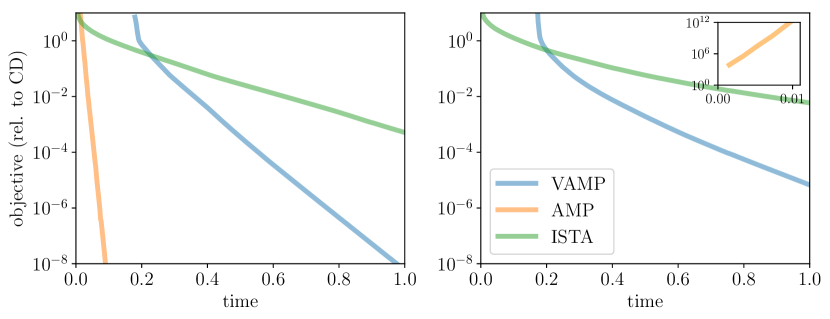
Figure 1: Comparison between AMP and VAMP for sparse regression on synthetic data, with $n=600$, $p=2000$ and $\rho=0.1$, $\sigma=10^{-5}$, $\lambda=1$. Objectives are relative to that of scikit-learn’s coordinate descent [30], which runs in a much shorter time (around $5\cdot 10^{-4}$s). Left: for Gaussian i.i.d. matrices, VAMP performs worse than AMP, both in terms of convergence rate and preprocessing time. Right: for a matrix which is not Gaussian i.i.d., but instead the product of two Gaussian i.i.d. matrices $\bm{A}=\bm{U}\bm{V}^{T}$, AMP quickly diverges, as shown in the inset, while VAMP keeps providing a good performance. In this example, both $\bm{U}$ and $\bm{V}$ have $r=600$ columns.

In order to compare the AMP iteration (2)-(3) to the VAMP one, (5)-(6), we perform a simple experiment on synthetic sparse data. We first sample $\bm{x}$ from a Bernoulli-Gaussian distribution, $P_{X}(\bm{x})=\prod_{j}[\rho\,\mathcal{N}(x_{j};0,1)+(1-\rho)\,\delta(x_{j})]$, then generate a matrix $\bm{A}$ by doing $\bm{A}_{ij}\sim\mathcal{N}(\bm{A}_{ij};0,1/n)$, to finally obtain measurements as $\bm{y}\sim\mathcal{N}(\bm{y};\bm{A}\bm{x},\sigma^{2}I_{n})$.

We try to recover $\bm{x}$ by using a $\ell_{1}$ penalty, $f(x_{j})=|x_{j}|$. In that case, $\eta_{\lambda\sigma^{t}}(x)=\Big{(}1-\frac{\lambda\sigma^{t}}{|x|}\Big{)}_{+}x$, also known as the soft thresholding operator. In Figure 1 (left), we study how fast each of the schemes performs this task. We look at three different schemes: iterative soft thresholding (ISTA) [31], the original AMP iteration (2)-(3), and the VAMP iteration (5)-(7). Compared to AMP and ISTA, VAMP has a larger preprocessing time, since it relies on the eigendecomposition of $\bm{A}\bm{A}^{T}$, as detailed in C. Moreover, in this artificial setting, its convergence rate is smaller than that of AMP.

Yet, such Gaussian matrices are precisely those assumed in the derivation of AMP. If a different matrix is used, say $\bm{A}=\bm{U}\bm{V}^{T}$ with both $\bm{U}$ and $\bm{V}$ Gaussian, then the AMP iteration quickly diverges, whereas VAMP continues to work (see Figure 1, right). One verifies in practice that VAMP converges for a broad class of matrices, and is actually proven to converge, in the large $n$ limit, for right orthogonally-invariant random matrices [14]. This motivates us to perform more detailed experiments with VAMP, as well as to adapt it to our needs.

Also notably, all schemes used in Figure 1 are much slower than coordinate descent, which is currently considered the state-of-the-art for optimization with separable penalties. For this reason, we shall consider the more interesting case of non-separable penalties in Section 3.

2.2 Variable splitting methods

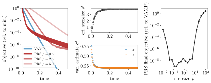
Figure 2: Comparison between VAMP and PRS algorithms for sparse regression on synthetic data, with $n=1200$, $p=2000$ and $\rho=0.2$, $\sigma^{2}=10^{-5}$, $\lambda=1$. Left: PRS behavior is highly dependent on the value chosen for the stepsize $\rho$, whereas for VAMP no parameter needs to be set. Center: effective stepsize (top) and variance estimates (bottom) provided by VAMP. Right: difference between PRS and VAMP objectives after 250 iterations.

We now turn to a class of optimization algorithms known as variable splitting methods. The main very basic idea is to minimize a sum of two functions such as (1) by writing each of them as a function of a different variable, and then enforcing these variables to assume the same value. This is done by means of the following augmented Lagrangian

$$\mathcal{L}(\bm{x},\bm{z},\bm{u})=\frac{1}{2}\|\bm{y}-\bm{A}\bm{x}\|_{2}^{2}+\lambda\sum_{j}f(z_{j})\underbrace{-\bm{u}^{T}(\bm{x}-\bm{z})+\frac{\rho}{2}\|\bm{x}-\bm{z}\|^{2}_{2}}_{\frac{\rho}{2}\|\bm{x}-\bm{z}-\frac{\bm{u}}{\rho}\|_{2}^{2}-\frac{1}{2\rho}\|\bm{u}\|_{2}^{2}},$$ (8)

One should minimize the expression above with respect to $\bm{x}$ and $\bm{z}$, and maximize its dual $\mathcal{L}^{\ast}=\min_{\bm{x},\bm{z}}\mathcal{L}(\bm{x},\bm{z},\bm{u})$ with respect to the Lagrange multiplier $\bm{u}$, see e.g. [32, 33]. The alternating direction method of multipliers (ADMM) [2, 3] accomplishes this by means of the following iteration

$$\bm{x}^{t}=\operatorname*{arg\,min\;}_{\bm{x}}\;\mathcal{L}(\bm{x},\bm{z}^{t},\bm{u}^{t})=\operatorname{prox}_{L/\rho}\,(\bm{z}^{t}+\nicefrac{{\bm{u}^{t}}}{{\rho}}),$$ (9)

$$\bm{z}^{t}=\operatorname*{arg\,min\;}_{\bm{z}}\;\mathcal{L}(\bm{x}^{t},\bm{z},\bm{u}^{t})=\operatorname{prox}_{R/\rho}\,(\bm{x}^{t}-\nicefrac{{\bm{u}^{t}}}{{\rho}}),$$ (10)

$$\bm{u}^{t+1}=\bm{u}^{t}+\rho(\bm{z}^{t}-\bm{x}^{t}).$$ (11)

where we have defined $L(\bm{x})=\frac{1}{2}\|\bm{y}-\bm{A}\bm{x}\|_{2}^{2}$ and $R(\bm{z})=\lambda\sum_{j}f(z_{j})$. Equations (9) and (10) perform two sequential gradient descent steps in $\mathcal{L}$, first for $\bm{x}$ then $\bm{z}$, whereas equation (11) is effectively a gradient ascent step in $\mathcal{L}^{\ast}(\bm{u})$, with stepsize set so as to satisfy the optimality conditions $\nabla_{\bm{x},\bm{z}}\mathcal{L}=0$.

The strategy employed by ADMM is empirically known as Douglas-Rachford splitting. Different strategies, with the same fixed points but slightly different updates, can be employed. For instance, the Peaceman-Rachford splitting (PRS) consists in the following equations [34, 35]

$$\bm{x}^{t}=\operatorname{prox}_{L/\rho}\;(\nicefrac{{\bm{u}^{t}}}{{\rho}}),$$ (12)

$$\bm{z}^{t}=\operatorname{prox}_{R/\rho}\;(2\bm{x}^{t}-\nicefrac{{\bm{u}^{t}}}{{\rho}}),$$ (13)

$$\bm{u}^{t+1}=\bm{u}^{t}+2\rho(\bm{z}^{t}-\bm{x}^{t}).$$ (14)

While PRS is known to often lead to lower objectives faster than ADMM [34, 36], it is provably convergent under stronger assumptions, and in practice the objective often does not decrease monotonically.

Writing the proximal operators explicitly in the PRS iteration (12) and (13) yields

$$\bm{x}^{t}=(\bm{A}^{T}\bm{A}+\rho I_{n})^{-1}(\bm{A}^{T}\bm{y}+\bm{u}^{t}),\kern 40.00006pt\bm{z}^{t}=\eta_{\lambda/\rho}(2\bm{x}^{t}-\bm{u}^{t}/\rho).$$ (15)

Interestingly, setting $\sigma_{x}^{t}=\sigma_{z}^{t}=\frac{1}{2\rho}$ in the VAMP iteration (5)-(6) leads to the PRS iteration above; VAMP can thus be seen as a PRS variant where the stepsize is set adaptively. This remark has been first made in [37].

We thus see that VAMP is more robust than AMP, converging in situations where AMP does not, as shown in Figure 1. It also has a significant advantage over variable-splitting methods, since no stepsize needs to be set. While neither VAMP nor variable-splitting methods are competitive with the state-of-the-art in the particular setting of separable penalties, we now turn to non-sperable penalties, which are more challenging regarding efficiency and convergence control [38], yet very important in practical applications.

3 Non-separable penalties

Consider a penalty which is separable not on $\bm{x}$ but on disjoint subsets of a linear transformation $\bm{K}\bm{x}$, with $\bm{K}\in\mathbb{R}^{r\times n}$

$$\hat{\bm{x}}=\operatorname*{arg\,min\;}_{\bm{x}}\frac{1}{2}\|\bm{y}-\bm{A}\bm{x}\|_{2}^{2}+\lambda\sum_{k=1}^{r}f\big{(}(\bm{K}\bm{x})_{k}\big{)},$$ (16)

for any convex function $f$. Note that $k$ does not necessarily index a single component of $\bm{K}\bm{x}$, but more generally a subset of components; moreover, each component belongs to a single subset. An example is the so-called total variation (TV) penalty [18, 19], used to enforce spatial regularity – typically flat regions separated by sharp transitions

$$R_{\rm TV}(\bm{x})=\sum_{ij}\sqrt{(x_{i,j}-x_{i,j-1})^{2}+(x_{i,j}-x_{i-1,j})^{2}},$$ (17)

where we have indexed the vector $\bm{x}$ by two components $i,j$ such that $x_{k}=x_{i,j}$ for $i=\lfloor k/L\rfloor$ and $j=k\mod L$. By defining a gradient operator $\nabla$

$$(\nabla\bm{x})_{k}=\begin{pmatrix}x_{i,j+1}-x_{i,j}\\ x_{i+1,j}-x_{i,j}\end{pmatrix},$$ (18)

the 2D TV penalty can be conveniently written as $R_{\rm TV}=\sum_{k=1}^{2n}\|(\nabla\bm{x})_{k}\|_{2}\equiv\|\nabla\bm{x}\|_{2,1}$. Different boundary conditions can be used; in our experiments, we assume periodic boundary conditions.

While we define it above for two dimensions, the TV operator is easily generalizated to lattices in three or more dimensions. Notice moreover that we are dealing with the isotropic or rotation-invariant TV operator, instead of the anisotropic one $\|\nabla\bm{x}\|_{1,1}$.

Variable splitting algorithms can be easily adapted to that case, by using a split variable $\bm{z}=\bm{K}\bm{x}$; the augmented Lagrangian (8) becomes

$$\mathcal{L}(\bm{x},\bm{z},\bm{u})=\frac{1}{2}\|\bm{y}-\bm{A}\bm{x}\|_{2}^{2}+\lambda\sum_{k=1}^{r}f(z_{k})-\bm{u}^{T}(\bm{K}\bm{x}-\bm{z})+\frac{\rho}{2}\|\bm{K}\bm{x}-\bm{z}\|^{2}_{2}.$$ (19)

and the PRS iteration is now written

$$\bm{x}^{t}=(\bm{A}^{T}\bm{A}+\rho\bm{K}^{T}\bm{K})^{-1}(\bm{A}^{T}\bm{y}+\bm{K}^{T}\bm{u}^{t}),$$ (20)

$$\bm{z}^{t}=\eta_{\lambda/\rho}(2\bm{K}\bm{x}^{t}-\bm{u}^{t}/\rho),$$ (21)

$$\bm{u}^{t+1}=\bm{u}^{t}+2\rho(\bm{z}^{t}-\bm{K}\bm{x}^{t}).$$ (22)

In particular for TV, $\bm{K}=\nabla$ and the $\eta$ function is given by the group soft thresholding operator

$$\eta_{\lambda/\rho}(\bm{v})=\bigg{(}1-\frac{\lambda/\rho}{\|\bm{v}\|_{2}}\bigg{)}_{+}\,\bm{v}.$$ (23)

3.1 VAMP for non-separable penalties

The following VAMP-like iteration, which we derive in B, can be used in order to solve problem 16

$$\bm{x}^{t}=(\bm{A}^{T}\bm{A}+\rho^{t}\bm{K}^{T}\bm{K})^{-1}(\bm{A}^{T}\bm{y}+\bm{K}^{T}\bm{u}^{t}), \sigma^{t}_{x}=\frac{1}{n}\Tr\big{[}\bm{K}(\bm{A}^{T}\bm{A}+\rho^{t}\bm{K}^{T}\bm{K})^{-1}\bm{K}^{T}\big{]},$$ (24)

$$\bm{z}^{t}=\eta_{\frac{\lambda\sigma_{x}^{t}}{1-\sigma_{x}^{t}\rho^{t}}}\bigg{(}\frac{\bm{K}\bm{x}^{t}-\sigma_{x}^{t}\bm{u}^{t}}{1-\sigma_{x}^{t}\rho^{t}}\bigg{)}, \sigma^{t}_{z}=\frac{\sigma_{x}^{t}}{1-\sigma_{x}^{t}\rho^{t}}\,\bigg{\langle}\nabla\eta_{\frac{\lambda\sigma_{x}^{t}}{1-\sigma_{x}^{t}\rho^{t}}}\bigg{(}\frac{\bm{K}\bm{x}^{t}-\sigma_{x}^{t}\bm{u}^{t}}{1-\sigma_{x}^{t}\rho^{t}}\bigg{)}\bigg{\rangle},$$ (25)

$$\bm{u}^{t+1}=\bm{u}^{t}+(\bm{z}^{t}/\sigma_{z}^{t}-\bm{K}\bm{x}^{t}/\sigma_{x}^{t}), \rho^{t+1}=\rho^{t}+(1/\sigma^{t}_{z}-1/\sigma^{t}_{x}).$$ (26)

Upon convergence, it is verified that $\bm{z}=\bm{K}\bm{x}$ and $\sigma_{x}=\sigma_{z}$. Once again, if the variances remain fixed throughout the iteration, $\sigma_{x}^{t}=\sigma_{z}^{t}=\frac{1}{2\rho}$, the PRS iteration (20)-(22) is recovered. Moreover, the Woodbury formula can also be applied, leading to a faster iteration whenever $n\ll p$. The iteration is particularly fast for the TV matrix $\bm{K}=\nabla$, for which $\bm{K}^{T}\bm{K}=\Delta$ is a circulant matrix and thus diagonal in the Fourier basis, see C.1.

While we consider convex $f$ functions, we never use this assumption explicitly. In other words, the iteration above could, in principle, also be used when $f$ is non-convex.

3.2 Enforcing contractivity

A well-known issue with PRS is that, differently from ADMM, the iteration mapping might not be contractive [39, 36], which might lead to lack of convergence. The iteration we propose, (24)-(26), suffers from the same issue. A way of enforcing contractivity, done for PRS in [36], is by including a underdetermined relaxation factor $0<\gamma<1$ in the update of the Lagrange multiplier $\bm{u}$, that is

$$\bm{u}^{t+1}=\bm{u}^{t}+\gamma(\bm{z}^{t}/\sigma_{z}^{t}-\bm{K}\bm{x}^{t}/\sigma_{x}^{t}).$$ (27)

For consistency, we also include the same parameter in the update of the stepsize $\rho$

$$\rho^{t+1}=\rho^{t}+\gamma(1/\sigma_{z}^{t}-1/\sigma_{x}^{t}).$$ (28)

While this modification improves the convergence properties of the algorithm, it also makes us need to specify an extra parameter $\gamma$. This parameter could in principle be set adaptively, as it has been done for other AMP algorithms [27]. In our experiments, however, we leave this parameter fixed at a small enough value chosen arbitrarily, $\gamma=0.6$.

4 Numerical experiments

In this section we solve problem (16) for a 2D total variation penalty, $\bm{K}=\nabla$, and different choices of $\{\bm{y},\bm{A}\}$. We compare the iteration we propose, (24)-(26), to three other standard algorithms: ADMM with an adaptive stepsize [40]; a FISTA [1] adaptation known as FAASTA [41], as implemented in the Nilearn package [42]; and the Peaceman-Rachford splitting, recovered by leaving variances fixed in our own implementation.

We work in the high-dimensional regime with $n\ll p$ and thus use the numerical tricks described in C, combining the Woodbury formula to the eigendecompositions of $\bm{A}\bm{A}^{T}$ and $\bm{K}^{T}\bm{K}$ to speed up the evaluation of the proximal step in VAMP, PRS and ADMM. In all experiments, we set the relaxation factor to $\gamma=0.6$ in VAMP, and to $\gamma=0.95$ in PRS.

All experiments have been performed on a machine with a 12-core Intel i7-8700K processor and 32GB of RAM, using Numpy and a multi-CPU implementation of BLAS (OpenBLAS).

4.1 Classification in task fMRI

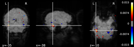
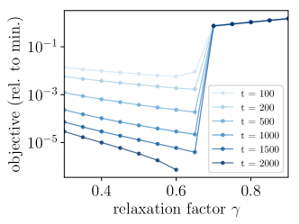
Figure 3: Left: weight map obtained by VAMP in classifying “face” vs. all. Intensities are thresholded at 0.002. Right: objective in classifying “face” vs. all at different numbers of iterations, for different choices of relaxation factor. If the relaxation factor is set small enough, there is no noticeable difference in performance.

In our first numerical experiment, we approach a multi-class classification problem, namely a task fMRI one: each row of $\bm{A}\in\mathbb{R}^{n\times p}$ is given by an fMRI image, while the entries of $\bm{y}\in\mathbb{R}^{n}$ tell us what task was being performed by the subject at the time of acquisition. We use the Haxby dataset [43], which is commonly used for benchmarks and contains $n=1452$ samples of $p=40\times 64\times 64=163840$ features each. The classes refer to what image the subject was observing at the time of acquisition. We perform one vs. all classification for three of these classes: “face”, “house” and “chair”, each associated to 108 of the 1452 samples.

While $p=163840$, many of the voxels are zero-valued and thus a mask can be applied, leading to a new feature matrix with only $39912$ columns. One can pass this smaller matrix to FISTA instead of the full one, as it is capable of dealing with such masks. However, the remaining methods require the full matrix, at least in the way we have implemented them.

Two of the parameters are fixed: the regularization $\lambda=0.1$ and the relaxation $\gamma$, which is set to 0.6 for VAMP and to 0.95 for PRS. In this setting, VAMP achieves smaller values of the objective faster than all other methods and for all the three classes considered, as shown in Figure 4. The weight map obtained in “face” classification is displayed in Figure 3.

In Figure 3 (right), we study how the performance of our scheme changes in this experiment as a function of $\gamma$. We can see the performance does not change considerably as long as $\gamma$ is set small enough. While this has been often observed by us, further experiments must be performed to ensure such behavior is indeed recurrent. If that is the case, it should be straightforward to devise an adaptive scheme for $\gamma$.

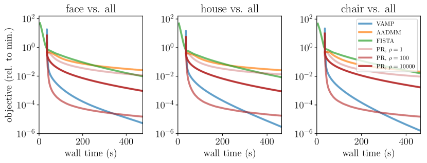
Figure 4: Classification in task fMRI using the Haxby dataset, $n=1452$ and $p=136840$. Since there are multiple classes, we perform one vs. all classification for three specific ones: “face”, “house” and “chair”. All schemes seek to solve the same convex optimization problem (16) with a TV penalty, $\bm{K}=\nabla$, and $\lambda=0.1$. For all three classes considered, VAMP achieves a lower objective faster than all other schemes. VAMP, AADMM and PR have a late start due to preprocessing time, during which the eigendecomposition of $\bm{A}^{T}\bm{A}$ is evaluated.

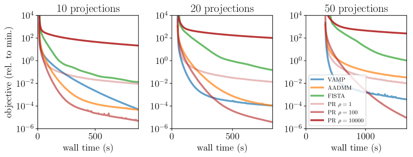
Figure 5: Reconstruction of a Sheep-Logan phantom of size 200x200 ($p=40000$) using 10 (left), 20 (center) and 50 (right) equally spaced noisy projections ($n=2000$, $4000$ and $10000$, respectively). A TV penalty is used with $\lambda=1.0$. For 10 and 20 projections, VAMP and AADMM are competitive with each other and both faster than FISTA; for 50 projections, VAMP seems to be considerably faster. Meanwhile, PRS performance is highly dependent on the choice of the stepsize $\rho$. Note that preprocessing time is not discounted for any of the approaches, and that a larger number of projections (i.e. larger $n$) incurs bigger preprocessing times.

4.2 Reconstruction in tomography

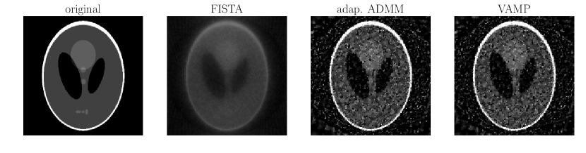
Figure 6: Estimates obtained by the different approaches 10 seconds after preprocessing is finished, using 50 noisy projections.

A second experiment consists in reconstructing a two-dimensional image from a number of tomographic projections. We use a Shepp-Logan phantom of dimensions 200x200, so that $p=40000$, and perform the reconstruction for 10 ($n=2000$), 20 ($n=4000$) and 50 ($n=10000$) equally spaced projections. Moreover, we add a 1% SNR noise to the projections. In other words, the tomographic projections are generated as $\bm{y}=\bm{A}\bm{x}+\mathcal{N}(0,\sigma^{2})$, where $\bm{A}$ is the two-dimensional Radon transform and $\sigma^{2}=0.01\cdot\|\bm{A}\bm{x}\|_{2}^{2}/n$. In our experiments, we explicitly generate the Radon matrix, that is, we do not use its operator form.

The regularization parameter is set to $\lambda=1.0$, and the relaxation parameter to $\gamma=0.6$. While for the reconstruction using 20 and 50 projections VAMP is faster than the remaining algorithms, for 10 projections it is beaten by adaptive-step ADMM, being, however, still competitive with FISTA. Finally, we show the performance of Peaceman-Rachford for different values of stepsize $\rho$; while it might eventually perform better than all the other algorithms, its behaviour is highly dependant on the choice of stepsize.

5 Conclusion

We have proposed a VAMP-like iteration for optimizing functions consisting of linear losses and a given class of non-separable penalties. As the usual VAMP iteration, it can be seen as a Peaceman-Rachford splitting with adaptive stepsizes. Initial experiments reveal that the resulting algorithm is competitive with, and faster than other typically employed optimization schemes, namely ADMM and FISTA. While further experiments should be performed in order to assess the superiority of the algorithm in more general settings, we believe that the results displayed demonstrate its potential for real-world applications.

Our analysis also elucidates the connection between message-passing algorithms and other known optimization schemes, expanding on the remark of [37]. In particular, the Peaceman-Rachford splitting is recovered if variances/stepsizes are kept fixed. Further exploring this connection should lead to improved inference and optimization algorithms, and hopefully also to convergence proofs, which are typically difficult to obtain for message-passing algorithms.

There are other EC/VAMP adaptations able to deal with constraints of the form $\bm{z}=\bm{K}\bm{x}$, but these are typically used on the loss, not the penalty [44, 45]. They could be integrated into our framework to study losses other than quadratic. An alternative would be using these adaptations on the penalty instead, by artificially introducing new effective samples that mimic the penalty as an additional loss term; this has been explored for AMP in [46, 47], and is not as straightforward as the construction we use in this paper.

Yet another perspective is adapting the algorithm for online inference, using the scheme described in [48]. Interestingly, this is similar to what is already done to adapt ADMM to the online setting [49]. Finally, we leave for future work comparing our approach to other recent promising alternatives, in particular that of [50].

Appendix A Expectation-consistent approximation

The expectation-consistent approximation[23] is defined for a probability distribution of the form

$$P(\bm{x})=\frac{1}{\mathcal{Z}}P_{\ell}(\bm{x})\,P_{r}(\bm{x}).$$ (29)

It seeks to approximate (minus) the log-partition function $-\log\mathcal{Z}=-\log\int d\bm{x}\,P_{\ell}(\bm{x})\,P_{r}(\bm{x})$ by means of the following objective, denoted the expectation-consistent free energy

$$\mathcal{F}[Q_{\ell},Q_{r}]=-\log\int d\bm{x}\,P_{\ell}(\bm{x})\,Q_{r}(\bm{x})-\log\int d\bm{x}\,Q_{\ell}(\bm{x})\,P_{r}(\bm{x})+\log\int d\bm{x}\,Q_{\ell}(\bm{x})\,Q_{r}(\bm{x}).$$ (30)

If there are no restrictions on $Q$, then $\mathcal{F}$ is minimized for $Q_{\ell}=P_{\ell}$, $Q_{r}=P_{r}$. What we want however is to have a tractable approximation, so the $Q$ are typically replaced by distributions in the exponential family. We use a (unnormalized) Gaussian distribution, written in canonical form as

$$Q_{\ell,r}(\bm{x})=e^{-\frac{1}{2}\rho_{\ell,r}\bm{x}^{T}\bm{x}+\bm{u}_{\ell,r}^{T}\bm{x}}.$$ (31)

In our case, $P_{\ell}(\bm{x})\propto e^{-\frac{1}{2}\|\bm{y}-\bm{A}\bm{x}\|_{2}^{2}}$ and $P_{r}(\bm{x})=\prod_{j=1}^{p}e^{-\lambda f(x_{j})}$. Combined to the explicit form of $Q$ above this gives

$$\mathcal{F}(\bm{u}_{\ell},\bm{u}_{r},\rho_{\ell},\rho_{r})=\frac{1}{2}\bm{y}^{T}\bm{y}-\frac{1}{2}(\bm{A}^{T}\bm{y}+\bm{u}_{r})^{T}(\bm{A}^{T}\bm{A}+\rho_{r}I_{p})^{-1}(\bm{A}^{T}\bm{y}+\bm{u}_{r})+$$ (32)

$$\kern 50.00008pt+\frac{1}{2}\log\det(\rho_{r}I_{p}+\bm{A}^{T}\bm{A})-\sum_{j=1}^{p}\log\int dx_{j}e^{-\lambda f(x_{j})}e^{-\frac{1}{2}\rho_{\ell}x_{j}^{2}+u_{\ell k}x_{j}}+$$

$$\kern 50.00008pt+\frac{1}{2}\sum_{j=1}^{p}\left[\frac{u_{rk}+u_{\ell k}}{\rho_{r}+\rho_{\ell}}-\log(\rho_{r}+\rho_{\ell})\right].$$

There are different ways of looking for local minima of $\mathcal{F}$ [23]; the vector AMP iteration [14] is one of them. It consists in the following fixed-point iteration

$$\bm{u}_{\ell}^{t+1}=\frac{\mathbb{E}_{\ell}^{t}\bm{x}}{\langle\operatorname{Var}_{\ell}^{t}(\bm{x})\rangle}-\bm{u}_{r}^{t},\qquad\rho_{\ell}^{t+1}=\frac{1}{\langle\operatorname{Var}_{\ell}^{t}(\bm{x})\rangle}-\rho_{r}^{t},$$ (33)

$$\bm{u}_{r}^{t+1}=\frac{\mathbb{E}_{r}^{t}\bm{x}}{\langle\operatorname{Var}_{r}(\bm{x})\rangle}-\bm{u}_{\ell}^{t},\qquad\rho_{r}^{t+1}=\frac{1}{\langle\operatorname{Var}_{r}^{t}(\bm{x})\rangle}-\rho_{\ell}^{t},$$

where we denote by $\mathbb{E}_{\ell,r}^{t}$ the expectation w.r.t. the tilted distributions $\tilde{Q}_{\ell,r}^{t}(\bm{x})\propto P_{\ell,r}(\bm{x})Q_{\ell,r}^{t}(\bm{x})$, and by $\operatorname{Var}_{r,\ell}^{t}(\bm{x})$ the variance of these distributions. In particular

$$\mathbb{E}_{\ell}^{t}\bm{x}=(\bm{A}^{T}\bm{A}+\rho_{r}^{t}I_{p})^{-1}(\bm{A}^{T}\bm{y}+\bm{u}_{r}^{t}),\qquad\langle\operatorname{Var}_{\ell}^{t}(\bm{x})\rangle=\frac{1}{p}\Tr(\bm{A}^{T}\bm{A}+\rho_{r}^{t}I_{p})^{-1},$$ (34)

and, by defining $z(u,\rho)=\int dxe^{-\lambda f(x)}e^{-\frac{1}{2}\rho x^{2}+ux}$,

$$\mathbb{E}_{r}^{t}x_{j}=\frac{\partial}{\partial u}\log z(u,\rho)\Big{|}_{u_{\ell k}^{t},\rho_{\ell}^{t}},\qquad\langle\operatorname{Var}_{r}^{t}(\bm{x})\rangle=\frac{1}{p}\sum_{j=1}^{p}\frac{\partial^{2}}{\partial u^{2}}\log z(u,\rho)\Big{|}_{u_{\ell k}^{t},\rho_{\ell}^{t}},$$ (35)

Note that upon convergence one achieves the stationary conditions $\nabla\mathcal{F}=0$

$$\bm{u}_{\ell}+\bm{u}_{r}=\frac{\mathbb{E}_{\ell}\bm{x}}{\langle\operatorname{Var}_{\ell}(\bm{x})\rangle}=\frac{\mathbb{E}_{r}\bm{x}}{\langle\operatorname{Var}_{r}(\bm{x})\rangle},\qquad\rho_{\ell}+\rho_{r}=\frac{1}{\langle\operatorname{Var}_{\ell}(\bm{x})\rangle}=\frac{1}{\langle\operatorname{Var}_{r}(\bm{x})\rangle}.$$ (36)

In other words, the first two moments of $\tilde{Q}_{\ell}$ and $\tilde{Q}_{r}$ must be consistent with those of the approximating posterior $Q(\bm{x})\propto Q_{\ell}(\bm{x})Q_{r}(\bm{x})$.

A.1 MAP estimate

In order to go from the equations above to (5)-(7), we perform two additional steps. First, note that one does not need to work with both $\ell$ and $r$ variables; by denoting $\bm{u}\equiv\bm{u}_{r}$, we rewrite the iteration as

$$\bm{u}^{t+1}=\bm{u}^{t}+\left(\frac{\mathbb{E}_{r}^{t}\bm{x}}{\langle\operatorname{Var}_{r}^{t}(\bm{x})\rangle}-\frac{\mathbb{E}_{\ell}^{t}\bm{x}}{\langle\operatorname{Var}_{\ell}^{t}(\bm{x})\rangle}\right),$$ (37)

and analogously for $\rho$, thus obtaining (6). Moreover, since we are interested in the MAP estimate, we use the following trick: we consider instead a distribution $P(\bm{x})\propto[P_{\ell}(\bm{x})\,P_{r}(\bm{x})]^{\beta}$ and take the limit $\beta\to\infty$, thus making the distribution concentrate around its mode; we then look at $\frac{1}{\beta}\log\mathcal{Z}$. By rescaling $\bm{u}_{\ell,r}\to\beta\bm{u}_{\ell,r}$ and $\rho_{\ell,r}\to\beta\rho_{\ell,r}$, we ensure that most equations remain the same. The only difference is in the second integral in $\mathcal{F}$, which can be performed using the Laplace method to yield

$$\frac{1}{\beta}\log z(u,\rho)=\frac{1}{\beta}\log\int dx_{j}e^{-\beta\left\{\lambda f(x)+\frac{1}{2}\rho x-ux\right\}}\xrightarrow{\beta\to\infty}\frac{u^{2}}{2\rho}-\rho\mathcal{M}_{\lambda f/\rho_{\ell}}(u/\rho),$$ (38)

where $\mathcal{M}_{f}(v)=\min_{x}\Big{\{}f(x)+\frac{1}{2}(x-v)^{2}\Big{\}}$ is the Moreau envelope of $f$. Given that $\frac{\partial}{\partial v}\mathcal{M}_{f}(v)=x-\operatorname{prox}_{f}(v)$, we get using (35) that

$$\mathbb{E}_{r}^{t}\bm{x}=\operatorname{prox}_{\lambda f/\rho_{\ell}^{t}}(\bm{u}_{\ell}/\rho_{\ell})\equiv\eta_{\lambda f/\rho_{\ell}^{t}}(\bm{u}_{\ell}/\rho_{\ell}),$$ (39)

and also that $\langle\operatorname{Var}_{r}^{t}(\bm{x})\rangle=\rho_{\ell}^{-1}\langle\nabla\eta_{\lambda f/\rho_{\ell}^{t}}(\bm{u}_{\ell}/\rho_{\ell})\rangle$, leading to (5) and (7).

Appendix B Adapting the EC approximation to TV penalties

In order to adapt iteration (5)-(6) to total variation penalties, we look at the expectation-consistent (EC) approximation [23] in closer detail. We first define the following distribution

$$P(\bm{x})\propto e^{-\frac{1}{2}\|\bm{y}-\bm{A}\bm{x}\|_{2}^{2}}\,\prod_{k=1}^{r}e^{-\lambda f\big{(}(\bm{K}\bm{x})_{k}\big{)}}.$$ (40)

Problem (16) is then recovered when considering the MAP estimator for $\bm{x}$, given by the mode of $P(\bm{x})$. Next we introduce a variable $\bm{z}=\bm{K}\bm{x}$, and rewrite the distribution above as

$$P(\bm{x},\bm{z})\propto e^{-\frac{1}{2}\|\bm{y}-\bm{A}\bm{x}\|_{2}^{2}}\,\delta(\bm{z}-\bm{K}\bm{x})\prod_{k=1}^{r}e^{-\lambda f\big{(}z_{k}\big{)}}.$$ (41)

so that the marginal distribution of $\bm{z}$ becomes

$$P(\bm{z})=\frac{1}{\mathcal{Z}}\,\bigg{[}\!\int d\bm{x}\,e^{-\frac{1}{2}\|\bm{y}-\bm{A}\bm{x}\|_{2}^{2}}\,\delta(\bm{z}-\bm{K}\bm{x})\bigg{]}\,\prod_{k=1}^{r}e^{-\lambda f(z_{k})}.$$ (42)

We apply the EC scheme described above for $P(\bm{z})$, by setting

$$P_{\ell}(\bm{z})\propto\int d\bm{x}\,e^{-\frac{1}{2}\|\bm{y}-\bm{A}\bm{x}\|_{2}^{2}}\,\delta(\bm{z}-\bm{K}\bm{x}),\qquad P_{r}(\bm{z})\propto\prod_{k=1}^{r}e^{-\lambda f(z_{k})},$$ (43)

thus yielding the following expectation-consistent free energy

$$\mathcal{F}[Q_{\ell},Q_{r}]=-\log\int d\bm{x}\,e^{-\frac{1}{2}\|\bm{y}-\bm{A}\bm{x}\|_{2}^{2}}\,Q_{r}(\bm{K}\bm{x})-\log\int d\bm{z}\,Q_{\ell}(\bm{z})P_{r}(\bm{z})+\log\int d\bm{z}\,Q_{\ell}(\bm{z})Q_{r}(\bm{z}),$$ (44)

We once again parametrize these distributions by canonical-form Gaussians, $Q_{\ell,r}(\bm{z};\bm{u}_{\ell,r},\rho_{\ell,r})=e^{-\frac{\rho_{\ell,r}}{2}\bm{z}^{T}\bm{z}+\bm{u}_{\ell,r}^{T}\bm{z}}$, leading to the fixed-point iteration (24)-(26).

Appendix C VAMP iteration for $n\ll p$

In the $n\ll p$ setting, iteration (5) can be made efficient by combining the Woodbury formula with the eigendecomposition of $\bm{A}\bm{A}^{T}=\bm{U}\operatorname{diag}(\bm{d})\bm{U}^{T}$. We first use the Woodbury formula to replace the iteration on $\bm{x}$ by

$$\bm{x}^{t}=\frac{\bm{u}^{t}}{\rho^{t}}+\bm{A}^{T}(\bm{A}\bm{A}^{T}+\rho^{t}I_{n})^{-1}\bigg{(}y-\bm{A}\frac{\bm{u}^{t}}{\rho^{t}}\bigg{)},$$ (45)

and then insert the eigendecomposition

$$\bm{x}^{t}=\frac{\bm{u}^{t}}{\rho^{t}}+\bm{A}^{T}\bm{U}\bigg{\{}\bigg{[}\bm{U}^{T}\bigg{(}y-\bm{A}\frac{\bm{u}^{t}}{\rho^{t}}\bigg{)}\bigg{]}\oslash(\bm{d}+\rho^{t})\bigg{\}},$$ (46)

where we have used the symbol $\oslash$ to denote the Hadamard or elementwise division between two vectors. Note that evaluating the expression above consists only in performing matrix-vector products and other vector-vector operations, and can thus be performed in $O(np)$.

Finally, iteration (7) can be replaced by

$$\sigma_{x}^{t}=\frac{1}{n}\sum_{i=1}^{n}\frac{1}{d_{i}+\rho^{t}}.$$ (47)

C.1 Further simplifications for TV penalty

For the non-separable penalty (16), the same trick can be applied to yield

$$\bm{x}^{t}=(\bm{K}^{T}\bm{K})^{-1}\frac{\bm{u}^{t}}{\rho^{t}}+(\bm{K}^{T}\bm{K})^{-1}\bm{A}^{T}\bm{U}\bigg{\{}\bigg{[}\bm{U}^{T}(\bm{y}-\bm{A}(\bm{K}^{T}\bm{K})^{-1}\frac{\bm{u}^{t}}{\rho^{t}}\bigg{]}\oslash(\bm{d}+\rho^{t})\bigg{\}},$$ (48)

and, by further using the eigendecomposition of $\bm{K}^{T}\bm{K}=\bm{F}^{T}\bm{\Lambda}\bm{F}$

$$\bm{x}^{t}=\bm{F}^{T}\bm{\Lambda}^{-1}\Bigg{\{}\bm{F}\frac{\bm{u}^{t}}{\rho^{t}}+\tilde{\bm{A}}^{T}\bm{U}\bigg{\{}\bigg{[}\bm{U}^{T}(\bm{y}-\tilde{\bm{A}}\bm{\Lambda}^{-1}\bm{F}\frac{\bm{u}^{t}}{\rho^{t}}\bigg{]}\oslash(\bm{d}+\rho^{t})\bigg{\}}\Bigg{\}},$$ (49)

for $\tilde{\bm{A}}^{T}=\bm{F}\bm{A}^{T}$. In particular for the TV penalty, $\bm{K}=\nabla$ is the gradient operator and $\bm{K}^{T}\bm{K}=\Delta$ is the Laplacian, which being a circulant matrix has $\bm{F}$ given by the Fourier transform. We can then replace $\bm{F}$ by the FFT, so that the expression above can be evaluated almost as efficiently as (46).

The iteration on $\sigma_{x}$ is written in this case as

$$\sigma_{x}^{t}=\frac{1}{\rho^{t}}\left[\frac{1}{d}-\frac{1}{nd}\sum_{i=1}^{nd}\frac{d_{i}}{d_{i}+\rho^{t}}\right]=\frac{1}{nd}\sum_{i=1}^{nd}\frac{1}{d_{i}+\rho^{t}}-\frac{d-1}{d}\frac{1}{\rho^{t}},$$ (50)

where $d$ is the dimension of the TV operator, i.e. $\bm{K}=\nabla$ is a $nd\times n$ matrix.

References

References

- [1] Beck A and Teboulle M 2009 SIAM Journal on Imaging Sciences 2 183–202
- [2] Boyd S, Parikh N, Chu E, Peleato B and Eckstein J 2011 Foundations and Trends in Machine Learning 3 1–122
- [3] Douglas J and Rachford H H 1956 Transactions of the American Mathematical Society 82 421–439
- [4] Donoho D L, Maleki A and Montanari A 2009 Proceedings of the National Academy of Sciences 106 18914–18919
- [5] Rangan S 2011 Generalized approximate message passing for estimation with random linear mixing IEEE International Symposium on Information Theory (ISIT) pp 2168–2172
- [6] Krzakala F, Mézard M, Sausset F, Sun Y and Zdeborová L 2012 Physical Review X 2 021005
- [7] Pearl J 1988 Probabilistic reasoning in intelligent systems: networks of plausible inference (Morgan Kaufmann)
- [8] Vila J P and Schniter P 2013 IEEE Transactions on Signal Processing 61 4658–4672
- [9] Ziniel J, Schniter P and Sederberg P 2014 Binary linear classification and feature selection via generalized approximate message passing Information Sciences and Systems (CISS), 2014 48th Annual Conference on (IEEE) pp 1–6
- [10] Guo C and Davies M E 2015 IEEE Transactions on Signal Processing 63 2130–2141
- [11] Metzler C A, Maleki A and Baraniuk R G 2016 IEEE Transactions on Information Theory 62 5117–5144
- [12] Rangan S, Schniter P and Fletcher A 2014 On the convergence of approximate message passing with arbitrary matrices IEEE International Symposium on Information Theory (ISIT) pp 236–240
- [13] Caltagirone F, Zdeborová L and Krzakala F 2014 On convergence of approximate message passing IEEE International Symposium on Information Theory (ISIT) pp 1812–1816
- [14] Rangan S, Schniter P and Fletcher A K 2017 Vector approximate message passing IEEE International Symposium on Information Theory (ISIT) pp 1588–1592
- [15] Reeves G and Pfister H D 2016 The replica-symmetric prediction for compressed sensing with Gaussian matrices is exact IEEE International Symposium on Information Theory (ISIT)
- [16] Barbier J, Krzakala F, Macris N, Miolane L and Zdeborová L 2017 arXiv:1708.03395
- [17] Barbier J, Macris N, Maillard A and Krzakala F 2018 The Mutual Information in Random Linear Estimation Beyond i.i.d. Matrices IEEE International Symposium on Information Theory (ISIT)
- [18] Beck A and Teboulle M 2009 IEEE Transactions on Image Processing 18 2419–2434
- [19] Michel V, Gramfort A, Varoquaux G, Eger E and Thirion B 2011 IEEE Transactions on Medical Imaging 30 1328–1340
- [20] Parikh N and Boyd S 2014 Foundations and Trends in Optimization 1 127–239
- [21] Fletcher A K, Rangan S, Sarkar S and Schniter P 2018 arXiv preprint arXiv:1806.10466
- [22] Schniter P, Rangan S and Fletcher A 2017 Denoising based vector approximate message passing Proc. Intl. Biomedical and Astronomical Signal Process. (BASP) Workshop p 77
- [23] Opper M and Winther O 2005 Journal of Machine Learning Research 6 2177–2204
- [24] Donoho D L, Maleki A and Montanari A 2010 Message passing algorithms for compressed sensing: I. motivation and construction IEEE Information Theory Workshop (ITW) (IEEE) pp 1–5
- [25] Thouless D J, Anderson P W and Palmer R G 1977 Philosophical Magazine 35 593–601
- [26] Mézard M 1989 Journal of Physics A: Mathematical and General 22 2181
- [27] Vila J, Schniter P, Rangan S, Krzakala F and Zdeborová L 2015 Adaptive damping and mean removal for the generalized approximate message passing algorithm IEEE International Conference on Acoustics, Speech and Signal Processing (ICASSP) pp 2021–2025
- [28] Manoel A, Krzakala F, Tramel E and Zdeborová L 2015 Swept approximate message passing for sparse estimation International Conference on Machine Learning (ICML) pp 1123–1132
- [29] Ma J and Ping L 2017 IEEE Access 5 2020–2033
- [30] Pedregosa F, Varoquaux G, Gramfort A, Michel V, Thirion B, Grisel O, Blondel M, Prettenhofer P, Weiss R, Dubourg V, Vanderplas J, Passos A, Cournapeau D, Brucher M, Perrot M and Duchesnay E 2011 Journal of Machine Learning Research 12 2825–2830
- [31] Donoho D L 1995 IEEE Transactions on Information Theory 41 613–627
- [32] Boyd S and Vandenberghe L 2004 Convex optimization (Cambridge University Press)
- [33] Nocedal J and Wright S J 2006 Numerical optimization 2nd ed (Springer)
- [34] Gabay D 1983 Applications of the method of multipliers to variational inequalities Studies in Mathematics and its Applications vol 15 (Elsevier) pp 299–331
- [35] Peaceman D W and Rachford Jr H H 1955 Journal of the Society for industrial and Applied Mathematics 3 28–41
- [36] He B, Liu H, Wang Z and Yuan X 2014 SIAM Journal on Optimization 24 1011–1040
- [37] Fletcher A, Sahraee-Ardakan M, Rangan S and Schniter P 2016 Expectation consistent approximate inference: Generalizations and convergence IEEE International Symposium on Information Theory (ISIT) pp 190–194
- [38] Dohmatob E, Gramfort A, Thirion B and Varoquaux G 2014 Benchmarking solvers for tv- least-squares and logistic regression in brain imaging International Workshop on Pattern Recognition in Neuroimaging (IEEE) pp 1–4
- [39] He B, Liao L Z, Han D and Yang H 2002 Mathematical Programming 92 103–118
- [40] Xu Z, Figueiredo M and Goldstein T 2017 Adaptive ADMM with spectral penalty parameter selection International Conference on Artificial Intelligence and Statistics pp 718–727
- [41] Varoquaux G, Eickenberg M, Dohmatob E and Thirion B 2015 arXiv preprint arXiv:1512.06999
- [42] Abraham A, Pedregosa F, Eickenberg M, Gervais P, Mueller A, Kossaifi J, Gramfort A, Thirion B and Varoquaux G 2014 Frontiers in Neuroinformatics 8 14
- [43] Haxby J V, Gobbini M I, Furey M L, Ishai A, Schouten J L and Pietrini P 2001 Science 293 2425–2430
- [44] Schniter P, Rangan S and Fletcher A K 2016 Vector approximate message passing for the generalized linear model 50th Asilomar Conference on Signals, Systems and Computers pp 1525–1529
- [45] He H, Wen C K and Jin S 2017 Generalized expectation consistent signal recovery for nonlinear measurements IEEE International Symposium on Information Theory (ISIT) pp 2333–2337
- [46] Borgerding M, Schniter P, Vila J and Rangan S 2015 Generalized approximate message passing for cosparse analysis compressive sensing IEEE International Conference on Acoustics, Speech and Signal Processing (ICASSP) pp 3756–3760
- [47] Barbier J, Tramel E W and Krzakala F 2016 Scampi: a robust approximate message-passing framework for compressive imaging Journal of Physics: Conference Series vol 699 p 012013
- [48] Manoel A, Krzakala F, Tramel E W and Zdeborová L 2017 Streaming bayesian inference: theoretical limits and mini-batch approximate message-passing Allerton Conference on Communication, Control and Computing
- [49] Suzuki T 2013 Dual averaging and proximal gradient descent for online alternating direction multiplier method International Conference on Machine Learning pp 392–400
- [50] Kamilov U S 2017 IEEE Transactions on Image Processing 26 539–548