Improvements for Eigenfunction Averages:
An application of geodesic beams

Abstract.

Let $(M,g)$ be a smooth, compact Riemannian manifold and $\{\phi_{\lambda}\}$ an $L^{2}$-normalized sequence of Laplace eigenfunctions, $-\Delta_{g}\phi_{\lambda}=\lambda^{2}\phi_{\lambda}$. Given a smooth submanifold $H\subset M$ of codimension $k\geq 1$, we find conditions on the pair $(M,H)$, even when $H=\{x\}$, for which

$$\Big{|}\int_{H}\phi_{\lambda}d\sigma_{H}\Big{|}=O\Big{(}\frac{\lambda^{\frac{k-1}{2}}}{\sqrt{\log\lambda}}\Big{)}\qquad\text{or}\qquad|\phi_{\lambda}(x)|=O\Big{(}\frac{\lambda^{\frac{n-1}{2}}}{\sqrt{\log\lambda}}\Big{)},$$

as $\lambda\to\infty$. These conditions require no global assumption on the manifold $M$ and instead relate to the structure of the set of recurrent directions in the unit normal bundle to $H$. Our results extend all previously known conditions guaranteeing improvements on averages, including those on sup-norms. For example, we show that if $(M,g)$ is a surface with Anosov geodesic flow, then there are logarithmically improved averages for any $H\subset M$. We also find weaker conditions than having no conjugate points which guarantee $\sqrt{\log\lambda}$ improvements for the $L^{\infty}$ norm of eigenfunctions. Our results are obtained using geodesic beam techniques, which yield a mechanism for obtaining general quantitative improvements for averages and sup-norms.

1. Introduction

On a smooth compact Riemannian manifold without boundary of dimension $n$, $(M,g)$, we consider sequences of Laplace eigenfunctions $\{\phi_{\lambda}\}$ solving

$$(-\Delta_{g}-\lambda^{2})\phi_{\lambda}=0,\qquad{\|\phi_{\lambda}\|_{L^{2}(M)}=1.}$$

We study the average oscillatory behavior of $\phi_{\lambda}$ when restricted to a submanifold $H\subset M$ without boundary. In particular, we examine the behavior of the integral average $\int_{H}\phi_{\lambda}d\sigma_{H}$ as $\lambda\to\infty$, where $\sigma_{H}$ is the volume measure on $H$ induced by the Riemannian metric. Since we allow $H$ to consist of a single point, our results include the study of sup-norms $\|\phi_{\lambda}\|_{{}_{L^{\infty}(M)}}$.

The study of these quantities has a long history. In general

$$\int_{H}\phi_{\lambda}d\sigma_{H}=O(\lambda^{\frac{k-1}{2}})\qquad\text{and}\qquad\|\phi_{\lambda}\|_{{}_{L^{\infty}(M)}}=O(\lambda^{\frac{n-1}{2}}),$$ (1.1)

where $k$ is the codimension of $H$, and $H$ is any smooth embedded submanifold. The sup-norm bound in (1.1) is a consequence of the well known works [Ava56, Lev52, Hör68]. The bound on averages was first obtained in [Goo83] and [Hej82], for the case in which $H$ is a periodic geodesic in a compact hyperbolic surface. The general bound in (1.1) for integral averages was proved by Zelditch in [Zel92, Corollary 3.3].

Since it is easy to find examples on the round sphere which saturate the estimate (1.1), it is natural to ask whether the bound is typically saturated, and to understand conditions under which the estimate may be improved.

In [CG19, Gal19, CGT18, GT17], the authors (together with Toth in the latter two cases) gave bounds on integral averages based on understanding microlocal concentration as measured by defect measures (see [Zwo12, Chapter 5] or [Gér91] for a description of defect measures). In particular, [CG19] gave a new proof of (1.1) and studied conditions on $({\{\phi_{\lambda}\}},H)$ guaranteeing

$$\int_{H}\phi_{\lambda}d\sigma_{H}=o\big{(}\lambda^{\frac{k-1}{2}}\big{)}.$$ (1.2)

These conditions generalized and weakened the assumptions in [SZ02, STZ11, CS15, SXZ17, Wym17, Wym20a, Wym19, GT17, Gal19, CGT18, Bér77, SZ16a, SZ16b] which guarantee at least the improvement (1.2). However, the results in [CG19] neither recovered the bound

$$\int_{H}\phi_{\lambda}d\sigma_{H}=O\Bigg{(}\frac{\lambda^{\frac{k-1}{2}}}{\sqrt{\log\lambda}}\Bigg{)},$$ (1.3)

obtained in [SXZ17, Wym20a, Wym20b] under various conditions on $H$ when $M$ has non-positive curvature, nor recovered the improvement on sup-norms given in [Bér77, Bon17, Ran78] when $k=n$ and $M$ has no conjugate points. In the present article, we address such quantitative improvements.

To the authors’ knowledge, this article improves and extends all existing bounds on averages over submanifolds for eigenfunctions of the Laplacian, including those on $L^{\infty}$ norms (without additional assumptions on the eigenfunctions; see Remark 1 for more detail on other types of assumptions). The estimates from [CG20a] imply those of [CG19] and therefore can be used to obtain all previously known improvements of the form (1.2). In this article, we make the geometric arguments necessary to apply geodesic beam techniques and improve upon the results of [Wym20b, Wym20a, SXZ17, Bér77, Bon17, Ran78].

These improvements are possible because the geodesic beam techniques developed in [CG20a] give an explicit bound on averages over submanifolds, $H$, which depends only on microlocal information about $\phi_{\lambda}$ near the unit conormal bundle to $H$, $S\!N^{*}\!H$. In particular, microlocally near the conormal bundle to $H$, the quasimodes are decomposed into what we call geodesic beams: $\phi_{\lambda}=\sum_{j\in\mathcal{J}}\chi_{{}_{\mathcal{T}_{j}}}\phi_{\lambda}$ near $H$. Each geodesic beam, $\chi_{{}_{\mathcal{T}_{j}}}\phi_{\lambda}$, is obtained by localizing $\phi_{\lambda}$ to a length $\sim 1$ geodesic tube $\mathcal{T}_{j}$ of radius $R(\lambda)\sim\lambda^{-{1}/{2}+\delta}$ around a geodesic through $S\!N^{*}\!H$. The contributions of these tubes are then estimated using an energy estimate due to Koch–Tataru–Zworski [KTZ07]. After recombining, the estimate reads (for the case $H=\{x\}$)

$$|\phi_{\lambda}(x)|\leq CR(\lambda)^{(n-1)/2}\lambda^{(n-1)/2}\sum_{j\in\mathcal{J}}\|\chi_{{}_{\mathcal{T}_{j}}}\phi_{\lambda}\|_{L^{2}(M)}.$$

This estimate requires no assumptions on the geometry of $H$ or $M$ and is purely local. It is only with this bound in place that [CG20a] applies Egorov’s theorem to $\log\lambda$ time in order to obtain a purely dynamical estimate (see also Theorem 5) of the form

$$|\phi_{\lambda}(x)|\leq CR(\lambda)^{(n-1)/2}\lambda^{(n-1)/2}\Big{(}|\mathcal{B}|^{1/2}+\frac{|\mathcal{G}|^{1/2}}{|\log\lambda|^{1/2}}\Big{)}\|\phi_{\lambda}\|_{L^{2}(M)},$$ (1.4)

where $\cup_{j\in\mathcal{G}}\mathcal{T}_{j}$ is non-self looping for $\log\lambda$ time (see (1.16)) and $\mathcal{J}=\mathcal{G}\cup\mathcal{B}$. See Section 1.1 for a more detailed explanation of the techniques which includes estimates similar to (1.4) which allow for multiple non-looping sets, and [CG20a] for the proofs of these analytic statements.

In this article, we apply dynamical arguments to draw conclusions about the pairs $((M,g),H)$ supporting eigenfunctions with maximal averages. While previous works on eigenfunction averages rely on explicit parametrices for the kernel of the half wave-group for large times, the authors’ techniques [GT17, Gal19, CGT18, CG19, CG20a], show that improvements can be effectively obtained by understanding the microlocalization properties of eigenfunctions.

Remark 1.

Note that in this paper we study averages of relatively weak quasimodes for the Laplacian with no additional assumptions on the functions. This is in contrast with results which impose additional conditions on the functions such as: that they be Laplace eigenfunctions that simultaneously satisfy additional equations [IS95, GT20, Tac19]; that they be eigenfunctions in the very rigid case of the flat torus [Bou93, Gro85]; or that they form a density one subsequence of Laplace eigenfunctions [JZ16].

We now state the main results of this article. In order to match the language of [CG20a], we will semiclassically rescale, setting $h=\lambda^{-1}$ and sending $h\to 0^{+}$. Relabeling, $\phi_{\lambda}$ as $\phi_{h}$, the eigenfunction equation becomes

$$(-h^{2}\Delta_{g}-1)\phi_{h}=0,\qquad\|\phi_{h}\|_{L^{2}}=1.$$

We also recall the notation for the semiclassical Sobolev norms:

$$\|u\|_{{}_{H_{\operatorname{scl}}^{s}(M)}}^{2}:=\big{\langle}(-h^{2}\Delta_{g}+1)^{s}u,u\big{\rangle}_{{}_{\!L^{2}(M)}}.$$ (1.5)

Let ${\Xi}$ denote the collection of maximal unit speed geodesics for $(M,g)$. For $m$ a positive integer, $r>0$, $t\in{\mathbb{R}}$, and $x\in M$ define

$${\Xi}_{x}^{m,r,t}:=\big{\{}\gamma\in\Xi:\gamma(0)=x,\,\exists\text{ at least }m\text{ conjugate points to }x\text{ in }\gamma(t-r,t+r)\big{\}},$$

where we count conjugate points with multiplicity. Next, for a set $V\subset M$ write

$$\mathcal{C}_{{}_{\!V}}^{m,r,t}:=\bigcup_{x\in V}\{\gamma(t):\gamma\in\Xi_{x}^{m,r,t}\}.$$

Note that if $r_{t}\to 0^{+}$ as $|t|\to\infty$, then saying that $x\in\mathcal{C}_{x}^{n-1,r_{t},t}$ for $t$ large indicates that $x$ behaves like a point that is maximally self-conjugate. This is the case for every point on the sphere. The following result applies under the assumption that this does not happen and obtains quantitative improvements in that setting.

Theorem 1.

Let $V\subset M$ and assume that there exist $t_{0}>0$ and $a>0$ so that

$$\inf_{x\in V}d\big{(}x,\mathcal{C}_{x}^{n-1,r_{t},t}\big{)}\geq r_{t},\qquad\text{ for }t\geq t_{0}$$

with $r_{t}=\frac{1}{a}e^{-at}.$ Then, there exist $C>0$ and $h_{0}>0$ so that for $0<h<h_{0}$ and $u\in{\mathcal{D}^{\prime}}(M)$

$$\|u\|_{L^{\infty}(V)}\leq Ch^{\frac{1-n}{2}}\left(\frac{\|u\|_{{{}_{\!L^{2}(M)}}}}{\sqrt{\log h^{-1}}}\;+\;\frac{\sqrt{\log h^{-1}}}{h}\big{\|}(-h^{2}\Delta_{g}-1)u\big{\|}_{\text{\raisebox{5.69046pt}{${{}_{\!H_{\operatorname{scl}}^{\!\!{\frac{n-3}{2}}}\!\!(M)}}$}}}\right).$$

In fact a generalization of Theorem 1 holds not just for $H=\{x\}$, but for any $H\subset M$ of large enough codimension.

Theorem 2.

Let $H\subset M$ be a closed embedded submanifold of codimension $k>\frac{n+1}{2}$ and assume that there exist $t_{0}>0$ and $a>0$ such that

$$d\big{(}H,\mathcal{C}_{H}^{2k-n-1,r_{t},t}\big{)}\geq r_{t},\,\qquad\text{ for }t\geq t_{0}$$ (1.6)

with $r_{t}:=\frac{1}{a}e^{-at}.$ Then, there exists $C>0$, so that for all $w\in C_{c}^{\infty}(H)$ the following holds. There exists $h_{0}>0$ such that for all $0<h<h_{0}$ and $u\in\mathcal{D}^{\prime}(M)$,

$$\Big{|}\int_{H}wud\sigma_{{}_{H}}\Big{|}\leq Ch^{\frac{1-k}{2}}{\|w\|_{{}_{\!\infty}}}\left(\frac{\|u\|_{{{}_{\!L^{2}(M)}}}}{\sqrt{\log h^{-1}}}\;+\;\frac{\sqrt{\log h^{-1}}}{h}\big{\|}(-h^{2}\Delta_{g}-1)u\big{\|}_{\text{\raisebox{5.69046pt}{${{}_{\!H_{\operatorname{scl}}^{\frac{k-3}{2}}\!\!(M)}}$}}}\right).$$ (1.7)

Remark 2.

One should think of the assumption in Theorem 1 as ruling out maximal self-conjugacy of a point with itself uniformly up to time $\infty$. In fact, in order to obtain an $L^{\infty}$ bound of $o(h^{\frac{1-n}{2}})$ on $u(x)$, it is enough to assume that there is not a positive measure set of directions $A\subset S^{*}_{x}M$ so that for each element $\xi\in A$ there is a sequence of geodesics starting at $x$ in the direction of $\xi$ with length tending to infinity along which $x$ is maximally conjugate to itself.

Before stating our next theorem, we recall that if $(M,g)$ has strictly negative sectional curvature, then it also has Anosov geodesic flow [Ano67]. Also, both Anosov geodesic flow and non-positive sectional curvature imply that $(M,g)$ has no conjugate points  [Kli74].

When $(M,g)$ is non-positively curved (indeed when it has no focal points), if every geodesic encounters a point of negative curvature, then $(M,g)$ has Anosov geodesic flow [Ebe73a, Corollary 3.4]. In particular, there are manifolds for which the curvature is positive in some places while the geodesic flow is Anosov. However, even in non-positive curvature some geodesics may fail to encounter negative curvature and thus the geodesic flow may not be Anosov. To study this situation, we introduce an integrated curvature condition inspired by that in [SXZ17]: There are $T>0$, and $c_{{}_{\!K}}>0$ so that for every geodesic $\gamma$ of length $t\geq T$ in the universal cover $(\tilde{M},\tilde{g})$ of $(M,g)$, and for all $0\leq s\leq 1$,

$$\int_{\Omega_{\gamma}(s)}\!\!Kdv_{\tilde{g}}\leq-c_{{}_{\!K}}{e^{-\frac{1}{c_{{}_{\!K}}\sqrt{s}}}}$$ (1.8)

where ${\Omega_{\gamma}(s)}:=\{x\in\tilde{M}:\;d(x,\gamma)\leq s\},$ and $K$ is the scalar curvature for $(\tilde{M},\tilde{g})$. Note that, unlike the curvature conditions in [SXZ17], the assumption in  (1.8) allows the curvature to vanish in open sets so long as no geodesic lies entirely in such an open set. Moreover, it allows the curvature to vanish to infinite order at the geodesic.

Theorem 3.

Let $(M,g)$ be a smooth, compact Riemannian surface. Let $H\subset M$ be a closed embedded curve or a point. Suppose one of the following assumptions holds:

1. $(M,g)$ has Anosov geodesic flow.

2. $(M,g)$ has non-positive curvature and satisfies the integrated curvature condition (1.8), and $H$ is a geodesic.

Then, there exists $C>0$ so that for all $w\in C_{c}^{\infty}(H)$ the following holds. There is $h_{0}>0$ so that for $0<h<h_{0}$ and $u\in\mathcal{D}^{\prime}(M)$

$$\Big{|}\int_{H}wud\sigma_{H}\Big{|}\leq Ch^{\frac{1-k}{2}}\|w\|_{\infty}\Big{(}\frac{\|u\|_{{{}_{\!L^{2}(M)}}}}{\sqrt{\log h^{-1}}}+\frac{\sqrt{\log h^{-1}}}{h}\|(-h^{2}\Delta_{g}-1)u\|_{\text{\raisebox{5.69046pt}{${{}_{\!H_{\operatorname{scl}}^{\frac{k-3}{2}}\!\!(M)}}$}}}\Big{)}.$$ (1.9)

Remark 3.

In fact, the proof Theorem 3.B shows that it is enough to have (1.8) for every geodesic $\gamma$ normal to $H$.

For manifolds of arbitrary dimensions, we also obtain quantitative improvements for averages in a variety of situations.

Theorem 4.

Let $(M,g)$ be a smooth, compact Riemannian manifold of dimension $n$ and $H\subset M$ be a closed embedded submanifold of codimension $k$. Suppose one of the following assumptions holds:

1. $(M,g)$ has no conjugate points and $H$ has codimension $k>\frac{n+1}{2}$.

2. $(M,g)$ has no conjugate points and $H$ is a geodesic sphere.

3. $(M,g)$ is non-positively curved and has Anosov geodesic flow, and $H$ has codimension $k>1$.

4. $(M,g)$ is non-positively curved and has Anosov geodesic flow, and $H$ is totally geodesic.

5. $(M,g)$ has Anosov geodesic flow and $H$ is a subset of $M$ that lifts to a horosphere in the universal cover.

Then, there exists $C>0$ so that for all $w\in C_{c}^{\infty}(H)$ the following holds. There is $h_{0}>0$ so that for $0<h<h_{0}$ and $u\in\mathcal{D}^{\prime}(M)$

$$\Big{|}\int_{H}wud\sigma_{H}\Big{|}\leq Ch^{\frac{1-k}{2}}\|w\|_{\infty}\Big{(}\frac{\|u\|_{{{}_{\!L^{2}(M)}}}}{\sqrt{\log h^{-1}}}+\frac{\sqrt{\log h^{-1}}}{h}\|(-h^{2}\Delta_{g}-1)u\|_{\text{\raisebox{5.69046pt}{${{}_{\!H_{\operatorname{scl}}^{\frac{k-3}{2}}\!\!(M)}}$}}}\Big{)}.$$ (1.10)

We note here that Theorem 3.B includes the bounds of [SXZ17] as a special case (see Remark 12 for an explanation). The bounds in [Wym20a, Wym20b] are special cases of Theorem 3.A, Theorem 4.C, and the results of Theorem 6 below (see the discussion that follows Theorem 6). We also note that for any smooth compact embedded submanifold, $H_{0}\subset M$, satisfying one of the conditions in Theorem 4, there is a neighborhood $U$ of $H_{0}$, in the $C^{\infty}$ topology, so that the constants $C$ and $h_{0}$ in Theorem 4 are uniform over $H\in U$ and $w$ taken in a bounded subset of $C_{c}^{\infty}(H)$. In particular, the sup-norm bounds from [Bér77, Bon17, Ran78] are a special case of Theorem  4.A. Similar to the $o(h^{\frac{1-k}{2}})$ bounds in [CG19], we conjecture that (1.10) holds whenever $(M,g)$ is a manifold with Anosov geodesic flow, regardless of the geometry of $H$.

Geodesic beam techniques can also be used to study $L^{p}$ norms of eigenfunctions [CG20b] and to give quantitatively improved remainder estimates for the kernel of the spectral projector and for Kuznecov sum type formulae [CG20c]. The authors are currently studying how to give polynomial improvements for $L^{\infty}$ norms on certain manifolds with integrable geodesic flow. To our knowledge the only other case where polynomial improvements are available is in [IS95] for Hecke–Maase forms on arithmetic surfaces or when $(M,g)$ is the flat torus [Bou93, Gro85].

1.1. Results on geodesic beams

The main estimate from [CG20a] gives control on eigenfunction averages in terms of microlocal data. We now review the necessary notation to state that result.

Let $p(x,\xi)=|\xi|_{g(x)}$ defined on $T^{*}M$ and consider the geodesic flow on $T^{*}M$,

$$\varphi_{t}:=\exp(tH_{p}).$$ (1.11)

Next, fix a hypersurface

$$\mathcal{H}_{\Sigma}\subset T^{*}\!M\text{ transverse to }H_{p}\;\text{ with }S\!N^{*}\!H\subset\mathcal{H}_{\Sigma},$$ (1.12)

define $\Psi:\mathbb{R}\times\mathcal{H}_{\Sigma}\to T^{*}\!M$ by $\Psi(t,q)=\varphi_{t}(q)$, and let

$$\tau_{{}_{\!\text{inj}H}}:=\sup\{{\tau\leq 1}:\;\Psi|_{(-\tau,\tau)\times\mathcal{H}_{\Sigma}}\text{ is injective}\}.$$ (1.13)

Given $A\subset T^{*}\!M$ define

$$\Lambda_{{}_{\!A}}^{\tau}:=\bigcup_{|t|\leq\tau}\varphi_{t}(A).$$

For $r>0$ and $A\subset S\!N^{*}\!H$ we define

$${\Lambda_{{}_{\!A}}^{\tau}(r):=\Lambda_{A_{r}}^{\tau+r},\qquad A_{r}:=\{\rho\in\mathcal{H}_{\Sigma}:d(\rho,A)<r\}.}$$ (1.14)

where $d$ denotes the distance induced by the Sasaki metric on $TM$ (see e.g. Appendix 6 or [Bla10, Chapter 9] for an explanation of the Sasaki metric).

Throughout the paper we adopt the notation

$${K}_{{}_{\!H}}>0$$ (1.15)

for a constant so that all sectional curvatures of $H$ are bounded by $K_{{}_{\!H}}$ and the second fundamental form of $H$ is bounded by $K_{{}_{\!H}}$. Note that when $H$ is a point, we may take $K_{{}_{\!H}}$ to be arbitrarily close to $0$.

We next recall [CG20a, Theorem 11] which controls eigenfunction averages by covers of $\Lambda^{\tau}_{S\!N^{*}\!H}(h^{\delta})$ by “good” tubes that are non self-looping and “bad” tubes whose number is controlled. In fact, Theorems 1, 2, and 4 are reduced to a purely dynamical argument together with an application of Theorem 5.

For $0<t_{0}<T_{0}$, we say that $A\subset T^{*}\!M$ is $[t_{0},T_{0}]$ non-self looping if

$$\bigcup_{t=t_{0}}^{T_{0}}\varphi_{t}(A)\cap A=\emptyset\qquad\text{ or }\qquad\bigcup_{t=-T_{0}}^{-t_{0}}\varphi_{t}(A)\cap A=\emptyset.$$ (1.16)

We define the maximal expansion rate

$$\Lambda_{\max}:=\limsup_{|t|\to\infty}\frac{1}{|t|}{\log}\sup_{{S^{*}\!M}}\|d\varphi_{t}(x,\xi)\|.$$ (1.17)

Then, the Ehrenfest time at frequency $h^{-1}$ is

$$T_{e}(h):=\frac{\log h^{-1}}{2\Lambda_{\max}}.$$ (1.18)

Note that $\Lambda_{\max}\in[0,\infty)$ and if $\Lambda_{\max}=0$, we may replace it by an arbitrarily small positive constant.

Definition 1.

Let $A\subset S\!N^{*}\!H$, $r>0$, $\tau>0$, and $\{\rho_{j}\}_{j=1}^{N_{r}}\subset A$. We say that the collection of tubes $\{\Lambda_{\rho_{j}}^{\tau}(r)\}_{j=1}^{N_{r}}$ is a $(\tau,r)$-cover of a set $A\subset S\!N^{*}\!H$ provided

$$\Lambda_{A}^{\tau}(\tfrac{1}{2}r)\subset\bigcup_{j=1}^{N_{r}}\Lambda_{\rho_{j}}^{\tau}(r).$$

It will often be useful to have a notion of $(\tau,r)$ cover of $S\!N^{*}\!H$ without too many overlapping tubes. To that end, we make the following definition.

Definition 2.

Let $A\subset S\!N^{*}\!H$, $r>0$, $\mathfrak{D}>0$, and $\{\rho_{j}\}_{j=1}^{N_{r}}\subset A$. We say that the collection of tubes $\{\Lambda_{\rho_{j}}^{\tau}(r)\}_{j=1}^{N_{r}}$ is a $(\mathfrak{D},\tau,r)$-good cover of a set $A\subset S\!N^{*}\!H$ provided that it is a $(\tau,r)$-cover for $A$ and there exists a partition $\{\mathcal{J}_{\ell}\}_{\ell=1}^{\mathfrak{D}}$ of $\{1,\dots,N_{r}\}$ so that for every $\ell\in\{1,\dots,\mathfrak{D}\}$

$$\Lambda_{\rho_{j}}^{\tau}(3r)\cap\Lambda_{\rho_{i}}^{\tau}(3r)=\emptyset\qquad i,j\in\mathcal{J}_{\ell},\quad i\neq j.$$

We recall that [CG20a, Proposition 3.3] shows the existence of $\mathfrak{D}_{n}>0$, depending only on $n$, so that for all sufficiently small $(\tau,r)$ there are of $(\mathfrak{D}_{n},\tau,r)$ good covers of $S\!N^{*}\!H$. We will use this fact freely throughout this article.

For convenience we state [CG20a, Theorem 11]. The theorem involves many parameters. These provide flexibility when applying the theorem, but make the statement involved. We refer the reader to the comments after the statement of the theorem for a heuristic explanation of its contents.

Theorem 5 ([CG20a, Theorem 11]).

Let $H\subset M$ be a submanifold of codimension $k$. Let $0<\delta<\frac{1}{2}$, $N>0$ and ${\{w_{h}\}_{h}}$ with $w_{h}\in S_{\delta}\cap C_{c}^{\infty}(H)$. There exist positive constants $\tau_{0}=\tau_{0}(M,g,\tau_{{}_{\!\text{inj}H}},H)$, $R_{0}=R_{0}(M,g,K_{H},{k,\tau_{{}_{\!\text{inj}H}}})$, $C_{n,k}$ depending only on $n$ and $k$, and $h_{0}=h_{0}(M,g,{\delta,{H}})$, and for each $0<\tau\leq\tau_{0}$ there exist $C=C(M,g,\tau,\delta,,H)>0$ and $C_{{}_{\!N}}=C_{{}_{\!N}}(M,g,N,\tau,\delta,{\{w_{h}\}_{h}},H)>0$, so that the following holds.

Let $8h^{\delta}\leq R(h)\leq R_{0}$, $0\leq\alpha<1-2{\limsup_{h\to 0}\frac{\log R(h)}{\log h}}$, and suppose $\{\Lambda_{{}_{\rho_{j}}}^{\tau}(R(h))\}_{j=1}^{N_{h}}$ is a $(\mathfrak{D},\tau,R(h))$ cover of $S\!N^{*}\!H$ for some $\mathfrak{D}>0$.

In addition, suppose there exist $\mathcal{B}\subset\{1,\dots,N_{h}\}$ and a finite collection $\{\mathcal{G}_{\ell}\}_{\ell\in\mathcal{L}}\subset\{1,\dots,N_{h}\}$ with

$$\mathcal{J}_{h}(w_{h})\;\subset\;\mathcal{B}\cup\bigcup_{\ell\in\mathcal{L}}\mathcal{G}_{\ell},$$

where

$$\mathcal{J}_{h}(w_{h}):=\{j:\;\Lambda_{{}_{\!\rho_{j}}}^{\tau}(2R(h))\cap\pi^{-1}(\operatorname{supp}w_{h})\neq\emptyset\},$$ (1.19)

and so that for every $\ell\in\mathcal{L}$ there exist $t_{\ell}=t_{\ell}(h)>0$ and ${T_{\ell}=T_{\ell}(h)}\leq{2}\alpha T_{e}(h)$ so that

$$\bigcup_{j\in\mathcal{G}_{\ell}}\Lambda_{{}_{\rho_{j}}}^{\tau}(R(h))\;\;\text{ is }\;\;[t_{\ell},T_{\ell}]\text{ non-self looping for }\varphi_{t}:=\exp(tH_{|\xi|_{g}}).$$

Then, for $u\in\mathcal{D}^{\prime}(M)$ and $0<h<h_{0}$,

$$h^{\frac{k-1}{2}}\Big{|}\int_{H}w_{h}u\,d\sigma_{H}\Big{|} \leq\frac{C_{n,k}{\mathfrak{D}}\|w_{h}\|_{{}_{\!\infty}}R(h)^{\frac{n-1}{2}}}{\tau^{\frac{1}{2}}}\Bigg{(}|\mathcal{B}|^{\frac{1}{2}}+\sum_{\ell\in\mathcal{L}}\frac{(|\mathcal{G}_{\ell}|t_{\ell})^{\frac{1}{2}}}{T^{\frac{1}{2}}_{\ell}}\Bigg{)}\|u\|_{{{}_{\!L^{2}(M)}}}$$

$$+\frac{C_{n,k}{\mathfrak{D}}\|w_{h}\|_{{}_{\!\infty}}R(h)^{\frac{n-1}{2}}}{\tau^{\frac{1}{2}}}\sum_{\ell\in\mathcal{L}}\frac{(|\mathcal{G}_{\ell}|t_{\ell}T_{\ell})^{\frac{1}{2}}}{h}\;\|(-h^{2}\Delta_{g}-1)u\|_{{{}_{\!L^{2}(M)}}}\!$$

$$+Ch^{-1}{\|w_{h}\|_{\infty}}\|(-h^{2}\Delta_{g}-1)u\|_{\text{\raisebox{5.69046pt}{${{}_{\!H_{\operatorname{scl}}^{\frac{k-3}{2}}\!\!(M)}}$}}}$$

$$+C_{{}_{\!N}}h^{N}\big{(}\|u\|_{{{}_{\!L^{2}(M)}}}+{\|(-h^{2}\Delta_{g}-1)u\|_{\text{\raisebox{5.69046pt}{${{}_{\!H_{\operatorname{scl}}^{\frac{k-3}{2}}\!\!(M)}}$}}}}\big{)}.$$

Here, the constant $C_{{}_{\!N}}$ depends on $\{w_{h}\}_{h}$ only through finitely many $S_{\delta}$ seminorms of $w_{h}$. The constants ${\tau_{0}},C,C_{{}_{\!N}},h_{0}$ depend on $H$ only through finitely many derivatives of its curvature and second fundamental form.

Remark 4.

The estimates in Theorem 5 are uniform in $H$. For a precise description see [CG20a, Theorem 11]. In particular, when $H=\{x\}$ and $w=1$, then $k=0$ and $|\int_{H}w_{h}u\,d\sigma_{H}|$ is replaced with $\|u\|_{L^{\infty}(B(x,h^{\delta}))}$.

Theorem 5 reduces estimates on averages to construction of covers of $\Lambda^{\tau}_{{}_{\!S\!N^{*}\!H}}(h^{\delta})$ by sets with appropriate structure. To understand the statement, we first ignore the extra structure requirement and assume $(-h^{2}\Delta_{g}-1)u=0$. With these simplifications, and ignoring an $h^{\infty}\|u\|_{{{}_{\!L^{2}(M)}}}$ term, if there is a cover of $\Lambda^{\tau}_{{}_{\!S\!N^{*}\!H}}(h^{\delta})$ by “good” sets $\{G_{\ell}(h)\}_{\ell\in L}$ and a “bad” set $B(h)$ with $G_{\ell}$, $[t_{\ell}(h),T_{\ell}(h)]$ non-self looping, the estimate reads

$$h^{\frac{k-1}{2}}\Big{|}\int_{H}wud\sigma_{H}\Big{|}\leq\frac{C_{n,k}\|w\|_{{}_{\!\infty}}}{\tau^{\frac{1}{2}}}\left(\![\sigma_{{}_{\!\!S\!N^{*}\!H}}(B)]^{\frac{1}{2}}+\sum_{\ell\in\mathcal{L}}\frac{[\sigma_{{}_{\!\!S\!N^{*}\!H}}(G_{\ell})]^{\frac{1}{2}}t_{\ell}^{\frac{1}{2}}}{T^{\frac{1}{2}}_{\ell}(h)}\right)\!\!\|u\|_{{{}_{\!L^{2}(M)}}},\\$$

where $\sigma_{{}_{\!\!S\!N^{*}\!H}}$ denotes the volume induced on $S\!N^{*}\!H$ by the Sasaki metric on $T^{*}\!M$ and for $A\subset T^{*}\!M$, we write $\sigma_{{}_{\!\!S\!N^{*}\!H}}(A)=\sigma_{{}_{\!\!S\!N^{*}\!H}}(A\cap S\!N^{*}\!H)$. The additional structure required on the sets $G_{\ell}$ and $B$ is that they consist of a union tubes $\Lambda_{{\rho_{i}}}^{\tau}(h^{\delta})$ for some $0\leq\delta<\frac{1}{2}$ and that $T_{\ell}(h)<2(1-2\delta)T_{e}(h)$. With this in mind, Theorem 5 should be thought of as giving non-recurrent condition on $S\!N^{*}\!H$ which guarantees quantitative improvements over (1.1). This type of non-recurrence was exploited in [GT20] to understand $L^{\infty}$ norms for eigenfunctions at the umbillic points of the tri-axial ellipsoid, a quantum-completely integrable situation. Taking $t_{\ell}$, $T_{\ell}$, $G_{\ell}$ and $B$ to be $h$-independent can be used to recover the dynamical consequences in [CG19, Gal19] (see [Gal18]).

Remark 5.

Note that it is possible to use Theorem 5 to obtain quantitative estimates which are strictly between $O(h^{\frac{1-k}{2}})$ and $O(h^{\frac{1-k}{2}}/\sqrt{\log h^{-1}})$. For example, this happens if $r_{t}$ is replaced by e.g. $a^{-1}e^{-at^{2}}$ in (1.6). We expect that the construction in [BP96] can be used to generate examples where this type of behavior is optimal.

1.2. Manifolds with no focal points or Anosov geodesic flow

In parts 3.A, 4.C, 4.D and 4.E of Theorem 4 we assume either that $(M,g)$ has no focal points or that it has Anosov geodesic flow. We show that these structures allow us to construct non-self looping covers away from the points $\mathcal{S}_{H}\subset S\!N^{*}\!H$ at which the tangent space to $S\!N^{*}\!H$ splits into a sum of stable and unstable directions. To make this sentence precise we introduce some notation.

If $(M,g)$ has no conjugate points, then for any $\rho\in S^{*}\!M$ there exist a weak stable subspace $E^{{w}}_{+}(\rho)\subset T_{\rho}S^{*}\!M$ and a weak unstable subspace $E^{{w}}_{-}(\rho)\subset T_{\rho}S^{*}\!M$ so that

$$d\varphi_{t}:E^{{w}}_{\pm}(\rho)\to E^{{w}}_{\pm}(\varphi_{t}(\rho)),$$

and

$$|d\varphi_{t}({\bf{v}})|\leq C|{\bf{v}}|\;\;\text{for}\;{\bf{v}}\in E^{{w}}_{\pm}\;\;\text{and}\;t\to\pm\infty.$$

(see e.g. [Ebe73a, Proposition 2.13] which is based on [Gre58]) We also define the stable ($+$) and unstable ($-$) subspaces as $E_{\pm}(\rho)=E_{\pm}^{w}(\rho)\cap(\mathbb{R}H_{p})^{\perp}$ where the orthogonal complement is taken with respect to the Sasaki metric. These subspaces then have the property that

$$T_{\rho}S^{*}\!M=(E_{+}(\rho)+E_{-}(\rho))\oplus\mathbb{R}H_{p}(\rho).$$

While this particular decomposition happens to be an orthogonal sum, throughout the article we will use $A=A_{1}\oplus A_{2}$ to mean direct sum i.e. that $A=A_{1}+A_{2}$ and $A_{1}\cap A_{2}=\{0\}$.

We recall that a manifold has no focal points if for every geodesic $\gamma$, and every Jacobi field $Y(t)$ along $\gamma$ with $Y(0)=0$ and $Y^{\prime}(0)\neq 0$, $Y(t)$ satisfies $\tfrac{d}{dt}\|Y(t)\|^{2}>0$ for $t>0$, where $\|\cdot\|$ denotes the norm with respect to the Riemannian metric. In particular, if $(M,g)$ has non-positive curvature, then it has no focal points (see e.g. [Ebe73a, page 440]). It is also known that if $(M,g)$ has no focal points then $(M,g)$ has no conjugate points and that $E_{\pm}(\rho)$ vary continuously with $\rho$. (See for example [Ebe73a, Proposition 2.13 and remarks thereafter].) See e.g. [Rug07, Ebe73b, Pes77] for further discussions of manifolds without focal points.

The geodesic flow is said to be Anosov [Ano67] if there exist $E_{\pm}(\rho)\subset T_{\rho}S^{*}\!M$ and $\mathbf{B}>0$ so that for all $\rho\in S^{*}\!M$,

$$|d\varphi_{t}({\bf{v}})|\leq\mathbf{B}e^{\mp\frac{t}{\mathbf{B}}}|{\bf{v}}|,\qquad{{\bf{v}}\in E_{\pm}(\rho),\quad t\to\pm\infty,}$$ (1.20)

and

$$T_{\rho}S^{*}\!M=E_{+}(\rho)\oplus E_{-}(\rho)\oplus\mathbb{R}H_{p}.$$ (1.21)

Recall that a manifold with Anosov geodesic flow does not have conjugate points [Kli74] and hence we use the same notation $E_{\pm}(\rho)$ as in that case. In fact, a manifold has Anosov geodesic flow if and only if it has no conjugate points and (1.21) holds [Ebe73a, Theorem 3.2]. One consequence of having Anosov geodesic flow is that the spaces $E_{\pm}(\rho)$ are Hölder continuous in $\rho$ [KH95, Theorem 19.1.6].

In order to find examples of manfiolds with Anosov geodesic flow, we recall that any manifold with no focal points in which every geodesic encounters a point of negative curvature has Anosov geodesic flow [Ebe73a, Corollary 3.4]. In particular, the class of manifolds with Anosov geodesic flows includes those with negative curvature [Ano67].

Below we write

$$N_{\pm}(\rho):=T_{\rho}(S\!N^{*}\!H)\cap E_{\pm}(\rho),$$ (1.22)

and define the mixed and split subsets of $S\!N^{*}\!H$ respectively by

$$\mathcal{M}_{H} :=\Big{\{}\rho\in S\!N^{*}\!H:\>\,N_{-}(\rho)\neq\{0\}\text{ and }N_{+}(\rho)\neq\{0\}\Big{\}},$$ (1.23)

$$\mathcal{S}_{H} :=\Big{\{}\rho\in S\!N^{*}\!H:\;\,T_{\rho}(S\!N^{*}\!H)=N_{-}(\rho)+N_{+}(\rho)\Big{\}}.$$ (1.24)

Then we write

$$\mathcal{A}_{H}:={\mathcal{M}_{H}\cap\mathcal{S}_{H}}$$ (1.25)

where we will use $\mathcal{A}_{H}$ when considering manifolds with Anosov geodesic flow and $\mathcal{S}_{H}$ when considering those with no focal points.

In what follows, $\pi$ continues to be the canonical projection $\pi:S\!N^{*}\!H\to H$.

Theorem 6.

Let $H\subset M$ be a closed embedded submanifold of codimension $k$. Suppose that $A\subset H$ and one of the following two conditions holds:

• $(M,g)$ has no focal points and $\pi^{-1}(A)\cap{\mathcal{S}}_{H}=\emptyset$.

• $(M,g)$ has Anosov geodesic flow and $\pi^{-1}(A)\cap\mathcal{A}_{H}=\emptyset$.

Then, there exists $C>0$ so that for all $w\in C_{c}^{\infty}(H)$ with $\operatorname{supp}w\subset A$ the following holds. There exists $h_{0}>0$ so that for $0<h<h_{0}$ and $u\in\mathcal{D}^{\prime}(M)$

$$\Big{|}\int_{H}wud\sigma_{H}\Big{|}\leq Ch^{\frac{1-k}{2}}\|w\|_{\infty}\Bigg{(}\frac{\|u\|_{{{}_{\!L^{2}(M)}}}}{\sqrt{\log h^{-1}}}+\frac{\sqrt{\log h^{-1}}}{h}\|(-h^{2}\Delta_{g}-1)u\|_{\text{\raisebox{5.69046pt}{${{}_{\!H_{\operatorname{scl}}^{\frac{k-3}{2}}\!\!(M)}}$}}}\Bigg{)}.$$

Theorem 6 also comes with some uniformity over the constants $(C,h_{0})$. In particular, for $(A_{0},H_{0})$ satisfying one of the conditions in Theorem 6, there is a neighborhood $U$ of $(A_{0},H_{0})$ in the $C^{\infty}$ topology so that the constants $(C,h_{0})$ are uniform for $(A,H)\in U$ and $w$ in a bounded subset of $C_{c}^{\infty}$. Here and below when we refer to the $C^{\infty}$ topology on $(A,H)$ we mean the following. Fix coordinate charts $\{U_{j}\}_{j}$ near $H_{0}$ such that $H_{0}\subset\cup_{j}U_{j}$ and in each $U_{j}$, $H_{0}$ is given by $\{(x^{\prime},x^{\prime\prime})\mid x^{\prime}=0\}$. We define a neighborhood basis near $(A_{0},H_{0})$ by saying for $\varepsilon,k$ that $(A,H)$ is $\varepsilon$ close to $H_{0}$ if $H$ is given by $\{(x^{\prime},x^{\prime\prime})\mid x^{\prime}=f(x^{\prime\prime})\}$ for some $f\in C^{k}$ with $\|f\|_{C^{k}}\leq\varepsilon$ and

$$\sup_{x\in A}\inf_{y\in A_{0}}d(x,y)+\sup_{x\in A_{0}}\inf_{y\in A}d(x,y)<\varepsilon.$$

Note in particular that since $E_{\pm}(\rho)$ are continuous in $\rho$, if $(A_{0},H_{0})$ satisfies the assumptions of Theorem 6, then for $\varepsilon>0$ small enough, $k$ large enough, and $(A,H)$, $\varepsilon,k$ close to $(A_{0},H_{0})$, the pair $(A,H)$ satisfies the assumptions of Theorem 6.

We note that the conclusion of Theorem 6 holds when $(M,g)$ is a surface with Anosov geodesic flow, since in this case $\mathcal{A}_{H}=\emptyset$ regardless of $H$. To see this note that if $\dim M=2$, then $\mathcal{S}_{H}=\mathcal{A}_{H}$ since $\dim T_{\rho}(S\!N^{*}\!H)=1$. Indeed, it is not possible to have both $N_{+}(\rho)\neq\{0\}$ and $N_{-}(\rho)\neq\{0\}$ unless $N_{+}(\rho)=N_{-}(\rho)=T_{\rho}(S\!N^{*}\!H)$ and hence $\mathcal{S}_{H}\subset\mathcal{A}_{H}$. Moreover, in the Anosov case, since $E_{+}(\rho)\cap E_{-}(\rho)=\{0\}$, $\mathcal{A}_{H}=\emptyset.$

In [Wym17, Wym20a] Wyman works with $(M,g)$ non-positively curved (and hence having no focal points), $\dim M=2$ and $H=\{\gamma(s)\}$ a curve. He then imposes the condition that for all $s$ the curvature of $\gamma$, $\kappa_{\gamma}(s)$, avoids two special values $\mathbf{k}_{\pm}(\gamma^{\prime}(s))$ determined by the tangent vector to $\gamma(s)$. He shows that under this condition, when $\phi_{h}$ is an eigenfunction of the Laplacian,

$$\int_{\gamma}\phi_{h}d\sigma_{\gamma}=O\Big{(}\frac{1}{\sqrt{\log h^{-1}}}\Big{)}.$$

We note that if $\kappa_{\gamma}(s)=\mathbf{k}_{\pm}(\gamma^{\prime}(s))$, then the lift of $\gamma$ to the universal cover of $M$ is tangent to a stable or unstable horosphere at $\gamma(s)$, and $\kappa_{\gamma}(s)$ is equal to the curvature of that horosphere. Since this implies that $T_{(\gamma(s),\gamma^{\prime}(s))}SN^{*}\gamma$ is stable or unstable, the condition there is that $\mathcal{S}_{\gamma}=\emptyset.$ Thus, the condition $\mathcal{S}_{H}=\emptyset$ is the generalization to higher codimensions and more general geometries of that in [Wym17, Wym20a].

We also point out that through a small improvement in a dynamical argument, we have replaced the set

$$\mathcal{N}_{H}:=\mathcal{S}_{H}\cup\mathcal{M}_{H}$$

in [CG19, Theorem 8] with $\mathcal{S}_{H}$ when considering manifolds without focal points.

1.3. Outline of the paper

Sections 2 and 3 build technical tools for constructing non-self looping covers. Then, Sections 4, and 5 apply these tools to build non-self looping covers under certain geometric assumptions. In particular, Theorems 1 and 2 are proved in Section 4. In Section 5, we prove Theorem 6 and the remaining cases in Theorem 4. The reader will find below that there are many parameters explicitly named in the propositions. We understand that keeping track of these may be painful (and encourage the reader to treat them as some positive constant in most cases). However, it is important to keep of track of the dependence of our estimates on many of these constants e.g. in the proof of Theorem 1.

1.4. Index of Notation

In general we denote points in $T^{*}\!M$ by $\rho$, and vectors in $T_{\rho}(T^{*}\!M)$ in boldface (e.g. $\mathbf{v}\in T_{\rho}(T^{*}\!M)$). Sets of indices are denoted in calligraphic font (e.g $\mathcal{I}$). When position and momentum need to be distinguished we write $\rho=(x,\xi)$ for $x\in M$ and $\xi\in T_{x}^{*}M$. Next, we list symbols that are used repeatedly in the text along with the location where they are first defined.

$\varphi_{t}$ 1.6cm (1.11)
$\mathcal{H}_{\Sigma}$ 1.6cm (1.12)
$\tau_{{}_{\!\text{inj}H}}$ 1.6cm (1.13)
$\Lambda_{{}_{\!A}}^{\tau}(r)$ 1.6cm (1.14)
${K}_{{}_{\!H}}$ 1.6cm (1.15)
$\mathbf{B}$ 1.6cm (1.20)
$H_{\operatorname{scl}}^{m}(M)$ 1.6cm (1.5) $\Lambda_{\max}$ 1.6cm (1.17)
$T_{e}(h)$ 1.6cm (1.18)
$N_{\pm}(\rho)$ 1.6cm (1.22)
$\mathcal{M}_{H}$ 1.6cm (1.23)
$\mathcal{S}_{H}$ 1.6cm (1.24)
$\mathcal{A}_{H}$ 1.6cm (1.25) $F$, $\delta_{F}$ 1.6cm (2)
$\psi$ 1.6cm (2.3)
$J_{t}$ 1.6cm (3.1)
$\mathbf{D}$ 1.6cm (3.4)
$C_{\varphi}$ 1.6cm (3.3)
$\Theta_{\pm}$ 1.6cm (5.7)

Acknowledgements. Thanks to Pat Eberlein, John Toth, Andras Vasy, and Maciej Zworski for many helpful conversations and comments on the manuscript. Thanks also to the anonymous referees for their careful reading and many comments which improved the exposition. J.G. is grateful to the National Science Foundation for support under the Mathematical Sciences Postdoctoral Research Fellowship DMS-1502661. Y.C. is grateful to the Alfred P. Sloan Foundation.

2. Partial invertibility of $d\varphi_{t}|_{TS\!N^{*}\!H}$ and looping sets

The aim of this section is to study the set of geodesic loops in $S\!N^{*}\!H$ under conditions on the structure of the set of conjugate points of $(M,g)$. However, we work in the general setting in which the Hamiltonian flow is not necessarily the geodesic one. We do this since we plan to use the results for general Hamiltonian flows in future work. In particular, let $p\in S^{m}$ be real valued with

$$|p|\geq|\xi|^{m}/C,\qquad|\xi|\geq C$$

and define $\varphi_{t}:=\exp(tH_{p})$ and $\Sigma_{{}_{\!H,p}}:=\{p=0\}\cap N^{*}\!H$ so that in the case $p=|\xi|_{g}-1$, $\Sigma_{{}_{\!H,p}}=S\!N^{*}\!H$. We assume that $H$ is conormally transverse for $p$ in the sense that for any defining functions $f_{1},\dots f_{k}$ for $H$, i.e. $f_{i}\in C^{\infty}(M;\mathbb{R})$ with $H=\{x\in M\mid f_{i}(x)=0,\,i=1,\dots,k\}$ and $df_{i}|_{H}$ are linearly independent, we have

$$N^{*}H\subset\{p\neq 0\}\cup\bigcup_{i=1}^{k}\{H_{p}f_{i}\neq 0\}.$$ (2.1)

Note that with this definition the $\tau_{{}_{\!\text{inj}H}}$ as in (1.13) continues to make sense for general $p$ and conormally transvers $H$. For such $H$, we define $r_{H}:T^{*}\!M\to\mathbb{R}$ by $r_{H}(\rho)=d(\pi(\rho),H)$, and let

$$\mathfrak{I}_{{}_{\!H}}:=\inf_{\rho\in\Sigma_{{}_{\!H,p}}}\lim_{t\to 0^{+}}|H_{p}r_{H}(\varphi_{t}(\rho))|$$

We now fix once and for all a defining function $F:T^{*}\!M\to\mathbb{R}^{n+1}$ for $\Sigma_{{}_{\!H,p}}$ and $\delta_{F}>0$ so that:
 
  For $q\in T^{*}\!M$ with $d(q,\Sigma_{{}_{\!H,p}})<\delta_{F}$,

$$\bullet\;\Sigma_{{}_{\!H,p}}=F^{-1}(0)$$

$$\bullet\;\tfrac{1}{2}d(q,\Sigma_{{}_{\!H,p}})\leq|F(q)|\leq 2d(q,\Sigma_{{}_{\!H,p}}),$$

$$\bullet\;dF(q)\text{ has a {right} inverse }{R}_{{}_{\!F}}(q)\text{ with }\|{R}_{{}_{\!F}}(q)\|\leq 2,$$ (2.2)

$$\bullet\;\max_{|\alpha|\leq 2}(|\partial^{\alpha}F(q)|)\leq 2.$$

Define also $\psi:\mathbb{R}\times T^{*}\!M\to\mathbb{R}^{n+1}$

$$\psi(t,\rho)=F\circ\varphi_{t}(\rho).$$ (2.3)

Working under the assumption that the set of conjugate points can be controlled and that the dimension of $\dim H<\frac{n-1}{2}$ will allow us to say that if $\varphi_{t_{0}}(\rho_{0})$ is exponentially close to $\Sigma_{{}_{\!H,p}}=S\!N^{*}\!H$ for some time $t_{0}$ and some $\rho_{0}\in S\!N^{*}\!H$, then there exists a tangent vector ${\bf w}\in T_{\rho_{0}}S\!N^{*}\!H$ for which the restriction

$$d\psi_{(t_{0},\rho_{0})}:{\mathbb{R}}\partial_{t}\times\mathbb{R}{\bf w}\to T_{\psi(t_{0},\rho_{0})}\mathbb{R}^{n+1}$$ (2.4)

has a left inverse whose norm we control. This is proved in Lemma 4.1 and is the cornerstone in the proof of Theorems 2 and 1. Note, however, that asking (2.4) to hold is a very general condition that may not need the control of the structure of the set of conjugate points. We will use this in Section 5.

The goal of this section is to prove Proposition 2.2 below, whose purpose is to control the number of tubes that emanate from a subset of $\Sigma_{{}_{\!H,p}}$ and loop back to $\Sigma_{{}_{\!H,p}}$. This is done under the assumption that the restriction of $d\psi_{(t_{0},\rho_{0})}$ in (2.4) has a left inverse. To state this proposition we first need a lemma that describes a convenient system of coordinates near $\Sigma_{{}_{\!H,p}}$. The statement of this lemma is illustrated in Figure 1.

Observe that by [DG14, (C.3)] for any $\Lambda>\Lambda_{\max}$ and $\alpha$ multiindex, there exists $C_{{}_{\!M,p,\alpha}}>0$ depending only on $M,p,\alpha$ so that

$$|\partial^{\alpha}\varphi_{t}|\leq C_{{}_{\!M,p,\alpha}}e^{|\alpha|\Lambda t}.$$ (2.5)

Lemma 2.1 (Coordinates near $\Sigma_{{}_{\!H,p}}$).

There exists $\tau_{1}=\tau_{1}(M,p,\mathfrak{I}_{{}_{\!H}})>0$ and $\mathfrak{c}_{0}=\mathfrak{c}_{0}(M,p,\mathfrak{I}_{{}_{\!H}})$ so that for $\Lambda>\Lambda_{\text{max}}$ the following holds. Let $\rho_{0}\in\Sigma_{{}_{\!H,p}}$, $t_{0}\in\mathbb{R}$ be so that

• there exists ${\bf w}={\bf w}(t_{0},\rho_{0})\in T_{\rho_{0}}\Sigma_{{}_{\!H,p}}$ so that the restriction

  $$d\psi_{(t_{0},\rho_{0})}:{\mathbb{R}}\partial_{t}\times\mathbb{R}{\bf w}\to T_{\psi(t_{0},\rho_{0})}\mathbb{R}^{n+1}$$

  has left inverse $L_{(t_{0},\rho_{0})}$ with $\|L_{(t_{0},\rho_{0})}\|\leq A$ for some $A\geq 1$,

• $d(\varphi_{t_{0}}(\rho_{0}),\Sigma_{{}_{\!H,p}})\leq\min\big{\{}\frac{{e^{-2\Lambda|t_{0}|}}}{16\mathfrak{c}_{0}^{2}A^{2}.},\delta_{F}\big{\}}$

Then, points $\rho$ in a neighborhood of $\rho_{0}$ can be written in coordinates $\rho=\rho(y_{1},\dots,y_{2n})$, with $\rho_{0}=\rho(0,\dots,0)$ and $\Sigma_{{}_{\!H,p}}=\{y_{n}=\dots=y_{2n}=0\}$, so that

$$\frac{1}{2}d(\rho(y),\rho(y^{\prime}))\leq|y-y^{\prime}|\leq 2d(\rho(y),\rho(y^{\prime})).$$

In addition, there exists a smooth real valued function $f$ defined in a neighborhood of $0\in{\mathbb{R}^{2n-1}}$ so that letting $r_{t_{0}}:=\frac{8{e^{-3\Lambda|t_{0}|}}}{\mathfrak{c}_{0}^{2}A^{2}}$ and ${0<}r<\tfrac{1}{128}e^{\Lambda|t_{0}|}r_{t_{0}}$, if

$$|y|<r_{t_{0}}\qquad\text{and}\qquad d(\varphi_{t}(\rho(y)),\Sigma_{{}_{\!H,p}})<r\;\;\text{ for some}\;t\in[t_{0}-\tau_{1},t_{0}+\tau_{1}],$$

then

$$|y_{1}-f(y_{2},\dots y_{2n})|<{2(1+\mathfrak{c}_{0})}Ar\qquad\text{and}\qquad|\partial_{y_{j}}f|<\mathfrak{c}_{0}Ae^{\Lambda|t_{0}|}.$$

Figure 1. Illustration of the statement in Lemma 2.1 when $H$ is a curve and $M$ is a surface.

Proof.

Since $d\psi_{(t_{0},\rho_{0})}:\mathbb{R}\partial_{t}\times\mathbb{R}{\bf w}\to\mathbb{R}^{n+1}$ has a left inverse, we may find an orthogonal matrix $O$ such that $O\circ F=(f_{1},\dots,f_{n+1})$ and with $\tilde{F}=(f_{1},f_{2})$,

$$\Psi:{\mathbb{R}}\times T^{*}\!M\to{\mathbb{R}}^{2},\qquad\Psi(t,\rho):=\tilde{F}\circ\varphi_{t}(\rho),$$

the restriction $d\Psi:\mathbb{R}\partial_{t}\times\mathbb{R}{\bf w}\to\mathbb{R}^{2}$ is invertible with inverse $L$ having $\|L\|\leq A$. Note that since $O$ is orthogonal, $O\circ F$ is a defining function satisfying (2) with the same $\delta_{F}$. Moreover, since

$$d\psi_{(t_{0},\rho_{0})}:\mathbb{R}\partial_{t}\to T_{\psi(t_{0},\rho_{0})}\mathbb{R}^{n+1}$$

has a left inverse, $L_{1}\in\mathbb{R}$ with $|L_{1}|<2\mathfrak{I}_{{}_{\!H}}^{-1}:=A_{0}$ we may choose $O$ so that with $\Psi(t,\rho)=(\Psi_{1}(t,\rho),\Psi_{2}(t,\rho))$, we have $|\partial_{t}\Psi_{1}(t_{0},\rho_{0})|\geq A_{0}^{-1}$ and $\partial_{t}\Psi_{2}(t_{0},\rho_{0})=0.$

Let ${(t,y)}=(t,{y_{1}},y_{2},\dots,{y_{n-1},y_{n}},\dots y_{2n})$ be coordinates on $\mathbb{R}\times T^{*}\!M$ near $(t_{0},\rho_{0})$ so that ${(t_{0},0)}\mapsto(t_{0},\rho_{0})$, $\partial_{y_{1}}\mapsto{\bf w}/\|{\bf w}\|$ at ${(t_{0},0)}$, and $({y_{n}},{y_{n+1},\dots,{y_{2n}}})$ define ${\Sigma_{{}_{\!H,p}}}$. Finally, let $\tilde{y}=e^{\Lambda|t_{0}|}y.$ We will work with these coordinates on $\mathbb{R}\times T^{*}\!M$ for the remainder of the proof.

Applying the implicit function theorem (see Lemma A.1) with $x_{0}=t$, $x_{1}=\tilde{y}$ and $\tilde{f}:{\mathbb{R}}\times{\mathbb{R}}^{2n}\times{\mathbb{R}}\to{\mathbb{R}}$ with $\tilde{f}(x_{0},x_{1},x_{2})=\Psi_{1}(x_{0},x_{1})-x_{2}$ gives that there exists a neighborhood $U\subset\mathbb{R}^{2n}\times\mathbb{R}$ of ${(0,x_{2}^{0})}$, where $x_{2}^{0}:=\Psi_{1}{(t_{0},0)}$, and a function $x_{0}=\mathfrak{t}:U\to\mathbb{R}$, so that for $(\tilde{y},x_{2})\in U$,

$$x_{2}=\Psi_{1}\big{(}\mathfrak{t}(\tilde{y},x_{2}),\tilde{y}\big{)}$$

with

$$|\partial_{x_{2}}\mathfrak{t}|\leq A_{0},\qquad\qquad\max_{1\leq j\leq 2n}|\partial_{\tilde{y}_{j}}\mathfrak{t}|\leq{\tfrac{c_{{}_{\!M,p}}}{64n}}A_{0},$$

where $c_{{}_{\!M,p}}$ is a positive constant depending only on $(M,p)$. Here, the $t_{0}$ independent bounds follow from the chain rule. Moreover, we have $|\partial_{t,\tilde{y}}^{2}\tilde{f}|\leq{\tfrac{c_{{}_{\!M,p}}}{64n}}$, $|\partial_{t}^{2}\tilde{f}|\leq{\tfrac{c_{{}_{\!M,p}}}{64n}}$, and $|\partial_{\tilde{y}_{j}}\tilde{f}|\leq\tfrac{c_{{}_{\!M,p}}}{64n}$ for all $j=1,\dots,2n$. Then, working with

$$r_{0}=\tfrac{8}{c_{{}_{\!M,p}}A_{0}},\qquad r_{1}=\min\Big{\{}\tfrac{32}{c_{{}_{\!M,p}}^{2}A_{0}^{2}},\;{\tfrac{8}{c_{{}_{\!M,p}}A_{0}}}\Big{\}},\qquad r_{2}=\tfrac{2}{c_{{}_{\!M,p}}A_{0}^{2}},$$

$${B_{0}={\tfrac{c_{{}_{\!M,p}}}{32}},\qquad B_{1}=\tfrac{c_{{}_{\!M,p}}}{64n}},\qquad B_{2}=0,\qquad\tilde{B}_{1}=\tfrac{c_{{}_{\!M,p}}}{64n},\qquad\tilde{B}_{2}=1,$$

for $r_{0},r_{1},r_{2}$ and $B_{0},B_{1},B_{2},\tilde{B}_{1},\tilde{B}_{2}$ as in Lemma A.1, we obtain that $U$ can be chosen so that $B(0,r_{1})\times{B(x_{2}^{0},r_{2})}\subset U$. In particular, it follows that if

$$|\mathfrak{t}-t_{0}|<\tfrac{8}{c_{{}_{\!M,p}}A_{0}},\qquad|\tilde{y}|\leq\min\Big{\{}\tfrac{32}{c_{{}_{\!M,p}}^{2}A_{0}^{2}},{\tfrac{8}{c_{{}_{\!M,p}}A_{0}}}\Big{\}},\qquad{|x_{2}-x_{2}^{0}|}<\tfrac{2}{c_{{}_{\!M,p}}A_{0}^{2}},$$ (2.6)

then

$$|\mathfrak{t}(\tilde{y},x_{2})-\mathfrak{t}(\tilde{y},0)|\leq A_{0}{|x_{2}|}.$$

Next, since $d\Psi:\mathbb{R}\partial_{t}\times\mathbb{R}{\bf w}\to\mathbb{R}^{2}$ is invertible with inverse $L$ satisfying ${\|L\|\leq A}$, we have $|\partial_{\tilde{y}_{1}}\tilde{f}|^{-1}{\leq}Ae^{\Lambda|t_{0}|}$ where now we write $\tilde{f}$ for

$${\tilde{f}(\tilde{y},x_{2},x_{3})=\Psi_{2}(\mathfrak{t}(\tilde{y},x_{2}),\tilde{y})-x_{3}}.$$

Next, we write $\tilde{y}=(\tilde{y}_{1},\tilde{y}^{\prime})$ and once again apply the implicit function theorem (Lemma A.1) with $x_{0}=\tilde{y}_{1}$, $x_{1}=(x_{2},\tilde{y}^{\prime})$, $x_{3}\in\mathbb{R}$, to see that there exists $U\subset\mathbb{R}^{2n}\times\mathbb{R}$ of ${(0,x_{3}^{0})}$, with $x_{3}^{0}=\Psi_{2}({t_{0}},0)$, and a function $x_{0}=\tilde{\mathbf{y}}_{1}:U\to\mathbb{R}$, so that for $(\tilde{y}^{\prime},x_{3})\in U$,

$$x_{3}=\Psi_{2}\Big{(}\mathfrak{t}\big{(}\tilde{\mathbf{y}}_{1}(\tilde{y}^{\prime},x_{2},x_{3}),\tilde{y}^{\prime},{x_{2}}\big{)},\tilde{\mathbf{y}}_{1}(\tilde{y}^{\prime},x_{2},x_{3}),\tilde{y}^{\prime}\Big{)}$$

with

$$|\partial_{x_{3}}\tilde{\mathbf{y}}_{1}|\leq{Ae^{\Lambda|t_{0}|}},\qquad|\partial_{x_{2}}\tilde{\mathbf{y}}_{1}|<\mathfrak{c}_{0}Ae^{\Lambda|t_{0}|},\qquad\max_{2\leq j\leq 2n}|\partial_{\tilde{y}_{j}}\tilde{\mathbf{y}}_{1}|\leq\mathfrak{c}_{0}\,Ae^{\Lambda|t_{0}|}$$

where $\mathfrak{c}_{0}$ is a positive constant depending only on $(M,p,A_{0})$, so that $|\partial_{(x_{2},\tilde{y})}^{2}\tilde{f}|\leq\tfrac{\mathfrak{c}_{0}}{64n}$ and $|\partial_{x_{2}}\tilde{f}|,\,|\partial_{\tilde{y}_{j}}\tilde{f}|\leq\tfrac{\mathfrak{c}_{0}}{64n}$ for all $j=2,\dots,2n$. Without loss of generality we assume that $\mathfrak{c}_{0}\geq c_{{}_{\!M,p}}A_{0}$ and that $\mathfrak{c}_{0}>1$. Then, working with

$$r_{0}=\tfrac{8e^{-\Lambda|t_{0}|}}{\mathfrak{c}_{0}A},\qquad r_{1}=\min\Big{\{}\tfrac{32e^{-2\Lambda|t_{0}|}}{\mathfrak{c}_{0}^{2}A^{2}},\tfrac{8e^{-\Lambda|t_{0}|}}{\mathfrak{c}_{0}A}\Big{\}},\qquad r_{2}=\tfrac{2e^{-2\Lambda|t_{0}|}}{\mathfrak{c}_{0}A^{2}},$$

$$B_{0}={\tfrac{\mathfrak{c}_{0}}{32}},\qquad B_{1}=\tfrac{\mathfrak{c}_{0}}{64n},\qquad B_{2}=0,\qquad\tilde{B}_{1}=\tfrac{\mathfrak{c}_{0}}{64n},\qquad\tilde{B}_{2}=1,$$

for $r_{0},r_{1},r_{2}$ and $B_{0},B_{1},B_{2},\tilde{B}_{1},\tilde{B}_{2}$ as in Lemma A.1, we obtain that $U$ can be chosen so that $B({(x_{2}^{0},0)},r_{1})\times B({x_{3}^{0}},r_{2})\subset U$. In particular, it follows that if

$$\begin{gathered}|\tilde{\mathbf{y}}_{1}|<\tfrac{8e^{-\Lambda|t_{0}|}}{\mathfrak{c}_{0}A},\quad|(\tilde{y}^{\prime},x_{2}-{x_{2}^{0}})|\leq\min\Big{\{}\tfrac{32e^{-2\Lambda|t_{0}|}}{\mathfrak{c}_{0}^{2}A^{2}},\tfrac{8e^{-\Lambda|t_{0}|}}{\mathfrak{c}_{0}A}\Big{\}},\quad|x_{3}-x_{3}^{0}|<\tfrac{2e^{-\Lambda|t_{0}|}}{\mathfrak{c}_{0}A^{2}},\end{gathered}$$ (2.7)

then

$$|\tilde{\mathbf{y}}_{1}(\tilde{y}^{\prime},x_{2},x_{3})-\tilde{\mathbf{y}}_{1}(\tilde{y}^{\prime},x_{2},0)|\leq Ae^{\Lambda|t_{0}|}{|x_{3}|}.$$

Note that this can be done since by assumption $\mathfrak{c}_{0}>1$ and

$$|0-x_{3}^{0}|=|\Psi_{2}(t_{0},\rho_{0})|\leq 2d(\varphi_{t_{0}}(\rho_{0}),\Sigma_{{}_{\!H,p}})<\tfrac{2e^{-2\Lambda|t_{0}|}}{\mathfrak{c}_{0}A^{2}}.$$ (2.8)

It follows, after undoing the change $\tilde{y}=e^{\Lambda|t_{0}|}y$, that if

$$\bullet\; \max\{|x_{2}-x_{2}^{0}|,|x_{3}-x_{3}^{0}|\}<{\min\Big{\{}\tfrac{2}{c_{{}_{\!M,p}}A_{0}^{2}},\;\tfrac{32e^{-2\Lambda|t_{0}|}}{\mathfrak{c}_{0}^{2}A^{2}},\;\tfrac{8e^{-\Lambda|t_{0}|}}{\mathfrak{c}_{0}A},\;\tfrac{2e^{-\Lambda|t_{0}|}}{\mathfrak{c}_{0}A^{2}}\Big{\}}},$$

$$\bullet\; |y|<{\min\Big{\{}\tfrac{8e^{-2\Lambda|t_{0}|}}{\mathfrak{c}_{0}A},\;\tfrac{32e^{-3\Lambda|t_{0}|}}{\mathfrak{c}_{0}^{2}A^{2}},\;\tfrac{8e^{-2\Lambda|t_{0}|}}{\mathfrak{c}_{0}A},\;\tfrac{32e^{-\Lambda|t_{0}|}}{c_{{}_{\!M,p}}^{2}A_{0}^{2}},\;{\tfrac{8e^{-\Lambda|t_{0}|}}{c_{{}_{\!M,p}}A_{0}}}\Big{\}}},$$

$$\bullet\; |t-t_{0}|<\tfrac{8}{c_{{}_{\!M,p}}A_{0}},$$

then

$$|{\mathbf{y}}_{1}({y}^{\prime},x_{2},x_{3})-{\mathbf{y}}_{1}({y}^{\prime},0,0)|\leq(1+\mathfrak{c}_{0})A\,{|(x_{2},x_{3})|}.$$

Next, note that since $d(\varphi_{t}(\rho(y)),\Sigma_{{}_{\!H,p}})\leq r$ and $r<\frac{e^{-2\Lambda|t_{0}|}}{16\mathfrak{c}_{0}^{2}A^{2}}$, then

$${|x_{2}-x_{2}^{0}|\leq|x_{2}|+|x_{2}^{0}|\leq 2d(\varphi_{t}(\rho(y)),\Sigma_{{}_{\!H,p}})+2d(\varphi_{t_{0}}(\rho_{0}),\Sigma_{{}_{\!H,p}})}\leq\tfrac{2e^{-2\Lambda|t_{0}|}}{\mathfrak{c}_{0}A^{2}},$$

and similarly, $|x_{3}-x_{3}^{0}|\leq\tfrac{2e^{-2\Lambda|t_{0}|}}{\mathfrak{c}_{0}A^{2}}$. In addition, we can assume $c_{{}_{\!M,p}}>1$. Since $\mathfrak{c}_{0}\geq c_{{}_{\!M,p}}A_{0}$, with the above definition of $r_{t_{0}}$, we obtain that if $r<\frac{1}{128}e^{\Lambda|t_{0}|}r_{t_{0}}$ and $|y|<r_{t_{0}}$, then

$$|{\mathbf{y}}_{1}({y}^{\prime},x_{2},x_{3})-{\mathbf{y}}_{1}({y}^{\prime},0,0)|\leq 2(1+\mathfrak{c}_{0})Ar.$$

To finish the argument, we note that we may define $f(y^{\prime}):={\mathbf{y}}_{1}({y}^{\prime},0,0)$ satisfying $|\partial_{y^{\prime}}f|\leq\mathfrak{c}_{0}Ae^{\Lambda|t_{0}|}$ as claimed. Where, as argued in (2.8), this can be done since $|0-x_{2}^{0}|<\tfrac{2e^{-2\Lambda|t_{0}|}}{\mathfrak{c}_{0}A^{2}}$ and using that $A\geq 1$, $\mathfrak{c}_{0}\geq c_{{}_{\!M,p}}A_{0}$.

∎

Remark 6.

We proceed to study the number of looping directions and prove the main result of this section. In what follows $\mathfrak{c}_{0}$ denotes the constant from Lemma 2.1.

Proposition 2.2.

Let $0\leq t_{0}<T_{0}$, $0<\tilde{c}<{\delta_{F}}$, $a>0$, $\Lambda>\Lambda_{\text{max}}$, $c>0$, $\beta\in\mathbb{R}$, $A\subset\Sigma_{{}_{\!H,p}}$, and $B\subset A$ a ball of radius $R>0$ satisfy the following assumption: for all $(t,\rho)\in[t_{0},T_{0}]\times B$ such that $d(\varphi_{t}(\rho),{A})\leq\tilde{c}\,e^{-{a}|t|}$, there exists ${\bf w}\in T_{\rho}\Sigma_{{}_{\!H,p}}$ for which the restriction

$$d\psi_{(t,\rho)}:{\mathbb{R}}\partial_{t}\times{\mathbb{R}}{\bf w}\to T_{\psi(t,\rho)}\mathbb{R}^{n+1}$$

has left inverse $L_{(t,\rho)}$ with $\|L_{(t,\rho)}\|\leq ce^{\beta|t|}$.

There exist $\alpha_{1}=\alpha_{1}(M,p)>0$ and $\alpha_{2}=\alpha_{2}(M,p,c,\tilde{c},\delta_{F},\mathfrak{I}_{{}_{\!H}})$ so that the following holds.

Let $r_{0},r_{1},r_{2}>0$ satisfy

$$r_{0}<r_{1},\qquad r_{1}<\alpha_{1}\,r_{2},\qquad r_{2}\leq\min\{R,{1},\alpha_{2}\,e^{-\gamma T_{0}}\},\qquad r_{0}<{\tfrac{1}{3}}\,e^{-\Lambda T_{0}}r_{2},$$

where $\gamma=\max\{a,3\Lambda+2\beta\}$. Let $0<\tau_{0}<\frac{\tau_{{}_{\!\text{inj}H}}}{2}$, $0<\tau\leq\tau_{0}$, and $\{\rho_{j}\}_{j=1}^{N}\subset{\Sigma_{{}_{\!H,p}}}$ be a family of points so that

$${\Lambda_{\rho_{j}}^{\tau}(r_{1})\cap\Lambda_{B}^{\tau}(r_{0})\neq\emptyset},\qquad\Lambda_{B}^{\tau}(r_{0})\subset\bigcup_{j=1}^{N}\Lambda_{\rho_{j}}^{\tau}(r_{1}),$$

and $\big{\{}\Lambda_{\rho_{j}}^{\tau}(r_{1})\big{\}}_{j=1}^{N}$ can be divided into ${\mathfrak{D}}$ sets of disjoint tubes.

Then, there exist a partition of the indices $\mathcal{G}\cup\mathcal{B}=\{1,\dots,N\}$ and a constant ${{\bf{C}_{0}}={\bf{C}_{0}}(M,p,k,c,\beta,\mathfrak{I}_{{}_{\!H}})}>0$ so that

• $\bigcup_{j\in\mathcal{G}}\Lambda_{{}_{\rho_{j}}}^{\tau}({r_{1}})\quad\text{ is }\text{ non-self looping for times in }\;\;[t_{0},T_{0}].$ Moreover,

  $$d\Big{(}{\Lambda_{A}^{\tau}(r_{0})}\;,\;\bigcup_{t\in[t_{0},T_{0}]}\bigcup_{j\in\mathcal{G}}\varphi_{t}(\Lambda_{{}_{\rho_{j}}}^{\tau}(r_{1}))\Big{)}>2r_{1}.$$

• $|\mathcal{B}|\leq{{\bf{C}_{0}}}{\mathfrak{D}}\;r_{2}\;\frac{R^{n-1}}{r_{1}^{n-1}}\;{T_{0}}\,e^{4(\Lambda+\beta)T_{0}}.$

Remark 7.

Note that we will typically apply Proposition 2.2 with $\{\Lambda_{\rho_{j}}^{\tau}(r_{1})\}_{j}$ a subset of a $(\mathfrak{D}_{n},\tau,r)$ good cover for $\Sigma_{{}_{\!H,p}}$. In this case the constant $\mathfrak{D}$ can be absorbed into ${\bf{C}_{0}}$ since it depends only on $n$.

Proof.

Let $\tau_{1}=\tau_{1}(M,p,\mathfrak{I}_{{}_{\!H}})$ be the minimum of $1$ and the constant from Lemma 2.1, and let $L$ be the largest integer with $L\leq\frac{1}{{\tau_{1}}}(T_{0}-t_{0})+1$. Cover $[t_{0},T_{0}]$ by

$$[t_{0},T_{0}]\subset\bigcup_{\ell=0}^{L}\big{[}s_{\ell}-\tfrac{{\tau_{1}}}{2},s_{\ell}+\tfrac{{\tau_{1}}}{2}\big{]},$$

where $s_{\ell}:=t_{0}+(\ell+\frac{1}{2}){\tau_{1}}$. We claim that for each $\ell=0,\dots,L$ there exists a partition of indices $\mathcal{G}_{\ell}\cup\mathcal{B}_{\ell}=\{1,\dots,N\}$ so that

$$|\mathcal{B}_{\ell}|\leq{{\bf{C}_{0}}}{\mathfrak{D}}\frac{r_{2}R^{n-1}}{r_{1}^{n-1}}e^{4(\Lambda+\beta)|s_{\ell}|}$$ (2.9)

and

$$d\left(\Lambda_{{A}}^{\tau}(r_{0})\;,\bigcup_{s=s_{\ell}-\frac{{\tau_{1}}}{2}}^{s_{\ell}+\frac{{\tau_{1}}}{2}}\varphi_{t}\big{(}\Lambda_{{}_{\!\rho_{k}}}^{\tau}(r_{1})\big{)}\right)\geq{\frac{1}{C_{{}_{\!S}}}}r_{2}-C_{{}_{\!S}}r_{0}\;\;\;\;\;\;\forall k\in\mathcal{G}_{\ell}.$$ (2.10)

Here,

$$C_{{}_{\!S}}:=\sup\big{\{}\|d\varphi_{t}(q)\|:\;q\in\Lambda^{1}_{\{p=0\}}(\varepsilon_{0}),\,|t|\leq{\tfrac{4}{3}}\big{\}},$$

where $\varepsilon_{0}>R$ is a constant independent of $r_{0},r_{1},r_{2},R$. The result then follows from setting

$$\mathcal{B}:=\bigcup_{\ell=0}^{L}\mathcal{B}_{\ell}\qquad\text{and}\qquad\mathcal{G}:=\{1,\dots,N\}\backslash\mathcal{B},$$

together with asking for $\alpha_{1}<{\tfrac{1}{2C_{{}_{\!S}}+C^{2}_{{}_{\!S}}}}$ so that ${\frac{1}{C_{{}_{\!S}}}}r_{2}-C_{{}_{\!S}}r_{0}>2r_{1}$. Note that the adjustment depends only on $(M,p)$.

We have reduced the proof of the lemma to establishing the claims in (2.9) and (2.10). We next explain that it suffices to prove (2.10) with $\Lambda_{{A}}^{\tau}(r_{0})$ replaced by ${A}$. To see this, let $\{t_{j}\}$ be so that

$$[-(3\tau+{\tau_{1}}{+r_{0}}),3\tau+{\tau_{1}}+{r_{0}}]=\bigcup^{J}_{j=1}[t_{j}-\tfrac{{\tau_{1}}}{2},t_{j}+\tfrac{{\tau_{1}}}{2}],$$

where $J$ is the largest integer with $J\leq(6\tau+{2r_{0}})/{\tau_{1}}+2.$ Note that since $\tau<\tau_{0}<1$, ${r_{0}<\frac{1}{3}}$ and ${\tau_{1}}$ depends only on $(M,p,\mathfrak{I}_{{}_{\!H}})$, the same is true for $J$. Fix $\ell\in\{1,\dots,L\}$. We claim that for each $j\in\{1,\dots,J\}$ there exists a partition $\mathfrak{g}_{j}^{\ell}\cup\mathfrak{b}_{j}^{\ell}=\{1,\dots,N\}$ with

$$|\mathfrak{b}_{j}^{\ell}|\leq{{\bf{C}_{0}}}{\mathfrak{D}}\frac{r_{2}R^{n-1}}{r_{1}^{n-1}}e^{4(\Lambda+\beta)|s_{\ell}|},$$ (2.11)

and

$$d\Big{(}{A},\bigcup_{t=s_{\ell}+t_{j}-\frac{{\tau_{1}}}{2}}^{s_{\ell}+t_{j}+\frac{{\tau_{1}}}{2}}\varphi_{t}\big{(}\rho\big{)}\Big{)}\geq r_{2}\qquad\text{for all}\;\;\rho\in\bigcup_{k\in\mathfrak{g}_{j}^{\ell}}\Lambda_{\rho_{k}}^{\tau}(r_{1}).$$ (2.12)

Suppose the claims in (2.11) and (2.12) hold and let

$$\mathcal{B}_{\ell}:=\bigcup_{j=1}^{J}\mathfrak{b}_{j}^{\ell}\qquad\text{ and }\qquad\mathcal{G}_{\ell}=\{1,\dots,N\}\backslash\mathcal{B}_{\ell}.$$

Then, by construction, after possibly adjusting ${\bf{C}_{0}}$ to take into account the bound on $J$ (which only depends on $(M,p,\mathfrak{I}_{{}_{\!H}})$), we obtain that (2.9) also holds. To derive (2.10) suppose $\rho\in\Lambda_{\rho_{k}}^{\tau}(r_{1})$ for some $k\in\mathcal{G}_{\ell}$. In particular, since $k\in\mathfrak{g}_{j}^{\ell}$ for all $j=1,\dots,J$, relations (2.12) yield that

$$d\Big{(}{A},\bigcup_{t=s_{\ell}-3\tau-{\tau_{1}}-{r_{0}}}^{s_{\ell}+3\tau+{\tau_{1}}+{r_{0}}}\varphi_{t}(\rho)\Big{)}\geq r_{2}.$$

In particular, using the definition of ${C_{{}_{\!S}}}$, that $\tau<\tau_{{}_{\!\text{inj}H}}\leq 1$, and $r_{0}<\frac{1}{3}$

$$d\Big{(}\Lambda^{\tau+{r_{0}}}_{{A}},\bigcup_{t=s_{\ell}-2\tau-{{\tau_{1}}}}^{s_{\ell}+2\tau+{{\tau_{1}}}}\varphi_{t}(\rho)\Big{)}\geq{\frac{r_{2}}{C_{{}_{\!S}}}},$$

and this proves (2.10) after using the definition of $C_{S}$ once again.

We have then reduced the proof of the proposition to establishing the claims in (2.11) and (2.12). Fix $\ell\in\{1,\dots,L\}$, $j\in\{1,\dots,J\}$, and set

$$s:=s_{\ell}+t_{j}.$$

To prove these claims we start by covering $B$ by balls $B_{\alpha}^{s}\subset T^{*}\!M$ of radius ${\bf R_{s}}>0$ (to be determined later) and centers in $B$,

$$B\subset\bigcup_{\alpha=1}^{I_{s}}B_{\alpha}^{s},$$

so that $I_{s}\leq C_{n}R^{n-1}{\bf R}^{-(n-1)}_{s}$ for some $C_{n}>0$. Fix $B_{\alpha}^{s}$ and suppose there exists $\rho_{0}\in B_{\alpha}^{s}$ such that

$$d(\Sigma_{{}_{\!H,p}},\rho_{0})<r_{0}\qquad\text{and}\qquad d\Big{(}{A},\bigcup_{t=s-\frac{{\tau_{1}}}{2}}^{s+\frac{{\tau_{1}}}{2}}\varphi_{t}(\rho_{0})\Big{)}<r_{2}.$$ (2.13)

Then there exists $\tilde{s}\in[s-\frac{{\tau_{1}}}{2},s+\frac{{\tau_{1}}}{2}]$ with $d(\varphi_{\tilde{s}}(\rho_{0}),A)<r_{2}$. Next, since $d(\rho_{0},\Sigma_{{}_{\!H,p}})<r_{0}$, there exists $\rho_{\alpha}\in\Sigma_{{}_{\!H,p}}$ with

$$\varphi_{\tilde{s}}(\rho_{\alpha})\in B(\varphi_{\tilde{s}}(\rho_{0}),c_{{}_{\!M,p}}e^{\Lambda|\tilde{s}|}r_{0}),\qquad d(\rho_{0},\rho_{\alpha})<r_{0},$$

for some $c_{{}_{\!M,p}}>0$. In addition, letting ${\bf{\bar{r}}}_{{s}}=c_{{}_{\!M,p}}e^{\Lambda|\tilde{s}|}r_{0}$,

$$\begin{gathered}d(\Sigma_{{}_{\!H,p}},\varphi_{\tilde{s}}(\rho_{\alpha}))\leq d(A,\varphi_{\tilde{s}}(\rho_{\alpha}))\leq d(A,\varphi_{\tilde{s}}(\rho_{0}))+d(\varphi_{\tilde{s}}(\rho_{0}),\varphi_{\tilde{s}}(\rho))<r_{2}+{\bf\bar{r}_{s}}.\end{gathered}$$

We then assume that $\alpha_{2}<{\frac{3}{3+c_{{}_{\!M,p}}}\min\{\tfrac{\tilde{c}}{2},\,{\tfrac{\delta_{F}}{2}},\,\tfrac{1}{{32}\mathfrak{c}_{0}^{2}c^{2}}\}}$ so that

$$r_{2}+{\bf\bar{r}_{s}}<{\min\Bigg{\{}\tilde{c}e^{-a|\tilde{s}|},\,\frac{e^{-2(\Lambda+\beta)|\tilde{s}|}}{16\mathfrak{c}_{0}^{2}c^{2}},\,\delta_{F}\Bigg{\}}}$$

where $\mathfrak{c}_{0}$ is from Lemma 2.1. Then, by assumption there exists ${\bf w}={\bf w}(\tilde{s},\rho_{\alpha})\in T_{\rho_{\alpha}}\Sigma_{{}_{\!H,p}}$ so that the restriction $d\psi_{(\tilde{s},\rho_{\alpha})}:{\mathbb{R}}\partial_{t}\times\mathbb{R}{\bf w}\to T_{\psi(\tilde{s},\rho_{\alpha})}\mathbb{R}^{n+1}$ has left inverse $L_{(\tilde{s},\rho_{\alpha})}$ with $\|L_{(\tilde{s},\rho_{\alpha})}\|\leq ce^{\beta|\tilde{s}|}$. By Lemma 2.1 the points $\rho$ in a neighborhood of $\rho_{\alpha}$ can be written in coordinates $\rho=\rho(y_{1},\dots,y_{2n})$ with $\rho_{\alpha}=\rho(0,\dots,0)$ and $\Sigma_{{}_{\!H,p}}=\{y_{n}=\dots=y_{2n}=0\}$ so that $\frac{1}{2}d(\rho(y),\rho(y^{\prime}))<|y-y^{\prime}|<2d(\rho(y),\rho(y^{\prime})).$ Let

$$r_{\tilde{s}}:=\frac{{8}e^{-(3\Lambda+2\beta)|\tilde{s}|}}{c^{2}\mathfrak{c}_{0}^{2}}.$$

These coordinates are built with the property that there exists a smooth real valued function $f$ defined in a neighborhood of $0\in{\mathbb{R}}^{{2n-1}}$ so that if $0<r<\frac{1}{128}{e^{\Lambda|\tilde{s}|}r_{\tilde{s}}}$,

$$|y|<r_{\tilde{s}}\qquad\text{and}\qquad d(\varphi_{t}(\rho(y)),\Sigma_{{}_{\!H,p}})<r\;\;\text{ for some}\;t\in\big{[}\tilde{s}-{\tau_{1}},\tilde{s}+{\tau_{1}}\big{]},$$

then

$$|y_{1}-f(y_{2},\dots y_{2n})|<{2(1+\mathfrak{c}_{0})ce^{\beta|\tilde{s}|}r}\qquad\text{and}\qquad|\partial_{y_{j}}f|<{\mathfrak{c}_{0}\,}ce^{\beta|\tilde{s}|}e^{\Lambda|\tilde{s}|}$$

Assume $\alpha_{2}<\tfrac{1}{128}$ so that $r_{2}<{\frac{1}{128}e^{\Lambda|\tilde{s}|}r_{\tilde{s}}}$. Since $\tilde{s}\in[s-\frac{{\tau_{1}}}{2},s+\frac{{\tau_{1}}}{2}]$, we may choose $r:=r_{2}$ to get that, if $\rho=\rho(y)\in B(\Sigma_{{}_{\!H,p}},r_{0})$ satisfies $d(\rho,\rho_{\alpha})<\frac{r_{\tilde{s}}}{2}$ and

$$d\Big{(}\Sigma_{{}_{\!H,p}},\bigcup_{t=s-\frac{{\tau_{1}}}{2}}^{s+\frac{{\tau_{1}}}{2}}\varphi_{t}(\rho)\Big{)}<r_{2},$$ (2.14)

then with $\bar{y}=(y_{n},\dots y_{2n})$

$$|y_{1}-f(y_{2},\dots,y_{n-1},0)| \leq|y_{1}-f(y_{2},\dots,y_{n-1},{\bar{y}})|+|\partial_{y_{j}}f(y_{2},\dots,y_{n-1},0)||{\bar{y}}|$$

$$<{2(1+\mathfrak{c}_{0})}ce^{\beta|\tilde{s}|}r_{2}+{\mathfrak{c}_{0}}ce^{\beta|\tilde{s}|}e^{\Lambda|\tilde{s}|}2r_{0}$$

$$<C_{0}e^{\beta|\tilde{s}|}r_{2}.$$

Here, we have used that the assumption $r_{0}<\tfrac{1}{3}\,e^{-\Lambda T_{0}}r_{2}$ implies $e^{\Lambda|\tilde{s}|}2r_{0}<r_{2}$, and we have written $C_{0}={(2+3\mathfrak{c}_{0})c}$. Also, we used that $|\bar{y}|\leq 2d(\rho(y),\rho(y_{2},\dots,y_{n-1},0))=2d(\rho(y),\Sigma_{{}_{\!H,p}}){\leq 2r_{0}}$.

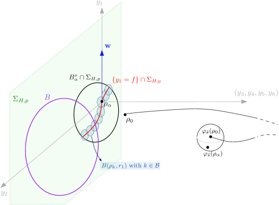
Figure 2. Illustration, when $n=3$, of the covering balls that intersect $B_{\alpha}^{s}$ and loop back for times $\tilde{s}$ near $s$.

Next, we let ${\bf R_{s}}=\frac{r_{\tilde{s}}}{8}$ and use that $\alpha_{2}<\frac{1}{16c^{2}\mathfrak{c}_{0}^{2}}$ to obtain that since $\rho_{0}\in B_{\alpha}^{s}$, for $\rho\in B_{\alpha}^{s}$,

$$d(\rho,\rho_{\alpha})\leq d(\rho_{0},\rho_{\alpha})+d(\rho,\rho_{0})<{r_{0}}+2{\bf R_{s}}<{\frac{r_{\tilde{s}}}{2}}.$$ (2.15)

In particular, (2.15) implies

$$B_{\alpha}^{s}\subset\{\rho\in T^{*}\!M:\;d(\rho,\rho_{\alpha})<{\frac{r_{\tilde{s}}}{2}}\}.$$

Therefore, we have showed that if $\rho\in B_{\alpha}^{s}\cap B(\Sigma_{{}_{\!H,p}},r_{0})$ satisfies (2.14), then $\rho\in\mathcal{U}_{\rho_{\alpha}}^{s}\cap B(\Sigma_{{}_{\!H,p}},r_{0})$ where

$$\mathcal{U}_{\rho_{\alpha}}^{s}=\left\{\rho:\;|y_{1}-f(y_{2},\dots,y_{n-1},0)|<C_{0}e^{\beta|\tilde{s}|}r_{2},\quad d(\rho,\rho_{\alpha})<\tfrac{r_{\tilde{s}}}{2}\right\}.$$

This is illustrated in Figure 2. Next, note that, the number of disjoint tubes in $\{\Lambda_{\rho_{j}}^{\tau}(r_{1})\}_{j=1}^{N}$ that intersect $\mathcal{U}_{\rho_{\alpha}}^{s}\cap B(\Sigma_{{}_{\!H,p}},r_{0})$ is controlled by the number of disjoint balls in the collection $\{B(\rho_{j},r_{1})\}_{j=1}^{N}$ that intersect ${\mathcal{U}}_{\rho_{\alpha}}^{s}\cap\Sigma_{{}_{\!H,p}}$. In addition, for each $j\in\{1,\dots,N\}$ the intersection $B(\rho_{j},r_{1})\cap\Sigma_{{}_{\!H,p}}$ is entirely contained in $\tilde{\mathcal{U}}_{\rho_{\alpha}}^{s}\cap\Sigma_{{}_{\!H,p}}$ where

$$\tilde{\mathcal{U}}_{\rho_{\alpha}}^{s}\!\!=\!\!\left\{\!\rho:|y_{1}-f(y_{2},\dots,y_{n-1},0)|<C_{0}e^{\beta|\tilde{s}|}r_{2}\!+\!4r_{1},\quad\,d(\rho,\rho_{\alpha})<\frac{r_{\tilde{s}}}{2}\!+\!4r_{1}\right\}\!.$$

In particular,

$$\operatorname{vol}(\tilde{\mathcal{U}}_{\rho_{\alpha}}^{s}\cap\Sigma_{{}_{\!H,p}}) \leq(C_{0}e^{\beta|\tilde{s}|}r_{2}+4r_{1})\int_{B(0,\frac{r_{\tilde{s}}}{2}+4r_{1})}\sqrt{1+|\nabla f|^{2}}\,dy_{2}\dots dy_{n-1}.$$

Hence, the number of disjoint balls in the collection $\{B(\rho_{j},r_{1})\}_{j=1}^{N}$ that intersect ${\mathcal{U}}_{\rho_{\alpha}}^{s}\cap\Sigma_{{}_{\!H,p}}$ is controlled by

$${2\sqrt{n-1}\,\mathfrak{c}_{0}c}(C_{0}e^{\beta(|s|+{\tau_{1}})}r_{2}+4r_{1})\,{e^{(\beta+\Lambda)(|s|+{\tau_{1}})}}\big{(}\frac{r_{\tilde{s}}}{2}+4r_{1}\big{)}^{n-2}r_{1}^{-(n-1)}.$$

Here, we used the bound $|\partial_{y_{j}}f|<{\mathfrak{c}_{0}}\,ce^{(\beta+\Lambda)|\tilde{s}|}$ and that $e^{\beta|\tilde{s}|}\leq e^{\beta(|s|+{\tau_{1}})}$.

Finally, note that since $\alpha_{2}<\tfrac{1}{c^{2}\mathfrak{c}_{0}^{2}}$ and $\gamma\geq 3\Lambda+2\beta$, by choosing $\alpha_{1}<1$, we have $r_{1}<\min\{r_{2},r_{\tilde{s}}\}$. Hence, the number of disjoint balls in the collection $\{B(\rho_{j},r_{1})\}_{j=1}^{N}$ that intersect ${\mathcal{U}}_{\rho_{\alpha}}^{s}\cap\Sigma_{{}_{\!H,p}}$ is controlled by ${e^{2\beta{\tau_{1}}}}e^{(2\beta+\Lambda)|s|}r_{2}\tilde{r}_{s}^{n-2}r_{1}^{-(n-1)}$ up to a constant that depends only on $(M,p,k,c,{\mathfrak{I}_{{}_{\!H}}})$. In addition, note that in the collection $\{\Lambda_{\rho_{j}}^{\tau}(r_{1})\}_{j=1}^{N}$ there are ${\mathfrak{D}}$ sets of disjoint tubes of radius $r_{1}$. Therefore, since there are $I_{s}\leq C_{n}R^{n-1}{\bf R_{s}}^{-(n-1)}$ balls $B_{\alpha}^{s}$, for $s=s_{\ell}+t_{j}$ we can build $\mathfrak{b}^{\ell}_{j}$ so that

$$\rho\notin\bigcup_{k\in\mathfrak{b}^{\ell}_{j}}\Lambda_{\rho_{k}}^{\tau}(r_{1})\quad\Longrightarrow\quad d\Big{(}A,\bigcup_{t=s_{\ell}+t_{j}-\frac{{\tau_{1}}}{2}}^{s_{\ell}+t_{j}+\frac{{\tau_{1}}}{2}}\varphi_{t}(\rho)\Big{)}\geq r_{2},$$

and so that for some ${{\bf{C}_{0}}={\bf{C}_{0}}(M,p,k,c,\beta,\mathfrak{I}_{{}_{\!H}})}>0$

$$|\mathfrak{b}^{\ell}_{j}|\leq{{\bf{C}_{0}}}{\mathfrak{D}}\frac{e^{(2\beta+\Lambda)|s|}r_{2}r_{\tilde{s}}^{n-2}R^{n-1}}{r_{1}^{n-1}\mathbf{R}_{s}^{n-1}}.$$

Here, we have used that $e^{2\beta{\tau_{1}}}\leq e^{2\beta}$ since ${\tau_{1}}\leq 1$. Using that $\frac{r_{\tilde{s}}^{n-2}}{\mathbf{R}_{s}^{n-1}}=\frac{8^{n-1}}{r_{\tilde{s}}}$ and adjusting ${{\bf{C}_{0}}}$, we obtain (2.11). This concludes the proofs of the claims in (2.11) and (2.12).

∎

3. Contraction of $\varphi_{t}$ and non-self looping sets

The proofs of Theorems 4 and 6 hinge on controlling how the geodesic flow changes the volume of sets contained in $S\!N^{*}\!H$. As in the previous section, we work with a general Hamiltonian $p$ such that $H$ is conormally transverse for $p$. Let

$$J_{t}:=d\varphi_{t}|_{T_{\rho}\Sigma_{{}_{\!H,p}}}:T_{\rho}\Sigma_{{}_{\!H,p}}\to d\varphi_{t}(T_{\rho}\Sigma_{{}_{\!H,p}}).$$ (3.1)

When the Hamiltonian flow is assumed to be Anosov, we have that for $A_{0}\subset\mathcal{S}_{H}\setminus\mathcal{M}_{H}$, we can split $A_{0}$ into pieces $A_{\pm,0}$ such that there is $C_{0}\geq 1$ satisfying

$$\sup_{\rho\in{A_{\pm,0}}}|\det J_{t}|\leq C_{0}e^{-|t|/C_{{}_{0}}},\qquad\pm t\geq 0.$$ (3.2)

The analysis in this section will be used in Section 5 to prove Theorem 6 and in particular, to handle $\mathcal{S}_{H}\setminus\mathcal{M}_{H}$. This, for instance, is the step which allows us to show that averages over subsets of horospheres have improvements.

Note, however, that the condition in (3.2) is very general and that it may hold in situations where the Hamiltonian flow is not Anosov. For example, such an estimate holds for the geodesic flow at the umbillic points of the triaxial ellipsoid (see e.g. [GT20]). This section is dedicated to study the structure of the set of looping tubes under the assumption that (3.2) holds.

By (2.5), there exists $C_{{}_{\!\varphi}}>0$ depending only on $(M,p)$, so that for all $\Lambda>\Lambda_{\text{max}}$

$$\|d\varphi_{t}\|\leq C_{{}_{\!\varphi}}e^{\Lambda|t|},\qquad t\in{\mathbb{R}}.$$ (3.3)

Let $\mathbf{D}>1$ be so that

$$e^{-\Lambda\mathbf{D}}<\min\Big{\{}\frac{e^{-\Lambda{(1+\tau_{{}_{\!\text{inj}H}})}}}{C_{{}_{\!\varphi}}},\frac{\alpha_{1}}{4},\frac{1}{4}\Big{\}},$$ (3.4)

where $\alpha_{1}=\alpha_{1}(M,p)$ is the constant introduced in Proposition 2.2.

Definition 3.

Let $A_{0}\subset\Sigma_{{}_{\!H,p}}$, $\varepsilon_{0}>0$, $\digamma>0$, $\mathfrak{t}_{0}:[\varepsilon_{0},\infty)\to[1,\infty)$, and $T_{0}>1$ . If the following conditions are satisfied, we say that

$$A_{0}\;\text{ can be}\;{(\varepsilon_{0},\mathfrak{t}_{0},\digamma)\text{-controlled up to time}\;T_{0}.}$$

Let $\varepsilon\geq\varepsilon_{0}$, $\Lambda>\Lambda_{\text{max}}$,

$$0<R_{0}\leq\tfrac{1}{\digamma}e^{-\digamma\Lambda|T_{0}|},\qquad 0<r_{0}<R_{0},$$

and balls $\{B_{0,i}\}_{i=1}^{N}\subset\Sigma_{{}_{\!H,p}}$ centered in $A_{0}$ with radii $\{R_{0,i}\}_{i=1}^{N}\subset[r_{0},R_{0}]$. Then, for $0<\tau<\tfrac{1}{2}\tau_{{}_{\!\text{inj}H}}$ and all

$$A_{1}\subset\bigcup_{i=1}^{N}B_{0,i}\subset A_{0}\qquad\text{and}\qquad 0<r<\tfrac{1}{\digamma}e^{-\digamma\Lambda T_{0}}r_{0},$$

there are balls $\{\tilde{B}_{1,k}\}_{k}\subset\Sigma_{{}_{\!H,p}}$ with radii $\{R_{1,k}\}_{k}\subset[0,{\tfrac{1}{4}R_{0}}]$ so that

1. $\Lambda^{\tau}_{A_{1}\backslash\cup_{k}\tilde{B}_{1,k}}(r)$ is non self-looping for times in $[\mathfrak{t}_{0}(\varepsilon),T_{0}]$,
   

2. $\sum_{k}R_{1,k}^{n-1}\leq\varepsilon\sum_{i}R_{0,i}^{n-1}$,
   

3. ${\inf_{k}}R_{1,k}\geq e^{-\mathbf{D}\Lambda T_{0}}\,{\inf_{i}R_{0,i}}$.

We observe that when we write $A_{1}\backslash\cup_{k}\tilde{B}_{1,k}$ we mean $A_{1}\cap(\Sigma_{{}_{\!H,p}}\backslash\cup_{k}\tilde{B}_{1,k})$.

Note that Definition 3 is vacuous if $T_{0}\leq\mathfrak{t}_{0}(\varepsilon_{0})$.

Lemma 3.1.

There exists $\digamma>0$ depending only on $(M,p,{K_{{}_{\!H}}})$ so that for every monotone decreasing function $f:[0,\infty)\to[0,\infty)$ with $f\in L^{1}([0,\infty))$ and $\Lambda>\Lambda_{\max}$, there exists a function $\mathfrak{t}_{0}:(0,\infty)\to[1,\infty)$ with the following properties.
If $A_{0}\subset\Sigma_{{}_{\!H,p}}$ is so that

$$\sup_{\rho\in{A_{0}}}|\det J_{t}|\leq f(|t|)$$ (3.5)

for all $t\in(0,T_{0})$ or for all $t\in(-T_{0},0)$, then, for all $\varepsilon_{0}>0$,

$$A_{0}\;\text{can be}\;(\varepsilon_{0},\mathfrak{t}_{0},\digamma)\text{-controlled up to time}\;T_{0}$$

in the sense of Definition 3. Furthermore, in addition to conditions (1), (2) and (3) in Definition 3 being satisfied, either

$$\begin{gathered}\bigcup_{t={\mathfrak{t}_{0}(\varepsilon)}}^{T_{0}}\varphi_{t}(\Lambda^{\tau}_{A_{1}\backslash\cup_{k}\tilde{B}_{1,k}}(r))\cap\Lambda_{\Sigma_{{}_{\!H,p}}\backslash\cup_{k}\tilde{B}_{1,k}}^{\tau}(r)=\emptyset,\\ \text{or}\\ {\bigcup_{t=-T_{0}}^{-{\mathfrak{t}_{0}(\varepsilon)}}\varphi_{t}(\Lambda^{\tau}_{A_{1}\backslash\cup_{k}\tilde{B}_{1,k}}(r))\cap\Lambda_{\Sigma_{{}_{\!H,p}}\backslash\cup_{k}\tilde{B}_{1,k}}^{\tau}(r)=\emptyset.}\end{gathered}$$

Note that the last conclusion of Lemma 3.1 differs from condition (1) in Definition 3 since we insist that, after flowing, not only does $\Lambda^{\tau}_{A_{1}\backslash\cup_{k}\tilde{B}_{1,k}}(r)$ not self-intersect (as in (1) of Definition 3, but it does not even intersect $\Sigma_{{}_{\!H,p}}\setminus\cup_{k}\tilde{B}_{1,k}.$

Proof.

We prove the case in which (3.5) holds for all $t\in(0,T_{0})$ (the case in which it holds for all $t\in(-T_{0},0)$ is identical after sending $t\to-t$). Let $\Lambda>\Lambda_{\max}$ and $t_{0}$ be large enough so that $t_{0}>\tau_{{}_{\!\text{inj}H}}+2$ and

$${C_{{}_{\!\varphi}}e^{\Lambda}e^{-\mathbf{D}\Lambda(t_{0}-\tau_{{}_{\!\text{inj}H}}-1)}}\leq 1,$$ (3.6)

where $C_{{}_{\!\varphi}}$ is as in (3.4). We will assume, without loss of generality, that $f(|t|)\geq\frac{1}{C_{\varphi}}e^{-\Lambda t}$. Define

$$\mathfrak{t}_{0}:(0,\infty)\to[1,\infty)\qquad\mathfrak{t}_{0}(\varepsilon)=\inf\Bigg{\{}s\geq t_{0}:\,\,\int_{s}^{\infty}\!\!f(s)ds\leq\frac{\varepsilon\tau_{{}_{\!\text{inj}H}}}{4\alpha}\Bigg{\}},$$

where

$$\alpha:={2^{3n-1}}\gamma^{n-1}\qquad\text{and}\qquad\gamma:=\tfrac{1}{4}C_{\varphi}e^{\Lambda}.$$

Here, $\mathfrak{t}_{0}(\varepsilon)\geq 2$ since $t_{0}>\tau_{{}_{\!\text{inj}H}}+2>2$.

Fix $\varepsilon_{0}>0$ and let $\varepsilon\geq\varepsilon_{0}$. Let $0<\tau<\frac{1}{2}\tau_{{}_{\!\text{inj}H}}$, $R_{0}>0$, $0<r_{0}<R_{0}$ and let $\{B_{0,i}\}_{i=1}^{N}\subset\Sigma_{{}_{\!H,p}}$ be a collection of balls centered in $A_{0}$ with radii $\{R_{0,i}\}_{i=1}^{N}\subset[r_{0},R_{0}]$. Let $A_{1}\subset\bigcup_{i=1}^{N}B_{0,i}$ and $0<r<1$. For each $i\in\{1,\dots,N\}$ let $\{I_{0,i,j}\}_{j=1}^{N_{i}}$ be a collection of disjoint intervals $I_{0,i,j}\subset[{\mathfrak{t}_{0}(\varepsilon)}-2\tau-r,T_{0}+2\tau+r]$ so that $\tfrac{\tau_{{}_{\!\text{inj}H}}}{4}\leq|I_{0,i,j}|<\tfrac{\tau_{{}_{\!\text{inj}H}}}{2}$ and

$$\begin{gathered}\{t\in[{\mathfrak{t}_{0}(\varepsilon)}-2\tau-r,T_{0}+2\tau+r]:\;\varphi_{t}(\Lambda^{0}_{B_{0,i}}(r))\cap\Lambda^{0}_{{}_{\!\Sigma_{{}_{\!H,p}}}}(r)\neq\emptyset\big{\}}\subset\bigcup_{j=1}^{N_{i}}I_{0,i,j},\\ \text{and}\\ {\bigcup_{t\in I_{0,i,j}}\varphi_{t}(\Lambda_{B_{0,i}}^{0}(r){)}\cap\Lambda^{0}_{{}_{\!\Sigma_{{}_{\!H,p}}}}(r)\neq\emptyset.}\end{gathered}$$ (3.7)

For $i\in\{1,\dots,N\}$ and $j\in\{1,\dots,N_{i}\}$ define

$$D_{0,i,j}:=\bigcup_{t\in I_{0,i,j}}\varphi_{t}(\Lambda^{0}_{B_{0,i}}(r))\cap\Lambda^{0}_{{}_{\!\Sigma_{{}_{\!H,p}}}}(r).$$ (3.8)

We claim that for each pair $(i,j)$

$$D_{0,i,j}\subset\bigcup_{\ell=1}^{{L_{i,j}}}\Lambda_{B_{0,i,j,\ell}}^{0}(r)$$ (3.9)

where $\{B_{0,i,j,\ell}\}_{\ell=1}^{{L_{i,j}}}$ are balls centered in $\Sigma_{{}_{\!H,p}}$ with radii $R_{0,i,j,\ell}:=\gamma e^{-\mathbf{D}\Lambda t_{0,i,j}}R_{0,i}$ satisfying

$${L_{i,j}}R_{0,i,j,\ell}^{n-1}\leq\alpha{f(t_{0,i,j})}R_{0,i}^{n-1}$$ (3.10)

(see Figure 3 for an illustration of this covering), where $t_{0,i,j}:=\min\{t:\,t\in I_{0,i,j}\}$. Note that $t_{0,i,j}>1$ for all $(i,j)$ since $r<1$ and ${\mathfrak{t}_{0}(\varepsilon)\geq t_{0}}>\tau_{{}_{\!\text{inj}H}}+2$, and so ${\mathfrak{t}_{0}(\varepsilon)}-2\tau-r>{\mathfrak{t}_{0}(\varepsilon)}-\tau_{{}_{\!\text{inj}H}}-1>1$.

Figure 3. Illustration of a contracting ball and the cover by much smaller balls for the proof of Lemma 3.1.

Note that, since we take $0<r<R_{0}<\digamma^{-1}{e^{-\digamma\Lambda T_{0}}}$, if we let $\digamma_{{}_{\!\!0}}=\digamma_{{}_{\!\!0}}(M,p,K_{{}_{\!H}})$ large enough and assume $\digamma\geq\digamma_{{}_{\!\!0}}$, then $\Sigma_{{}_{\!H,p}}$ is almost flat as a submanifold of $T^{*}\!M$ at scale $R_{0}$. In particular, we have

$$\mathcal{B}(\rho,\tfrac{1}{2}R)\cap\Lambda^{0}_{{}_{\!\Sigma_{{}_{\!H,p}}}}(r)\;\subset\;\Lambda_{B(\rho,R)}^{0}(r),$$

for all $\rho\in\Sigma_{{}_{\!H,p}}$ and $0\leq R\leq R_{0}$. Here we are using $\mathcal{B}$ to denote a ball in $T^{*}\!M$ and $B$ to denote a ball in $\Sigma_{{}_{\!H,p}}$. Therefore, it suffices to show that

$$D_{0,i,j}\subset\bigcup_{\ell=1}^{L_{i,j}}\mathcal{B}_{0,i,j,\ell}.$$ (3.11)

where $\{\mathcal{B}_{0,i,j,\ell}\}_{\ell=1}^{L_{i,j}}\subset T^{*}\!M$ are balls with radii $\mathcal{R}_{0,i,j,\ell}=\tfrac{1}{2}R_{0,i,j,\ell}$ with $R_{0,i,j,\ell}$ as in (3.10).

Let $\rho_{0,i}\in A_{0}$ be the center of $B_{0,i}$ and fix $j\in\{1,\dots,N_{i}\}$. To prove the claim in (3.11) fix $t_{\!{}_{\rho_{0,i}}}\in I_{0,i,j}$ so that $\varphi_{t_{\!{}_{\rho_{0,i}}}}(\rho_{0,i})\in\Lambda^{0}_{\Sigma_{{}_{\!H,p}}}(r)$. Observe that choosing coordinates near $\rho_{0,i}$ and $\varphi_{{}_{{t_{\!{}_{\rho_{0,i}}}}}}(\rho_{0,i})$, we have for $t$ near $t_{\rho_{0,i}}$ and $\rho$ near $\rho_{0,i}$,

$$\varphi_{t}(\rho)=\varphi_{t}(\rho_{0,i})+d\varphi_{t}(\rho-\rho_{0,i})+O(|\rho-\rho_{0,i}|^{2}{e^{2\Lambda|t|}}).$$

If $|\rho-\rho_{0,i}|\leq R_{0,i}$ and $\rho\in\Sigma_{{}_{\!H,p}}$, this gives

$$\varphi_{t}(\rho)=\varphi_{t}(\rho_{0,i})+J_{t}(\rho-\rho_{0,i})+O(R_{{0,i}}^{2}e^{2\Lambda|t|}).$$

Now, let $\{\lambda_{i}(t)\}_{i=1}^{n-1}$ be the singular values of $J_{t}$ ordered so that $\lambda_{i}(t)\leq\lambda_{i+1}(t)$. Then, modulo perturbations controlled by $R_{0}^{2}e^{2\Lambda|t|}$, the set $\varphi_{t}(B_{0,i})$ is an $n-1$ dimensional ellipsoid with axes of length $\lambda_{i}(t)R_{0,i}$. Also, observe that

$$\frac{e^{-\Lambda t}}{C_{{}_{\!\varphi}}}\leq\lambda_{1}(t)\leq\lambda_{n-1}(t)\leq C_{{}_{\!\varphi}}e^{\Lambda t},$$

where $C_{{}_{\!\varphi}}$ is as in (3.3). Since ${\mathfrak{t}_{0}(\varepsilon)}\geq 1$, we note that $e^{-\Lambda{\mathfrak{t}_{0}(\varepsilon)}(\mathbf{D}-1)}<\frac{1}{C_{{}_{\!\varphi}}}$. This ensures that $e^{-\mathbf{D}\Lambda t}<\frac{e^{-\Lambda t}}{C_{{}_{\!\varphi}}}$ for all $t\geq{\mathfrak{t}_{0}(\varepsilon)}$.

Also, note that there exists a constant $\alpha_{{}_{\!M,p}}>0$ so that for all $i\in\{1,\dots,N\}$ and $\rho\in\varphi_{{}_{t_{\rho_{0,i}}}}(\Lambda^{0}_{B_{0,i}}(r))$ we have $d(\rho,\varphi_{t_{\rho_{0,i}}}(B_{0,i}))\leq\alpha_{{}_{\!M,p}}e^{\Lambda t_{\rho_{0,i}}}r$. Define $\digamma$ by

$$\digamma:=\max\{8\alpha_{{}_{\!M,p}}\,,\,{\mathbf{D}+1}\,,\,\digamma_{{}_{\!\!0}}\},$$

and from now on work with $R_{0}\leq\tfrac{1}{\digamma}e^{-\digamma\Lambda|T_{0}|}$. Then, if $0<r<\tfrac{1}{\digamma}e^{-\digamma\Lambda T_{0}}r_{0}$, we have that $r$ is small enough so that $\alpha_{{}_{\!M,p}}e^{\Lambda T_{0}}r\leq\frac{1}{8}e^{-\mathbf{D}\Lambda T_{0}}r_{0}$. In particular, $\alpha_{{}_{\!M,p}}e^{\Lambda t_{\rho_{0,i}}}r<\frac{1}{8}e^{-\mathbf{D}\Lambda t_{0,i,j}}R_{0,i}$ for all $i\in\{1,\dots,N\}$ and there are points $\{q_{\ell}\}_{\ell=1}^{{L_{i,j}}}\subset\varphi_{{}_{t_{\rho_{0,i}}}}(B_{0,i})$ so that

$$\varphi_{{}_{t_{\rho_{0,i}}}}(\Lambda^{0}_{B_{0,i}}(r))\subset\bigcup_{\ell=1}^{{L_{i,j}}}\mathcal{B}(q_{\ell},\tfrac{1}{8}e^{-\mathbf{D}\Lambda t_{0,i,j}}R_{0,i}),$$ (3.12)

where the balls in the right hand side are balls in $T^{*}\!M$. Furthermore,

$$\operatorname{vol}(\varphi_{t_{\rho_{0,i}}}(B_{0,i})) \leq\operatorname{vol}(B_{0,i})(|\det(J_{t_{\rho_{0},i}})|+C_{{}_{\!M,p}}R_{0}^{2}e^{2\Lambda t_{\rho_{0,i}}})$$

$$\leq C_{n}R_{0,i}^{n-1}({f(t_{\rho_{0,i}})}+C_{{}_{\!M,p}}R_{0}^{2}e^{2\Lambda t_{\rho_{0},i}})$$

for some $C_{n}>0$ and $C_{{}_{\!M,p}}>0$. Next, adjust $\digamma$ so that $\digamma^{2}>C_{\varphi}C_{{}_{\!M,p}}$. Then, since $f(|t|)\geq\frac{1}{C_{\varphi}}e^{-\Lambda t}$,

$$\operatorname{vol}(\varphi_{t_{\rho_{0,i}}}(B_{0,i}))\leq{2}C_{n}R_{0,i}^{n-1}{f(t_{\rho_{0,i}})}.$$

Observe that by (3.4) and $t_{\rho_{0,i}}-\frac{\tau_{{}_{\!\text{inj}H}}}{2}\leq t_{0,i,j}\leq t_{\rho_{0,i}}$, we have $e^{-\mathbf{D}\Lambda t_{0,i,j}}<\lambda_{1}(t_{\rho_{0},i})$. Therefore, using that $t_{0,i,j}\leq t_{\rho_{0,i}}$ again, the points $\{q_{\ell}\}_{\ell=1}^{L_{i,j}}$ can be chosen so that

$${L_{i,j}C_{n}({\tfrac{1}{8}}e^{-\mathbf{D}\Lambda t_{0,i,j}}R_{0,i})^{n-1}} \leq 2\operatorname{vol}\Big{(}\varphi_{t_{\rho_{0,i}}}(B_{0,i})\;\bigcap\;\cup_{\ell=1}^{{L_{i,j}}}\mathcal{B}(q_{\ell},{\tfrac{1}{8}}e^{-\mathbf{D}\Lambda t_{0,i,j}}R_{0,i})\Big{)}$$

$$\leq{4}{C_{n}R_{0,i}^{n-1}{f(t_{0,i,j})}}.$$ (3.13)

Note that this yields $L_{i,j}({\tfrac{1}{8}}e^{-\mathbf{D}\Lambda t_{0,i,j}})^{n-1}\leq{4}f(t_{0,i,j})$.

Since $|I_{0,i,j}|<1$, it follows that for every choice of indices $\ell$, $(i,j)$ we have

$$\text{diam}\Big{(}\bigcup_{{t\in I_{0,i,j}}}\varphi_{{}_{t-t_{\rho_{0},i}}}({\mathcal{B}}({q_{\ell},{\tfrac{1}{8}}e^{-\mathbf{D}\Lambda t_{0,i,j}}R_{0,i}))}\cap\Lambda^{0}_{{}_{\!\Sigma_{{}_{\!H,p}}}}(r)\Big{)} \leq{\frac{1}{8}C_{{}_{\!\varphi}}e^{\Lambda}}e^{-\mathbf{D}\Lambda t_{0,i,j}}R_{0,i}{\leq\frac{1}{8}R_{0,i}}$$ (3.14)

where in the last inequality, we use the definition of $\mathbf{D}$. Without loss of generality, we may assume that $C_{{}_{\!\varphi}}\geq 4$ (redefining $\mathbf{D}$ in the process) and hence that $\gamma=\frac{1}{4}C_{{}_{\!\varphi}}e^{\Lambda}\geq 1$ (see (3.10)). This implies that we can find a point $\rho_{0,i,j,\ell}\in\Sigma_{{}_{\!H,p}}$ so that the ball $\mathcal{B}_{0,i,j,\ell}\subset T^{*}\!M$ of center $\rho_{0,i,j,\ell}$ and radius $\mathcal{R}_{0,i,j,\ell}=\tfrac{1}{2}\gamma e^{-\mathbf{D}\Lambda t_{0,i,j}}R_{0,i}=\tfrac{1}{2}R_{0,i,j,\ell}$ contains the set in (3.14) whose diameter is being bounded. Thus, by the definition (3.8) of $D_{0,i,j}$ together with (3.12), we conclude that (3.11) and (3.9) hold. Also, by the definition of $R_{0,i,j,\ell}$, the definition of $\alpha$, and (3), for each choice of $(i,j)$

$$\sum_{\ell=1}^{L_{i,j}}R_{0,i,j,\ell}^{n-1}={L_{i,j}}\gamma^{n-1}(e^{-\mathbf{D}\Lambda t_{0,i,j}}R_{0,i})^{n-1}\leq\alpha{f(t_{0,i,j})}R_{0,i}^{n-1},$$

and hence (3.10) holds. Therefore, from the definition of $\mathfrak{t}_{0}(\varepsilon)$ it follows that

$$\sum_{i,j,\ell}R_{0,i,j,\ell}^{n-1}\leq\alpha\sum_{i,j}{f(t_{0,i,j})}R_{0,i}^{n-1}\leq\frac{4\alpha}{\tau_{{}_{\!\text{inj}H}}}\,{\int_{{\mathfrak{t}_{0}(\varepsilon)}}^{\infty}f(s)ds}\sum_{i}R_{0,i}^{n-1}\leq{\varepsilon\sum_{i}R_{0,i}^{n-1}},$$ (3.15)

where to get the second inequality we used that $t_{0,i,j+1}-t_{0,i,j}\geq\tau_{{}_{\!\text{inj}H}}/4$ implies

$$\sum_{j}\tfrac{\tau_{{}_{\!\text{inj}H}}}{4}{f(t_{0,i,j})}\leq{\int_{{\mathfrak{t}_{0}(\varepsilon)}}^{\infty}f(s)ds}.$$

Let $k=k(i,j,\ell)$ be an index reassignment and write $\tilde{B}_{1,k}=B_{0,i,j,\ell}$ and $R_{1,k}=R_{0,i,j,\ell}$. Note that by the definition of $R_{0,i,j,\ell}$ in (3.10) and the first inequality in (3.6) we know $R_{1,k}\leq\tfrac{1}{4}R_{0}$. In addition, $\cup_{i,j}D_{0,i,j}\subset\cup_{k}\tilde{B}_{1,k}$. According to (3.7) and (3.8) we proved that

$$\bigcup_{t={\mathfrak{t}_{0}(\varepsilon)}-2\tau-r}^{T_{0}+2\tau+r}\varphi_{t}(\Lambda^{0}_{{A_{1}}\backslash\cup_{k}\tilde{B}_{1,k}}(r))\cap\Lambda_{{\Sigma_{{}_{\!H,p}}}\backslash\cup_{k}\tilde{B}_{1,k}}^{0}(r)=\emptyset.$$ (3.16)

We claim that this implies

$$\bigcup_{t={\mathfrak{t}_{0}(\varepsilon)}}^{T_{0}}\varphi_{t}(\Lambda^{\tau}_{{A_{1}}\backslash\cup_{k}\tilde{B}_{1,k}}(r))\cap\Lambda_{{\Sigma_{{}_{\!H,p}}}\backslash\cup_{k}\tilde{B}_{1,k}}^{\tau}(r)=\emptyset.$$ (3.17)

Indeed, if $\rho$ belongs to the set in (3.17), then there exist times $t\in[{\mathfrak{t}_{0}(\varepsilon)}-\tau-r,T_{0}+\tau+r]$, $s\in[-\tau-r,\tau+r]$, and points $q_{0},q_{1}{\in\mathcal{H}_{\Sigma}}$ (see (1.12)) with

$${d(q_{0},A_{1}\backslash\cup_{k}\tilde{B}_{1,k})<r},\qquad{d(q_{1},{\Sigma_{{}_{\!H,p}}}\backslash\cup_{k}\tilde{B}_{1,k})<r}$$

so that $\rho=\varphi_{t}(q_{0})=\varphi_{s}(q_{1})$. Let $\tau^{\prime}\in[-\tau,\tau]$ be so that $|s-\tau^{\prime}|<r$. Then, $\varphi_{-\tau^{\prime}}(\rho)=\varphi_{s-\tau^{\prime}}(q_{1})=\varphi_{t-\tau^{\prime}}(q_{0})$ belongs to the set in (3.16) since $|s-\tau^{\prime}|<r$ and $t-\tau^{\prime}\in[{\mathfrak{t}_{0}(\varepsilon)}-2\tau-r,T_{0}+2\tau+r]$. This means that if the set in (3.16) is empty, then so is the set in (3.17). Finally, (3.17) implies that

$${\Lambda_{A_{1}}^{\tau}(r)}\backslash\bigcup_{k}\Lambda_{\tilde{B}_{1,k}}^{\tau}(r)$$

is non self looping for times in $[{\mathfrak{t}_{0}(\varepsilon)},T_{0}]$. Furthermore, (3.15) now reads

$$\sum_{k}R_{1,k}^{n-1}\leq\varepsilon\sum_{i}R_{0,i}^{n-1}.$$

∎

Lemma 3.2.

Let $E\subset\Sigma_{{}_{\!H,p}}$ be a ball of radius $\delta>0$. Let $\varepsilon_{0}>0$, $\mathfrak{t}_{0}:[\varepsilon_{0},+\infty)\to[1,+\infty)$, $T_{0}>0$, and $\digamma>0$, have the property that $E$ can be $(\varepsilon_{0},{\mathfrak{t}_{0}},\digamma)$-controlled up to time $T_{0}$ in the sense of Definition 3. Let $0<m<\frac{\log T_{0}-\log{\mathfrak{t}_{0}(\varepsilon)}}{\log 2}$ be a positive integer,

$$0\leq R_{0}\leq{\min}\Big{\{}{\tfrac{1}{\digamma}}e^{-{\digamma}\Lambda T_{0}},{\tfrac{\delta}{10}}\Big{\}},\qquad 0<r_{1}<{\tfrac{1}{5\digamma}}e^{-({\digamma}+2\mathbf{D})\Lambda T_{0}}R_{0},$$

and $E_{0}\subset E$ with $d(E_{0},E^{c})>R_{0}$. Let $0<\tau<\tfrac{1}{2}\tau_{{}_{\!\text{inj}H}}$ and suppose that $\Lambda_{{}_{\rho_{j}}}^{\tau}(r_{1})$ is a $({\mathfrak{D}},\tau,r_{1})$ good cover of $\Sigma_{{}_{\!H,p}}$ and set

$$\mathcal{E}:=\{j\in\{1,\dots,{N_{r_{1}}}\}:\Lambda_{\rho_{j}}^{\tau}(r_{1})\cap\Lambda^{\tau}_{E_{0}}(\tfrac{r_{1}}{5})\neq\emptyset\}.$$

Then, there exist $C_{{}_{\!M,p}}>0$ depending only on $(M,p)$ and sets $\{\mathcal{G}_{\ell}\}_{\ell=0}^{m}\subset\{1,\dots N_{r_{1}}\}$, $\mathcal{B}\subset\{1,\dots N_{r_{1}}\}$ so that

$$\mathcal{E}\;\subset\;\mathcal{B}\cup\displaystyle\bigcup_{\ell=0}^{m}\mathcal{G}_{\ell},$$

$$\bullet\;\bigcup_{i\in\mathcal{G}_{\ell}}\Lambda_{\rho_{i}}^{\tau}(r_{1})\text{\; is \;}[\mathfrak{t}_{0},2^{-\ell}T_{0}]\text{\; non-self looping {for every $\ell\in\{0,\dots,m\}$},}$$ (3.18)

$$\bullet\;|\mathcal{G}_{\ell}|\leq C_{{}_{\!M,p}}{\mathfrak{D}}\varepsilon_{0}^{\ell}{\delta^{n-1}}r_{1}^{1-n}\;\;\;{\text{for every}\;\;\ell\in\{0,\dots,m\}},$$ (3.19)

$$\bullet\;|\mathcal{B}|\leq C_{{}_{\!M,p}}{\mathfrak{D}}\varepsilon_{0}^{m+1}{\delta^{n-1}}r_{1}^{1-n}\Big{.}.$$ (3.20)

Proof.

Choose balls $\{B_{0,i}\}_{i=1}^{N}$ centered in $E_{0}$ so that $E_{0}\subset\bigcup_{i=1}^{N}B_{0,i}$ where $B_{0,i}$ has radius $R_{0,i}=R_{0}$ built so that $NR_{0}^{n-1}\leq C_{n}\delta^{n-1}$. This can be done since $R_{0}<\frac{\delta}{10}$. Let $r_{0}:=e^{-{2\mathbf{D}\Lambda T_{0}}}R_{0}$. Since $E$ can be $(\varepsilon_{0},\mathfrak{t}_{0},\digamma)$-controlled up to time $T_{0}$, for

$$0<r<\tfrac{1}{\digamma}e^{-{\digamma}\Lambda T_{0}}r_{0}{=}\tfrac{1}{\digamma}e^{-(\digamma+2\mathbf{D})\Lambda T_{0}}R_{0}$$

there are balls $\{\tilde{B}_{1,k}\}_{k}\subset\Sigma_{{}_{\!H,p}}$ of radii $\{R_{1,k}\}_{k}\subset[0,\tfrac{1}{4}R_{0}]$, so that

$${\inf_{k}}R_{1,k}\geq e^{-\mathbf{D}\Lambda T_{0}}R_{0}\geq r_{0},\qquad\qquad\sum_{k}R_{1,k}^{n-1}\leq\varepsilon_{0}N{R_{0}^{n-1}},\qquad\qquad$$

and with $G_{0}:=\Lambda^{\tau}_{E_{0}\backslash\tilde{E}_{1}}(r)$ non-self-looping for times in $[{\mathfrak{t}_{0}(\varepsilon)},T_{0}],$ where we have set $\tilde{E}_{1}=\cup_{k}\tilde{B}_{1,k}$. Note that we may assume that $E_{0}\cap\tilde{B}_{1,k}\neq\emptyset$ for all $k$. Now, since $R_{1,k}\leq\frac{1}{4}R_{0}$, the ball $\tilde{B}_{1,k}$ is centered at a distance no more than $\frac{1}{4}R_{0}$ from $E_{0}$. So, letting $E_{1}:=\cup_{k}B_{1,k}$ with $B_{1,k}$ the ball of radius $2R_{1,k}$ with the same center as $\tilde{B}_{1,k}$, we have

$$d(E_{1},E^{c})\geq{d(E_{0},E^{c})}-\tfrac{3}{4}R_{0}>(1-\tfrac{3}{4})R_{0}.$$

Next, we set $T_{1}:=2^{-1}T_{0}$ and use that $E_{0}$ can be $(\varepsilon_{0},\mathfrak{t}_{0},\digamma)$-controlled up to time $T_{1}$ (indeed up to time $2T_{1}$). By definition $E_{1}\subset\bigcup_{k}B_{1,k}$ and $R_{0}\leq{\digamma^{-1}}e^{-{\digamma}\Lambda T_{0}}\leq{\digamma^{-1}}e^{-{\digamma}\Lambda T_{1}}$. Therefore, since $0<r<{\digamma^{-1}}e^{-{\digamma}\Lambda T_{0}}r_{0}<{\digamma}^{-1}e^{-{\digamma}\Lambda T_{1}}r_{0}$, there are balls $\{\tilde{B}_{2,k}\}_{k}\subset{\Sigma_{{}_{\!H,p}}}$ of radii $0<R_{2,k}\leq\tfrac{1}{4^{2}}R_{0}$ with

$${\inf_{k}}R_{2,k}\geq e^{-{\mathbf{D}}\Lambda T_{1}}{\inf_{i}}R_{1,i}\qquad\text{and}\qquad\sum_{k}R_{2,k}^{n-1}\leq\varepsilon_{0}\sum_{k}R_{1,k}^{n-1}\leq\varepsilon_{0}^{2}N{R_{0}^{n-1}},$$ (3.21)

so that $G_{1}:=\Lambda^{\tau}_{E_{1}\backslash\tilde{E}_{2}}(r)$ is non-self-looping for times in $[{\mathfrak{t}_{0}(\varepsilon)},T_{1}],$ where we have set $\tilde{E}_{2}=\cup_{k}\tilde{B}_{2,k}$. Since we may assume that $E_{1}\cap\tilde{B}_{2,k}\neq\emptyset$ for all $k$, the balls $\tilde{B}_{2,k}$ are centered at a distance smaller than $\tfrac{1}{4^{2}}R_{0}$ from $E_{1}$. In particular, letting $E_{2}=\cup_{k}B_{2,k}$ where $B_{2,k}$ is the ball of radius $2R_{2,k}$ centered at the same point as $\tilde{R}_{2,k}$, we have

$$d(E_{2},E^{c})\geq d(E_{1},E^{c})-\tfrac{3}{4^{2}}R_{0}>R_{0}\big{(}1-\tfrac{3}{4}-\tfrac{3}{4^{2}}\big{)}.$$

Continuing this way we claim that one can construct a collection of sets $\{G_{\ell}\}_{\ell=1}^{m}\subset\Lambda_{E}^{\tau}(r)$ so that

1. $G_{\ell}$ is non-self-looping for times in $[{\mathfrak{t}_{0}(\varepsilon)},T_{\ell}]$ with $T_{\ell}=2^{-\ell}T_{0}$.

2. There are balls $B_{\ell,k},\tilde{B}_{\ell,k}\subset\Sigma_{{}_{\!H,p}}$ centered at $\rho_{\ell,k}\in{E}$ of radii $2R_{\ell,k}$, $R_{\ell,k}$ respectively so that

   $$G_{\ell}=\Lambda_{E_{\ell}\backslash\tilde{E}_{\ell+1}}^{\tau}(r),$$

   where $E_{\ell}=\bigcup_{k}B_{\ell,k}$ and $\tilde{E}_{\ell}=\bigcup_{k}\tilde{B}_{\ell,k}$.

3. For all $\ell\geq 1$, the radii satisfy $\sup_{\ell}R_{\ell,k}\leq\tfrac{1}{4^{\ell}}R_{0}$,

   $${\inf_{k}}R_{\ell,k}\geq e^{-{2{\mathbf{D}}\Lambda T_{0}}}R_{0}=r_{0}\qquad\text{and}\qquad\sum_{k}R_{\ell,k}^{n-1}\leq\varepsilon_{0}^{\ell}NR_{0}^{n-1}.$$ (3.22)

The claim in (A) follows by construction of $G_{\ell}$. For the claim in (B), we only need to check that the balls $B_{\ell,k}$ are centered in $E$. For this, note that since $R_{\ell,k}\leq\frac{1}{4^{\ell}}R_{0}$, by induction

$$d(E_{\ell},E^{c})>d(E_{\ell-1},E^{c})-\tfrac{3}{4^{\ell}}R_{0}>R_{0}\Big{(}1-{\sum_{j=1}^{\ell}}\tfrac{3}{4^{j}}\Big{)}\geq\frac{1}{{4^{\ell}}}R_{0}.$$

Remark 8.

Note that this actually gives $E_{\ell}\subset E$ and so all of $B_{\ell,k}$ is inside $E$ (not just its center).

We proceed to justify the first inequality in (3.22). Note that the construction yields that $\inf_{k}R_{\ell,k}\geq e^{-{\mathbf{D}}\Lambda T_{\ell}}\inf_{i}R_{\ell-1,i}$ for every $\ell$. Therefore, since $T_{\ell}=2^{-\ell}T_{0}$ and $\inf_{k}R_{\ell,k}\geq e^{-\mathbf{D}\Lambda T_{\ell}}\inf_{i}R_{\ell-1,i}$ (see (3.21)), we obtain

$$\inf_{k}R_{\ell,k}\geq\prod_{{j=0}}^{\ell}e^{-{\mathbf{D}}\Lambda\frac{T_{0}}{{2^{j}}}}R_{0}=e^{-{{\mathbf{D}}\Lambda T_{0}(2-{\frac{1}{2^{\ell}}})}}R_{0}\geq e^{-{2{\mathbf{D}}\Lambda T_{0}}}R_{0}.$$

The construction also yields that $\sum_{k}R_{\ell,k}^{n-1}\leq\varepsilon_{0}\sum_{k}R_{\ell-1,k}^{n-1}$ for all $\ell$. Therefore, the upper bound (3.22) on the sum of the radii follows by induction. Indeed,

$$\sum_{k}R_{\ell,k}^{n-1}\leq\varepsilon_{0}^{\ell}\sum_{k}R_{0,k}^{n-1}=\varepsilon_{0}^{\ell}NR_{0}^{n-1}.$$

Set $r:=5r_{1}$ in the above argument, and define

$$\mathcal{G}_{\ell}:=\{{i\in\mathcal{E}}:\Lambda_{\rho_{i}}^{\tau}(r_{1})\subset G_{\ell}\},\qquad\mathcal{B}:=\mathcal{E}\setminus\bigcup_{{\ell=0}}^{m}\mathcal{G}_{\ell}.$$

Then, since $G_{\ell}$ is $[{\mathfrak{t}_{0}(\varepsilon_{0})},2^{-\ell}T_{0}]$ non-self looping, (3.18) holds. Furthermore, $\mathcal{E}\;\subset\;\mathcal{B}\cup\bigcup_{\ell=0}^{m}\mathcal{G}_{\ell}$ by construction.

We proceed to prove (3.19). Since the cover by tubes can be decomposed into ${\mathfrak{D}}$ sets of disjoint tubes,

$${|\mathcal{G}_{\ell}|\leq{\mathfrak{D}}\frac{\operatorname{vol}(G_{\ell}\cap\Lambda^{\tau}_{E_{0}}(r_{1}))}{\min_{i}\operatorname{vol}(\Lambda_{\rho_{i}}^{\tau}(r_{1}))}}\leq C_{{}_{\!M,p}}{\mathfrak{D}}r_{1}^{1-n}\sum_{k}{R_{\ell,k}^{n-1}}\leq C_{{}_{\!M,p}}{\mathfrak{D}}r_{1}^{1-n}\varepsilon_{0}^{\ell}NR_{0}^{n-1},$$

for some $C_{{}_{\!M,p}}>0$ that depends only on $(M,p)$. Then, (3.19) follows since $NR_{0}^{n-1}\leq C_{n}\delta^{n-1}$.

The rest of the proof is dedicated to obtaining  (3.20). For each $\ell$ note that $E_{\ell}\subset(G_{\ell}\cup\tilde{E}_{\ell+1})$ and $\Lambda_{E_{\ell}}^{\tau}(\frac{r_{1}}{5})\subset\Lambda^{\tau}_{{}_{\!\Sigma_{{}_{\!H,p}}}}(\frac{r_{1}}{5})\subset\cup_{i}\Lambda_{\rho_{i}}^{\tau}(r_{1})$. We claim that for every pair of indices $(\ell,i)$ with $\Lambda_{E_{\ell}}^{\tau}(\frac{r_{1}}{5})\cap\Lambda_{\rho_{i}}^{\tau}(r_{1})\neq\emptyset$, either

$$\Lambda_{\rho_{i}}^{\tau}(r_{1})\subset\Lambda_{{E_{\ell}\setminus\tilde{E}_{\ell+1}}}^{\tau}({5r_{1}})\,\qquad\text{ or }\qquad\Lambda_{\rho_{i}}^{\tau}(r_{1})\cap{\Lambda_{{\tilde{E}_{\ell+1}}}^{\tau}(\tfrac{r_{1}}{5})}\neq\emptyset.$$

Indeed, suppose that $\Lambda_{\rho_{i}}^{\tau}(r_{1})\cap{\Lambda_{{\tilde{E}_{\ell+1}}}^{\tau}(\tfrac{r_{1}}{5})}=\emptyset$. Then, there exists $q\in\mathcal{H}_{\Sigma}\cap\Lambda_{\rho_{i}}^{\tau}(r_{1})$ so that $d(q,\rho_{i})<r_{1}$, $d(q,E_{\ell})<\frac{r_{1}}{5}$, $d(q,\tilde{E}_{\ell+1})\geq\frac{r_{1}}{5}$. In particular, $d(q,E_{\ell}\setminus\tilde{E}_{\ell+1})<\frac{r_{1}}{5}$. Now, suppose that $q_{1}\in\mathcal{H}_{\Sigma}\cap\Lambda_{\rho_{i}}^{\tau}(r_{1})$. Then,

$$d(q_{1},E_{\ell}\setminus\tilde{E}_{\ell+1})\leq d(q_{1},\rho_{i})+d(\rho_{i},q)+d(q,E_{\ell}\setminus{\tilde{E}_{\ell+1}})<\tfrac{11}{5}r_{1}<{5r_{1}}.$$

In particular, $\Lambda_{\rho_{i}}^{\tau}(r_{1})\subset\Lambda_{E_{\ell}\setminus\tilde{E}_{\ell+1}}^{\tau}({5r_{1}})$ as claimed.

Now, suppose that $\Lambda_{\rho_{i}}^{\tau}(r_{1})\cap{\Lambda_{\tilde{E}_{\ell+1}}^{\tau}}(\tfrac{r_{1}}{5})\neq\emptyset$. Then, since $r_{1}<\frac{r_{0}}{5}$ and $R_{\ell,k}\geq r_{0}$, we have

$$\Lambda_{\rho_{i}}^{\tau}(r_{1})\cap\mathcal{H}_{\Sigma}\;\subset E^{\prime}_{\ell+1}$$

where $E^{\prime}_{\ell+1}=\cup_{j}\frac{3}{2}\tilde{B}_{\ell+1,j}$. Observe then that for all $\ell$

$$\Lambda_{E_{\ell}}^{\tau}(\tfrac{r_{1}}{5})\cap\Big{(}\bigcup_{i\in\mathcal{G}_{\ell}}\Lambda_{\rho_{i}}^{\tau}(r_{1})\Big{)}^{c}\;\;\subset\;\;\Lambda_{E^{\prime}_{\ell+1}}^{\tau}(\tfrac{r_{1}}{5}).$$ (3.23)

By induction in $k\geq 2$ we assume that $\Lambda_{E_{0}}^{\tau}(\tfrac{r_{1}}{5})\cap\Big{(}\bigcup_{\ell=0}^{{k}-1}\bigcup_{i\in\mathcal{G}_{\ell}}\Lambda_{\rho_{i}}^{\tau}(r_{1})\Big{)}^{c}\subset\Lambda_{E^{\prime}_{{k}}}^{\tau}(\tfrac{r_{1}}{5}).$ Note that the base case $k=1$ is covered by setting $\ell=0$ in (3.23). Then, using (3.23) with $\ell=k$ together with the inclusion $\tilde{E}_{k}\subset E^{\prime}_{k}\subset E_{k}$ (in fact the balls defining each set have the same center and radii given respectively by $R_{\ell,k}$, $\frac{3}{2}R_{l,k}$ and $2R_{l,k}$) we obtain

$$\Lambda_{E_{0}}^{\tau}(\tfrac{r_{1}}{5})\cap\Big{(}\bigcup_{\ell=0}^{{k}}\bigcup_{i\in\mathcal{G}_{\ell}}\Lambda_{\rho_{i}}^{\tau}(r_{1})\Big{)}^{c}\;\;\subset\;\;\Lambda_{E^{\prime}_{{k}+1}}^{\tau}(\tfrac{r_{1}}{5}).$$

In particular, if $i\in\mathcal{B}$, then ${\Lambda_{E_{0}}^{\tau}(\tfrac{r_{1}}{5})\cap}\Lambda_{\rho_{i}}^{\tau}(r_{1})\subset\Lambda_{{{E}}_{m+1}}^{\tau}({\tfrac{r_{1}}{5}}).$

Therefore,

$$|\mathcal{B}|\leq C_{{}_{\!M,p}}{\mathfrak{D}}r_{1}^{1-n}\sum_{i}{R_{m+1,i}^{n-1}}\leq C_{{}_{\!M,p}}r_{1}^{1-n}\varepsilon_{0}^{m+1}NR_{0}^{n-1},$$

for some $C_{{}_{\!M,p}}$ that depends only on $(M,p)$. This proves (3.20) since $NR_{0}^{n-1}\leq C_{n}\delta^{n-1}$. ∎

4. No Conjugate points: Proof of Theorems 1 and 2

We dedicate this section to the proofs of Theorems 1 and 2. We work with the Hamiltonian $p:T^{*}\!M\to{\mathbb{R}}$ given by $p(x,\xi)=|\xi|_{g(x,\xi)}-1$. The Hamiltonian flow $\varphi_{t}$ associated to it is the geodesic flow, and for any $H\subset M$ we have ${\Sigma_{{}_{\!H,p}}}=S\!N^{*}\!H$.

Let $\Lambda>\Lambda_{\max}$, $t_{0}\in{\mathbb{R}}$, $\varepsilon>0$, and $x\in M$. The study of the behavior of the geodesic flow near $S\!N^{*}\!H$ under the no conjugate points assumption hinges on the fact that if there are no more than $m$ conjugate points (counted with multiplicity) along $\varphi_{t}$ for $t\in(t_{0}-2\varepsilon,t_{0}+2\varepsilon)$, then for every $\rho\in S^{*}_{x}M$ there is a subspace $\mathbf{V_{\!\rho}}\subset T_{\rho}S^{*}_{x}M$ of dimension $n-1-m$ so that for all ${\bf v}\in\mathbf{V_{\!\rho}}$,

$${\|{\bf v}\|}\leq{C\varepsilon^{-{1}}e^{\Lambda|t_{0}|}}\|(d\pi\circ d\varphi_{t})_{\rho}{\bf v}\|,\qquad t\in(t_{0}-\varepsilon,t_{0}+\varepsilon).$$

In particular, this yields that the restriction $(d\pi\circ d\varphi_{t})_{\rho}:\mathbf{V_{\!\rho}}\to T_{\pi\varphi_{t}(\rho)}M$ is invertible onto its image with

$$\|(d\pi\circ d\varphi_{t})_{\rho}^{-1}\|\leq{C\varepsilon^{-{1}}e^{\Lambda|t_{0}|}}.$$ (4.1)

The proof of this result is included in Section 6 as Proposition 6.1 and it holds as long as

$$0<\varepsilon<e^{-C\Lambda|t_{0}|}/C$$ (4.2)

for $C>0$, depending only on $(M,g)$ as defined in as in Proposition 6.1.

In what follows we continue to write $F:T^{*}\!M\to\mathbb{R}^{n+1}$ for the defining function of $S\!N^{*}\!H$ satisfying (2) and we continue to work with

$$\psi:\mathbb{R}\times T^{*}\!M\to\mathbb{R}^{n+1},\qquad\qquad\psi(t,\rho)=F\circ\varphi_{t}(\rho).$$

The following lemma is dedicated to finding a suitable left inverse for $d\psi$.

Lemma 4.1.

Suppose $k>\frac{n+1}{2}$, $\Lambda>\Lambda_{\max}$. There exists $c_{{}_{H}}>0$ depending only on $K_{{}_{H}}$ (as defined in (1.15)) such that the following holds. Let $t_{0}\in{\mathbb{R}}$ and $a>0$ satisfy

$$d(H,\mathcal{C}_{{}_{\!H}}^{2k-n-1,r_{t_{0}},t_{0}})>r_{t_{0}},$$

where $r_{t}=\tfrac{1}{a}e^{-a|t|}$. Then, if $\rho_{0}\in S\!N^{*}\!H$ and

$$d(S\!N^{*}\!H,\varphi_{t_{0}}(\rho_{0}))<\min(r_{t_{0}},{c_{{}_{H}}}),$$

there exists ${\bf w}_{0}\in T_{\rho_{0}}S\!N^{*}\!H$ so that the restriction

$$d\psi_{(t_{0},\rho_{0})}:{\mathbb{R}}\partial_{t}\times\mathbb{R}{\bf w}_{0}\to T_{\psi(t_{0},\rho_{0})}\mathbb{R}^{n+1}$$

has left inverse $L_{(t_{0},\rho_{0})}$ with

$$\|L_{(t_{0},\rho_{0})}\|\leq{C_{{}_{\!M,g}}(1+a)e^{C_{{}_{\!M,g}}(a+\Lambda)|t_{0}|}}$$

where $C_{{}_{\!M,g}}>0$ is a constant depending only on $(M,g)$.

Note that the assumption $k>\frac{n+1}{2}$ is needed for $\mathcal{C}_{{}_{\!H}}^{2k-n-1,r_{t_{0}},t_{0}}$ to be defined. The reason why $2k-n-1$ appears in the exponent of $\mathcal{C}_{{}_{H}}$ is explained in Remark 9.

Proof.

Let $\tilde{F}:=(f_{1},\dots,f_{k})\in C^{\infty}(M;\mathbb{R}^{k})$ be a defining function for $H\subset M$ such that $d\tilde{F}_{y}$ has right inverse ${R}_{{}_{\!\tilde{F},y}}$ with $\|{R}_{{}_{\!\tilde{F},y}}\|\leq 2$ for all $y$ such that $d(y,H)<c_{{}_{H}}$. Note that $c_{{}_{H}}$ can be chosen uniformly depending only on $K_{{}_{H}}$ as in (1.15). Next, define

$$\tilde{\psi}:{\mathbb{R}}\times T^{*}\!M\to{\mathbb{R}}^{k},\qquad\qquad\tilde{\psi}(t,\rho):=\tilde{F}\circ\pi\circ\varphi_{t}(\rho).$$

We claim that there exists ${\bf w}_{0}\in T_{\rho_{0}}S\!N^{*}\!H$ so that

$$d\tilde{\psi}_{(t_{0},\rho_{0})}:\mathbb{R}\partial_{t}\times\mathbb{R}{\bf w}_{0}\to\mathbb{R}^{{k}}$$

is injective and has a left inverse bounded by ${C_{{}_{\!M,g}}(1+a)e^{C_{{}_{\!M,g}}(a+\Lambda)|t_{0}|}}$. Note that this is sufficient as this produces a left inverse for $\psi$ itself.

Observe that for $s\in\mathbb{R}$, $\rho\in S\!N^{*}\!H$, and ${\bf w}\in T_{\rho}S\!N^{*}\!H$,

$$d\tilde{\psi}_{(t,\rho)}(s\partial_{t},{\bf w})=d(\tilde{F}\circ\pi)_{\varphi_{t}(\rho)}\big{(}s\,H_{p}+({d\varphi_{t}})_{\rho}\,{{\bf w}}\big{)}.$$ (4.3)

Note also that since $H$ is conormally transverse for $p$, there exists a neighborhood $W\subset T^{*}\!M$ of $S\!N^{*}\!H$ and $c>0$ so that for $\tilde{\rho}\in W$,

$$\|d(\tilde{F}\circ\pi)_{\varphi_{t}(\tilde{\rho})}H_{p}\|\geq\frac{1}{2}.$$ (4.4)

In particular, the restriction

$$d\tilde{\psi}_{(t_{0},\rho_{0})}:\mathbb{R}\partial_{t}\to\mathbb{R}^{k}$$

has a left inverse bounded by $2$.

We proceed to find ${\bf w}_{0}\in T_{\rho_{0}}S\!N^{*}\!H$ as claimed.

Suppose $d(H,\mathcal{C}_{H}^{2k-n-1,r_{t_{0}},t_{0}})>r_{t_{0}}$. Then, by definition, for all $x\in H$, and every unit speed geodesic $\gamma$ with $\gamma(0)=x$, there the number of conjugate points to $x$ (counted with multiplicity) along $\gamma(t_{0}-r_{t_{0}},t_{0}+r_{t_{0}})$ is smaller than or equal to $m:=2k-n-2$ whenever $d(\gamma(t_{0}),H)<r_{t_{0}}$. In particular, since $d(\varphi_{t_{0}}(\rho_{0}),S\!N^{*}\!H)<r_{t_{0}}$, we have $d(\pi(\varphi_{t_{0}}(\rho_{0})),H)<r_{t_{0}}$. Therefore, by setting $\varepsilon={\min(r_{t_{0}}/2,e^{-C\Lambda|t_{0}|}/C)}$ in (4.1) with $C$ as in (4.2), we have that there is a ${n-1-m}$ dimensional subspace $\mathbf{V}_{\!\rho_{0}}\subset T_{\rho_{0}}S^{*}_{x_{0}}M$ so that $d\pi\circ d\varphi_{t_{0}}|_{\mathbf{V}_{\!\rho_{0}}}$ is invertible onto its image with

$$\|(d\pi\circ d\varphi_{t_{0}}|_{\mathbf{V}_{\!\rho_{0}}})^{-1}\|\leq{C\varepsilon^{-1}e^{\Lambda|t_{0}|}}\leq{C_{{}_{\!M,g}}(1+a)e^{C_{{}_{\!M,g}}(a+\Lambda)|t_{0}|}},$$ (4.5)

for some $C_{{}_{\!M,g}}>0$ depending only on $(M,g)$, and where $x_{0}:=\pi(\rho_{0})$.

Let

$$V=d(\pi\circ\varphi)_{(t_{0},\rho_{0})}\big{(}{\mathbb{R}}\partial_{t}\times(T_{\rho_{0}}(SN_{x_{0}}^{*}H)\cap{\mathbf{V}_{\!\rho_{0}}})\big{)}.$$

Note that since $\dim\mathbf{V}_{\!\rho_{0}}={n-1-m}$, $\dim T_{\rho_{0}}SN_{x_{0}}^{*}H=k-1$, $\dim S^{*}_{x_{0}}M=n-1$, we know that $\dim(T_{\rho_{0}}SN_{x_{0}}^{*}H\cap{\mathbf{V}_{\!\rho_{0}}})\geq{k-1-m}$, and so $\dim V\geq{k-m}$. Also, the restriction

$$d(\pi\circ\varphi)_{(t_{0},\rho_{0})}:\mathbb{R}\partial_{t}\times(T_{\rho_{0}}(SN_{x}^{*}H){\cap\mathbf{V}_{\!\rho_{0}}})\to V$$

is invertible with inverse $\tilde{L}_{(t_{0},\rho_{0})}$ satisfying

$$\|\tilde{L}_{(t_{0},\rho_{0})}\|\leq{C_{{}_{\!M,g}}(1+a)e^{C_{{}_{\!M,g}}(a+\Lambda)|t_{0}|}}.$$

Next, there exists a neighborhood $U\subset M$ of $H$ so that for $y\in U$, $d\tilde{F}_{y}:T_{y}M\to\mathbb{R}^{k}$ is surjective with right inverse $R_{y}$. By assumption, $R_{y}$ is bounded by $2$. Furthermore, we may assume without loss of generality that for $\rho\in T^{*}U\cap W$, $d\pi_{\rho}H_{p}$ lies in the range of $R_{\pi(\rho)}$. Since $\dim(\operatorname{ran}R_{\pi(\varphi_{t_{0}}(\rho_{0}))})=k$, $\dim V\geq{k-m}$, and both $V$ and $\operatorname{ran}R_{\pi(\varphi_{t_{0}}(\rho_{0}))}$ are contained in $T_{\pi(\varphi_{t_{0}}(\rho_{0}))}M$, we know that

$$\dim(\operatorname{ran}R_{\pi(\varphi_{t_{0}}(\rho_{0}))}\cap V)\geq{2k-m-n=2}.$$

Then, this guarantees the existence of ${\bf w}_{0}\in T_{\rho_{0}}(SN_{x_{0}}^{*}H)\cap\mathbf{V}_{\!\rho_{0}}\backslash\{0\}$, so that

$$(d\pi\circ d\varphi_{t_{0}})_{\rho_{0}}{\bf w}_{0}\in\operatorname{ran}R_{\pi(\varphi_{t_{0}}(\rho_{0}))}.$$

Remark 9.

Note that having $\dim(\operatorname{ran}R_{\pi(\varphi_{t_{0}}(\rho_{0}))}\cap V)\geq 1$ would not have been sufficient as $\partial_{t}$ is a component we cannot ignore. It is here where we need that $2k-m-n=2$. In particular, this step explains why the assumption in the lemma is written for the space $\mathcal{C}_{{}_{H}}^{m+1,r_{t_{0}},t_{0}}$ with $m=2k-n-2$.

Then, there exists $\mathbf{x}\in\mathbb{R}^{k}$ so that

$$(d\pi\circ d\varphi_{t_{0}})_{\rho_{0}}{\bf w}_{0}=R_{\pi(\varphi_{t_{0}}(\rho_{0}))}\mathbf{x}.$$

Since $\sup_{y\in U}\|R_{y}\|\leq 2$,

$$\|(d\pi\circ d\varphi_{t_{0}})_{\rho_{0}}{\bf w}_{0}\|\leq 2\|\mathbf{x}\|$$

and by (4.5) we have

$$\|{\bf w}_{0}\|\leq C_{{}_{\!M,g}}ae^{(a+\Lambda)|t_{0}|}\|\mathbf{x}\|.$$

which implies the desired claim since $(d\tilde{F}\circ d\pi\circ d\varphi_{t_{0}})_{\rho_{0}}{\bf w}_{0}=\mathbf{x}$ and so

$$\|d(\tilde{F}\circ\pi)_{\varphi_{t_{0}}(\rho_{0})}((d\varphi_{t_{0}})_{\rho_{0}}{\bf w}_{0})\|\geq(C_{{}_{\!M,g}}a)^{-1}e^{-(a+\Lambda)|t_{0}|}{\|{\bf w}_{0}\|}.$$ (4.6)

Combining (4.4) and (4.6) with (4.3) gives the desired bound on the left inverse for $d\tilde{\psi}$ restricted to $\mathbb{R}\partial_{t}\times\mathbb{R}{\bf w}_{0}$ provided we impose $C_{{}_{\!M,g}}\geq 2$. ∎

Proof of Theorem 2. Let $t_{0}>0$, $a>{\delta_{F}^{-1}}$ so that for $t\geq t_{0}$,

$$d\Big{(}H,\mathcal{C}_{H}^{2k-n-1,r_{t},t}\Big{)}>r_{t},$$ (4.7)

where $r_{t}=\tfrac{1}{a}e^{-at}.$ By Lemma 4.1, for $t\geq t_{0}$, if $\rho\in S\!N^{*}\!H$ and $d(\varphi_{t}(\rho),S\!N^{*}\!H)<{\min(\tfrac{1}{a}e^{-at},c_{{}_{H}})}$, then there exists a ${\bf w}={\bf w}(t,\rho)\in T_{\rho}S\!N^{*}\!H$ so that $d\psi$ restricted to $\mathbb{R}\partial_{t}\times\mathbb{R}{\bf w}$ has left inverse $L_{(t,\rho)}$ with

$$\|L_{(t,\rho)}\|\leq{C_{{}_{\!M,g}}(1+a)e^{C_{{}_{\!M,g}}(a+\Lambda)|t|}},$$

for some $C_{{}_{\!M,g}}>0$ and any $\Lambda>\Lambda_{\max}$. For the purposes of the proof of Theorem 2 fix $\Lambda=2\Lambda_{\max}+1$. Let $c:={(1+a)C_{{}_{\!M,g}}}$, $\beta:={C_{{}_{\!M,g}}(a+\Lambda)}$, and let $t_{1}=t_{1}(a,t_{0})\geq t_{0}$ be so that

$$\|L_{(t,\rho)}\|\leq ce^{\beta|t|}\qquad t\geq t_{1}.$$

In particular, we may cover $S\!N^{*}\!H$ by finitely many balls $\{B_{i}\}_{i=1}^{N}$ of radius $R>0$ (independent of $h$) so that $NR^{n-1}<C_{n}\operatorname{vol}(S\!N^{*}\!H),$ and the hypotheses of Proposition 2.2 hold for each $B_{i}$ choosing $\tilde{c}={a}^{-1}$.

Let $\alpha_{1}=\alpha_{1}(M,g)$ and $\alpha_{2}=\alpha_{2}(M,g,a,\delta_{F})$ be as in Proposition 2.2. Fix $0<\varepsilon<\frac{1}{4}$ and set

$$r_{0}:=h^{2\varepsilon},\qquad r_{1}:=h^{\varepsilon},\qquad r_{2}:=\tfrac{2}{\alpha_{1}}h^{\varepsilon}.$$

Let

$$T_{0}(h)=b\log h^{-1}$$

with $b>0$ to be chosen later. Then, the assumptions in Proposition 2.2 hold provided

$$h^{\varepsilon}<\min\Big{\{}{\tfrac{2}{3\alpha_{1}}}e^{-\Lambda T_{0}}\;,\;\tfrac{\alpha_{1}\alpha_{2}}{2}e^{-\gamma T_{0}},{\tfrac{\alpha_{1}R}{2}}\Big{\}}$$

where $\gamma=\max\{a,3\Lambda+2\beta\}=5\Lambda+2a$. In particular, if we set $\alpha_{3}:=\min\{\tfrac{2}{3\alpha_{1}},\tfrac{\alpha_{1}\alpha_{2}}{2}\}$, the assumptions in Proposition 2.2 hold provided $h<\big{(}\frac{\alpha_{1}R}{2}\big{)}^{\frac{1}{\varepsilon}}$ and

$$T_{0}(h)<\frac{\varepsilon}{\gamma}\log h^{-1}+\frac{\log\alpha_{3}}{\gamma}.$$ (4.8)

We will choose $T_{0}$ satisfying (4.8) later.

Let $0<\tau_{0}<\tau_{{}_{\!\text{inj}H}}$, ${R_{0}=R_{0}(n,k,g,K_{{}_{\!H}})}>0$ be as in Theorem 5. Note that $\tau_{0}=\tau_{0}(M,g,\tau_{{}_{\!\text{inj}H}})$. Also let $h_{0}=h_{0}(M,g)>0$ be the constant given by Theorem 5 and possibly shrink it so that $h_{0}<\big{(}\frac{\alpha_{1}R}{2}\big{)}^{\frac{1}{\varepsilon}}$. Let $\{\rho_{j}\}_{j}\subset S\!N^{*}\!H$ be so that $\{\Lambda^{\tau}_{{}_{\rho_{j}}}(h^{\varepsilon})\}_{j}$ is a $({\mathfrak{D}_{n}},\tau_{0},h^{\varepsilon})$ good cover of $S\!N^{*}\!H$ (existence of such a cover follows from [CG20a, Proposition 3.3] - see Remark 7). Then, for each $i\in\{1,\dots,K\}$ we apply Proposition 2.2 to obtain a cover of $\Lambda_{B_{i}}^{\tau_{0}}(h^{2\varepsilon})$ by tubes $\{\Lambda_{\rho_{{i_{j}}}}^{\tau_{0}}(h^{\varepsilon})\}_{j=1}^{N_{i}}$ with $\rho_{{i_{j}}}\in B_{i}$ and so that $\{1,\dots,N_{i}\}=\mathcal{G}_{i}\cup\mathcal{B}_{i}$,

$$\bigcup_{j\in\mathcal{G}_{i}}\Lambda_{\rho_{j}}^{\tau_{0}}(h^{\varepsilon})\quad\text{is }\;\;[t_{0},T_{0}(h)]\;\;\text{ non-self looping,}$$

$$h^{\varepsilon(n-1)}|\mathcal{B}_{i}|\leq{\bf{C}_{0}}\tfrac{2}{\alpha_{1}}\;h^{\varepsilon}\;R^{n-1}\;T_{0}{e^{4({\Lambda+\beta})T_{0}}},$$

where ${\bf{C}}_{0}={\bf{C}}_{0}(M,g,k,a)>0$. We choose $b>0$ so that $b<\frac{\varepsilon}{12({\Lambda+\beta})}$ and (4.8) is satisfied for all $h<h_{0}$. Note that this implies that $b=b(M,g,a,\delta_{F})$. In particular, there exists $h_{0}=h_{0}(\tau_{0},{\bf{C}}_{0})$, so that for all $0<h<h_{0}$,

$$h^{\varepsilon(n-1)}|\mathcal{B}_{i}|<h^{\frac{\varepsilon}{3}}R^{n-1}.$$ (4.9)

We next apply Theorem 5 $\delta:=2\varepsilon$, and $R(h):=h^{\varepsilon}$ (not to be confused with $R$). If needed, we shrink $h_{0}$ so that $5h^{2\varepsilon}\leq R(h)<R_{0}$ for all $0<h<h_{0}$. We let $\alpha<1-2\varepsilon$ and let $b$ be small enough so that $T_{0}(h)\leq 2\alpha T_{e}(h)$ for all $0<h<h_{0}$. We also let $\mathcal{B}=\cup_{i=1}^{K}\mathcal{B}_{i}$, and work with only one set of good indices $\mathcal{G}:=\mathcal{I}_{h}(w)\backslash\mathcal{B}$. We choose $t_{\ell}(h)=t_{1}$ and $T_{\ell}(h)=T_{0}(h)$. Note that (4.9) gives

$$R(h)^{\frac{n-1}{2}}|\mathcal{B}|^{\frac{1}{2}}\leq h^{\frac{\varepsilon}{6}}(KR^{n-1})^{\frac{1}{2}}\leq h^{\frac{\varepsilon}{6}}{{C_{n}}^{\!\frac{1}{2}}}\operatorname{vol}(S\!N^{*}\!H)^{\frac{1}{2}}.$$

Since in addition

$$|\mathcal{G}|\leq|\mathcal{I}_{h}(w)|\leq K(\max_{1\leq i\leq K}N_{i})\leq\operatorname{vol}(S\!N^{*}\!H)C_{n}{h^{-\varepsilon(n-1)}},$$

Let $N>0$. Theorem 5 yields the existence of constants $C_{n,k}>0$, $\tilde{C}=\tilde{C}({M,g,\tau_{0},\varepsilon})>0$ and $C_{{}_{\!N}}>0$ so that for all $0<h<h_{0}$

$$h^{\frac{k-1}{2}}\Big{|}\int_{H}wu\,d\sigma_{H}\Big{|}$$

$$\leq\frac{C_{n,k}{\operatorname{vol}(S\!N^{*}\!H)^{\frac{1}{2}}}\|w\|_{{}_{\!\infty}}C_{{}_{n}}^{\tfrac{1}{2}}}{\tau_{0}^{\frac{1}{2}}}\!\Bigg{(}\Bigg{[}h^{\frac{\varepsilon}{6}}+\frac{t_{1}^{\frac{1}{2}}}{T_{0}^{\frac{1}{2}}(h)}\Bigg{]}\!\!\|u\|_{{{}_{\!L^{2}(M)}}}\!+\frac{T_{0}^{\frac{1}{2}}(h)t_{1}^{\frac{1}{2}}}{h}\|(-h^{2}\Delta_{g}-I)u\|_{{}_{{H_{\operatorname{scl}}^{-2}(M)}}}\Bigg{)}$$

$$+\frac{\tilde{C}}{h}{\|w\|_{\infty}}\|(-h^{2}\Delta_{g}-I)u\|_{\text{\raisebox{5.69046pt}{${{}_{\!H_{\operatorname{scl}}^{\frac{k-3}{2}}\!\!(M)}}$}}}\!+C_{{}_{\!N}}h^{N}\big{(}\|u\|_{{{}_{\!L^{2}(M)}}}\!+{\|(-h^{2}\Delta_{g}-I)u\|_{{\text{\raisebox{5.69046pt}{${{}_{\!H_{\operatorname{scl}}^{\frac{k-3}{2}}\!\!(M)}}$}}}}}\big{)}$$ (4.10)

$$\leq C{\|w\|_{{}_{\!\infty}}}\left(\frac{\|u\|_{{{}_{\!L^{2}(M)}}}}{\sqrt{\log h^{-1}}}+\frac{\sqrt{\log h^{-1}}}{h}\|(-h^{2}\Delta_{g}-I)u\|_{\text{\raisebox{5.69046pt}{${{}_{\!H_{\operatorname{scl}}^{\frac{k-3}{2}}\!\!(M)}}$}}}\right)$$ (4.11)

where $C=C(M,g,k,t_{0},a,\delta_{F},\operatorname{vol}(S\!N^{*}\!H),\tau_{{}_{\!\text{inj}H}})>0$ is some positive constant and $h_{0}=h_{0}(\delta,M,g,\tau_{0},k,a,w,R_{0})$ is chosen small enough so that the last term on the right of (4.10) can be absorbed. Note that the $\varepsilon$ dependence of $C$ and $h_{0}$ is resolved by fixing any $\varepsilon<\tfrac{1}{4}$. ∎

Proof of Theorem 1. Note that if $H=\{x\}$ then $S\!N^{*}\!H=S_{x}^{*}M$ and $\operatorname{vol}(S^{*}_{x}M)=c_{n}$ for some $c_{n}>0$ that depends only on $n$. Next, note that $\tau_{{}_{\!\text{inj}H}}(\{x\})$ and $\delta_{F}$ can be chosen uniform on $M$ and that $H_{p}r_{H}=2$. Moreover, in this case, $w=1$ and $K_{{}_{\!H}}$ can be taken arbitrarily small so $R_{0}=R_{0}(n,k,p,K_{{}_{\!H}})$ can be taken to be uniform on $M$.

Therefore, since the constant in (4.11) and $h_{0}$ depends only on

$$M,\;g,\;k,\;t_{0},\;a,\;\delta_{F},\;\operatorname{vol}(S\!N^{*}\!H),\;\tau_{{}_{\!\text{inj}H}},$$

all of the terms on the right hand side of (4.11) are uniform for $x\in M$ completing the proof of Theorem 1. ∎

5. No focal points or Anosov geodesic flow: Proof of Theorems 4 and 6

Next we analyze the cases in which $(M,g)$ has no focal points or Anosov geodesic flow. For $\rho\in S\!N^{*}\!H$ we continue to write $N_{\pm}(\rho)=T_{\rho}(S\!N^{*}\!H)\cap E_{\pm}(\rho)$ and define the functions $m,m_{\pm}:S\!N^{*}\!H\to\{0,\dots,n-1\}$

$$\begin{gathered}m(\rho):=\dim(N_{+}(\rho)+N_{-}(\rho)),\qquad m_{\pm}(\rho):=\dim N_{\pm}(\rho),\end{gathered}$$ (5.1)

and note that the continuity of $E_{\pm}(\rho)$ implies that $m,\,m_{\pm}$ are upper semicontinuous (see e.g. [CG19, Lemma 20]). We will need extensions of $N_{\pm}(\rho)$, $m_{\pm}(\rho)$ to neighborhoods of $S\!N^{*}\!H$ for our next lemma. To have this, for each $\rho$ in a neighborhood of $S\!N^{*}\!H$ define the set

$$\mathcal{F}_{\!\rho}:=\{q\in T^{*}\!M:\;F(q)=F(\rho)\},$$

where $F$ is the defining function for $S\!N^{*}\!H$ introduced in (2). Since for $\rho\in S\!N^{*}\!H$, $\mathcal{F}_{\!\rho}=S\!N^{*}\!H$, $\mathcal{F}_{\!\rho}$ can be thought of as a family of ‘translates’ of $S\!N^{*}\!H$. We then define

$$\tilde{N}_{\pm}(\rho):=T_{\rho}\mathcal{F}_{\!\rho}\cap E_{\pm}(\rho)\qquad\text{and}\qquad\tilde{m}_{\pm}(\rho):=\dim\tilde{N}_{\pm}(\rho).$$

Note that since $T_{\rho}\mathcal{F}_{\!\rho}$ is smooth in $\rho$ and agrees with $T_{\rho}(S\!N^{*}\!H)$ for $\rho\in S\!N^{*}\!H$, $\tilde{m}_{\pm}(\rho)$ is upper semicontinuous with $\tilde{m}_{\pm}|_{S\!N^{*}\!H}=m_{\pm}.$ In what follows we continue to write $\mathcal{S}_{H}=\{\rho\in S\!N^{*}\!H:\;\,T_{\rho}(S\!N^{*}\!H)=N_{-}(\rho)+N_{+}(\rho)\}$.

The following lemma shows that if $\rho\in S\!N^{*}\!H$ does not belong to $\mathcal{S}_{H}$ and $\varphi_{t}(\rho)$ is close enough to $\rho$ for $t$ sufficiently large, then $(d\varphi_{t})_{\rho}{\bf w}$ leaves ${T_{{\varphi_{t}(\rho)}}}\mathcal{F}_{\!{\varphi_{t}}(\rho)}$ for some ${\bf w}\in T_{\rho}S\!N^{*}\!H$.

Lemma 5.1.

Suppose $(M,g)$ has Anosov geodesic flow or no focal points and let $K\subset(S\!N^{*}\!H\backslash{\mathcal{S}_{H}})$ be a compact set. Then there exist positive constants $c_{{}_{\!K}},t_{{}_{\!K}},\delta_{{}_{\!K}}>0$ so that if ${d(\rho,K)\leq\delta_{{}_{\!K}}}$, $|t|\geq t_{{}_{\!K}}$, and

$${\varphi_{t}}(\rho)\in\;\overline{B(\rho,\delta_{{}_{\!K}})},$$

then there is $\mathbf{w}=\mathbf{w}(t,\rho)\in T_{\rho}(S\!N^{*}\!H){\setminus\{0\}}$ with

$$\inf\{\|d{\varphi_{t}}(\mathbf{w})+{\bf v}\|:\;{\bf v}\in T_{\varphi_{t}(\rho)}\mathcal{F}_{\!{\varphi_{t}}(\rho)}{+}{\mathbb{R}}H_{p}\}\geq c_{{}_{\!K}}\|\mathbf{w}\|.$$ (5.2)

Proof.

First note that since $\tilde{m}_{\pm}$ are upper semi-continuous, $K$ is compact, and $K\cap\mathcal{S}_{H}$ is empty, there exists $\delta_{{}_{\!\tilde{K}}}>0$ so that $d(K,\mathcal{S}_{H})>\delta_{{}_{\!\tilde{K}}}.$ Therefore, to prove the lemma we work with the compact set $\tilde{K}:=\{\rho\in S\!N^{*}\!H:\;d(\rho,K)\leq\frac{\delta_{{}_{\!\tilde{K}}}}{2}\}$ and insist that $\delta_{K}<\frac{\delta_{{}_{\!\tilde{K}}}}{2}$.

Let $\rho\in\tilde{K}$. Since $T_{\rho}(S\!N^{*}\!H)\neq N_{+}(\rho)+N_{-}(\rho)$, we may choose ${\bf u}={\bf u}(\rho)$ such that

$${\bf u}\in T_{\rho}(S\!N^{*}\!H)\setminus(N_{+}(\rho)+N_{-}(\rho)),\qquad\|{\bf u}\|=1.$$

Now, let $\mathbf{u}_{+}\in E_{+}(\rho)$ and $\mathbf{u}_{-}\in E_{-}(\rho)$ be so that

$$\mathbf{u}=\mathbf{u}_{+}+\mathbf{u}_{-}.$$

In particular, ${\bf u}_{\pm}\notin N_{\pm}(\rho)$.

When studying the case $t>t_{K}$, we will use that ${\bf u}_{-}$ grows along the positive time flow, while for $t<-t_{K}$ we will use that ${\bf u}_{+}$ grows along the negative time flow. Since the arguments are identical, except with time reversed and the roles of ${\bf u}_{+}$ and ${\bf u}_{-}$ switched, we only explicitly write that for $t>t_{K}$.

We claim that there is $C_{{}_{\!K}}>0$ such that for all $\rho\in\tilde{K}$, we may in addition choose ${\bf u}={\bf u}(\rho)$ such that

$$\begin{gathered}{\bf u}_{-}\in E_{-}(\rho)\cap(N_{-}(\rho))^{\perp}\cap(E_{+}(\rho)\cap E_{-}(\rho))^{\perp},\\ C_{{}_{\!K}}^{-1}\|{\bf u}_{+}\|\leq\|{\bf u}_{-}\|\leq C_{{}_{\!K}}\|{\bf u}_{+}\|.\end{gathered}$$ (5.3)

For this, we set

$$\begin{gathered}\bar{N}_{\pm}(\rho):=N_{\pm}(\rho)\cap\Big{(}E_{+}(\rho)\cap E_{-}(\rho)\Big{)}^{\perp},\\ U_{\pm}(\rho):=E_{\pm}(\rho)\cap(N_{\pm}(\rho))^{\perp}\cap\Big{(}E_{+}(\rho)\cap E_{-}(\rho)\Big{)}^{\perp}.\end{gathered}$$

We then observe that

$$(\mathbb{R}H_{p}(\rho))^{\perp}=U_{+}(\rho)\oplus\bar{N}_{+}(\rho)\oplus\Big{(}E_{+}(\rho)\cap E_{-}(\rho)\Big{)}\oplus\bar{N}_{-}(\rho)\oplus U_{-}(\rho)$$

and decompose a vector ${\bf v}\in(\mathbb{R}H_{p})^{\perp}$ correspondingly as

$${\bf v}={\bf v}_{U_{+}}+{\bf v}_{\bar{N}_{+}}+{\bf v}_{0}+{\bf v}_{\bar{N}_{-}}+{\bf v}_{U_{-}}.$$

Suppose the claim in (5.3) fails. Then, for all $n\in\mathbb{N}$, there are $\rho_{n}\in\tilde{K}$ such that for all ${\bf v}\in T_{\rho_{n}}S\!N^{*}\!H$,

$$n^{-1}\|{\bf v}_{U_{+}}+{\bf v}_{\bar{N}_{+}}+{\bf{v}}_{0}\|>\|{\bf v}_{U_{-}}+{\bf v}_{\bar{N}_{-}}\|,\qquad\text{ or }\qquad n\|{\bf v}_{U_{+}}+{\bf v}_{\bar{N}_{+}}+{\bf{v}_{0}}\|<\|{\bf v}_{U_{-}}+{\bf v}_{\bar{N}_{-}}\|.$$

In particular, since ${\bf v}_{\bar{N}_{-}}\in T_{\rho_{n}}S\!N^{*}\!H$, we have ${\bf{v}}-{\bf{v}}_{\bar{N}_{-}}\in T_{\rho_{n}}S\!N^{*}\!H$, and hence, for all ${\bf v}\in T_{\rho_{n}}S\!N^{*}\!H$,

$$n^{-1}\|{\bf v}_{U_{+}}+{\bf v}_{\bar{N}_{+}}+{\bf{v}}_{0}\|>\|{\bf v}_{U_{-}}\|,\qquad\text{ or }\qquad n\|{{\bf v}_{U_{+}}}+{\bf v}_{\bar{N}_{+}}+{\bf{v}_{0}}\|<\|{\bf v}_{U_{-}}\|.$$

Since $\tilde{K}$ is compact, we may assume $\rho_{n}\to\rho\in\tilde{K}$. Then, for all ${\bf v}\in T_{\rho}S\!N^{*}\!H$, there are ${\bf v}_{n}\in T_{\rho_{n}}S\!N^{*}\!H$ such that ${\bf v}_{n}\to{\bf v}$. Let ${\bf v}\in T_{\rho}S\!N^{*}\!H\setminus(N_{+}(\rho)+N_{-}(\rho))$ and ${\bf v}_{n}\to{\bf v}$ as above.

Then,

$$n^{-1}\|{\bf v}_{n,U_{+}}+{\bf v}_{n,\bar{N}_{+}}+{\bf{v}}_{n,0}\|>\|{\bf v}_{n,U_{-}}\|,\qquad\text{ or }\qquad n\|{\bf v}_{U_{+}}+{\bf v}_{n,\bar{N}_{+}}+{\bf{v}}_{n,0}\|<\|{\bf v}_{n,U_{-}}\|.$$

Extracting a subsequence again, we may assume that one of these inequalities holds for all $n$. We consider first the case

$$n^{-1}\|{\bf v}_{n,U_{+}}+{\bf v}_{n,\bar{N}_{+}}+{\bf{v}}_{n,0}\|>\|{\bf v}_{n,U_{-}}\|.$$

Now, since ${\bf v}_{n}\to{\bf v}$, and $E_{+}(\rho)$ is continuous,

$${\bf v}_{n,U_{+}}+{\bf v}_{n,\bar{N}_{+}}+{\bf{v}}_{n,0}\to\tilde{\bf v}_{+}\in E_{+}(\rho)$$

In particular, this implies that ${\bf v}_{n,U_{-}}\to 0$ and hence ${\bf v}_{n,\bar{N}_{-}}\to{\bf v}-\tilde{\bf v}_{+}.$ Using that $\rho\mapsto T_{\rho}S\!N^{*}\!H$ and $\rho\mapsto E_{-}(\rho)$ are continuous maps, and that ${\bf v}_{n,\bar{N}_{-}}\in E_{-}(\rho_{n})\cap T_{\rho_{n}}S\!N^{*}\!H$, we have ${\bf v}-\tilde{\bf v}_{+}\in N_{-}(\rho)$ and hence also ${\bf v}_{+}\in N_{+}(\rho)$. Therefore, ${\bf v}\in N_{+}(\rho)+N_{-}(\rho)$, a contradiction.

Next, we consider the other case:

$$n\|{\bf v}_{U_{+}}+{\bf v}_{n,\bar{N}_{+}}+{\bf{v}}_{n,0}\|<\|{\bf v}_{n,U_{-}}\|.$$

Then, since ${\bf v}_{n}\to{\bf v}$, ${\bf v}_{n,U_{-}}$ is bounded and hence ${\bf v}_{U_{+}}+{\bf v}_{n,\bar{N}_{+}}+{\bf{v}}_{n,0}\to 0$. In particular, ${\bf v}_{n,U_{-}}+{\bf v}_{n,\bar{N}_{-}}\to{\bf v}$, so ${\bf v}\in E_{-}(\rho)$ and hence ${\bf v}\in N_{-}(\rho)$, a contradiction. Since both cases lead to a contradiction, we have proved the claim (5.3).

Since $d\varphi_{t}:E_{-}(\rho)\to E_{-}(\varphi_{t}(\rho))$ and $d\varphi_{t}:E_{+}(\rho)\cap E_{-}(\rho)\to E_{+}(\varphi_{t}(\rho))\cap E_{-}(\varphi_{t}(\rho))$ are isomorphisms, we have

$$\dim\operatorname{span}\begin{pmatrix}d\varphi_{t}(\mathbf{u}_{-}),&d\varphi_{t}(N_{-}(\rho))\end{pmatrix}=1+\dim N_{-}(\rho).$$

Also, note that since $\tilde{m}_{-}$ is upper semicontinuous and integer valued, we may choose $\delta>0$ uniform in $\rho\in S\!N^{*}\!H$ so that $\dim\tilde{N}_{-}(q)\leq\dim N_{-}(\rho)$ for all $q\in B(\rho,\delta)$. For any $t$ and $q\in B(\rho,\delta)$ we then have

$$\dim\operatorname{span}\begin{pmatrix}d\varphi_{t}(\mathbf{u}_{-}),&d\varphi_{t}(N_{-}(\rho))\end{pmatrix}\geq 1+\dim{\tilde{N}_{-}(q)}.\vskip 6.0pt plus 2.0pt minus 2.0pt$$ (5.4)

Next, note that $\operatorname{span}\!\begin{pmatrix}d\varphi_{t}(\mathbf{u}_{-}),&d\varphi_{t}(N_{-}(\rho))\end{pmatrix}\subset E_{-}(\varphi_{t}(\rho))$. Suppose now that $\varphi_{t}(\rho)\in B(\rho,\delta)$ for some $t$ and note that if $d\varphi_{t}({\bf w})\in E_{-}(\varphi_{t}(\rho))\backslash\tilde{N}_{-}(\varphi_{t}(\rho))$, then $d\varphi_{t}({\bf w})\notin T_{\varphi_{t}(\rho)}\mathcal{F}_{\!\varphi_{t}(\rho)}$. In particular, relation (5.4) gives that there exists a linear combination

$${\bf w_{t}}=a_{t}\,\mathbf{u}_{-}+{\bf e}_{-}(t)\;{\in E_{-}(\rho)},$$

with ${\bf e}_{-}(t)\in N_{-}(\rho)$, so that $d\varphi_{t}{\bf w_{t}}\in(\tilde{N}_{-}(\varphi_{t}(\rho)))^{\perp}$ with $\|d\varphi_{t}{\bf w_{t}}\|=1$. If we had that ${\bf w_{t}}$ was a tangent vector in $T_{\rho}(S\!N^{*}\!H)$ and we had control on $\|{\bf w}_{t}\|$ we would be done proving (5.2). Note that to say this we are using that $d\varphi_{t}{\bf w}_{t}\in E_{-}(\varphi_{t}(\rho))$ and that $E_{-}(\varphi_{t}(\rho)){\perp}\mathbb{R}H_{p}$. However, since $\mathbf{u}_{-}$ is not in $T_{\rho}S\!N^{*}\!H$ we have to modify ${\bf w_{t}}$. Consider the vector

$${\bf\tilde{w}_{t}}=a_{t}\,\mathbf{u}+{\bf e}_{-}(t),$$

and note that ${\bf\tilde{w}_{t}}\in T_{\rho}(S\!N^{*}\!H)$ and

$$d\varphi_{t}({\bf\tilde{w}_{t}})=d\varphi_{t}({\bf w_{t}})+a_{t}\,d\varphi_{t}(\mathbf{u}_{+}).$$

Let $\delta_{1}>0$ be so that $1-\delta_{1}\tilde{\mathbf{B}}{C_{{}_{\!K}}}>\frac{1}{2}$. We claim that there is $t_{{}_{\!K}}>0$, depending only on $(M,p,K)$, so that for $t>t_{{}_{\!K}}$,

$$\|{\bf w_{t}}\|\leq{\delta_{1}}\qquad\text{and}\qquad|a_{t}|<\delta_{1}{\|\mathbf{u}_{-}\|^{-1}}.$$ (5.5)

Note that this yields that for $t$ large enough, $d\varphi_{t}({\bf\tilde{w}_{t}})$ approaches $d\varphi_{t}({\bf w_{t}})\notin T_{\varphi_{t}(\rho)}\mathcal{F}_{\!{\varphi_{t}}(\rho)}$. In particular, the $t$-flowout of the ${\bf\tilde{w}_{t}}$ direction in $T_{\rho}(S\!N^{*}\!H)$ approaches $E_{-}(\varphi_{t}(\rho))$ (see Figure 4). We postpone the proof of (5.5) until the end, and show how to finish the proof assuming it holds.

Figure 4. Schematic of the rotation of $\bf\tilde{w}_{t}$ under the geodesic flow.

We next observe that there exists $\tilde{\mathbf{B}}>0$ so that if ${\bf w}\in E_{\pm}(\rho)$ then $\|d\varphi_{t}{\bf w}\|\leq\tilde{\mathbf{B}}\|{\bf w}\|$ as $t\to\pm\infty$. Indeed, in the Anosov case $\tilde{\mathbf{B}}=\mathbf{B}$, where $\mathbf{B}$ is defined in (1.20), and in the no focal point case the existence of $\tilde{\mathbf{B}}$ is guaranteed by [Ebe73a, Proposition 2.13, Corollary 2.14]. We can therefore conclude from (5.3) and (5.5) that

$$\|\pi_{t,\rho}(d\varphi_{t}{\bf\tilde{w}_{t}})\|\geq\|\pi_{t,\rho}(d\varphi_{t}{\bf w_{t}})\|-\|a_{t}\,\pi_{t,\rho}(d\varphi_{t}{\bf u}_{+})\|>1-\delta_{1}\tilde{\mathbf{B}}{C_{{}_{\!K}}},$$

and

$$\|\mathbf{\tilde{w}_{t}}\|=\|{\bf w}_{t}+a_{t}{\bf u}_{+}\|\leq\|\mathbf{w}_{t}\|+|a_{t}|\|\mathbf{u}_{+}\|\leq\delta_{1}(1+C_{{}_{\!K}}),$$

where $\pi_{t,\rho}$ denotes orthogonal projection onto $E_{-}(\varphi_{t}(\rho))\cap(\tilde{N}_{-}(\varphi_{t}(\rho)))^{\perp}.$ In particular,

$$\|\pi_{t,\rho}(d\varphi_{t}{\bf\tilde{w}_{t}})\|\geq\frac{1-\delta_{1}\tilde{\mathbf{B}}{C_{{}_{\!K}}}}{\delta_{1}(1+C_{{}_{\!K}})}\|\mathbf{\tilde{w}_{t}}\|.$$

Therefore, there exist positive constants $c_{{}_{\!K}}$, $\delta_{{}_{\!K}}$ and $t_{{}_{\!K}}$ (uniform for $\rho\in K$) so that if ${\varphi_{t}}(\rho)\in B(\rho,\delta_{{}_{\!K}})$ for some $t$ with $|t|>t_{{}_{\!K}}$, then there is $\mathbf{w}=\tilde{\mathbf{w}}_{t}\in T_{\rho}(S\!N^{*}\!H)$ so that

$$\|d{\varphi_{t}}(\mathbf{w})+\mathbb{R}H_{p}+T_{{\varphi_{t}}(\rho)}\mathcal{F}_{\!{\varphi_{t}}(\rho)}\|\geq c_{{}_{\!K}}\|\mathbf{w}\|.$$ (5.6)

This would finish the proof assuming that the claim in (5.5) holds.

We proceed to prove (5.5). We start with the Anosov case. By the definition of Anosov geodesic flow,

$$\|(d\varphi_{t}|_{E_{-}})^{-1}\|\leq\mathbf{B}e^{-t/\mathbf{B}},\quad t\geq 0.$$

Thus, since ${\bf w_{t}}\in E_{-}(\rho)$ and $\left\|d\varphi_{t}{\bf w_{t}}\right\|=1$, we find $\|{\bf w_{t}}\|\leq\mathbf{B}e^{-t/\mathbf{B}}$. In particular, since $\mathbf{u}_{-}$ and ${\bf e}_{-}(t)$ are orthogonal, we have

$$|a_{t}|\leq\mathbf{B}e^{-t/\mathbf{B}}\|\mathbf{u}_{-}\|^{-1},\qquad{t\geq 0}.$$

This proves the claim (5.5) in the Anosov flow case after choosing $t_{{}_{\!K}}>0$ large enough so that $\mathbf{B}e^{-t/\mathbf{B}}\leq\delta_{1}$.

We next consider the non-focal points case. Define $\mathcal{C}_{+}^{\alpha}(\rho)\subset T_{\rho}(S^{*}\!M)$ to be the conic set of vectors forming an angle larger than or equal to $\alpha>0$ with $E_{+}(\rho)$. Let $\alpha_{{}_{\!K}}>0$ be so that ${\mathbf{w}_{t}}\in E_{-}(\rho)\cap\mathcal{C}_{+}^{\alpha_{{}_{\!K}}}(\rho)$ for all $\rho\in\tilde{K}$. By [Ebe73a, Proposition 2.6] $(d\pi)_{\rho}:E_{\pm}(\rho)\oplus H_{p}(\rho)\to T_{\pi(\rho)}M$ is an isomorphism for each $\rho$. In particular, letting $V(\rho)\subset T_{\rho}(S^{*}\!M)$ denote the vertical vectors, we have that $E_{\pm}(\rho)\cap V(\rho)=\emptyset$ and $V(\rho)\oplus E_{+}(\rho)\oplus H_{p}(\rho)=T_{\pi(\rho)}S^{*}M$. In addition, since $(M,g)$ has no focal points, $\cup_{\rho\in S^{*}M}E_{\pm}(\rho)$ is closed [Ebe73a, see right before Proposition 2.7] and hence there exists $c_{{}_{\alpha_{{}_{\!K}}}}>0$ depending only on $\alpha_{{}_{\!K}}$ so that

$$\mathbf{w}_{t}={\bf e_{+}}+{\bf v}$$

with

$$c_{{}_{\alpha_{{}_{\!K}}}}\|{\bf e_{+}}\|\leq\|\mathbf{w}_{t}\|\leq\frac{1}{c_{{}_{\alpha_{{}_{\!K}}}}}\|{\bf v}\|.$$

and ${\bf e_{+}}\in E_{+}(\rho)$, ${\bf v}\in{V}(\rho)$. By [Ebe73a, Remark 2.10], for all $R>0$ there exists $T(R)>0$ so that $\|Y(t)\|\geq R\|Y^{\prime}(0)\|$ for all $t>T(R)$, where $Y(t)$ is any Jacobi field with $Y(0)=0$ and perpendicular to a unit speed geodesic $\gamma$ with $\gamma(0)\in\tilde{K}$. Since ${\bf v}$ is a vertical vector, we may consider $Y(t)=d\pi\circ d\varphi_{t}({\bf v})$, and this implies that $Y^{\prime}(0)=\bf{K}{\bf v}^{\sharp}$ (see Appendix 6 for an explanation of the connection map $\bf{K}$, and the $\sharp$ operator). We therefore have that $\|d\varphi_{t}{\bf v}\|\geq R\|{\bf v}\|$ for all $t>T(R)$. In particular, then

$$\|d\varphi_{t}\mathbf{w}_{t}\|=\|d\varphi_{t}\mathbf{v}+d\varphi_{t}\mathbf{e}_{+}\|\geq R\|{\bf v}\|-\tilde{\mathbf{B}}\|{\bf e_{+}}\|\geq(Rc_{{}_{\alpha_{{}_{\!K}}}}-c_{{}_{\alpha_{{}_{\!K}}}}^{-1}\tilde{\mathbf{B}})\|\mathbf{w}_{t}\|.$$

So, choosing $R(\alpha_{{}_{\!K}})=c_{{}_{\alpha_{{}_{\!K}}}}^{-1}(\delta_{1}^{-1}+c_{{}_{\alpha_{{}_{\!K}}}}^{-1}\tilde{\mathbf{B}})$, we have that for $t\geq t_{{}_{\!K}}:=T(R(\alpha_{{}_{\!K}}))$,

$$1=\|d\varphi_{t}\mathbf{w}_{t}\|\geq\delta_{1}^{-1}\|\mathbf{w}_{t}\|.$$

In particular, for $t\geq t_{{}_{\!K}}$, since $\mathbf{u}_{-}$ is orthogonal to ${\bf e_{-}}(t)$, we obtain $1=\|d\varphi_{t}\mathbf{w}_{t}\|\geq\delta_{1}^{-1}\|\mathbf{w}_{t}\|\geq\delta_{1}^{-1}|a_{t}|{\|\mathbf{u}_{-}\|},$ completing the proof of the lemma in the case of manifolds without focal points.
∎

When $(M,g)$ has Anosov geodesic flow, we need to define a notion of angle between a vector and $E_{\pm}(\rho)$. Let $\pi_{\pm}:T_{\rho}S^{*}\!M\to E_{\pm}(\rho)$ be the projection onto $E_{\pm}(\rho)$ along $E_{\mp}(\rho)\oplus H_{p}(\rho)$ i.e. if ${\bf{u}}={\bf{v}}_{+}+{\bf{v}}_{-}+rH_{p}$ with $r\in\mathbb{R}$, ${\bf{v}}_{\pm}\in E_{\pm}(\rho)$, then $\pi_{\pm}({\bf{u}})={\bf{v}}_{\pm}$. For $\rho\in S^{*}\!M$, define ${\Theta}^{\pm}_{\rho}:{(\mathbb{R}H_{p}(\rho))^{\perp}}\setminus\{0\}\to[0,\infty]$ by

$${{\Theta}^{\pm}_{\rho}}(\mathbf{u}):=\frac{\|\pi_{\mp}\mathbf{u}\|}{\|\pi_{\pm}\mathbf{u}\|}.$$ (5.7)

Note that ${\Theta}^{\pm}_{\rho}$ should be thought of as measuring the tangent of the angle from $E_{\pm}(\rho)$, and that given a compact subset $K$ of $T^{*}\!M\backslash\{0\}$ there exists $C_{{}_{\!K}}>0$ so that for all $\rho\in K$, $t\in\mathbb{R}$, and $\mathbf{u}\in T_{\rho}S^{*}\!M$, we have

$$\frac{e^{\pm t/C_{{}_{\!K}}}}{C_{{}_{\!K}}}\,{\Theta}^{\pm}_{\rho}(\mathbf{u})\leq{\Theta}^{\pm}_{\rho}(d\varphi_{t}\mathbf{u})\leq C_{{}_{\!K}}e^{\pm C_{{}_{\!K}}t}\,{\Theta}^{\pm}_{\rho}(\mathbf{u}).$$ (5.8)

In what follows we will use the fact that by [CG20a, Proposition 3.3] there are $\mathfrak{D}_{n}>0$ depending only on $n$, $\tau_{{}_{\!S\!N^{*}\!H}}>0$ depending only on $\tau_{{}_{\!\operatorname{inj}H}}$, and ${R_{0}>0}$ depending only on $(n,k,K_{H})$ and finitely many derivatives of the curvature and second fundamental form of $H$, so that for ${0<}\tau<\tau_{{}_{\!S\!N^{*}\!H}}$ and ${0<}r<R_{0}$, there is a $({\mathfrak{D}}_{n},\tau,r)$ good cover of $S\!N^{*}\!H$.

Lemma 5.2.

Let $(M,g)$ have Anosov geodesic flow and $H\subset M$ satisfy $\mathcal{A}_{H}=\emptyset$. Then, there exist $c=c(M,g,H)>0$, $C=C(M,g,H)>2$, ${I}>0$, $t_{0}>1$, so that for all $\Lambda>\Lambda_{\text{max}}$ the following holds.

Let $T_{0}\geq t_{0}$,  $m=\big{\lfloor}\frac{\log T_{0}-\log t_{0}}{\log 2}\big{\rfloor}$,   $0<\tau_{0}<\tau_{{}_{\!S\!N^{*}\!H}}$,  $0<\tau\leq\tau_{0}$,

$$0\leq r_{1}\leq\min\{e^{-CT_{0}},{R_{0}}\},$$

and $\{\Lambda_{\rho_{j}}^{\tau}(r_{1})\}_{j=1}^{N_{r_{1}}}$ be a $({\mathfrak{D}_{n}},\tau,r_{1})$ good cover of $S\!N^{*}\!H$. Then, for each $i\in\{1,\dots,{I}\}$ there are sets of indices $\{\mathcal{G}_{i,\ell}\}_{\ell=0}^{m}\subset\{1,\dots,N_{r_{1}}\}$ and $\mathcal{B}\subset\{1,\dots,N_{r_{1}}\}$ so that

$$\bigcup_{i=1}^{{I}}\bigcup_{\ell=0}^{m}\mathcal{G}_{i,\ell}\cup\mathcal{B}=\{1,\dots,N_{r_{1}}\},$$

and for every $i\in\{1,\dots,{{I}}\}$ and every $\ell\in\{0,\dots,m\}$

• $\bigcup_{j\in\mathcal{G}_{i,\ell}}\Lambda_{\rho_{j}}^{\tau}(r_{1})$ is $[t_{0},2^{-\ell}T_{0}]$ non-self looping,
  

• $|\mathcal{G}_{i,\ell}|\leq c\,5^{-\ell}\,r_{1}^{1-n},$
  

• $|\mathcal{B}|\leq c\,{\Big{(}\frac{t_{0}}{T_{0}}\Big{)}^{\frac{\log 5}{\log 2}}}\,r_{1}^{1-n}.$

We note that if $H_{0}\subset M$ is an embedded submanifold, there exists a neighborhood $U$ of $H_{0}$ (in the $C^{\infty}$ topology) so that the constants $c=c(M,p,H)$ and $C=C(M,p,H)$ in Lemma 5.2 are uniform for $H\in U$.

Proof.

Let $0\leq r_{0}\leq\tfrac{1}{C}e^{-\Lambda T_{0}}r_{1}$. Then $\{\Lambda_{\rho_{j}}^{\tau}(r_{1})\}_{j=1}^{N_{r_{1}}}$ covers $\Lambda_{{}_{\!S\!N^{*}\!H}}^{\tau}(r_{0})$ since $r_{0}\leq\tfrac{1}{2}r_{1}$. Throughout this proof we will repeatedly use that if $F:T^{*}\!M\to\mathbb{R}^{n+1}$ is the defining function for $S\!N^{*}\!H$, then there exist $\delta_{0},c_{0}>0$ so that for $q\in T^{*}\!M$

$$d(q,S\!N^{*}\!H)\leq\delta_{0}\quad\Longrightarrow\quad\|dF{\bf v}\|\geq c_{0}\inf\big{\{}\|{\bf v}+{\bf u}\|:\;{\bf u}\in T_{q}\mathcal{F}_{q}\big{\}}\quad\forall{\bf v}\in T_{q}(T^{*}\!M).$$ (5.9)

In addition, let $\nu>0$ be so that $\rho\mapsto E_{\pm}(\rho)\in C^{\nu}$ and define $c_{{}_{\!H}}>0$ so that

$$\sup_{{q_{1},q_{2}}\in S\!N^{*}\!H}\Big{(}\|\tan^{-1}\circ\Theta^{{\pm}}_{{q_{1}}}\|_{L^{\infty}(T_{{q_{1}}}S\!N^{*}\!H)}-\|\tan^{-1}\circ\Theta^{{\pm}}_{{q_{2}}}\|_{L^{\infty}(T_{{q_{2}}}S\!N^{*}\!H)}\Big{)}\leq\frac{1}{c_{{}_{\!H}}}{d(q_{1},q_{2})^{\nu}}.$$ (5.10)

This implies that that for all $\varepsilon>0$, there exists $\delta_{\varepsilon}>0$ so that for every ball $\tilde{B}\subset S\!N^{*}\!H$ of radius $\delta_{\varepsilon}$ we have that

$$\sup_{\rho_{1},\rho_{2}\in\tilde{B}}\;\Big{|}\|\tan^{-1}{\Theta}^{\pm}_{\rho_{1}}\|_{L^{\infty}(T_{\rho_{1}}S\!N^{*}\!H)}-\|\tan^{-1}{\Theta}^{\pm}_{\rho_{2}}\|_{L^{\infty}(T_{\rho_{2}}S\!N^{*}\!H)}\Big{|}<\varepsilon.$$ (5.11)

Also, since $\mathcal{A}_{H}=\emptyset$, we know that for every $\rho\in\mathcal{S}_{H}$ we must have that either $m_{+}(\rho)=0$ or $m_{-}(\rho)=0$, where we continue to write $m_{{\pm}}(\rho)=\dim N_{\pm}(\rho)$. Therefore, choosing

$$\varepsilon=\varepsilon(M,p,H)<1$$ (5.12)

small enough, depending only on $(M,g,H)$, and shrinking $\delta_{\varepsilon}$ if necessary, we may also assume that if $\tilde{B}\cap\mathcal{S}_{H}\neq\emptyset$ then either

$$m_{-}(\rho) =0\;\;\text{and}\;\;{\Theta}^{+}_{\rho}\leq\varepsilon\;\;\;\text{for all}\;\;\rho\in\tilde{B},$$

or (5.13)

$$m_{+}(\rho) =0\;\;\text{and}\;\;{\Theta}^{-}_{\rho}\leq\varepsilon\;\;\;\text{for all}\;\;\rho\in\tilde{B}.$$

Furthermore, we assume that $\delta_{\varepsilon}\leq\tfrac{2}{9}\big{[}\varepsilon c_{{}_{\!H}}\big{]}^{\frac{1}{\nu}}$.

Next, let $\{B_{i}\}_{i=1}^{N_{\varepsilon}}\subset S\!N^{*}\!H$ be a cover of $S\!N^{*}\!H$ with

$$S\!N^{*}\!H\subset\bigcup_{i=1}^{N_{\varepsilon}}B_{i},\qquad\qquad B_{i}\;\;\text{ball of radius}\;\tfrac{1}{2}\delta_{\varepsilon}.$$

Let $\mathcal{I}_{\mathcal{S}_{H}}:=\{i\in\{1,\dots,N_{\varepsilon}\}:\;B_{i}\cap\mathcal{S}_{H}\neq\emptyset\}$, and define $K=K_{\varepsilon}$ by

$$K:=\bigcup_{i\in\mathcal{I}_{\mathcal{S}_{H}}}(S\!N^{*}\!H\backslash{B_{i}}).$$

Since $K\subset(S\!N^{*}\!H\backslash\mathcal{S}_{H})$ is compact and the geodesic flow is Anosov, by Lemma 5.1 there exist positive constants $c_{{}_{\!K}},t_{{}_{\!K}},\delta_{{}_{\!K}}$ so that $d(K,\mathcal{S}_{H})>\delta_{{}_{\!K}}$ and, if $d(\rho,K)\leq\delta_{{}_{\!K}}$ and $\varphi_{t}(\rho)\in\overline{B(\rho,\delta_{{}_{\!K}})}$ for some $|t|>t_{{}_{\!K}}$, then there exists ${\bf w}={\bf w}(t,\rho)\in T_{\rho}(S\!N^{*}\!H)$ so that

$$\inf\{\|d\varphi_{t}(\mathbf{{\bf w}})+{\bf v}\|:\;{\bf v}\in{T_{\varphi_{t}(\rho)}}\mathcal{F}_{\!\varphi_{t}(\rho)}+{\mathbb{R}}H_{p}\}\geq c_{{}_{\!K}}\|\mathbf{{\bf w}}\|.$$ (5.14)

We then introduce a cover $\{D_{i}\}_{i\in I_{K}}\subset S\!N^{*}\!H$ of $K$ by balls with

$$K\subset\bigcup_{i\in I_{K}}D_{i},\qquad\qquad D_{i}\;\;\text{ball of radius}\;{\tfrac{1}{4}R,}$$

where

$$R:=\min\{\delta_{{}_{\!K}},\delta_{0},\tfrac{1}{2}\delta_{\varepsilon},{\delta_{F}}\}$$

and $\delta_{F}$ is as in (2). Note that $R$ depends only on $(M,p,H,K)$. It follows that,

$$S\!N^{*}\!H\subset\left(\bigcup_{i\in\mathcal{I}_{\mathcal{S}_{H}}}B_{i}\;\;\cup\;\;\bigcup_{i\in\mathcal{I}_{K}}D_{i}\right)$$ (5.15)

where each ball $B_{i}$ satisfies (5.11) and (5.13), and each ball $D_{i}$ satisfies (5.14). Also,

$$\mathcal{S}_{H}\cap D_{i}=\emptyset\;\;\;\forall i\in\mathcal{I}_{K}\qquad\text{and}\qquad\mathcal{S}_{H}\cap B_{i}\neq\emptyset\;\;\;\forall i\in\mathcal{I}_{\mathcal{S}_{H}}.$$

Since $S\!N^{*}\!H$ can be split as in (5.15), we present how to treat $D_{i}$ with $i\in\mathcal{S}_{H}$ and $B_{i}$ with $i\in\mathcal{I}_{K}$ separately.

Treatment of $D\in\{D_{i}\}_{i\in\mathcal{I}_{K}}$.

Let $D\in\{D_{i}\}_{i\in\mathcal{I}_{K}}$. Note that since $R\leq\min\{\delta_{{}_{\!K}},\delta_{0}\}$, by (5.14) we know that if $\rho\in D$ and $|t|\geq t_{{}_{\!K}}$ are so that $d(\varphi_{t}(\rho),\rho)<R$, then there exists ${\bf w}={\bf w}(t,\rho)\in T_{\rho}(S\!N^{*}\!H)$ so that for all $s\in{\mathbb{R}}$

$$\|dF(d\varphi_{t}{\bf w}+sH_{p})\| \geq c_{0}\inf\big{\{}\|d\varphi_{t}{\bf w}+sH_{p}+{\bf u}\|:\;{\bf u}\in T_{\varphi_{t}(\rho)}\mathcal{F}_{\varphi_{t}(\rho)}\big{\}}$$

$$\geq c_{0}\inf\big{\{}\|d\varphi_{t}{\bf w}+{\bf v}\|:\;{\bf v}\in T_{\varphi_{t}(\rho)}\mathcal{F}_{\varphi_{t}(\rho)}+{\mathbb{R}}H_{p}\big{\}}$$

$$\geq c_{0}c_{{}_{\!K}}\|{\bf w}\|,$$

where we used (5.9) to get the first inequality and (5.14) for the third one. This implies that if $|t|\geq t_{{}_{\!K}}$ and $\rho\in D$ are so that $d(\varphi_{t}(\rho),\rho)<R$, then $d\psi(t,\rho):=d(F\circ\varphi_{t})(t,\rho)$ has a left inverse $L_{(t,\rho)}$ when restricted to ${\mathbb{R}}\partial_{t}\oplus{\mathbb{R}}{\bf w}$ with $\|L_{(t,\rho)}\|\leq(c_{0}c_{{}_{\!K}})^{-1}$.

Let $\alpha_{1},\alpha_{2}$ be as in Proposition 2.2, and note that they only depend on $(M,g,H,{K})$. We aim to apply this proposition with $A=D$, $B=D$, $\beta=0$, $c={(c_{0}c_{{}_{\!K}})^{-1}}$, $a=0$, $\tilde{c}=\frac{R}{4}$. Let $t_{1}$ satisfy

$$t_{1}\geq\max\{1,t_{{}_{\!K}}\}.$$ (5.16)

Note that $t_{1}$ depends only on $(M,p,H,{K})$.

Next, let $T_{0}\geq t_{1}$. By construction, if $(t,\rho)\in[t_{1},T_{0}]\times D$ are so that $d(\varphi_{t}(\rho),D)\leq\tilde{c}$, by (5.16) we have

$$d(\varphi_{t}(\rho),\rho)\leq d(\varphi_{t}(\rho),D)+\operatorname{diam}(D)\leq\tilde{c}+2(\tfrac{1}{4}R)<R.$$

In this case there exists ${\bf w}={\bf w}(t,\rho)\in T_{\rho}(S\!N^{*}\!H)$ so that $d\psi(t,\rho)$ has a left inverse $L_{(t,\rho)}$ when restricted to ${\mathbb{R}}\partial_{t}\oplus{\mathbb{R}}{\bf w}$ with $\|L_{(t,\rho)}\|\leq c_{0}c_{{}_{\!K}}\leq c$.

Let $C>0$ be so that

$$\frac{1}{C}<{\min}\{\tfrac{1}{2},\tfrac{1}{3\alpha_{1}}\}\qquad\text{and}\qquad e^{-CT_{0}}\leq\min\{\tfrac{1}{8}\alpha_{1}R,\;\tfrac{1}{2}\alpha_{1}\alpha_{2}e^{-{3\Lambda}T_{0}}\}.$$ (5.17)

Set $r_{2}:=\frac{2}{\alpha_{1}}r_{1}$ and note that by construction, and the assumptions on the pair $(r_{0},r_{1})$, we have

$$r_{1}<\alpha_{1}\,r_{2},\qquad r_{2}\leq\min\{{\tfrac{1}{4}R},\alpha_{2}\,e^{-{3\Lambda}T_{0}}\},\qquad r_{0}<\tfrac{1}{3}\,e^{-\Lambda T_{0}}r_{2}.$$

Also, note that we work with $0<\tau<\tau_{0}<\tau_{{}_{\!S\!N^{*}\!H}}$, and that by definition $\tau_{{}_{\!S\!N^{*}\!H}}<\tfrac{1}{2}\tau_{{}_{\!\text{inj}H}}$ as requested by Proposition 2.2. We apply Proposition 2.2 to the cover $\{\Lambda_{\rho_{j}}^{\tau}(r_{1})\}_{j\in\mathcal{E}_{{}_{\!D}}}$ of $\Lambda_{{}_{\!D}}^{\tau}(r_{0})$ where

$$\mathcal{E}_{{}_{\!D}}:=\{j:\Lambda_{\rho_{j}}^{\tau}(r_{1})\cap\Lambda_{{}_{\!{D}}}^{\tau}(r_{0})\neq\emptyset\}.$$ (5.18)

Then, there is a partition $\mathcal{E}_{{}_{\!D}}=\mathcal{G}_{{}_{\!D}}\cup\mathcal{B}_{{}_{\!D}}$ with

$$|\mathcal{B}_{{}_{\!D}}|\leq{\bf{C}_{0}}\;\frac{{R}^{n-1}}{{r_{1}^{n-2}}}\;T_{0}e^{{4\Lambda}T_{0}},$$ (5.19)

where ${\bf{C}_{0}}={\bf{C}_{0}}(M,g,k,c_{0},c_{{}_{K}})>0$, and so that

$$\bigcup_{j\in\mathcal{G}_{{}_{\!D}}}\Lambda^{\tau}_{\rho_{j}}(r_{1})\qquad\text{is}\;\;\;[t_{1},T_{0}]\text{ non-self looping}.$$ (5.20)

Treatment of $B\in\{B_{i}\}_{i\in\mathcal{I}_{\mathcal{S}_{H}}}$

Let $B\in\{B_{i}\}_{i\in\mathcal{I}_{\mathcal{S}_{H}}}$. Since (5.13) is satisfied for all $\rho\in B$, we shall focus on the case where $m_{-}(\rho)=0$ for all $\rho\in B$; the other being similar after sending $t\mapsto-t$ in the arguments below.

Suppose $B$ is the ball $B(\rho_{{}_{\!B}},\tfrac{1}{2}\delta_{\varepsilon})$ for some $\rho_{{}_{\!B}}\in S\!N^{*}\!H$ and let

$$E:=B(\rho_{{}_{\!B}},\tfrac{3}{4}\delta_{\varepsilon})\subset S\!N^{*}\!H,\qquad\tilde{B}:=B(\rho_{{}_{\!B}},\delta_{\varepsilon})\subset S\!N^{*}\!H.$$

Note that $B\subset E\subset\tilde{B}$, and that ${\Theta}^{+}_{\rho}\leq\varepsilon$ for all $\rho\in\tilde{B}$ by (5.13).

We claim that there exist a function $\mathfrak{t}_{2}:[\tfrac{1}{5},+\infty)\to[1,+\infty)$ that depends only on $(M,p)$, and a constant $\digamma>0$ depending on $(M,p,K_{{}_{\!H}})$, so that

$$E\;\;\text{can be}\;\;(\tfrac{1}{5},\mathfrak{t}_{2},\digamma)\text{-controlled up to time}\;T_{0}.$$ (5.21)

If the claim in (5.21) holds, setting $R_{0}:=\min\{{\tfrac{1}{\digamma}}e^{-{\digamma}\Lambda T_{0}},\tfrac{1}{8}\delta_{\varepsilon}\}$ and noting that $d(B,E^{c})=\tfrac{1}{4}\delta_{\varepsilon}>R_{0}$, we may apply Lemma 3.2 to the ball $E$ with $E_{0}=B$ and $\varepsilon_{0}=\tfrac{1}{5}$. Indeed, by possibly enlarging $C>0$ in (5.17) so that

$$e^{-CT_{0}}<\tfrac{1}{5\digamma}e^{-({\digamma}+2\mathbf{D})\Lambda T_{0}}R_{0},$$ (5.22)

by the assumption that $r_{1}\leq e^{-CT_{0}}$ we conclude $0<r_{1}<{\tfrac{1}{5\digamma}}e^{-({\digamma}+2\mathbf{D})\Lambda T_{0}}R_{0}$. Therefore, letting

$$\mathcal{E}_{{}_{\!B}}:=\{j:\Lambda_{\rho_{j}}^{\tau}(r_{1})\cap\Lambda_{{}_{\!B}}^{\tau}(r_{0})\neq\emptyset\},$$ (5.23)

there exists $C_{{}_{M,g}}>0$ depending only on $(M,g)$, so that for every integer $0<m<\frac{\log T_{0}-\log t_{0}(\frac{1}{5})}{\log 2}$ there are sets $\{\mathcal{G}_{{}_{\!B,\ell}}\}_{\ell=0}^{m}\subset\{1,\dots N_{r_{1}}\}$, $\mathcal{B}_{{}_{\!B}}\subset\{1,\dots N_{r_{1}}\}$ satisfying

$$\mathcal{E}_{{}_{\!B}}\subset\mathcal{B}_{{}_{\!B}}\cup\displaystyle\bigcup_{\ell=0}^{m}\mathcal{G}_{{}_{\!B,\ell}},\qquad\bigcup_{i\in\mathcal{G}_{{}_{\!B,\ell}}}\Lambda_{\rho_{i}}^{\tau}(r_{1})\text{ is }[t_{2}(\tfrac{1}{5}),2^{-\ell}T_{0}]\text{ non-self looping}$$

$$|\mathcal{G}_{{}_{\!B,\ell}}|\leq C_{{}_{M,p}}\frac{\delta_{\varepsilon}^{n-1}}{5^{\ell}}\frac{1}{r_{1}^{n-1}},\qquad\text{ and }\qquad|\mathcal{B}_{{}_{\!B}}|\leq C_{{}_{M,p}}\frac{\delta_{\varepsilon}^{n-1}}{5^{m+1}}\frac{1}{r_{1}^{n-1}},$$ (5.24)

for all $\ell\in\{0,\dots,m\}$. We shall use this construction later in the proof, namely below the “Constructing the complete cover” title, to build the complete cover.

We dedicate the rest of the argument to proving the claim in (5.21). Let $\digamma>0$ satisfy

$$\frac{1}{\digamma}<\min\Big{\{}\frac{\alpha}{4},\frac{\alpha^{2}}{4},\frac{\alpha\,}{{60\bf{C}_{0}}},\frac{[\varepsilon c_{{}_{\!\!H}}]^{\frac{1}{\nu}}}{3},{\frac{\varepsilon^{{\frac{1}{\nu}}}}{C^{{\frac{1}{\nu}}}_{{}_{\!\Theta}}}},\frac{1}{11},{\frac{\nu}{2}}\Big{\}},$$ (5.25)

where $\alpha:=\min\{{\frac{1}{3}},\alpha_{1},\alpha_{2}\}$, $c_{{}_{\!\!H}}$ is defined in (5.10), ${\bf{C}_{0}}$ is the positive constant introduced in Proposition 2.2 (that depends only on $(M,g,H,\varepsilon)$ when the left inverse is bounded by ${{\frac{2C_{\varphi}}{c_{0}\,\varepsilon}}}$), and $C_{{}_{\!\Theta}}$ is so that for all $\rho_{1},\rho_{2}\in S\!N^{*}\!H$

$$\sup_{\begin{subarray}{c}{{\bf w}_{1}}\in T_{{\rho_{1}}}S\!N^{*}\!H\\ \Theta^{+}({\bf w}_{{1}})\leq\varepsilon\end{subarray}}\inf_{\begin{subarray}{c}{{\bf w}_{2}}\in T_{{\rho_{2}}}S\!N^{*}\!H\\ \Theta^{+}({\bf w}_{{2}})\leq\varepsilon\end{subarray}}|\Theta^{+}_{\varphi_{t}(\rho_{1})}(d\varphi_{t})_{\rho_{1}}{\bf w}_{1}-\Theta^{+}_{\varphi_{t}(\rho_{2})}(d\varphi_{t})_{\rho_{2}}{\bf w}_{2}\|\leq C_{{}_{\!\Theta}}d(\rho_{1},\rho_{2})^{\nu}e^{2\Lambda|t|}$$ (5.26)

for all $t\in\mathbb{R}$. Next, Let $0<\tau<\tau_{0}$, $\varepsilon_{1}\geq\tfrac{1}{5}$,

$$0<\tilde{R}_{0}\leq\tfrac{1}{\digamma}e^{-\digamma\Lambda T_{0}}\qquad\text{and}\qquad 0<\tilde{r}_{0}<\tilde{R}_{0}.$$

Also, let $\{B_{0,i}\}_{i=1}^{N}\subset S\!N^{*}\!H$ be a collection of balls with centers in $E$ and radii $R_{0,i}=\tilde{R}_{0}\geq 0$ so that

$$E\subset\bigcup_{i=1}^{N}B_{0,i}\subset\tilde{B}.$$

Using (5.8) we let $L\geq 1$ be so that for all $q\in S\!N^{*}\!H$ and all ${\bf u}\in T_{\rho}S^{*}\!M\backslash\{0\}$ we have ${{\Theta}^{+}_{\varphi_{s}(q)}(d\varphi_{s}{\bf u})}\geq\frac{1}{L}{\Theta}^{+}_{q}({\bf u})$ provided $s\geq 0.$ Next, for each $i\in\{1,\dots,N\}$ let

$$T_{{}_{\!B_{0,i}}}:=\inf_{\rho\in B_{0,i}}T(\rho)\qquad\text{for}\qquad T(\rho):=\inf\big{\{}t\geq 0:\sup_{{\bf w}\in T_{\rho}S\!N^{*}\!H}{\Theta}^{+}_{\rho}(d\varphi_{t}{\bf w})>5L\varepsilon\big{\}},$$

where $\varepsilon=\varepsilon(M,g,H)$ as defined in (5.12). Note that since ${\Theta}^{+}_{\rho}\leq\varepsilon$ for $\rho\in\tilde{B}$, then $T_{{}_{\!B_{0,i}}}>0$ for all $i\in\{1,\dots,N\}$.

Control of $B_{0,i}$ before time $T_{{}_{\!B_{0,i}}}$. We claim that for all $\rho\in B_{0,i}$ and ${\bf w}\in T_{\rho}S^{*}\!M$

$$\|d\varphi_{t}{\bf w}\|\leq\mathbf{B}(1+5L\varepsilon)e^{-t/\mathbf{B}}\|{\bf w}\|\quad\qquad 0\leq t<T_{{}_{\!B_{0,i}}}.$$ (5.27)

Indeed, suppose that $0\leq t<T(\rho)$ for some $\rho\in B_{0,i}$. Then, ${\Theta}^{+}_{\varphi_{t}(\rho)}(d\varphi_{t}\mathbf{w})\leq 5L\varepsilon$ for all ${\bf w}\in T_{\rho}S\!N^{*}\!H$ and so, using that $\pi_{\pm}d\varphi_{t}=d\varphi_{t}\pi_{\pm},$ we have

$$\|d\varphi_{t}{\mathbf{w}}\|\leq\|d\varphi_{t}\pi_{+}{\mathbf{w}}\|+\|d\varphi_{t}\pi_{-}{\mathbf{w}}\|\leq(1+5L\varepsilon)\|d\varphi_{t}\pi_{+}{\mathbf{w}}\|\leq(1+5L\varepsilon)\mathbf{B}e^{-t/\mathbf{B}}\|{\mathbf{w}}\|.$$

From (5.27) it follows that there exists $C_{0}>0$, depending only on $(M,g,H)$, so that

$$\sup_{\rho\in B_{0,i}}|\det J_{t}|\leq C_{0}\,e^{-|t|/C_{0}}\qquad\text{ for all}\;\;t\in(0,T_{{}_{\!B_{0,i}}}).$$

Suppose that $T_{{}_{\!B_{0,i}}}>1$. By Lemma 3.1, for all $\varepsilon_{0}>0$ there exists $\digamma_{{}_{\!\!M,g,K_{{}_{\!H}}}}>0$ and a function $\mathfrak{t}_{0}:[\varepsilon_{0},+\infty)\to[1,+\infty)$ depending only on $(M,g,H,\varepsilon_{0},C_{0})$ so that the set $B_{0,i}$ can be $(\varepsilon_{0},\mathfrak{t}_{0},\digamma_{{}_{\!\!\!M,p}})$-controlled up to time $T_{{}_{\!B_{0,i}}}$ in the sense of Definition 3. In addition, by Lemma 3.1, given $\varepsilon_{1}>0$ and any $0<r\leq\tfrac{1}{\digamma}e^{-\digamma\Lambda T_{0}}\tilde{r}_{0}$, there exist balls $\{\tilde{B}_{1,k}\}_{k}\subset S\!N^{*}\!H$ with radii $R_{1,k}\in[0,\tfrac{1}{4}\tilde{R}_{0}]$ so that

$${\bigcup_{t=\mathfrak{t}_{0}(\tfrac{1}{5})}^{T_{{}_{\!B_{0,i}}}}\varphi_{t}(\Lambda^{\tau}_{B_{0,i}\backslash\cup_{k}\tilde{B}_{1,k}}(r))\;\bigcap\;\Lambda_{{S\!N^{*}\!H}\backslash\cup_{k}\tilde{B}_{1,k}}^{\tau}(r)=\emptyset,}$$ (5.28)

$$\sum_{k}\tilde{R}_{1,k}^{n-1}\leq\frac{\varepsilon_{1}}{2}\tilde{R}_{0}^{n-1}\qquad\text{and}\qquad{\inf_{k}}\tilde{R}_{1,k}\geq e^{-\mathbf{D}\Lambda T_{0}}\tilde{R}_{0}.$$ (5.29)

In the case in which $T_{{}_{\!B_{0,i}}}\leq 1$ we will not attempt to control $B_{0,i}$ for times smaller than $T_{{}_{\!B_{0,i}}}$. Indeed, we will set $t_{0}=1$, interpret (5.28) and (5.29) as empty statements, and define every ball $\tilde{B}_{1,k}$ as the empty set.

We now set $\varepsilon_{0}=\frac{1}{10}$ so that $\varepsilon_{1}\geq\frac{1}{5}$.

Control of $B_{0,i}$ after time $T_{{}_{\!B_{0,i}}}$. Set $A:=\bigcup_{i=1}^{N}B_{0,i}$. Next, suppose that $\rho\in B_{0,i}$ and $t\geq T_{{}_{\!B_{0,i}}}$ are so that $d(\varphi_{t}(\rho),A)\leq\tilde{c}\,e^{-2\Lambda|t|}$ where

$$\tilde{c}:=\min\Big{\{}\tfrac{1}{3}\big{[}\varepsilon c_{{}_{\!H}}\big{]}^{\frac{1}{\nu}},\delta_{0},\delta_{F}\Big{\}},$$

with $\delta_{F}$ defined in (2), $\delta_{0}$ defined in (5.9), and $c_{{}_{\!H}}$ defined in (5.10).

Since by (5.25) the parameter $\digamma$ is chosen so that $\tfrac{1}{\digamma}\leq\min\{{\frac{\varepsilon^{\frac{1}{\nu}}}{C_{{}_{\!\Theta}}^{\frac{1}{\nu}}}},\frac{1}{11}\}$ and $\tilde{R}_{0}<\frac{1}{\digamma}e^{-\digamma\Lambda T_{0}}$, we have $\tilde{R}_{0}\leq{\frac{\varepsilon^{{\frac{1}{\nu}}}}{C_{{}_{\!\Theta}}^{{\frac{1}{\nu}}}}}\,e^{-{\frac{2}{\nu}}\Lambda T_{0}}.$ Thus, using (5.26), $L\geq{1}$, and that $\rho\in B_{0,i}$, there exists ${\bf w}\in T_{\rho}S\!N^{*}\!H$ for which

$${\Theta}^{+}_{\varphi_{{}_{\!T_{{}_{\!B_{0,i}}}}}\!\!(\rho)}(d\varphi_{{}_{\!T_{{}_{\!B_{0,i}}}}}\!\!{\bf w})\geq 4L\varepsilon.$$

It then follows by the definition of $L$ that, if $t=T_{{}_{\!B_{0,i}}}+s$ for some $s>0$, then ${\Theta}^{+}_{\varphi_{t}(\rho)}(d\varphi_{t}{\bf w})={\Theta}^{+}_{\varphi_{s}(\varphi_{{}_{\!T_{{}_{\!B_{0,i}}}}}(\rho))}(d\varphi_{s}(d\varphi_{{}_{\!T_{{}_{\!B_{0,i}}}}}\!\!{\bf w}))\geq\tfrac{1}{L}{\Theta}^{+}_{\varphi_{{}_{\!T_{{}_{\!B_{0,i}}}}}\!\!(\rho)}(d\varphi_{{}_{\!T_{{}_{\!B_{0,i}}}}}\!\!{\bf w})\geq 4\varepsilon.$ In particular,

$${\Theta}^{+}_{\varphi_{t}(\rho)}(d\varphi_{t}{\bf w}+rH_{p})\geq 4\varepsilon\qquad\text{for all}\;\;r\in{\mathbb{R}}.$$ (5.30)

In addition, we note that

$${\Theta}^{+}_{\varphi_{t}(\rho)}({\bf v})\leq 2\varepsilon\qquad\text{for all}\;\;{\bf v}\in T_{\varphi_{t}(\rho)}\mathcal{F}_{\varphi_{t}(\rho)}.$$ (5.31)

Indeed, this follows from the estimate in (5.10) together with the facts that $\Theta^{+}_{\rho}\leq\varepsilon$, $B_{0,i}$ is a ball with radius $\tilde{R}_{0}$ and center in $E$, and

$$d(\varphi_{t}(\rho),\rho)\leq d(\varphi_{t}(\rho),A)+\text{diam}(E)+\tilde{R}_{0}\leq\tilde{c}\,e^{-2\Lambda|t|}+2(\tfrac{3}{4})\delta_{\varepsilon}+\tfrac{1}{\digamma}\leq[\varepsilon c_{{}_{\!H}}]^{\frac{1}{\nu}}.$$

We have also used that $\tilde{c}\leq\tfrac{1}{3}[\varepsilon c_{{}_{\!H}}]^{\frac{1}{\nu}}$, $\delta_{\varepsilon}\leq\tfrac{2}{9}[\varepsilon c_{{}_{\!H}}]^{\frac{1}{\nu}}$, and $\tfrac{1}{\digamma}\leq\frac{1}{3}[\varepsilon c_{{}_{\!H}}]^{\frac{1}{\nu}}$ by (5.25).

From (5.30) and (5.31) it follows that for all $r\in{\mathbb{R}}$ and $(\rho,t)\in B_{0,i}\times[T_{{}_{\!B_{0,i}}},\infty)$ with $d(\varphi_{t}(\rho),A)\leq\tilde{c}\,e^{-2\Lambda|t|}$ we have

$$\inf\{|{\Theta}^{+}_{\varphi_{t}(\rho)}(d\varphi_{t}{\bf w}+rH_{p})-{\Theta}^{+}_{\varphi_{t}(\rho)}({\bf v})|:{\bf v}\in T_{\varphi_{t}(\rho)}\mathcal{F}_{\varphi_{t}(\rho)}\}\geq 2\varepsilon{\|{\bf w}\|}.$$

Moreover, we claim that there is $c_{{}_{\!M,g}}>0$ depending only on $(M,g)$ so that

$$\|d\varphi_{t}{\bf w}+{\bf v}\|\geq{\frac{\varepsilon c_{{}_{\!M,g}}}{2C_{\varphi}}}\,e^{-\Lambda t}\|{\bf w}\|,$$ (5.32)

for all ${\bf v}\in T_{\varphi_{t}(\rho)}\mathcal{F}_{\varphi_{t}(\rho)}\oplus{\mathbb{R}}H_{p}$.

To see this, first observe that by continuity of $E_{\pm}$ and the fact that $E_{+}\cap E_{-}=\{0\}$, there exists $c_{{}_{\!M,g}}>0$ depending only on $(M,g)$ so that for all ${\bf{v}}\in TT^{*}\!M$

$$c_{{}_{\!M,g}}(\|\pi_{+}{\bf{v}}\|+\|\pi_{-}{\bf{v}}\|)\leq\|{\bf{v}}\|\leq\|\pi_{+}{\bf{v}}\|+\|\pi_{-}{\bf{v}}\|.$$ (5.33)

Next, suppose that $\|\pi_{+}{\bf{v}}\|<\frac{3}{2}\|\pi_{+}d\varphi_{t}{\bf w}\|$. Then, by (5.30),  (5.31), and  (5.33)

$$\|d\varphi_{t}{\bf w}+{\bf v}\| \geq c_{{}_{\!M,g}}(\|\pi_{-}d\varphi_{t}{\bf w}\|-\|\pi_{-}{\bf v}\|)$$

$$\geq c_{{}_{\!M,g}}(4\varepsilon\|\pi_{+}d\varphi_{t}{\bf w}\|-2\varepsilon\|\pi_{+}{\bf v}\|)\geq c_{{}_{\!M,g}}\varepsilon\|\pi_{+}d\varphi_{t}{\bf{w}}\|.$$

On the other hand, assuming that $\varepsilon\leq\frac{1}{2}$ we have $\|\pi_{+}{\bf{v}}\|\geq\frac{3}{2}\|\pi_{+}d\varphi_{t}{\bf w}\|$, then

$$\|d\varphi_{t}{\bf w}+{\bf v}\|\geq c_{{}_{\!M,g}}(\|\pi_{+}{\bf v}\|-\|\pi_{+}d\varphi_{t}{\bf w}\|)\geq c_{{}_{\!M,g}}{\tfrac{1}{2}}\|\pi_{+}d\varphi_{t}{\bf w}\|{\geq c_{{}_{\!M,g}}{\varepsilon}\|\pi_{+}d\varphi_{t}{\bf w}\|}.$$

Also, note that

$$\|\pi_{+}d\varphi_{t}{\bf w}\|=\|d\varphi_{t}\pi_{+}{\bf w}\|\geq{\tfrac{1}{C_{\varphi}}}e^{-\Lambda|t|}\|\pi_{+}{\bf w}\|,$$

and

$$\|{\bf w}\|\leq\|\pi_{+}{\bf w}\|+\|\pi_{-}{\bf w}\|\leq(1+\Theta_{\rho}^{+}({\bf w}))\|\pi_{+}{\bf w}\|\leq(1+\varepsilon)\|\pi_{+}{\bf w}\|.$$

The proof of (5.32) follows from noticing that $\frac{\varepsilon}{1+\varepsilon}\geq\frac{\varepsilon}{2}$ since $\varepsilon<1$.

Since $d(\varphi_{t}(\rho),A)\leq\tilde{c}\,e^{-2\Lambda|t|}\leq\delta_{0}$, we conclude by (5.9) and (5.32) that for all $s\in{\mathbb{R}}$

$$\|dF(d\varphi_{t}{\bf w}+sH_{p})\| \geq c_{0}\inf\{\|d\varphi_{t}{\bf w}+{\bf v}\|:{\bf v}\in T_{\varphi_{t}(\rho)}\mathcal{F}_{\varphi_{t}(\rho)}\oplus{\mathbb{R}}H_{p}\}$$

$$\geq{\frac{c_{0}\,\varepsilon\,c_{{}_{\!M,g}}}{2C_{\varphi}}}e^{-\Lambda t}\|{\bf w}\|.$$

This means that if $\psi=F\circ\varphi_{t}$, then $d\psi(t,\rho)$ has a left inverse $L_{(t,\rho)}$ when restricted to ${\mathbb{R}}\partial_{t}\oplus{\mathbb{R}}{\bf w}$ with $\|L_{(t,\rho)}\|\leq{\frac{2C_{\varphi}}{c_{0}\,\varepsilon\,{c_{{}_{\!M,g}}}}}e^{t\Lambda}$.

In particular, for any $t\geq T_{{}_{\!B_{0,i}}}$ so that $d(\varphi_{t}(\rho),A)\leq\tilde{c}\,e^{-2\Lambda|t|},$ the hypotheses of Proposition 2.2 apply to the set $A$ with $t_{0}=T_{{}_{\!B_{0,i}}}$, $B=B_{0,i}$, $R=\tilde{R}_{0}$, $\beta=\Lambda$, and $c=c_{0}\,C_{{}_{\!M,g}}\,\varepsilon^{{-1}}$, $a=2\Lambda$. Fix $0<\tilde{r}_{0}<\tilde{R}_{0}$ and $0<r\leq\tfrac{1}{\digamma}e^{-\digamma\Lambda T_{0}}\tilde{r}_{0}$. Let

$$\tilde{r}_{2}:=\max\Big{\{}{6e^{\Lambda T_{0}}r},\;\tfrac{4}{\alpha_{1}}r,\;\tfrac{4}{\alpha_{1}}e^{-\mathbf{D}\Lambda T_{0}}\tilde{R}_{0}\Big{\}},$$

and note by the definition (5.25) of $\digamma$ we have

$$\tilde{r}_{2}<\min\Big{\{}\tilde{R}_{0},\;\alpha_{2}e^{-{5}\Lambda T_{0}},\;\tfrac{1}{10{\bf{C}_{0}}}e^{-10\Lambda T_{0}}\Big{\}}.$$

This can be done since $T_{0}>1$ and $e^{-\mathbf{D}\Lambda}<\tfrac{\alpha_{1}}{4}$ by the definition (3.4) of $\mathbf{D}$.

Setting $\tilde{r}_{1}:=\max\{2r,e^{-\mathbf{D}\Lambda T_{0}}\}$ we have

$$r<\tilde{r}_{1},\qquad\tilde{r}_{1}<\alpha_{1}\,\tilde{r}_{2},\qquad\tilde{r}_{2}\leq\min\{\tilde{R}_{0},\,\alpha_{2}\,e^{-{{5}\Lambda}T_{0}}\},\qquad r<{\tfrac{1}{3}}e^{-\Lambda T_{0}}\tilde{r}_{2}.$$

Therefore, we may apply Proposition 2.2 to the cover $\{\Lambda_{\rho_{j}}^{\tau}(\tilde{r}_{1})\}_{j\in\mathcal{E}_{{}_{\!B_{0,i}}}}$ of $\Lambda_{{}_{\!B_{0,i}}}^{\tau}(r)$ where

$$\mathcal{E}_{{}_{\!B_{0,i}}}:=\{j:\Lambda_{\rho_{j}}^{\tau}(\tilde{r}_{1})\cap\Lambda_{{}_{\!B_{0,i}}}^{\tau}(r)\neq\emptyset\}.$$ (5.34)

Then, there is a partition $\mathcal{E}_{{}_{\!B_{0,i}}}=\mathcal{G}_{{}_{\!B_{0,i}}}\cup\mathcal{B}_{{}_{\!B_{0,i}}}$ with

$$|\mathcal{B}_{{}_{\!B_{0,i}}}|\leq{\bf{C}_{0}}\;\tilde{r}_{2}\frac{R_{0}^{n-1}}{\tilde{r}_{1}^{n-1}}\;T_{0}e^{{8}\Lambda T_{0}},$$ (5.35)

and so that

$$\bigcup_{t=T_{{}_{\!B_{0,i}}}}^{T_{0}}\varphi_{t}\Big{(}\Lambda^{\tau}_{B_{0,i}}(r)\backslash\bigcup_{j\in\mathcal{B}_{{}_{\!B_{0,i}}}}\!\!\!\Lambda^{\tau}_{\rho_{j}}(\tilde{r}_{1})\Big{)}\;\bigcap\;\Lambda_{A}^{\tau}(r)=\emptyset.$$ (5.36)

Here ${\bf{C}_{0}}$ coincides with the positive constant used in the definition (5.25) of $\digamma$. Combining (5.28) with (5.36), and using that $E\subset A$ and $0<r<\frac{1}{\digamma}e^{-\digamma\Lambda T_{0}}\tilde{r}_{0}$, we obtain

$$\bigcup_{t=t_{0}}^{T_{0}}\varphi_{t}\Big{(}\Lambda^{\tau}_{B_{0,i}\backslash\cup_{k}\tilde{B}_{1,k}}(r)\backslash\bigcup_{j\in\mathcal{B}_{{}_{\!B_{0,i}}}}\!\!\!\Lambda^{\tau}_{\rho_{j}}(\tilde{r}_{1})\Big{)}\;\bigcap\;\Lambda_{E\backslash\cup_{k}\tilde{B}_{1,k}}^{\tau}(r)=\emptyset,$$ (5.37)

In particular, there are balls $\{\tilde{B}_{2,j}\}_{j}$ with radii $R_{2,j}=\tilde{r}_{1}$ so that

$$\bigcup_{t=t_{0}}^{T_{0}}\varphi_{t}(\Lambda^{\tau}_{B_{0,i}\backslash[\cup_{k,j}\tilde{B}_{1,k}\cup\tilde{B}_{2,j}]}(r))\cap\Lambda_{E\backslash\cup_{k}\tilde{B}_{1,k}}^{\tau}(r)=\emptyset.$$

In addition,

$$\sum_{j}R_{2,j}^{n-1}\leq{\bf{C}_{0}}\tilde{r}_{2}R_{0}^{n-1}\;T_{0}e^{{8}\Lambda T_{0}}\leq\frac{\varepsilon_{1}}{2}R_{0}^{n-1},$$ (5.38)

where the first inequality is due to (5.35) and the second one is a consequence of the fact that $\tilde{r}_{2}<\tfrac{1}{10{\bf{C}_{0}}}e^{-9\Lambda T_{0}}$ and $\frac{\varepsilon_{1}}{2}\geq\tfrac{1}{10}$.

Repeating this argument with $B_{0,i}$ for every $i\in\{1,\dots,N\}$ we conclude that there exist balls $\tilde{B}_{\ell}$ of radius $R_{\ell}$ centered in $E$ so that

$${\Lambda^{\tau}_{E\setminus\cup_{\ell}\tilde{B}_{\ell}}(r)\;\;\text{ is }\;\;[t_{0}(\tfrac{1}{5}),T_{0}]\text{ non-self looping}}.$$ (5.39)

Note that $R_{\ell}=\tilde{r}_{1}\in[0,\tfrac{1}{4}\tilde{R}_{0}]$ since $\tilde{r}_{1}=\max\{2r,e^{-\mathbf{D}\Lambda T_{0}}\tilde{R}_{0}\}$ while $2r\leq\tfrac{2}{\digamma}\tilde{r}_{0}\leq\tfrac{2}{11}\tilde{r}_{0}\leq\tfrac{1}{4}\tilde{R}_{0}$ and $e^{-\mathbf{D}\Lambda}<\tfrac{1}{4}$ by the definition (3.4) of $\mathbf{D}$. Also, by (5.29) and (5.38),

$$\sum_{\ell}R_{\ell}^{n-1}\leq\sum_{i=1}^{N}\Big{(}\sum_{k}R_{1,k}^{n-1}+\sum_{j}R_{2,j}^{n-1}\Big{)}\leq\varepsilon_{1}\sum_{i=1}^{N}R_{0}^{n-1}.$$ (5.40)

Finally, since $R_{1,k}\geq e^{-\mathbf{D}\Lambda T_{0}}R_{0}$ for all $k$ and $R_{2,j}=\tilde{r}_{1}\geq e^{-\mathbf{D}\Lambda T_{0}}\tilde{R}_{0}$ for all $j$,

$$R_{\ell}\geq e^{-\mathbf{D}\Lambda T_{0}}R_{0}.$$ (5.41)

Relations (5.39), (5.40) and (5.41) show that $E$ can be $(\tfrac{1}{5},\digamma)$-controlled up to time $T_{0}$ as claimed in (5.21).

Constructing the complete cover

We now partition $\{\rho_{j}\}_{j=1}^{N_{r_{1}}}$. Let $t_{0}=\max\{t_{1},\mathfrak{t}_{2}(\tfrac{1}{5})\}$ where $t_{1}$ is defined in (5.16) and $t_{2}$ is defined in (5.21). By (5.19) and (5.20), for each $i\in\mathcal{I}_{K}$ we have constructed a partition $\mathcal{E}_{{}_{\!D_{i}}}=\mathcal{G}_{{}_{\!D_{i}}}\cup\mathcal{B}_{{}_{\!D_{i}}}$ of $\mathcal{E}_{{}_{\!D_{i}}}=\{j:\Lambda_{\rho_{j}}^{\tau}(r_{1})\cap\Lambda_{{}_{\!{D_{i}}}}^{\tau}(r_{0})\neq\emptyset\}$ where

$$|\mathcal{B}_{{}_{\!D_{i}}}|\leq{{\bf{C}_{0}}}\;\frac{{R}^{n-1}}{{r_{1}^{n-2}}}\;T_{0}e^{{4\Lambda}T_{0}}\quad\text{and}\quad\bigcup_{j\in\mathcal{G}_{{}_{\!D_{i}}}}\Lambda^{\tau}_{\rho_{j}}(r_{1})\;\text{is}\;[t_{0},T_{0}]\text{ non-self looping}.$$ (5.42)

Moreover, by (5), for each $i\in\mathcal{I}_{\mathcal{S}_{H}}$ and $m>0$ integer we have constructed a partition of $\mathcal{E}_{{}_{\!B_{i}}}=\{j:\Lambda_{\rho_{j}}^{\tau}(r_{1})\cap\Lambda_{{}_{\!{B_{i}}}}^{\tau}(r_{0})\neq\emptyset\}$ by sets $\{\mathcal{G}_{{}_{\!B_{i},\ell}}\}_{\ell=0}^{m}\subset\{1,\dots N_{r_{1}}\}$, $\mathcal{B}_{{}_{\!B_{i}}}\subset\{1,\dots N_{r_{1}}\}$ satisfying

$$\mathcal{E}_{{}_{\!B_{i}}}\subset\mathcal{B}_{{}_{\!B_{i}}}\cup\displaystyle\bigcup_{\ell=0}^{m}\mathcal{G}_{{}_{\!B_{i},\ell}},\qquad\bigcup_{{j}\in\mathcal{G}_{{}_{\!B_{i},\ell}}}\Lambda_{\rho_{{j}}}^{\tau}(r_{1})\text{ is }[t_{0},2^{-\ell}T_{0}]\text{ non-self looping},$$

$$|\mathcal{G}_{{}_{\!B_{i},\ell}}|\leq C_{{}_{M,p}}\frac{\delta_{\varepsilon}^{n-1}}{5^{\ell}}\frac{1}{r_{1}^{n-1}}\qquad\text{ and }\qquad|\mathcal{B}_{{}_{\!B_{i}}}|\leq C_{{}_{M,p}}\frac{\delta_{\varepsilon}^{n-1}}{5^{m+1}}\frac{1}{r_{1}^{n-1}}.$$ (5.43)

Next, define

$$m:=\Big{\lfloor}\frac{\log T_{0}-\log{t_{0}}}{\log 2}\Big{\rfloor}\qquad\text{and}\qquad\mathcal{B}:=\bigcup_{i\in I_{K}}\mathcal{B}_{{}_{\!D_{i}}}\cup\bigcup_{i\in\mathcal{I}_{\mathcal{S}_{H}}}\mathcal{B}_{{}_{\!B_{i}}}.$$

For each $i\in\mathcal{I}_{K}$ set $\mathcal{G}_{{i,0}}:=\mathcal{G}_{{}_{\!D_{i}}}$ and $\mathcal{G}_{i,\ell}:=\mathcal{G}_{{}_{\!B_{i,\ell-1}}}$ for $\ell\geq 1$. Then, there exists $I<\infty$, depending only on $(M,H,p)$, so that after relabelling the indices $i\in I_{K}\cup I_{\mathcal{S}_{H}}$ there are sets $\{\mathcal{G}_{i,\ell}:\;1\leq\ell\leq m,\;1\leq i\leq I\}$ so that

$$\bigcup_{i=1}^{I}\bigcup_{\ell=1}^{m}\mathcal{G}_{i,\ell}\cup\mathcal{B}=\{1,\dots N_{r_{1}}\},\qquad\bigcup_{j\in\mathcal{G}_{i,\ell}}\Lambda_{\rho_{j}}^{\tau}(r_{1})\text{ is }[t_{0},2^{-\ell}T_{0}]\text{ non-self looping}.$$

In addition, there exists $c>0$, which may change from line to line, so that

$$|\mathcal{B}| \leq c\,r_{1}^{1-n}\Big{(}|I_{K}|\;r_{1}{{R}^{n-1}}\;T_{0}e^{{4\Lambda}T_{0}}+|I_{\mathcal{S}_{H}}|\frac{\delta_{\varepsilon}^{n-1}}{5^{m+1}}\Big{)}$$

$$\leq c\,r_{1}^{1-n}\Big{(}r_{1}T_{0}e^{{4\Lambda}T_{0}}+{\Big{(}\frac{t_{0}}{T_{0}}\Big{)}^{\frac{\log 5}{\log 2}}}\Big{)}.$$

Here, we have used that $|\mathcal{I}_{K}|\leq c\,R^{-(n-1)}$ and $|\mathcal{I}_{\mathcal{S}_{H}}|\leq c\,\delta_{\varepsilon}^{-(n-1)}$. Since $r_{1}\leq e^{-CT_{0}}$ and we may enlarge $C$ so that $C>4\Lambda+1+\log 5$, we conclude that

$$|\mathcal{B}|\leq c\,{\Big{(}\frac{t_{0}}{T_{0}}\Big{)}^{\frac{\log 5}{\log 2}}}r_{1}^{1-n},$$

as claimed. In addition, note that $|\mathcal{G}_{{}_{\!D_{i}}}|\leq|\mathcal{E}_{{}_{\!D_{i}}}|\leq c\,R^{n-1}{r_{1}^{-(n-1)}}$ for each $i\in\mathcal{I}_{K}$ . Therefore, since $R\leq 1$ and $\delta_{\varepsilon}\leq 1$, for all $\ell\in\{1,\dots,m\}$ and all $i\in\{1,\dots,L\}$

$$|\mathcal{G}_{i,\ell}|\leq c\,\frac{1}{5^{\ell}}\,r_{1}^{1-n}.$$

Finally, we note that by construction the constants $c=c(M,g,H)$ and $C=C(M,g,H)$ are uniform for for $H$ varying in a small neighborhood of a fixed submanifold $H_{0}\subset M$. ∎

Lemma 5.3.

Suppose that $(M,g)$ has no focal points and $\mathcal{S}_{H}=\emptyset.$ Then, the conclusions of Lemma 5.2 hold.

Proof.

Since $S\!N^{*}\!H$ is compact by Lemma 5.1 there exist positive constants $c_{{}_{\!K}},t_{{}_{\!K}},\delta_{{}_{\!K}}$ so that if $\rho\in K$ and $\varphi_{t}(\rho)\in\overline{B(\rho,\delta_{{}_{\!K}})}$ for some $|t|>t_{{}_{\!K}}$, then there exists ${\bf w}={\bf w}(t,\rho)\in T_{\rho}(S\!N^{*}\!H)$ so that

$$\inf\{\|d\varphi_{t}(\mathbf{{\bf w}})+{\bf v}\|:\;{\bf v}\in{T_{\varphi_{t}(\rho)}}\mathcal{F}_{\!\varphi_{t}(\rho)}\oplus{\mathbb{R}}H_{p}\}\geq c_{{}_{\!K}}\|\mathbf{{\bf w}}\|.$$ (5.44)

Cover $S\!N^{*}\!H$ with finitely many balls $\{D_{i}\}_{i\in I}\subset S\!N^{*}\!H$ of radius equal to $\delta_{{}_{\!K}}$. The remainder of the proof of this lemma is identical to that in the Anosov case since $\mathcal{S}_{H}=\emptyset$ implies that $D_{i}\cap\mathcal{S}_{H}=\emptyset$ for all $i$. ∎

5.1. Proof of Theorem 6

We first apply Lemma 5.2 when $(M,g)$ has Anosov geodesic flow, or Lemma 5.3 when $(M,g)$ has no focal points. Let $c>0$, $C>2$, $I>0$, $t_{0}>1$ be the constants whose existence is given by the lemmas. Then, let $\Lambda>\Lambda_{\text{max}}$, $0<\tau_{0}<\tau_{{}_{\!S\!N^{*}\!H}}$, $0<\tau<\tau_{0}$,

$$0<\varepsilon<\tfrac{1}{2},\qquad 0<a<\tfrac{1-2\varepsilon}{\varepsilon},\qquad\tilde{c}\geq\max\{C,\tfrac{\Lambda_{\text{max}}}{a}\},\qquad\varepsilon\big{(}1+\tfrac{\Lambda}{\tilde{c}}\big{)}<\delta<\tfrac{1}{2},$$

$$T_{0}(h)=\tfrac{\varepsilon}{\tilde{c}}\log h^{-1},\qquad r_{1}(h)=h^{\varepsilon},\qquad r_{0}(h)=h^{\delta},$$

and let $\{\Lambda_{\rho_{j}}^{\tau}(h^{\varepsilon})\}_{j=1}^{N_{h^{\varepsilon}}}$ be a $({\mathfrak{D}_{n}},\tau,h^{\varepsilon})$-good cover of $S\!N^{*}\!H$. Then, since $\tilde{c}\geq C$, Lemmas 5.2 and 5.3 give that for each $i\in\{1,\dots,I\}$, and

$$m:=\Big{\lfloor}\frac{\log T_{0}(h)-\log t_{0}}{\log 2}\Big{\rfloor},$$

there are sets of indices $\{\mathcal{G}_{i,\ell}\}_{\ell=0}^{m}\subset\{1,\dots,N_{h^{\varepsilon}}\}$ and $\mathcal{B}\subset\{1,\dots,N_{h^{\varepsilon}}\}$ so that

$$\bigcup_{i=1}^{I}\bigcup_{\ell=0}^{m}\mathcal{G}_{i,\ell}\cup\mathcal{B}=\{1,\dots,N_{h^{\varepsilon}}\},$$

and for every $i\in\{1,\dots,I\}$ and every $\ell\in\{0,\dots,m\}$

$$\bigcup_{j\in\mathcal{G}_{i,\ell}}\Lambda_{\rho_{j}}^{\tau}(h^{\varepsilon})\;\;\text{is}\;\;[t_{0},2^{-\ell}T_{0}(h)]\;\;\text{ non-self looping},$$

$$|\mathcal{G}_{i,\ell}|\leq c\,5^{-\ell}\,h^{\varepsilon(1-n)},\qquad\qquad|\mathcal{B}|\leq c\,{\Big{(}\frac{\tilde{c}}{\varepsilon\log h^{-1}}\Big{)}^{\frac{\log 5}{\log 2}}}\,h^{\varepsilon(1-n)}.$$

Next, we apply Theorem 5 with $R(h)=h^{\varepsilon}$, $\alpha=a\varepsilon$, $t_{\ell}(h)=t_{0}$ for all $\ell$, $T_{\ell}(h)=2^{-\ell}T_{0}(h)$ for all $\ell$. Note that $R_{0}>R(h)\geq 5h^{\delta}$ for $h$ small enough since $\delta>\varepsilon$, and that $\alpha<1-2\varepsilon$ as needed. In addition, $T_{\ell}(h)\leq 2\alpha T_{e}(h)$ since $\tilde{c}\geq\tfrac{\Lambda_{\text{max}}}{a}$. It follows that there exists $C>0$, and for all $N>0$ there exists $C_{{}_{\!N}}$ so that

$$h^{\frac{k-1}{2}}\Big{|}\int_{H}wud\sigma_{H}\Big{|}$$

$$\qquad\leq C\|w\|_{{}_{\!\infty}}\Big{(}\Big{[}{\Big{(}\frac{\tilde{c}}{\varepsilon\log h^{-1}}\Big{)}^{\frac{\log 5}{2\log 2}}}+\tfrac{1}{\sqrt{\log h^{-1}}}\sum_{\ell}(\tfrac{2}{5})^{\frac{\ell}{2}}\Big{]}\|u\|_{{{}_{\!L^{2}(M)}}}+\tfrac{\sqrt{\log h^{-1}}}{h}\sum_{\ell}(\tfrac{1}{10})^{\frac{\ell}{2}}\|Pu\|_{{{}_{\!L^{2}(M)}}}\Big{)}$$

$$\qquad\quad+Ch^{-1}\|w\|_{\infty}\|Pu\|_{{\text{\raisebox{5.69046pt}{${{}_{\!H_{\operatorname{scl}}^{\frac{k+1}{2}}\!\!(M)}}$}}}}+{C_{{}_{\!N}}h^{N}\big{(}\|u\|_{{{}_{\!L^{2}(M)}}}+\|Pu\|_{{\text{\raisebox{5.69046pt}{${{}_{\!H_{\operatorname{scl}}^{\frac{k+1}{2}}\!\!(M)}}$}}}}\big{)}},$$

which gives the desired result after choosing $h_{0}$ to be small enough. We note that if $H_{0}\subset M$, there is a neighborhood $U$ of $H_{0}$ (in the $C^{\infty}$ topology) so that the constants $C$, $C_{{}_{\!N}}$ and $h_{0}$ are uniform over $H\in U$, $w$ taken in a bounded subset of $C_{c}^{\infty}$, and $N$ bounded above. ∎

5.2. Proof of Theorem 4

We have already proved Theorem 4.A in Theorem 2. For Theorem 3.A, Theorem 4.D, Theorem 4.E we refer the reader to [CG19, Section 5.4] where it is shown that either $\mathcal{A}_{H}=\emptyset$ in Theorem 3.A, $\mathcal{S}_{H}=\emptyset$ in Theorem 4.D, and $\mathcal{A}_{H}=\emptyset$ in Theorem 4.E. Therefore, Theorem 6 can be applied to all these setups yielding the desired conclusions.

Proof of Theorem 4.B.

Let $H$ be a geodesic sphere. Then, $H=\pi(\varphi_{s}(S_{x}^{*}M))$ for some $x\in M$ and $s>0$. Next, we observe, using that $(M,g)$ has no conjugate points, the proof of Theorem 2 (when the submanifold is the point $\{x\}$) yields the existence of a cover for $S_{x}^{*}M$, with some choices of $(R(h),t_{\ell}(h),T_{\ell}(h))$, so that Theorem 5 implies the outcome in Theorem 2 (which coincides with that of Theorem 4). Then, since $\varphi_{s}(S_{x}^{*}M)=S\!N^{*}\!H$, the result follows from flowing out the cover for time $s$ to obtain a cover for $S\!N^{*}\!H$. This cover will have the same desired properties as the original one, but possibly with $R(h)$ replaced by $m_{s}R(h)$ for some $m_{s}>0$ independent of $h$. The result follows from applying Theorem 5 to the new cover. ∎

Remark 10.

This proof in fact shows that there is a certain invariance of estimates under fixed time geodesic flow. That is, if one uses Theorem 5 to conclude an estimate on $H$, then essentially the same estimate will hold on $\pi\varphi_{s}(S\!N^{*}\!H)$ for any $s\in\mathbb{R}$ independent of $h$ provided that $\pi\varphi_{s}(S\!N^{*}\!H)$ is a finite union of submanifolds of codimension $k$ for some $k$.

Proof of Theorem 4.C.

For this part we assume that $(M,g)$ has Anosov geodesic flow, non-positive curvature, and $H$ is a submanifold with codimension $k>1$. We will prove that $\mathcal{A_{H}}=\emptyset$, and by Theorem 6 this will imply the desired conclusion. In what follows we write $\pi$ for both $\pi:TM\to M$ and $\pi:T^{*}M\to M$ since it should be clear from context which map is being used.

We proceed by contradiction. Suppose there exists $\rho\in\mathcal{A}_{H}\subset S\!N^{*}\!H$. We write $\rho^{\sharp}\in S\!N\!H$ and note

$$T_{\rho^{\sharp}}NH=\{{\bf w}:\;\;\exists\,N\!:\!(-\varepsilon,\varepsilon)\to N\!H\;\text{smooth field,\;}N(0)=\rho^{\sharp},N^{\prime}(0)={\bf w}\}.$$

Moreover, for $v\in T_{\pi(\rho^{\sharp})}H$ and ${\bf w}\in T_{\rho^{\sharp}}N\!H$ with $d\pi{\bf w}\in T_{\rho^{\sharp}}H\backslash\{0\}$ and ${\bf w}=N^{\prime}(0)$ with $N$ as before,

$$\langle\tilde{\nabla}_{d\pi{\bf w}}N\,,\,v\rangle_{{}_{\!g(\pi(\rho^{\sharp}))}}=-\langle\rho^{\sharp}\,,\,\Pi_{H}(d\pi{\bf w},v)\rangle_{{}_{\!g(\pi(\rho^{\sharp}))}}.$$

Here, $\tilde{\nabla}$ denotes the Levi–Civita connection on $M$ and $\Pi_{H}:TH\times TH\to NH$ is the second fundamental form of $H$. The equality follows from the definition of the second fundamental form, together with the fact that $N$ is a normal vector field.

We will derive a contradiction fromthe assumption that $T_{\rho}S\!N^{*}\!H=N_{+}(\rho)\oplus N_{-}(\rho)$, by showing that the stable and unstable manifolds at $\rho^{\sharp}$ have signed second fundamental forms. In particular, note that $E_{\pm}^{\sharp}(\rho^{\sharp})$ are given by $T\mathcal{W}_{\pm}(\rho^{\sharp})$ where $\mathcal{W}_{\pm}(\rho^{\sharp})$ are respectively the stable and unstable manifolds through $\rho^{\sharp}$. Furthermore, these manifolds are $\mathcal{W}_{\pm}(\rho^{\sharp})=N\!\mathcal{H}_{\pm}$ where $\mathcal{H}_{\pm}\subset M$ are smooth submanifolds given by the stable/unstable horospheres in $M$ so that $\rho^{\sharp}\in N\!\mathcal{H}_{\pm}$ [Rug07, Section 4.1]. The signed curvature of $\mathcal{H}_{\pm}$ implies that there is $c>0$ so that

$$\pm\Pi_{\mathcal{H}_{\pm}}\geq c>0.$$ (5.45)

We postpone the proof of this fact until the end of the lemma and first derive our contradiction.

Since $T_{\rho}S\!N^{*}\!H=N_{+}(\rho)\oplus N_{-}(\rho)$, then $T_{\rho^{\sharp}}S\!N\!H=N^{\sharp}_{+}(\rho)\oplus N^{\sharp}_{-}(\rho).$ In addition, since $k>1$, for any $u\in TH$, there exist ${\bf w}_{1},{\bf w}_{2}\in T_{\rho^{\sharp}}SNH$ linearly independent with $d\pi{\bf w}_{i}=u$ for $i=1,2$. In particular, since $T_{\rho^{\sharp}}(S\!N\!H)=N_{+}^{\sharp}(\rho)\oplus N_{-}^{\sharp}(\rho)$, we have ${\bf w}_{i}={\bf w}_{+,i}+{\bf w}_{-,i},$ with ${\bf w}_{\pm,i}\in N_{\pm}^{\sharp}(\rho)$. Thus, $d\pi{\bf w}_{+}=d\pi{\bf w}_{-}$ where ${\bf w}_{+}={\bf w}_{+,1}-{\bf w}_{+,2}\in N_{+}^{\sharp}(\rho)$ and ${\bf w}_{-}={\bf w}_{-,2}-{\bf w}_{-,1}\in N_{-}^{\sharp}(\rho)$. Since $d\pi:E^{\sharp}_{\pm}(\rho)\to T_{\pi(\rho)}M$ is injective where $\pi:TM\to M$ is the standard projection, $v:=d\pi{\bf w}_{\pm}\neq 0$.

Now, since ${\bf w}_{\pm}\in T_{\rho^{\sharp}}(S\!N\!\mathcal{H}_{\pm})$, using (5.45),

$$-\langle\tilde{\nabla}_{v}N\,,\,v\rangle_{{}_{\!g(\pi(\rho^{\sharp}))}}=-\langle\tilde{\nabla}_{d\pi{\bf w_{-}}}N\,,\,v\rangle_{{}_{\!g(\pi(\rho^{\sharp}))}}=\langle\rho^{\sharp},\Pi_{\mathcal{H}_{+}}(v,v)\rangle\geq c\|v\|^{2},$$

and

$$\langle\tilde{\nabla}_{v}N\,,\,v\rangle_{{}_{\!g(\pi(\rho^{\sharp}))}}=-\langle\tilde{\nabla}_{d\pi{\bf w_{+}}}N\,,\,v\rangle_{{}_{\!g(\pi(\rho^{\sharp}))}}=\langle\rho^{\sharp},\Pi_{\mathcal{H}_{-}}(v,v)\rangle\leq-c\|v\|^{2}.$$

This is a contradiction since $\|v\|>0$.

We now prove (5.45). We have by [Ebe73b, Theorem 1, part (6)] that since $(M,g)$ has Anosov flow and non-positive curvature, there are $c,t_{0}>0$ so that for any perpendicular Jacobi field $Y(t)$ with $Y(0)=0$, and $t\geq t_{0}$,

$$\langle Y^{\prime}(t),Y(t)\rangle\geq c\|Y(t)\|^{2}.$$ (5.46)

By [Rug07, Proof of Lemma 4.2] the second fundamental form to $\mathcal{H}_{\pm}$ at $\pi(\rho^{\sharp})\in\mathcal{H}_{\pm}$ is given by

$$\pm\Pi_{\mathcal{H}_{\pm}}=\mp\lim_{r\to\mp\infty}U_{r}(0)$$

where $U_{r}(t)=Y_{r}^{\prime}(t)Y_{r}^{-1}(t)$ and $Y_{r}(t)$ is a matrix of perpendicular Jacobi fields along $t\mapsto\pi\varphi_{t}(\rho)$ satisfying $Y_{r}(r)=0$ and $Y_{r}(0)=\operatorname{Id}.$ In particular, by (5.46), applied to the Jacobi field $\tilde{Y}(t)=Y_{r}(r-t)$, at $t=r$ gives for $r\geq t_{0}$,

$$\langle U_{r}(0)x,x\rangle =\langle Y_{r}^{\prime}(0)x,Y_{r}(0)x\rangle=-\langle\tilde{Y}^{\prime}(r)x,\tilde{Y}(r)x\rangle\leq-c\|Y_{r}(0)x\|^{2}=-c\|x\|^{2}.$$

Similarly, for $r\leq-t_{0}$, we apply (5.46) to $\tilde{Y}(t)=Y_{r}(r+t)$ at $t=|r|$ to obtain

$$\langle U_{r}(0)x,x\rangle=\langle\tilde{Y}^{\prime}(|r|)x,\tilde{Y}(|r|)x\rangle\geq c\|x\|^{2}$$

This yields that $\pm\Pi_{\mathcal{H}_{\pm}}=\mp\lim_{r\to\pm\infty}U_{r}(0)\geq c>0$ as claimed. ∎

5.3. Proof of Theorem 3

For Theorem 3.A we refer the reader to [CG19, Section 5.4] where it is shown that $\mathcal{A}_{H}=\emptyset$. Therefore, Theorem 6 can be applied to this setup yielding the desired conclusions.

We proceed to prove Theorem 3.B. Fix a geodesic $H\subset{M}$.We prove that Theorem 3.B holds under the following curvature assumption. Suppose there exist $T>0$, and $c_{1},c_{2},c_{3}>0$ so that for all $\rho_{0},\rho_{1}\in S\!N^{*}\!H$ with $d(\rho_{0},\rho_{1})=s\leq c_{3}$, and all $t_{0},t_{1}\geq T$ with $\varphi_{t_{0}}(\rho_{0}),\varphi_{t_{1}}(\rho_{1})\in S\!N^{*}\!H$, we have

$$-\int_{Q_{s}}Kdv_{\tilde{g}}\geq c_{1}e^{-c_{2}/{\sqrt{s}}},$$ (5.47)

where $Q_{s}$ is the quadrilateral domain in the universal cover, $(\tilde{M},\tilde{g})$, whose sides are the geodesics that join the points, ${\pi(\rho_{0})},{\pi(\rho_{1})},\pi(\varphi_{t_{0}}(\rho_{0})),\pi(\varphi_{t_{1}}(\rho_{1}))$. At the end of the proof we shall show that the integrated curvature assumption (1.8) implies the assumption in (5.47).

The first step in the proof is to show that there exist $r_{0}>0$ and $c_{4}>0$ so that the following holds. If $0<r\leq r_{0}$ and $\rho_{0},\rho_{1}\in S\!N^{*}\!H$ are such that there are $t_{0},t_{1}\geq T$ with $|t_{0}-t_{1}|<\frac{\tau_{{}_{\!\text{inj}H}}}{2}$ and

$$d(\varphi_{t_{0}}(\rho_{0}),S\!N^{*}\!H)<r,\qquad d(\varphi_{t_{1}}(\rho_{1}),S\!N^{*}\!H)<r,$$

then either

$$d(\rho_{0},\rho_{1})<c_{2}^{2}\ln\big{(}\tfrac{c_{4}}{r}\big{)}^{-{2}}\qquad\text{or}\qquad d(\rho_{0},\rho_{1})>c_{3}.$$ (5.48)

To prove the claim in (5.48) suppose that there is $\rho_{0}\in S\!N^{*}\!H$ with $d(\varphi_{t_{0}}(\rho_{0}),S\!N^{*}\!H)<r$ for some $r>0$. Then, there exists $C=C(M,g,H)\geq 1$ so that by changing $t_{0}$ to $\tilde{t_{0}}$ with $|t_{0}-\tilde{t}_{0}|\leq Cr$ and $r>0$ small enough, we may assume that $\pi(\varphi_{{\tilde{t}}_{0}}(\rho_{0}))\in H$ and $d(\varphi_{\tilde{t}_{0}}(\rho_{0}),S\!N^{*}\!H)<2Cr$. Now, let $\rho_{s}\in S\!N^{*}\!H$, with $d(\rho_{0},\rho_{s})=s$ and suppose there is $t_{s}$ with $|t_{0}-t_{s}|<\tfrac{\tau_{{}_{\!\text{inj}H}}}{2}$ and $d(\varphi_{t_{s}}(\rho_{s}),S\!N^{*}\!H)<r$. As before, we can adjust ${t_{s}}$ to $\tilde{t}_{s}$, with $|t_{s}-\tilde{t}_{s}|\leq Cr$, in order to have $\pi(\varphi_{\tilde{t}_{s}}(\rho_{s}))\in H$ and $d(\varphi_{\tilde{t}_{s}}(\rho_{s}),S\!N^{*}\!H)<2Cr$. Let

$$\gamma_{0}(t):=\pi(\varphi_{t}(\rho_{0})),\qquad\gamma_{s}(t):=\pi(\varphi_{t}(\rho_{s})).$$

Note that, in the universal cover of $M$, $\tilde{M}$, $\gamma_{s}$ does not intersect $\gamma_{0}$ unless $\rho_{0}=\rho_{s}$. Indeed, suppose they did intersect at an angle $\beta$. Then, by the Gauss–Bonnet theorem, we would have

$$0\geq\int_{\Delta_{s}}K\,dv_{\tilde{g}}=\beta\geq 0,$$

where $\Delta_{s}$ is the triangular region enclosed by $\gamma_{0}$, $\gamma_{s}$ and $H$. In particular, this would give $\beta=0$ and hence $\gamma_{s}=\gamma_{0}$ and $s=0$.

Next, suppose that $\gamma_{0}$ and $\gamma_{s}$ do not cross in the universal cover. Let $\alpha_{s}$ denote the angle between $\dot{\gamma}_{s}(\tilde{t}_{s})$ and $H$, and let $\alpha_{0}$ denote the angle between $\dot{\gamma_{0}}(\tilde{t}_{0})$ and $H$. This can be done since $\pi(\varphi_{{\tilde{t}}_{0}}(\rho_{0}))\in H$ and $\pi(\varphi_{\tilde{t}_{s}}(\rho_{s}))\in H$. Then, by the Gauss–Bonnet theorem,

$$\pi-\alpha_{0}-\alpha_{s}=-\int_{Q_{s}}K\,dv_{\tilde{g}}$$

where $Q_{s}$ is the quadrilateral formed by $\gamma_{0}$, $\gamma_{s}$, the copy of $H$ in $\tilde{M}$ that contains ${\pi(\rho_{0})},{\pi(\rho_{s})}$, and the copy of $H$ that contains $\pi(\varphi_{{\tilde{t}}_{0}}(\rho_{0})),\pi(\varphi_{\tilde{t}_{s}}(\rho_{s}))$. Since $d(\varphi_{\tilde{t}_{0}}(\rho_{0}),S\!N^{*}\!H)\leq 2Cr$, we have $0<\frac{\pi}{2}-\alpha_{0}\leq 2Cr$. Hence,

$$\frac{\pi}{2}-\alpha_{s}\geq-\int_{Q_{s}}K\,dv_{\tilde{g}}-2Cr.$$

In particular, by the curvature assumption (5.47) we have that if $s\leq c_{3}$,

$$\frac{\pi}{2}-\alpha_{s}\geq c_{1}e^{-c_{2}/{\sqrt{s}}}-2Cr.$$

Let $\tilde{C}=\tilde{C}(H,M,g)>0$ be so that if $\frac{\pi}{2}-\alpha_{s}\geq 2\tilde{C}r$, then $d(\varphi_{\tilde{t}_{s}}(\rho_{s}),S\!N^{*}\!H)>2Cr$. Then, for $c_{2}^{2}\ln(c_{4}r^{-1})^{-{2}}<s\leq c_{3}$, with $c_{4}=c_{1}/{2}(C+\tilde{C})$, we have

$$\frac{\pi}{2}-\alpha_{s}>2\tilde{C}r.$$

This implies that $d(\varphi_{\tilde{t}_{s}}(\rho_{s}),S\!N^{*}\!H)>2Cr$, and hence proves (5.48).

Let $\tau_{0}$ be the positive constant given in Theorem 5 and $0<r\leq r_{0}$. Next, we prove that there exists $C>0$ so that if $0<r_{1}<r$, then for every $0<\tau\leq\tau_{0}$, $T_{0}>T$, and every $({\mathfrak{D}_{n}},\tau,r_{1})$-good cover of $S\!N^{*}\!H$ by tubes $\{\Lambda^{\tau}_{\rho_{j}}(r_{1})\}_{j=1}^{N_{r_{1}}}$, there is a partition $\{1,\dots,N_{r_{1}}\}=\mathcal{B}\cup\mathcal{G}$ so that

$$\bigcup_{j\in\mathcal{G}}\Lambda^{\tau}_{\rho_{j}}(r_{1})\;\;\text{is}\;\;(T,T_{0})\;\text{non-self looping \;\;and\;\;}|\mathcal{B}|\leq C\frac{T_{0}}{T}\ln\big{(}\tfrac{c_{4}}{r}\big{)}^{-{2}}r_{1}^{-1}.$$ (5.49)

Note that by splitting $[T,T_{0}]$ into intervals of length $\tau$ the claim in (5.49) is implied by showing that for each $\tilde{t}\in[T,T_{0}]$

$$\#\Bigg{\{}\rho_{j}:\;\bigcup_{|t-\tilde{t}|<\tfrac{\tau}{2}}\varphi_{t}(\Lambda_{\rho_{j}}^{\tau}(r_{1}))\cap\Lambda^{\tau}_{{}_{\!S\!N^{*}\!H}}(r_{1})\neq\emptyset\Bigg{\}}\leq C\ln\big{(}\tfrac{c_{4}}{r}\big{)}^{-{2}}r_{1}^{-1}.$$ (5.50)

To prove (5.50) we start by covering $S\!N^{*}\!H$ by balls $\{B_{\ell}\}_{\ell=1}^{L}$ of radius $\tfrac{c_{3}}{2}$. Fix $\tilde{t}\geq T+\frac{\tau}{2}$. It follows from (5.48) that for each $\ell\in\{1,\dots,L\}$, if

$$N_{\ell}:=B_{\ell}\cap\{\rho:\;\exists\,{t}\in(\tilde{t}-\tfrac{\tau}{2},\tilde{t}+\tfrac{\tau}{2}),\quad d(S\!N^{*}\!H,\varphi_{{t}}(\rho))<r\},$$

then there is $\rho_{\ell}\in N_{\ell}$ such that

$$N_{\ell}\subset\{\rho\in S\!N^{*}\!H:\;d(\rho,\rho_{\ell})<c_{{}_{2}}^{2}(\ln(c_{4}r^{-1}))^{-2}\}.$$

In particular, since $\{\Lambda_{\rho_{j}}^{\tau}(r_{1})\}_{j=1}^{N_{r_{1}}}$ is a $(\mathfrak{D}_{n},\tau,r_{1})$ good cover for $S\!N^{*}\!H$ and $r_{1}<r$ there exists $C_{n}>0$ so that for each $\ell\in\{1,\dots,L\}$,

$$\#\Big{\{}\rho_{j}:\;\Lambda_{\rho_{j}}^{\tau}(r_{1})\cap B_{\ell}\neq\emptyset,\;\;\bigcup_{|t-\tilde{t}|<\tfrac{\tau}{2}}\varphi_{{t}}(\Lambda_{\rho_{j}}^{\tau}(r_{1}))\cap\Lambda^{\tau}_{{}_{\!S\!N^{*}\!H}}(r_{1})\neq\emptyset\Big{\}}\leq C_{n}{c_{{}_{2}}^{2}}\ln(\tfrac{c_{4}}{r})^{-{2}}r_{1}^{-1}.$$

The claim in (5.50) follows from taking the union in $\ell$ over all the balls $B_{\ell}$.

Finally, let $\varepsilon>0$ and $\delta>0$ with $\varepsilon<\delta$. Also, set $r=h^{\varepsilon}$, $r_{1}=8h^{\delta}$ and

$$T_{0}=\gamma\log h^{-1}-\beta,\qquad 0<\gamma<\tfrac{\delta-\varepsilon}{\Lambda_{\max}},\qquad\beta<-\tfrac{\log C}{\Lambda_{\max}}.$$

We have obtained a splitting of $\{1,\dots,N_{h}\}$ into $\mathcal{B}\cup\mathcal{G}$ with the tubes in $\mathcal{G}$ being $[T,T_{0}]$ non-self looping and such that

$$|\mathcal{B}|\leq C\frac{T_{0}}{T}(\varepsilon\ln c_{4}{h^{-1}})^{-{2}}h^{-\delta}.$$

Using this cover in Theorem 5 completes the proof of Theorem 4 part 4.C since $\tfrac{T_{0}}{T}\leq\log h^{-1}$ and hence $h^{\delta}|\mathcal{B}|\leq\frac{C}{\log h^{-1}}$ for some $C>0$ and $h$ small enough.

To see that (5.47) holds, let $s\mapsto\rho_{s}=(x(s),\xi(s)){\in S\!N^{*}\!H}$ be a smooth map, where $x(s)$ parametrizes $H$ with $|\dot{x}(s)|_{{g}}=1$ and $\langle\dot{\xi}(s),\xi(s)\rangle=0$ for all $s$. Next, let $\Gamma(s,t)=\pi(\varphi_{t}(\rho_{s}))$ so that $t\mapsto\Gamma(s,t)$ is a geodesic with $\langle\partial_{t}\Gamma(s,t),\dot{x}(s)\rangle_{g}=0$ and $\Gamma(s,0)=x(s)$.

In particular, if we let

$$Y(t)=\partial_{s}\Gamma(s,t)|_{s=0},$$

then $Y(t)$ is a Jacobi field along $\gamma_{0}$ with $Y(0)=\dot{x}(0)$ and

$$\tfrac{D}{dt}Y(0)=\tfrac{D}{ds}\partial_{t}\Gamma(s,t)\Big{|}_{(0,0)}{=0}.$$

Indeed, observe that the angle between $\partial_{t}\Gamma(s,t)|_{t=0}$ and $\dot{x}(s)$ is constant and $|\partial_{t}\Gamma(s,t)|_{g}=1$. Therefore, since $x(s)$ is a unit speed geodesic, $\tfrac{D}{ds}\partial_{t}\Gamma(s,t)|_{t=0}=0$ and hence $\tfrac{D}{dt}Y(0)=0$.

Now, let $\gamma_{0}^{\perp}(t)$ be a parallel vector field along $\gamma_{0}(t)$ with $\langle\dot{\gamma_{0}}(t),\gamma_{0}^{\perp}(t)\rangle_{g}=0$ and $|\gamma_{0}^{\perp}(t)|_{g}=1$, we then have $Y(t)=J(t)\gamma_{0}^{\perp}(t)$ with $J(0)=1$, $J^{\prime}(0)=0$, and

$$J^{\prime\prime}(t)+R(t)J(t)=0.$$

Since, $R(t)\leq 0$ and $J^{\prime\prime}(t)\geq 0$,

$$J(t)\geq 1.$$

In particular,

$$\partial_{s}(\pi\circ\varphi_{t}(\rho_{s}))|_{s=0}=d(\pi\circ\varphi_{t})|_{\rho_{0}}\partial_{s}\rho_{s}|_{s=0}=Y(t),$$

and hence

$$d(\pi\circ\varphi_{t}(\rho_{s}),\exp_{\pi\circ\varphi_{t}(\rho_{0})}({s}Y(t))\leq C_{1}e^{2\Lambda t}s^{2}.$$

Therefore, for $t\in[0,4T]$,

$$d(\gamma_{s}(t),\exp_{\gamma_{0}(t)}(sY(t)))\leq C_{1}e^{8\Lambda T}s^{2}.$$

Since $J(t)\geq 1$, it follows that $Q_{s}$ contains $\Omega_{\tilde{\gamma}}(\tfrac{s}{4})$ for $s<\tfrac{1}{8C_{1}}e^{-{8\Lambda T}}$ where $\tilde{\gamma}:=\{\gamma_{{}_{\frac{s}{2}}}(t):t\in[T,2T]\}.$ Therefore,

$$-\int_{Q_{s}}Kdv_{\tilde{g}}\geq-\int_{\Omega_{\tilde{\gamma}}(\tfrac{s}{4})}Kdv_{\tilde{g}}\geq c_{1}e^{-c_{2}/{\sqrt{s}}},$$

as claimed. ∎

Remark 11.

We note that the proof of Theorem 3.B essentially shows that, while horospheres on $M$ may not be positively curved everywhere, their curvature can only vanish at a fixed exponential rate.

Remark 12.

This remark explains how Theorem 3.B implies the results of [SXZ17]. Note that the condition in [SXZ17] is that there are $c_{1}>0$, and $N>0$ such that for every ball $B_{s}$ in $M$ of radius $s<1$ one has $\int_{B_{s}}K\leq-c_{1}s^{N}.$ This remains true if we replace $M$ by its universal cover, $\tilde{M}$, and implies that $\tilde{M}$ has non-positive curvature. To see that this condition implies those in Theorem 3.B, one needs to check that there is $c>0$ such that $\int_{\Omega_{\gamma}(s)}K\leq-ce^{-\frac{1}{c\sqrt{s}}}$ where $\Omega_{\gamma}(s):=\{x\in\tilde{M}\mid d(x,\gamma)\leq s\}$. Now, observe that $\Omega_{\gamma(s)}$ contains at least one ball, $B_{s}$ of radius $s$ and hence, since $\tilde{M}$ has non-positive curvature,

$$\int_{\Omega_{\gamma}(s)}K\leq\int_{B_{s}}K\leq-c_{1}s^{N}\ll-ce^{-\frac{1}{c\sqrt{s}}},$$

for some $c>0$.

6. On vanishing of Jacobi of fields

This section is dedicated to the proof of Proposition 6.1 below. The proof of this proposition hinges on showing that given a geodesic $\gamma(t)$, if there is an $r$-dimensional vector space of perpendicular Jacobi fields along the geodesic that vanish at $\gamma(0)$ and that nearly vanish at $\gamma(t_{0})$, then there must be $r$ conjugate points to $\gamma(0)$ (counted with multiplicity) near $\gamma(t_{0})$. See Lemma 6.4 for a precise statement of the required degree of vanishing. There, each $A(t)u_{j}$ denotes a Jacobi field.

In what follows $\pi:T^{*}M\to M$ is the natural projection and $\varphi_{t}$ denotes the geodesic flow on $S^{*}\!M$.

Proposition 6.1.

Let $\Lambda>\Lambda_{\max}$. There exists $C>0$ so that for any $t_{0}\in\mathbb{R}$, ${\rho\in S^{*}\!M}$, and $0<\varepsilon<\tfrac{1}{C}e^{-C\Lambda|t_{0}|}$, the following holds. If there are no more than $m$ conjugate points to $\pi(\rho)$ (counted with multiplicity) along the geodesic $t\mapsto\pi(\varphi_{t}(\rho))$ for $t\in(t_{0}-2\varepsilon,t_{0}+2\varepsilon)$, then there is a subspace $\mathbf{V_{\!\rho}}\subset T_{\rho}S^{*}_{x}M$ of dimension $n-1-m$ so that for all ${\bf v}\in\mathbf{V_{\!\rho}}$,

$${\|{\bf v}\|}\leq C\varepsilon^{-1}e^{\Lambda|t_{0}|}\|d\pi\circ d\varphi_{t}{\bf v}\|,\qquad t\in(t_{0}-\varepsilon,t_{0}+\varepsilon).$$

In particular, $d\pi\circ d\varphi_{t}:\mathbf{V_{\!\rho}}\to T_{\pi\varphi_{t}(\rho)}M$ is invertible onto its image with

$$\|(d\pi\circ d\varphi_{t})^{-1}\|\leq C\varepsilon^{-{1}}e^{\Lambda|t_{0}|},$$

for all $t\in(t_{0}-\varepsilon,t_{0}+\varepsilon)$.

The proof of Proposition 6.1 can be found at the end of this section.

6.1. Preliminaries on the Jacobi equation

The argument relies on the fact that given $v\in T_{\rho}S_{x}M$ the vector field $Y(t)=d\pi\circ dT_{t}(v)$ is a Jacobi vector field along the geodesic $\gamma(t)$ in $M$ whose initial conditions are given by $\rho$. Here, $T_{t}$ denotes the geodesic flow on $TM$. Note that [Ebe73a, Proposition 1.7] gives $\|dT_{t}v\|^{2}=\|Y(t)\|^{2}+\|Y^{\prime}(t)\|^{2}$ where ^′ denotes the covariant derivative of $Y$ along $\gamma$.

Let $\{E_{1}(t),\dots,E_{n-1}(t)\}$ be a parallel orthonormal frame along a geodesic $\gamma$ spanning the orthogonal complement of $E_{n}(t):=\gamma^{\prime}(t)$. Then for $Y(t)=\sum_{i=1}^{n-1}y_{i}(t)E_{i}(t)$ a perpendicular vector field along $\gamma$, we identify $Y$ with $t\mapsto(y_{1}(t),\dots,y_{n-1}(t))$. The covariant derivative of $Y$ is then given by $t\mapsto(y_{1}^{\prime}(t),\dots y_{n-1}^{\prime}(t))$. Conversely, for each such curve in ${\mathbb{R}}^{n-1}$, there is a perpendicular vector field along $\gamma$. Now, for $t\in{\mathbb{R}}$, we define a symmetric $(n-1)\times(n-1)$ matrix $R(t)=(R_{ij}(t))$ where

$$R_{ij}(t)=\langle{R({E_{n}(t),E_{i}(t)})E_{n}(t),E_{j}(t)}\rangle_{g(\gamma(t))}$$ (6.1)

and $R(X,Y)$ denotes the curvature tensor. Then we consider the Jacobi equation

$$Y^{\prime\prime}(t)+R(t)Y(t)=0.$$ (6.2)

Let $A(t)\in\mathbb{M}_{n-1\times n-1}$ solve (6.2) with

$$A(0)=0,\qquad A^{\prime}(0)=\operatorname{Id}.$$ (6.3)

Then, the perpendicular Jacobi fields on $\gamma$ with $Y(0)=0$ and $\|Y^{\prime}(0)\|=1$, are given by

$$Y(t)=A(t)v,$$

with $\|v\|=1$. In particular, $A(t)$ is nonsingular if and only if $\gamma(0)$ is not conjugate to $\gamma(t)$ along $\gamma$ (at time $t$).

Before proceeding further, we relate $d\varphi_{t}$ to $A(t)$. To do this, we introduce the horizontal and vertical decomposition of $TM$. Let $\pi:TM\to M$ be projection to the base. Then $d\pi:TTM\to TM$ has kernel equal to the vertical subspace of $TTM$. We define the connection map

$${\bf{K}}:TTM\to TM$$

by the following procedure. Let ${V\in TM}$ and $v\in T_{V}(TM)$, let $Z:(-\varepsilon,\varepsilon)\to TM$ be a smooth curve with initial velocity $v$ and position $V$. Let $\alpha=\pi\circ Z:(-\varepsilon,\varepsilon)\to M$ and define ${\bf{K}}(v)=Z^{\prime}(0)$ where $Z^{\prime}(0)$ denotes the covariant derivative of $Z(t)$ along $\alpha$ evaluated at $t=0$. The kernel of ${\bf{K}}$ is called the horizontal subspace. The Sasaki metric, $g_{s}$, on $TM$ is defined for $v,w\in T_{V}TM$ by

$$\langle v,w\rangle_{g_{s}(V)}:=\langle d\pi v,d\pi w\rangle_{g(\pi(V))}+\langle{\bf{K}}v,{\bf{K}}w\rangle_{g(\pi(V))}.$$

Under the Sasaki metric, $TTM$ decomposes into the orthogonal sum of the horizontal and vertical subspaces.

Define the map ${}^{\sharp}:T^{*}\!M\to TM$ and its inverse ${}^{\flat}:TM\to T^{*}\!M$ by

$$g(\rho^{\sharp},W)=\rho(W),\qquad V^{\flat}(W)=g(V,W).$$

Next, we define a map ${}^{\sharp}:TT^{*}\!M\to TTM$ and its inverse ${}^{\flat}:TTM\to TT^{*}\!M$ as follows. Let $\rho(t):(-\varepsilon,\varepsilon)\to T^{*}\!M$ be a smooth curve with initial velocity ${\bf v}\in T_{\rho}T^{*}\!M$. Then,

$${\bf v}^{\sharp}=\frac{d}{dt}\Big{|}_{t=0}\rho^{\sharp}(t).$$

Similarly, let $V(t):(-\varepsilon,\varepsilon)\to TM$ be a smooth curve with initial velocity $v\in T_{q}TM$. Then,

$$v^{\flat}=\frac{d}{dt}\Big{|}_{t=0}V^{\flat}(t).$$

Using these identifications, we define the Sasaki metric on $T^{*}\!M$, $g_{s}^{*}$, by

$$\langle{\bf v},{\bf w}\rangle_{g_{s}^{*}}=\langle{\bf v}^{\sharp},{\bf w}^{\sharp}\rangle_{g_{s}}.$$

Note also that

$$d\pi V^{\flat}=d\pi V.$$

The geodesic flow on $TM$, $T_{t}:TM\to TM$, is given by

$$T_{t}V:=(\varphi_{t}V^{\flat})^{\sharp}.$$

Now, if $v\in T_{V}TM$, then by [Ebe73a, Proposition 1.7]

$$Y_{v}(t)=d\pi\circ dT_{t}(v),\qquad Y_{v}^{\prime}(t)={\bf{K}}\circ dT_{t}(v)$$

where $Y_{v}(t)$ is the unique solution to (6.2) with $Y_{v}(0)=d\pi v$ and $Y_{v}^{\prime}(0)={\bf{K}}v$. In particular,

$$|dT_{t}v|_{g_{s}}^{2}=|Y_{v}(t)|^{2}+|Y_{v}^{\prime}(t)|^{2}.$$

Finally, this implies that for ${\bf v}\in TT^{*}\!M$,

$$|d\varphi_{t}{\bf v}|_{g_{s}^{*}}^{2}=|Y_{{\bf v}^{\sharp}}(t)|^{2}+|Y_{{\bf v}^{\sharp}}^{\prime}(t)|^{2}.$$ (6.4)

Lemma 6.2.

For all $x\in M$ and $\rho\in S_{x}^{*}M$ the map ^♯ is an isomorphism from $T_{\rho}S^{*}_{x}M$ to the subspace of $T_{\rho^{\sharp}}SM$ consisting of vertical vectors $v$ such that ${\bf K}v$ is perpendicular to $\gamma^{\prime}(0)$ where $\gamma(t)=\pi\circ\varphi_{t}(\rho)$.

Proof.

Let ${\bf v}\in T_{\rho}S^{*}_{x}M$. Then $d\pi{\bf v}=0$ and in particular ${\bf v}^{\sharp}$ is vertical. Let $\rho(s):(-\varepsilon,\varepsilon)\to S^{*}_{x}M$ with velocity equal to ${\bf v}$ at $0$ and $\rho(0)=\rho$. Then, using geodesic normal coordinates with $x=0$, and $\rho=dx^{1}$, we have

$$\rho(t)=\sum_{i=1}^{n}\rho_{i}(t)dx^{i}$$

with $\rho_{1}(0)=1$, and $\sum_{i=1}^{n}|\rho_{i}(t)|^{2}=1.$ Therefore, $\sum_{i=1}^{n}2\rho_{i}(0)\rho_{i}^{\prime}(0)=0,$ and hence, since $\rho_{i}(0)=0$ for $i=2,\dots n$ and $\rho_{1}(0)=1$, we have $\rho_{1}^{\prime}(0)=0$. Next, since $\pi\circ\rho(s)=x$, we have in geodesic normal coordinates at $x$ that $\rho(t)^{\sharp}=\sum_{i=1}^{n}\rho_{i}(t)\partial_{x_{i}}.$ In particular, since $\gamma(t)=(t,0,\dots,0)$,

$$\langle{\bf{K}}{\bf v}^{\sharp},\gamma^{\prime}(0)\rangle_{g(x)}=\partial_{t}\langle\rho^{\sharp}(t),\gamma^{\prime}(0)\rangle_{g(x)}\big{|}_{t=0}=\partial_{t}\rho_{1}(s)|_{t=0}=\rho_{1}^{\prime}(0)=0.$$

Therefore, ${\bf K}{\bf v}^{\sharp}$ is perpendicular to $\gamma^{\prime}(0)$.

Since $\dim T_{\rho}S^{*}_{x}M=n-1$, the set of vectors in $T_{x}M$ orthogonal to $\gamma^{\prime}(0)$ has dimension $n-1$, and ^♯ is an isomorphism, this completes the proof of the lemma. ∎

Now, fix $\rho\in S^{*}M$, and let $\gamma(t):=\pi(\varphi_{t}(\rho))$. Observe that by Lemma 6.2 for ${\bf v}\in T_{\rho}S^{*}_{x}M$, $d\pi{\bf v}^{\sharp}=0$ and $\mathbf{K}{\bf v}^{\sharp}$ is perpendicular to $\gamma^{\prime}(0)$. Therefore,

$$d\pi(d\varphi_{t}{\bf v})^{\sharp}=A(t)\mathbf{K}{\bf v}^{\sharp},\qquad\qquad\mathbf{K}(d\varphi_{t}{\bf v})^{\sharp}=A^{\prime}(t)\mathbf{K}{\bf v}^{\sharp}.$$ (6.5)

The next lemma shows that if $A(t)v$ is small, then $A^{\prime}(t)v$ cannot be very small.

Lemma 6.3.

Let $\Lambda>\Lambda_{\max}$. Then there is $c>0$ such that for all $\gamma$ geodesic, $A(t)$ solving (6.3), $t_{0}\in\mathbb{R}$ and ${v}\in(\gamma^{\prime}(0))^{\perp}$ such that $\|A(t_{0})v\|\leq\tfrac{c}{2}e^{-\Lambda|t_{0}|}\|{v}\|,$ we have

$$\|A^{\prime}(t_{0})v\|\geq\tfrac{c}{2}e^{-\Lambda|t_{0}|}\|{v}\|.$$

Proof.

Let $x=\gamma(0)$, $\rho=(x,\gamma^{\prime}(0))^{\flat}$, and ${v}\in(\gamma^{\prime}(0))^{\perp}$. Then, by Lemma 6.2, there exists ${\bf v}\in T_{\rho}S^{*}_{x}M$ such that $d\pi{\bf v}^{\sharp}=0$, and $\mathbf{K}{\bf v}^{\sharp}=v$. In particular, by (6.5)

$$d\pi(d\varphi_{t}{\bf v})^{\sharp}=A(t)v,\qquad\qquad\mathbf{K}(d\varphi_{t}{\bf v})^{\sharp}=A^{\prime}(t)v.$$

Since there exists $C>0$ such that $\|(d\varphi_{t})^{-1}\|\leq Ce^{\Lambda|t|}$ for all $t$, the maps $\flat$, $\sharp$ are isomorphisms, and (6.4) holds, there exists $c>0$ such that

$$\|A(t)v\|+\|A^{\prime}(t)v\|\geq ce^{-\Lambda|t|}\|v\|.$$ (6.6)

In particular, if $\|A(t)v\|\leq\tfrac{c}{2}e^{-\Lambda|t_{0}|}\|v\|,$ the conclusion holds. ∎

6.2. Finding conjugate points

The goal of this section is to prove that if there is a vector space ${\mathcal{V}}$ of dimension $r$ such that $\|A(t_{0})|_{{\mathcal{V}}}\|$ is small, then there are at least $r$ conjugate points to $\gamma(0)$ (counted with multiplicity) near the point $\gamma(t_{0})$. That is, we show that if there is an $r$-dimensional vector space consisting of perpendicular Jacobi fields along $\gamma(t)$ that vanish at $\gamma(0)$ and nearly vanish at $\gamma(t_{0})$, then there are $r$ conjugate points to $\gamma(0)$ (counted with multiplicity) near the point $\gamma(t_{0})$.

Lemma 6.4.

Let $1\leq r\leq n-1$. There are $c,C>0$ such that the following holds. Let $\gamma$ be a geodesic and $A(t)$ solve (6.3) and suppose there are $t_{0}\in\mathbb{R}$, $\{u_{j}\}_{j=1}^{r}\subset(\gamma^{\prime}(0))^{\perp}$ orthonormal and $\beta_{0}>0$ such that

$$\|A(t_{0})u_{j}\|\leq\beta_{0},\qquad\qquad\beta_{0}\leq ce^{-{(r+2)}\Lambda|t_{0}|}.$$

Then, there exist $t_{1},\dots,t_{r}\in\mathbb{R}\backslash\{0\}$ such that

$$\sum_{j=1}^{r}\dim\ker A(t_{j})\geq r\qquad\text{and}\qquad\max_{j}|t_{j}-t_{0}|<C\beta_{0}e^{\Lambda|t_{0}|}.$$ (6.7)

To ease notation, for any $t$ such that $A^{-1}(t)$ exists, we introduce the matrix

$$U(t):=A^{\prime}(t)A^{-1}(t),$$ (6.8)

and note that $U(t)$ is symmetric for all such $t$ [Ebe73a]. This matrix was also used by Green [Gre58] and Eberlein [Ebe73a, Ebe73b] in the case of no conjugate points, for which it exists for all $t\neq 0$ and solves a certain Ricatti equation.

Recall that in the Newton iteration algorithm for finding zeros of a function, $f$, one starts with $x_{0}$ where $f(x_{0})$ is small, and searches for the zero by defining the sequence $x_{n+1}=x_{n}-\frac{f^{\prime}(x_{n})}{f(x_{n})}$. Under appropriate conditions $x_{n}\to x_{*}$ and $f(x_{*})=0$.

In this section, we implement a Newton-type algorithm for finding non-zero solutions, $(t_{*},v_{*})$, of the equation $A(t_{*})v_{*}=0$. The sequence $\{x_{n}\}_{n}$ is defined so that the linearization of $f$ at $x_{n}$ will be zero at $x_{n+1}$. In the same spirit, we start at some time $t_{0}$ where $\|A(t_{0})|_{\mathcal{V}}\|\ll 1$ for some vector space ${\mathcal{V}}$ and look for solutions to

$$A(t_{0})v-\lambda_{0}A^{\prime}(t_{0})v=0$$ (6.9)

such that $|\lambda_{0}|\ll 1$ and $v\in{\mathcal{V}}$. Since we can rephrase the problem as solving $(\operatorname{Id}-\lambda U(t))A(t)v=0$, the matrix $U(t)$ will be used to do this. In particular, finding solutions to (6.9) will amount to finding eigenvalues and eigenvectors for $U$. It is here that the self-adjointness of $U$ plays a crucial role. After this step, we put $t_{1}=t_{0}-\lambda_{0}$ and repeat the process as in Newton iteration.

In the next lemma, we show that if $\|A(t_{0})|_{{\mathcal{V}}}\|\ll 1$, for some $r$-dimensional vector space ${\mathcal{V}}$, then we can find $r$ large eigenvalues of the matrix $U(t_{0})$.

Lemma 6.5.

There is $C>0$ such that the following holds. Let $t_{0}\in\mathbb{R}$ and $\beta>0$ such that $A(t_{0})^{-1}$ exists, $C\beta e^{\Lambda|t_{0}|}<1,$ and there are $\{u_{j}\}_{j=1}^{r}\subset(\gamma^{\prime}(0))^{\perp}\backslash\{0\}$ orthogonal with

$$\max_{j}\frac{\|A(t_{0})u_{j}\|}{\|u_{j}\|}\leq\beta.$$

Then, there exist eigenvalues $\{\lambda_{j}^{-1}\}_{j=1}^{r}$ of $U(t_{0})$ with $\max_{j}|\lambda_{j}|\leq C\beta e^{\Lambda|\tilde{t}|}$ for all $|\tilde{t}-t_{0}|\leq 1$.

Proof.

First, we check that $A(t_{0})u$ is small for all $u\in\operatorname{span}\{u_{1},\dots,u_{r}\}$. This follows since there exists $C_{n}>0$ depending only on $n$ such that

$$\Big{\|}A(t_{0})\sum_{j=1}^{r}b_{j}u_{j}\Big{\|}\leq\beta\sum_{j=1}^{r}|b_{j}|\leq\beta C_{n}\Big{\|}\sum_{j=1}^{r}b_{j}u_{j}\Big{\|}.$$

In particular, provided $\beta C_{n}\leq\frac{c}{2}e^{-\Lambda|t_{0}|}$, by Lemma 6.3, we have

$$\frac{\|U(t_{0})A(t_{0})u\|}{\|A(t_{0})u\|}=\frac{\|A^{\prime}(t_{0})u\|}{\|A(t_{0})u\|}\geq\beta^{-1}C_{n}^{-1}ce^{-\Lambda|t_{0}|}.$$

We now apply the max-min principle to $U(t_{0})$ using the fact that $A(t_{0})$ applied to $\operatorname{span}\{u_{1},\dots,u_{r}\}$ is an $r$ dimensional vector space. That is, observe that if we order the eigenvalues of $U(t_{0})$ as $|\lambda_{1}|^{-1}\geq|\lambda_{2}|^{-1}\geq\dots\geq|\lambda_{n-1}|^{-1}$, then,

$$|\lambda_{k}|^{-2}=\max_{\mathcal{V}}\Big{\{}\min\big{\{}\tfrac{\|Av\|^{2}}{\|v\|^{2}}\,:\,v\in{\mathcal{V}}\big{\}}\,:\,\dim{\mathcal{V}}=k\Big{\}},$$

where the maximum is taken over all subspaces $\mathcal{V}$ of dimension $k$. Taking ${\mathcal{V}}_{r}=\operatorname{span}\{A(t_{0})u_{1},\dots,A(t_{0})u_{r}\}$, $\dim{\mathcal{V}}_{r}=r$, and

$$\min\big{\{}\tfrac{\|U(t_{0})v\|^{2}}{\|v\|^{2}}\,:\,v\in{\mathcal{V}}_{r}\big{\}}\geq\beta^{-2}C_{n}^{-2}c^{2}e^{-2\Lambda|t_{0}|}.$$

In particular,

$$|\lambda_{j}|^{-1}\geq\beta^{-1}C_{n}^{-1}ce^{-\Lambda|t_{0}|},\qquad j=1,\dots,r.$$

The bound can be rewritten as a bound in terms of $\tilde{t}$ by modifying the constant $C$. ∎

The next lemma will be used to make steps in the Newton iteration. In particular, starting from time $t_{0}$, where $U(t_{0})$ has large eigenvalues, we find a new time, $t_{0}-s$, where $U(t_{0}-s)$ has substantially larger eigenvalues.

Lemma 6.6.

There are $c,C>0$ such that the following holds. Suppose that $A(t_{0})^{-1}$ exists, $U(t_{0})$ has eigenvalues $\{1/\lambda_{j}\}_{j=1}^{r}$ with $|\lambda_{1}|={\max_{j}|\lambda_{j}|}$ and orthonormal eigenvectors $\{e_{j}\}_{j=1}^{r}$. Let $B\geq 0$ and $|s|\leq 2|\lambda_{1}|$ such that

$$\max_{j}|s-\lambda_{j}|\leq B|\lambda_{1}|^{3}\quad\text{and}\quad C(1+B)|\lambda_{1}|^{3}\leq\tfrac{c}{2}e^{-{2}\Lambda|t_{0}|}.$$

Then, for $v\in\operatorname{span}\{A(t_{0})^{-1}e_{j}\}_{j=1}^{r}$,

$$\|A(t_{0}-s)v\|\leq C(1+B)|\lambda_{1}|^{3}e^{\Lambda|t_{0}|}\|v\|.$$

Moreover, if $A(t_{0}-s)^{-1}$ exists, $U(t_{0}-s)$ has eigenvalues $\{1/{\lambda}_{j}(s)\}_{j=1}^{r}$ satisfying

$$|{\lambda}_{j}(s)|\leq C(1+B)|\lambda_{1}|^{3}e^{2\Lambda|\tilde{t}|},\qquad\text{for }\;\;|\tilde{t}-t|\leq 1.$$

Proof.

We claim that for all $w\in\operatorname{span}\{e_{1},\dots e_{r}\}$ we have

$$\frac{\|U(t_{0}-s)A(t_{0}-s)A^{-1}(t_{0})w\|}{\|A(t_{0}-s)A^{-1}(t_{0})w\|}\geq C^{-1}(1+B)^{-1}|\lambda_{1}|^{-3}e^{-2\Lambda|t_{0}|}.$$ (6.10)

This would complete the proof after an application of the max-min principle since $A(t_{0}-s)A^{-1}(t_{0})$ applied to $\operatorname{span}\{e_{1},\dots,e_{r}\}$ is an $r$ dimensional vector space. Note that (6.10) yields a bound on $|\lambda_{j}(s)|$ in terms of $t_{0}$. This can be rewritten as a bound in terms of $\tilde{t}$ by modifying the constant $C$.

Note that $U(t_{0}-s)A(t_{0}-s)A^{-1}(t_{0})w=A^{\prime}(t_{0}-s)A^{-1}(t_{0})w$ for $w\in\operatorname{span}\{e_{1},\dots,e_{r}\}$. Therefore, by Lemma 6.3, proving (6.10) amounts to finding an upper bound on its denominator.

Given any $t\in\mathbb{R}$, a Taylor expansion near $s=0$ combined with (6.2) yield that for all $v\in(\gamma^{\prime}(0))^{\perp}$

$$A(t-s)v=A(t)v-sA^{\prime}(t)v-\tfrac{s^{2}}{2}R(t)A(t)v+Q(t,s,v),$$ (6.11)

with $\|Q(t,s,v)\|\leq Cs^{3}e^{\Lambda|t|}\|v\|$ for some $C>0$ depending only on $R$ (c.f. (6.1)).

Let $w=\sum_{j=1}^{r}b_{j}e_{j}$ for some $\{b_{j}\}_{j=1}^{r}\subset\mathbb{R}$ and set $v=A^{-1}(t_{0})w$. Then, by (6.11)

$$A(t_{0}-s)v=\sum_{j=1}^{r}\frac{\lambda_{j}-s}{\lambda_{j}}b_{j}e_{j}-\tfrac{1}{2}s^{2}R(t_{0})w+Q(t_{0},s,v).$$

Next, using that $|\lambda_{1}|=\max_{1\leq j\leq r}|\lambda_{j}|$ and orthogonality, there is $C>0$ such that

$$\frac{1}{|\lambda_{1}|}\|w\|\leq\Big{\|}\sum_{j=1}^{r}\frac{b_{j}}{\lambda_{j}}e_{j}\Big{\|}=\big{\|}U(t_{0})w\big{\|}\leq\|A^{\prime}(t_{0})\|\big{\|}A^{-1}(t_{0})w\big{\|}\leq{C}e^{\Lambda|t_{0}|}\|v\|.$$

Then,

$$\Big{\|}\sum_{j=1}^{r}\frac{\lambda_{j}-s}{\lambda_{j}}b_{j}e_{j}\Big{\|}^{2}{=}\sum_{j=1}^{r}\frac{|\lambda_{j}-s|^{2}}{\lambda_{j}^{2}}b^{2}_{j}\leq B^{2}|\lambda_{1}|^{6}\sum_{j=1}^{r}\frac{b_{j}^{2}}{\lambda_{j}^{2}}\leq C^{2}e^{2\Lambda|t_{0}|}B^{2}|\lambda_{1}|^{6}\|v\|^{2}.$$

In particular, together these imply $\|A(t_{0}-s)v\|\leq(C+B)|\lambda_{1}|^{3}e^{\Lambda|t_{0}|}\|v\|.$ Thus, using Lemma 6.3, provided that $C(1+B)|\lambda_{1}|^{3}e^{\Lambda|t_{0}|}\leq\frac{{c}}{2}e^{-\Lambda|t_{0}|}$, the claim in (6.10) holds.

∎

The first step in proving Lemma 6.4 is to show that given $u_{0}$ such that $\|A(t_{0})u_{0}\|\ll\|u_{0}\|$, we can find $t$ near $t_{0}$ such that $\ker A(t)\neq\{0\}$. This lemma uses the simplest version of our Newton iteration scheme where we do not keep track of multiplicities.

Lemma 6.7.

There are $c,C>0$ such that the following holds. Suppose that there are $t_{0}\in\mathbb{R}$ and $u_{0}\in(\gamma^{\prime}(0))^{\perp}\setminus\{0\}$ such that

$$\|A(t_{0})u_{0}\|\leq\beta\|u_{0}\|,\qquad 0\leq\beta\leq ce^{-3\Lambda|t_{0}|}.$$ (6.12)

Then, there exist $t\in\mathbb{R}$ such that

$$|t-t_{0}|\leq C\beta e^{\Lambda|t_{0}|}\qquad\text{and}\qquad\dim\ker A(t)\geq 1.$$

Proof.

We assume by contradiction that $A(s)^{-1}$ exists if $|s-t_{0}|\leq{C_{1}}\beta e^{\Lambda|t_{0}|}$. Then, by Lemma 6.5, there is an eigenvector $v_{0}$ of $U(t_{0})$ with eigenvalue $\lambda_{0}^{-1}$ satisfying

$$|\lambda_{0}|\leq C\beta e^{\Lambda|t_{0}|}.$$ (6.13)

Let $t_{1}:={t_{0}-\lambda_{0}}$, $\lambda_{-1}:=\beta^{1/3}e^{-\Lambda|t_{0}|/3}$, and assume we have found $(t_{k+1},\lambda_{k},v_{k})$ for $k=0,\dots,m$ such that $\|v_{k}\|=1$,

$$t_{k+1}=t_{k}-\lambda_{k},\,\qquad U(t_{k})v_{k}=\lambda_{k}^{-1}v_{k},\qquad|\lambda_{k}|\leq Ce^{2\Lambda|t_{0}|}|\lambda_{k-1}|^{3}.$$ (6.14)

By induction, one checks that

$$|\lambda_{k}|\leq\Big{(}Ce^{2\Lambda|t_{0}|}\Big{)}^{\sum_{\ell=0}^{k-1}3^{\ell}}\Big{(}C\beta e^{\Lambda|t_{0}|}\Big{)}^{3^{k}},\qquad k=1,\dots,m.$$ (6.15)

In particular,

$$|t_{m+1}-t_{0}|\leq\sum_{k=0}^{m}|t_{k+1}-t_{k}|\leq{2}C\beta{e^{\Lambda|t_{0}|}}\leq 1.$$

Next, by Lemma 6.6 with $t_{0}={t_{m}}$, $s=\lambda_{m}$ and $B=0$, there are $(v_{m+1},\lambda_{m+1})$ such that $\|v_{m+1}\|=1$, $U(t_{m+1})v_{m+1}=\lambda_{m+1}^{-1}v_{m+1}$, and

$$|\lambda_{m+1}|\leq Ce^{2\Lambda|t_{0}|}|\lambda_{m}|^{3}.$$

Finally, letting $t_{m+2}=t_{m+1}-\lambda_{m+1}$ completes the inductive step.

Therefore, for all $k\geq 0$ there are $(t_{k},\lambda_{k},v_{k})$ satisfying (6.14). In particular,

$$|t_{k}-t_{0}|\leq C\beta e^{2\Lambda|t_{0}|}.$$

Hence, there exists $t\in\mathbb{R}$ such that $t_{k}\to t$ and $|t-t_{0}|\leq C\beta e^{2\Lambda|t_{0}|}.$ Next, note that

$$|\lambda_{k}|^{-1}=\|U(t_{k})v_{k}\|=\|A^{\prime}(t_{k})A^{-1}(t_{k})v_{k}\|\leq{C}e^{\Lambda|t_{k}|}\|A^{-1}(t_{k})v_{k}\|\leq Ce^{\Lambda|t_{0}|}\|A^{-1}(t_{k})v_{k}\|.$$

In particular, since $|\lambda_{k}|\to 0$, we conclude $\|A(t_{k})^{-1}v_{k}\|\to\infty$. On the other hand, by assumption $A(t)$ is invertible and hence, there exists $C>0$ and an open interval $I$ around $t$ such that

$$\|A(s)^{-1}\|\leq C<\infty,\qquad s\in I,$$

which gives a contradiction if we choose $C_{1}$ large enough.

∎

In the proof of Lemma 6.4, we will induct on the number of times at which $A(t)$ is not invertible in a small neighborhood of the time $t_{0}$ where $\|A(t_{0})|_{{\mathcal{V}}}\|\ll 1$. To begin, we implement Newton iteration to handle the case when we apriori have at most one such time and control the multiplicity of the conjugate point at that time in terms of $\dim{\mathcal{V}}$.

Lemma 6.8.

There are $c,C>0$ such that the following holds. Let $\beta_{0}>0$ and $t_{0}\in\mathbb{R}$ with $\beta_{0}\leq ce^{-3\Lambda|t_{0}|}.$ Suppose there exists $t_{*}$ so that

$$A(t)\;\text{is invertible for }\;t\neq t_{*}\;\;\text{with}\;\;|t-t_{0}|\leq 2C\beta_{0}e^{\Lambda|t_{0}|},$$

and that there are $\{u_{j}\}_{j=1}^{r}$ orthogonal such that $\|A(t_{0})u_{j}\|\leq\beta_{0}\|u_{j}\|$ for $j=1,\dots,r$. Then, $|t-t_{*}|\leq C\beta_{0}e^{\Lambda|t_{0}|}$ and

$$\dim\ker(A(t_{*}))\geq r.$$

Proof.

We first show that, by increasing $C$ and decreasing $c$ slightly, we may assume $t_{*}\neq t_{0}$. Indeed, suppose the lemma holds for some $t_{*}\neq t_{0}$.

Let $c,C>0$ be the constants found for the $t_{*}\neq t_{0}$ case and suppose that $\beta_{0}\leq\tfrac{c}{2}e^{-3\Lambda|t_{0}|}$, $A(t)$ is invertible for $t\neq t_{0}$ with $|t-t_{0}|\leq 3C\beta_{0}e^{\Lambda|t_{0}|}$, and there are $\{u_{j}\}_{j=1}^{r}$ orthogonal such that $\|A(t_{0})u_{j}\|\leq\beta_{0}\|u_{j}\|$ for $j=1,\dots,r$.

Then, let $s_{0}\in\mathbb{R}$ and $0<c_{0}<C$ such that

$$0<|s_{0}-t_{0}|<c_{0}\beta_{0}e^{-\Lambda|t_{0}|}.$$

Note that $A(s)$ is invertible, and, since

$$|t-t_{0}|<|t-s_{0}|+|s_{0}-t_{0}|<|t-s_{0}|+c_{0}\beta_{0}e^{-\Lambda|t_{0}|},$$

$A(t)$ is invertible for $t\neq t_{*}$ with $|s_{0}-t|<2C\beta_{0}e^{\Lambda|t_{0}|}$. Moreover, since $\|A^{\prime}(t)\|\leq Ce^{\Lambda|t|}$, we have

$$\|A(s_{0})u_{j}\|\leq\|A(t_{0})u_{j}\|+Ce^{\Lambda|t_{0}|}\|u_{j}\|\leq\beta_{0}(1+c_{0}C)\|u_{j}\|\leq\tfrac{3}{2}\beta_{0}\|u_{j}\|$$

provided we choose $c_{0}>0$ small enough. Finally, observe that $\tfrac{3}{2}\beta_{0}\leq\tfrac{3}{4}ce^{-3\Lambda|t_{0}|}\leq ce^{-3\Lambda|s_{0}|}$, again provided we choose $c_{0}>0$ small enough. To finish the argument for the $t_{0}=t_{*}$ case, apply the lemma with $t_{0}:=s_{0}$ and $t_{*}:=t_{0}$.

We now prove the lemma assuming that $t_{0}\neq t_{*}$.

Let $c,C$ be respectively the minimum and maximum of the constants found in Lemmas 6.5, 6.6, and 6.7. By Lemma 6.7, since $\beta\leq ce^{-3\Lambda|t_{0}|}$, $|t_{*}-t_{0}|\leq C\beta e^{\Lambda|t_{0}|}$.

By Lemma 6.5, since $C\beta_{0}e^{\Lambda|t_{0}|}<1$, $U(t_{0})$ has eigenvalues $\{\lambda_{0,j}^{-1}\}_{j=1}^{r}$ such that

$$|\lambda_{0,j}|\leq C\beta_{0}e^{\Lambda|t_{0}|}.$$

Let $\{e_{0,j}\}_{j=1}^{r}$ be the eigenvectors of $U(t_{0})$ with eigenvalues $\{1/\lambda_{0,j}\}_{j=1}^{r}$. Here, we set $\lambda_{0,j}=\lambda_{j}$ for all $j=1,\dots,r$. Note that, by Lemma 6.6, for all $j=1,\dots,r$

$$\|A(t_{0}-\lambda_{0,j})A^{-1}(t_{0})e_{0,j}\|\leq C^{4}\beta_{0}^{3}e^{4\Lambda|t_{0}|}\|A^{-1}(t_{0})e_{0,j}\|.$$

Then, by Lemma 6.7 there are $t\in\mathbb{R}$ and $w\in(\gamma^{\prime}(0))^{\perp}\setminus\{0\}$ such that $A(t)w=0$ and $\max_{j}|t-t_{0}+\lambda_{0,j}|\leq C^{5}\beta_{0}^{3}e^{5\Lambda|t_{0}|}.$ In particular, since $|t-t_{0}|\leq 2\beta_{0}$, we have must have $t=t_{*}$ and so

$$|t_{0}-t_{*}|\leq C\beta_{0}e^{\Lambda|t_{0}|}+C^{5}\beta_{0}^{3}e^{5\Lambda|t_{0}|}.$$

Set $\beta_{-1}:=(\beta_{0}({C}^{3}(1+2C^{2}e^{2\Lambda|t_{0}|}))^{-1}e^{-{4}\Lambda|t_{0}|})^{1/3}$. Let $m\geq 0$ and for $0\leq k\leq m$ suppose that we have found $(t_{k},\{\lambda_{k,j}\}_{j=1}^{r},\beta_{k})$ such that

1. $U(t_{k})$ has eigenvalues $\{\lambda_{k,j}^{-1}\}_{j=1}^{r}$ with $\max_{j}|\lambda_{k,j}|\leq C\beta_{k}e^{\Lambda|t_{0}|},$

2. $A(t)$ is invertible on ${I(t_{k},\beta_{k})}\setminus\{t_{*}\}$,

3. $0<|t_{k}-t_{*}|\leq C\beta_{k}e^{\Lambda|t_{0}|}+C^{5}\beta_{k}^{3}e^{5\Lambda|t_{0}|},$

4. $\beta_{k}\leq C^{{3}}(1+2C^{2}e^{2\Lambda|t_{0}|})\beta_{k-1}^{3}e^{{4}\Lambda|t_{0}|}$,

where

$$I(t_{k},\beta_{k}):=(t_{k}-2C\beta_{k}e^{\Lambda|t_{0}|},t_{k}+2{C}\beta_{k}e^{\Lambda|t_{0}|}).$$

Then, for each $0\leq k\leq m$ let $\{e_{k,j}\}_{j=1}^{r}$ be the eigenvectors of $U(t_{k})$ with eigenvalues $\{1/\lambda_{k,j}\}_{j=1}^{r}$. Note that, by Lemma 6.6 with $B=0$,

$$\|A(t_{k}-\lambda_{k,j})A^{-1}(t_{k})e_{k,j}\|\leq C|\lambda_{k,j}|^{3}e^{\Lambda|t_{0}|}\|A^{-1}(t_{k})e_{k,j}\|.$$

Thus, by Lemma 6.7 there are $t\in\mathbb{R}$ and $w\in(\gamma^{\prime}(0))^{\perp}\setminus\{0\}$ such that $A(t)w=0$ and $|t-t_{k}+\lambda_{k,j}|\leq C^{2}|\lambda_{k,j}|^{3}e^{2\Lambda|t_{0}|}$ for $j=1,\dots,r.$ In particular, since $t\in I(t_{k}.\beta_{k})$, we must have $t=t_{*}$ and so

$$\max_{j}|t_{*}-t_{k}+\lambda_{k,j}|\leq C^{2}e^{2\Lambda|t_{0}|}|\lambda_{k,j}|^{3}\qquad\text{and}\qquad\max_{j,\ell}|\lambda_{k,j}-\lambda_{k,\ell}|\leq 2C^{5}\beta_{k}^{3}e^{5\Lambda|t_{0}|}.$$ (6.16)

Next, we define $t_{k+1}\in\mathbb{R}$ such that

$$0<|t_{*}-t_{k+1}|\leq C^{{2}}|\lambda_{k,1}|^{3}e^{{2}\Lambda|t_{0}|},$$ (6.17)

where $\lambda_{k,1}$ is chosen so that $\max_{j}|\lambda_{k,j}|=|\lambda_{k,1}|$. Then, with ${s_{k}}=t_{k}-t_{k+1}$,

$$\max_{j}|{s_{k}}-\lambda_{k,j}|=\max_{j}|t_{*}-t_{k+1}+t_{k}-t_{*}-\lambda_{k,j}|\leq 2C^{{2}}e^{{2}\Lambda|t_{0}|}|\lambda_{k,1}|^{3}.$$

Thus, we may apply Lemma 6.6 with $B=2C^{{2}}e^{{2}\Lambda|t_{0}|}$, $s=s_{k}$, and $t_{0}=t_{k}$ to obtain that $U(t_{k+1})$ has eigenvalues $\{1/\lambda_{k+1,j}\}_{j=1}^{r}$ satisfying

$$|\lambda_{k+1,j}|\leq{C}(1+2C^{2}e^{2\Lambda|t_{0}|})|\lambda_{k,1}|^{3}e^{{2}\Lambda|t_{0}|}\leq C\beta_{k+1}e^{\Lambda|t_{0}|},$$

where we set $\beta_{k+1}:=C^{3}(1+2C^{2}e^{2\Lambda|t_{0}|})\beta_{k}^{3}e^{{4}\Lambda|t_{0}|}$.

Next, we claim that $A$ is invertible on $I(t_{k+1},\beta_{k+1})\setminus\{t_{*}\}$. Indeed, for $t\in{I(t_{k+1},\beta_{k+1})}$, assumptions (3) and (4) in the induction hypotheses and (6.17) yield, since $|t-t_{k}|\leq|t-t_{k+1}|+|t_{*}-t_{k}|+|t_{*}-t_{k+1}|$,

$$|t-t_{k}| <2{C}\beta_{k+1}{e^{\Lambda|t_{0}|}}+C\beta_{k}e^{\Lambda|t_{0}|}+2C^{5}\beta_{k}^{3}e^{5\Lambda|t_{0}|}\leq 2{C}\beta_{k}e^{{\Lambda|t_{0}|}}.$$

Therefore, $I(t_{k+1}.\beta_{k+1})\subset I(t_{k}.\beta_{k})$ and hence $A$ is invertible on $I(t_{k+1}.\beta_{k+1})\setminus\{t_{*}\}$.

Thus, by induction, there are $(t_{k},\{\lambda_{k,j}\}_{j=1}^{r},\beta_{k})$ such that (1)-(4) above hold. In particular, $\beta_{k}\to 0$, $t_{k}\to t_{*}$, and, by (6.16), we may choose $\tilde{t}_{k}{\in I(t_{k}.\beta_{k})}$ such that $A(\tilde{t}_{k})$ is invertible and

$$\max_{j}|\tilde{t}_{k}-t_{k}+\lambda_{k,j}|\leq{2C^{2}e^{2\Lambda|t_{0}|}|\lambda_{k,1}|^{3}}.$$

Note that $\tilde{t}_{k}\to t_{*}$ and by Lemma 6.6 (with $t_{0}=t_{k}$, $s=t_{k}-\tilde{t}_{k}$, and $B=2C^{2}e^{2\Lambda|t_{0}|}$), for $v\in\mathcal{V}_{k}:=\operatorname{span}\{A(t_{k})^{-1}e_{k,j}\}_{j=1}^{r}$,

$$\|A(\tilde{t}_{k})v\| \leq C(1+2C^{2}e^{2\Lambda|t_{0}|}){|\lambda_{k,1}|^{3}}e^{\Lambda|t_{0}|}\|v\|$$ (6.18)

$$\leq{C^{4}(1+2C^{2}e^{2\Lambda|t_{0}|}){\beta_{k}^{3}}e^{4\Lambda|t_{0}|}}\|v\|.$$

Choosing any orthonormal basis $\{v_{k,1},\dots,v_{k,r}\}$ for $\mathcal{V}_{k}$ we may extract a convergent subsequence $\{v_{k_{\ell},j}\}_{\ell}$ such that

$$\lim_{\ell\to\infty}v_{k_{\ell},j}=v_{j}$$

for all $j=1,\dots,r$, and where $\{v_{j}\}_{j=1}^{r}\subset(\gamma^{\prime}(0))^{\perp}$ are orthonormal vectors. Since the map $t\mapsto A(t)$ is continuous, and by (6.18) $\lim_{\ell\to\infty}\|{A(\tilde{t}_{k_{\ell}})}v_{k_{\ell},j}\|=0$ for all $j=1,\dots,r$, we conclude

$$A(t_{*})v_{j}=0,\qquad j=1,\dots,r,$$

and hence $\dim\ker A(t_{*})\geq r$.

∎

We now prove Lemma 6.4. We need to address the fact that Lemma 6.8 only applies when there is a single time, $t_{*}$, in an interval proportional to the smallness of $\beta:=\|A(t_{0})|_{{\mathcal{V}}}\|$ such that $A(t_{*})$ is not invertible. To explain how to handle this, we will reduce to the case that there are at most $r-1$ times $t_{i}$ in a small interval around $t_{0}$ such that $A(t_{i})$ is not invertible. We will then show that these times can be grouped together into clusters around times $t_{i_{\alpha}}^{\infty}$ with corresponding vector spaces $\mathcal{V}_{\alpha}^{\infty}$ such that $\|A(t_{i_{\alpha}}^{\infty})|_{\mathcal{V}_{\alpha}^{\infty}}\|\leq\frac{1}{2}\beta$ and $\sum_{\alpha}\dim\mathcal{V}_{\alpha}^{\infty}\geq r$. In other words, by grouping the times appropriately, we can effectively decrease $\beta$. After an induction on the number of times, we will then be able to complete the proof.

Proof of Lemma 6.4.

Let $C$ be the maximum of the constants $C$ found in Lemmas 6.5, 6.6, 6.7, and 6.8. Similarly, we let $c$ be the minimum of all the constants $c$ given by the same lemmas. To ease the presentation, for $t\in\mathbb{R}$ and $\beta>0$ we again write

$$I(t,\beta):=(t-2C\beta e^{\Lambda|t|},t+2C\beta e^{\Lambda|t|}).$$

We first reduce to the case that there is $0\leq k\leq r-1$ such that

$$A(t) I(t_{0},2^{k}\beta_{0})\setminus I(t_{0},2^{k-1}\beta_{0}).$$ is invertible on (6.19)

Suppose there is no such $k$. Since $\{I(t_{0},2^{k}\beta_{0})\setminus I(t_{0},2^{k-1}\beta_{0})\}_{k=0}^{r-1}$ are disjoint, this implies there are $s_{0},\dots,s_{r-1}$ distinct such that $s_{i}\in I(t_{0},2^{r-1}\beta_{0})$ and $\dim\ker A(s_{i})\geq 1$. This implies there exist $\{s_{i}\}_{i=0}^{r-1}$ with

$$\sum_{i=0}^{r-1}\dim\ker A(s_{i})\geq r,\qquad\max_{i}|t_{0}-s_{i}|\leq C2^{r}\beta_{0}e^{\Lambda|t_{0}|}$$

and hence the lemma holds.

Let $0\leq k\leq r-1$ such that (6.19) holds and let $\{s_{i}\}_{i=1}^{N}\subset I(t_{0},2^{k-1}\beta_{0})$ distinct such that $A(s_{i})$ is not invertible and $A(t)$ is invertible on $I(t_{0},2^{k}\beta_{0})\setminus\{s_{i}\}_{i=1}^{N}$. If $N\geq r$, then the proof is complete since $\dim\ker A(s_{i})\geq 1$. Therefore, we may assume $N\leq r-1$. In particular, with $\beta_{1}=2^{k}\beta_{0}$, there are $\{t_{i}\}_{i=0}^{r}\subset I(t_{0},\frac{1}{2}\beta_{1})$ such that $A(t)$ is invertible on $I(t_{0},\beta_{1})\setminus\{t_{i}\}_{i=0}^{r}$.

By the discussion above it is enough to show that there is $c_{r}>0$ such that for all $t$, all ${0<\beta}<c_{r}{e^{-(r+2)\Lambda|t|}}$, and $\{t_{i}\}_{i=1}^{r-1}\subset I(t,\frac{1}{2}\beta)$, if $A(t)$ is invertible on $I(t,\beta)\setminus\{t_{i}\}_{i=1}^{r-1}$ and there are $\{u_{j}\}_{j=1}^{r}\in\{\gamma^{\prime}(0)\}^{\perp}$ orthonormal with $\max_{1\leq j\leq r}\|A(t)u_{j}\|\leq\beta$, then $\sum_{i=1}^{r-1}\dim\ker A(t_{i})\geq r$.

For $t\in\mathbb{R}$, $\beta>0$, $l\in\mathbb{N}$, $r_{0}\in\mathbb{N}$, $\{t_{i}\}_{i=1}^{l}\subset\mathbb{R}$ we introduce the following statements:

• $\mathcal{P}(t,\beta,l,r_{0},\{t_{i}\}_{i=1}^{l})$ is the statement: If $A$ is invertible on $I(t,\beta)\setminus\{t_{i}\}_{i=1}^{l}$ and there are $\{u_{j}\}_{j=1}^{r_{0}}$ orthonormal with ${\underset{1\leq j\leq r_{0}}{\max}}\|A(t)u_{j}\|\leq\beta,$ then $\sum_{i=1}^{l}\dim\ker A(t_{i})\geq{r_{0}}.$

• $\mathcal{P}(t,\beta,l,r_{0})$ is the statement: $\mathcal{P}(t,\beta,l,r_{0},\{t_{i}\}_{i=1}^{l})$ holds for all collections $\{t_{i}\}_{i=1}^{l}\subset I(t,\tfrac{1}{2}\beta)$ with $t_{i}$ distinct.

The goal is to prove that for all $1\leq l\leq r-1$ there is $c_{l}>0$ such that $\mathcal{P}(t,\beta,l,r)$ holds for all $t$, and $0<\beta<{c_{l}}e^{-(l+2)\Lambda|t|}$. We split the proof in two steps.

Step 1. Suppose that $k\geq 0$, $0<\beta<ce^{-(k+2)\Lambda|t|}$, $r_{0}>0$, and $\{t_{i}\}_{i=1}^{k}\subset I(t,\tfrac{1}{2}\beta)$ are distinct times such that the hypothesis of $\mathcal{P}(t,\beta,k,{r_{0}},\{t_{i}\}_{i=1}^{k})$ hold.

We claim that there exist a collection of indices $\{i_{\alpha}\}_{\alpha=1}^{m}\subset\{1,\dots k\}$, indices $\{\ell^{\infty}_{i_{\alpha}}\}_{\alpha=1}^{m}\subset\{1,\dots,k\}$, times $\{t_{i_{\alpha}}^{\infty}\}_{\alpha}\subset I(t,\frac{1}{2}\beta)$, numbers $\{\beta_{\ell^{\infty}_{i_{\alpha}}}\}_{\alpha}\subset(0,\frac{1}{2}\beta)$, non-empty disjoint sets $\mathcal{I}^{\infty}_{i_{\alpha}}\subset\{1,\dots k\}$, sets $\mathcal{J}^{\infty}_{i_{\alpha}}\subset\{1,\dots,r_{0}\}$, and intervals

$$U_{i_{\alpha}}^{\infty}=I(t_{i_{\alpha}}^{\infty},\beta_{\ell^{\infty}_{i_{\alpha}}}),\qquad\qquad U_{i_{\alpha_{1}}}^{\infty}\cap U_{i_{\alpha_{2}}}^{\infty}=\emptyset\quad\;\;\alpha_{1}\neq\alpha_{2},$$ (6.20)

satisfying

$$\{1,\dots,k\}=\bigcup_{\alpha=1}^{m}{\mathcal{I}_{i_{\alpha}}^{\infty}},\qquad\quad{\{1,\dots,r_{0}\}=\bigcup_{\alpha=1}^{m}{\mathcal{J}_{i_{\alpha}}^{\infty}}},$$ (6.21)

and such that $\{t_{i}\}_{i\in\mathcal{I}_{\alpha}^{\infty}}\subset I(t_{i_{\alpha}}^{\infty},\tfrac{1}{2}\beta_{\ell^{\infty}_{i_{\alpha}}})$, $A$ is invertible on $U_{i_{\alpha}}^{\infty}\setminus\{t_{i}\}_{i\in\mathcal{I}_{\alpha}^{\infty}},$ and there is a $|\mathcal{J}_{i_{\alpha}}^{\infty}|$-dimensional subspace $\mathcal{V}_{\alpha}^{\infty}$ such that for all $v\in\mathcal{V}_{\alpha}^{\infty}$

$$\|A(t_{i_{\alpha}}^{\infty})v\|\leq\beta_{\ell^{\infty}_{i_{\alpha}}}\|v\|.$$

In particular, the assumptions of $\mathcal{P}(t_{i_{\alpha}}^{\infty},\beta_{\ell^{\infty}_{i_{\alpha}}},|\mathcal{I}_{i_{\alpha}}^{\infty}|,|\mathcal{J}_{i_{\alpha}}^{\infty}|,\{t_{i}\}_{i\in\mathcal{I}_{i_{\alpha}}^{\infty}})$ hold. Thus, by partitioning the times appropriately, we are able to reduce $\beta$ by at least half.

Let $s\in\mathbb{R}$ and $c_{0}>0$ such that

$$|s-t|<c_{0}\beta{e^{-\Lambda|t|}},\qquad\qquad A(s)^{-1}\;\;\text{exists}.$$ (6.22)

Then, since $\max_{1\leq j\leq r_{0}}\|A(t)u_{j}\|\leq\beta$ and $\|A^{\prime}(t)\|\leq Ce^{\Lambda|t|}$, for $c_{0}$ small enough,

$$\max_{1\leq j\leq r_{0}}\|A(s)u_{j}\|\leq\beta+{C}|s-t|e^{\Lambda|t|}\leq{\tfrac{3}{2}\beta}.$$ (6.23)

In particular, by Lemma 6.5, $U(s)$ has eigenvalues $\{\lambda_{j}^{-1}\}_{j=1}^{r_{0}}$ with orthonormal eigenvectors $\{e_{j}\}_{j=1}^{r_{0}}$ such that

$${|\lambda_{1}|=}\max_{1\leq j\leq r_{0}}|\lambda_{j}|\leq{\tfrac{3}{2}}C\beta e^{\Lambda|t|}.$$ (6.24)

Observe that for all $j=1,\dots,r_{0}$, by Lemma 6.6 (with $t_{0}=s$, $B=0$, $s=\lambda_{j}$, and $\tilde{t}=t$),

$$\|A(s-\lambda_{j})A^{-1}(s)e_{j}\|\leq C|\lambda_{1}|^{3}{e^{\Lambda|{t}|}}\|A^{-1}({s})e_{j}\|.$$

Then, we apply Lemma 6.7 (with $t_{0}=s-\lambda_{j}$) to obtain $\{\tilde{t}_{j}\}_{j=1}^{r_{0}}$ such that $A(\tilde{t}_{j})$ is not invertible and

$$\max_{j}|\tilde{t}_{j}-s+\lambda_{j}|\leq C^{2}|\lambda_{1}|^{3}{e^{2\Lambda|t|}}.$$ (6.25)

Next, defining

$$\beta_{1}:={C}(1+C^{2}e^{{2\Lambda|t|}})|\lambda_{1}|^{3}e^{\Lambda|t|},$$ (6.26)

for $i_{0}\in\{1,\dots,k\}$ let ${U}_{i_{0}}^{\,1}:=I(t_{i_{0}},3\beta_{1}),$

$$\mathcal{I}_{i_{0}}^{\,1}:=\{i\mid t_{i}\in{U}_{i_{0}}^{\,1}\},\qquad\mathcal{J}_{i_{0}}^{\,1}:=\{j\mid\min_{i\in\mathcal{I}_{i_{0}}^{\,1}}|s-\lambda_{j}-t_{i}|\leq C^{2}|\lambda_{1}|^{3}e^{2\Lambda|t|}\}.$$ (6.27)

If $\mathcal{I}_{i_{0}}^{\,1}=\{i_{0}\}$, then $A$ is invertible on $I(t_{i_{0}},\beta_{1})\setminus\{t_{i_{0}}\}$ and for all $v\in\operatorname{span}\{A^{-1}(s)e_{j}\}_{j\in\mathcal{J}_{i_{0}}^{1}}$, by Lemma 6.6 (with $t_{0}=s$, $B=C^{2}e^{2\Lambda|t|}$, and $s-t_{i_{0}}$ in place of $s$)

$$\|A(t_{i_{0}})v\|\leq\beta_{1}\|v\|.$$

We then define $\ell^{\infty}_{i_{0}}=1$, $t^{\infty}_{i_{0}}=t_{i_{0}}$,

$$U_{i_{0}}^{\infty}:=I(t_{i_{0}},\beta_{\ell^{\infty}_{i_{0}}}),\qquad\mathcal{J}_{i_{0}}^{\infty}:=\mathcal{J}_{i_{0}}^{\,1},\qquad\mathcal{I}_{i_{0}}^{\infty}:=\mathcal{I}_{i_{0}}^{\,1}.$$

If $\{i_{0}\}\subsetneq\mathcal{I}_{i_{0}}^{\,1}$, let $\bar{t}_{i_{0}}^{\,1}:=\frac{1}{|\mathcal{I}_{i_{0}}^{\,1}|}\sum_{i\in\mathcal{I}_{i_{0}}^{\,1}}t_{i}\in I(t,\frac{1}{2}\beta).$ Then, by Lemma 6.6 (with $t_{0}=s$, $B=C^{2}e^{2\Lambda|t|}+12Ce^{\Lambda|t|}\frac{\beta_{1}}{|\lambda_{1}|^{3}}$, and $s-\bar{t}_{i_{0}}^{\,1}$ in place of $s$), for all $v\in\operatorname{span}\{A^{-1}(s)e_{j}\}_{j\in\mathcal{J}_{i_{0}}^{\,1}},$

$$\|A(\bar{t}_{i_{0}}^{\,1})v\|\leq\beta_{2}\|v\|,\qquad\beta_{2}:=C\Big{(}1+C^{2}e^{2\Lambda|t|}+12{Ce^{\Lambda|t|}}\frac{\beta_{1}}{|\lambda_{1}|^{3}}\Big{)}|\lambda_{1}|^{3}e^{\Lambda|t|}.$$

Next, let $U_{i_{0}}^{\,2}:=I(\bar{t}_{i_{0}}^{\,1},3\beta_{{2}})$ and define $\mathcal{J}_{i_{0}}^{\,2},\mathcal{I}_{i_{0}}^{\,2}$ as in (6.27). Note that $\mathcal{I}_{i_{0}}^{\,1}\subset\mathcal{I}_{i_{0}}^{\,2}$.

If $\mathcal{I}_{i_{0}}^{\,2}=\mathcal{I}_{i_{0}}^{\,1}$, then, since $\beta_{2}\geq 6\beta_{1}$, $A$ is invertible on $I(\bar{t}_{i_{0}}^{1},\beta_{2})\setminus\{t_{i}\}_{i\in\mathcal{I}_{i_{0}}^{2}}$, and $\{t_{i}\}_{i\in\mathcal{I}_{i_{0}}^{2}}\subset I(\bar{t}_{i_{0}}^{1},\frac{\beta_{2}}{2})$. We let $\ell^{\infty}_{i_{0}}=2$, $t^{\infty}_{i_{0}}=\bar{t}_{i_{0}}^{\,1}$,

$$U_{i_{0}}^{\infty}:=I(\bar{t}_{i_{0}}^{\,1},\beta_{2}),\qquad\mathcal{I}_{i_{0}}^{\infty}:=\mathcal{I}_{i_{0}}^{\,2},\qquad\mathcal{J}_{i_{0}}^{\infty}:=\mathcal{J}_{i_{0}}^{\,2}.$$

Otherwise, we continue the process until we find $\mathcal{I}_{i_{0}}^{\ell}=\mathcal{I}_{i_{0}}^{\ell-1}$ for some $\ell$ and set $\ell_{i_{0}}^{\infty}=\ell$, $t_{i_{0}}^{\infty}=\bar{t}_{i_{0}}^{\ell-1}\in I(t,\frac{1}{2}\beta)$,

$$U_{i_{0}}^{\infty}:=I(\bar{t}_{i_{0}}^{\,\ell-1},\beta_{\ell}),\qquad\mathcal{I}_{i_{0}}^{\infty}:=\mathcal{I}_{i_{0}}^{\,\ell},\qquad\mathcal{J}_{i_{0}}^{\infty}:=\mathcal{J}_{i_{0}}^{\,\ell}.$$

Note that for all $i_{0}$, $\ell_{i_{0}}^{\infty}\leq k$.

Next, we claim that if $i_{1},i_{2}$ are such that $U_{i_{1}}^{\infty}\cap U_{i_{2}}^{\infty}\neq\emptyset$, then

$$\mathcal{I}_{i_{1}}^{\infty}\subset\mathcal{I}_{i_{2}}^{\infty}\qquad\text{or}\qquad\mathcal{I}_{i_{2}}^{\infty}\subset\mathcal{I}_{i_{1}}^{\infty}.$$ (6.28)

Indeed, suppose $U_{i_{1}}^{\infty}\cap U_{i_{2}}^{\infty}\neq\emptyset$. Without loss, assume $\ell_{i_{2}}^{\infty}\geq\ell_{i_{1}}^{\infty}$. Then, $\beta_{\ell^{\infty}_{i_{2}}}\geq\beta_{\ell_{i_{1}}^{\infty}}$, and so $U_{{i_{1}}}^{\infty}\subset I(t_{i_{2}}^{\infty},3\beta_{\ell_{i_{2}}^{\infty}}).$ In particular, since $\mathcal{I}_{i_{1}}^{\ell_{i_{1}}^{\infty}}=\{i\mid t_{i}\in U_{i_{1}}^{\infty}\}$ and $\mathcal{I}_{i_{2}}^{\ell_{i_{2}}^{\infty}}=\{i\mid t_{i}\in U_{i_{2}}^{\infty}\},$ we have $\mathcal{I}_{i_{2}}^{\infty}\supset\mathcal{I}_{i_{1}}^{\infty},$ proving the claim in (6.28).

From the claim in (6.28) it follows that there exist $1\leq m\leq k$ and $\{i_{\alpha}\}_{\alpha=1}^{m}\subset\{1,\dots,k\}$ such that (6.20) and (6.21) hold.

To prove that $\beta_{\ell}<\frac{1}{2}\beta$, we actually show that for all $\ell$,

$$\beta_{\ell}\leq C^{{2}(\ell-1)}13^{\ell-1}e^{{(2(\ell-1)+1)}\Lambda|t|}(1+C^{2}e^{2\Lambda|t|})|\lambda_{1}|^{3}.$$ (6.29)

This implies $\beta_{\ell_{i_{\alpha}}^{\infty}}<\frac{1}{2}\beta$ since $\ell_{i_{\alpha}}^{\infty}\leq k$, $|\lambda_{1}|\leq 2C\beta e^{\Lambda|t|}$, and we are assuming $\beta<ce^{-(k+2)\Lambda|t|}$. To see the claim in (6.29) first note that, with $\tilde{\beta}_{\ell}={\beta_{\ell}}\big{(}{(1+C^{2}e^{2\Lambda|t|})|\lambda_{1}|^{3}}\big{)}^{-1}$,

$$\tilde{\beta}_{{\ell+1}}=C(1+12{Ce^{\Lambda|t|}}\tilde{\beta}_{\ell})e^{\Lambda|t|},\qquad\tilde{\beta}_{1}=e^{\Lambda|t|}.$$

Therefore, since $\tilde{\beta}_{1}\geq 1$, and we may assume $C\geq 1$, $\tilde{\beta}_{\ell}\geq\tilde{\beta}_{\ell-1}$, and $\tilde{\beta}_{\ell}\leq 13C^{{2}}e^{{2}\Lambda|t|}\tilde{\beta}_{\ell-1}.$ Hence, the claim in (6.29) follows.

Step 2. The goal is to prove that for $1\leq l\leq r-1$ there is $c_{l}>0$ such that $\mathcal{P}(t,\beta,l,r)$ holds for all $t$ and $0<\beta<c_{l}e^{-(l+2)\Lambda|t|}$ since this would yield the lemma. We continue by induction.

First, note $\mathcal{P}(t,{\beta},1,{r_{0}})$ holds for all $t$, $r_{0}>0$, and $0<\beta<ce^{-3\Lambda|t|}$ by Lemma 6.8. Let $2\leq k\leq r-1$. For $1\leq l\leq k-1$, we assume there are $c_{l}>0$ such that $c_{l}\leq c_{l+1}$, and for all $r_{0}>0$

$$\mathcal{P}(t,{\beta},l,r_{0})\;\;\text{ holds for all $t$,\;\; {$0<\beta<c_{l}e^{-(l+2)\Lambda|t|}$,}\;\; and $1\leq l\leq k-1$}.$$ (6.30)

Fix ${r_{0}>0}$, $0<\beta<ce^{-(k+2)\Lambda|t|}$, $\{t_{i}\}_{i=1}^{k}\subset I(t,\tfrac{1}{2}\beta)$ distinct, and suppose that the assumptions of $\mathcal{P}(t,\beta,k,{r_{0}},\{t_{i}\}_{i=1}^{k})$ hold. To finish the proof it suffices to show that the conclusions of $\mathcal{P}(t,\beta,k,{r_{0}},\{t_{i}\}_{i=1}^{k})$ hold and hence that (6.30) holds with $k-1$ replaced by $k$.

Suppose that the conclusions of $\mathcal{P}(t,\beta,k,{r_{0}},\{t_{i}\}_{i=1}^{k})$ do not hold: $\sum_{i=1}^{k}\dim\ker A(t_{i})<{r_{0}}.$ We will arrive at a contradiction after one further induction in which the idea is to show that the $t_{i}$’s cannot be distinct. We claim that there are $\{(s_{n},\beta_{n})\}_{n=0}^{\infty}$ such that

$$\begin{gathered}{\{t_{i}\}_{i=1}^{k}\subset I(s_{n},\tfrac{1}{2}\beta_{n}),\text{ the assumptions of }\mathcal{P}(s_{n},\beta_{n},k,{r_{0}},\{t_{i}\}_{i=1}^{k})\text{ hold}}\\ \text{and}\\ s_{n}\in I(s_{n-1},\tfrac{1}{2}\beta_{n-1}),\qquad\beta_{n}<\tfrac{1}{2}\beta_{n-1}.\end{gathered}$$ (6.31)

We prove this by induction. Let $(s_{0},\beta_{0})=(t,\beta)$ and assume we have found $\{(s_{n},\beta_{n})\}_{n=0}^{N-1}$ such that (6.31) holds. We claim that there are $(s_{{}_{\!N}},\beta_{{}_{\!N}})$ such that (6.31) holds with $n=N$. To see this, we will apply Step 1 above with $(t,\beta)=(s_{{}_{\!{N-1}}},\beta_{{}_{\!{N-1}}})$. We work with the corresponding sets and intervals built in (6.20) and (6.21). In particular, the hypotheses of $\mathcal{P}(t_{i_{\alpha}}^{\infty},\beta_{\ell^{\infty}_{i_{\alpha}}},|\mathcal{I}_{i_{\alpha}}^{\infty}|,|\mathcal{J}_{i_{\alpha}}^{\infty}|,\{t_{i}\}_{i\in\mathcal{I}_{i_{\alpha}}^{\infty}})$ hold for $\alpha=1,\dots,m$ and $\{t_{i}\}_{i\in\mathcal{I}_{\alpha}^{\infty}}\subset I(t_{i_{\alpha}}^{\infty},\tfrac{1}{2}\beta_{\ell^{\infty}_{i_{\alpha}}})$. Next, suppose that $m>1$. Then, $|\mathcal{I}_{i_{\alpha}}^{\infty}|<k$ for all $\alpha$ and hence, by (6.30) and (6.21)

$$\sum_{\alpha=1}^{m}\sum_{i\in\mathcal{I}_{i_{\alpha}}}\dim\ker A(t_{i})\geq\sum_{\alpha=1}^{m}|\mathcal{J}_{i_{\alpha}}^{\infty}|=r_{0}$$

and hence the conclusions of $\mathcal{P}(t,\beta,r_{0},k,\{t_{i}\}_{i=1}^{k})$ hold contradicting our assumption. Therefore, we may assume $m=1$ and, in particular, $|\mathcal{I}_{i_{1}}^{\infty}|=k$. The assumptions of $\mathcal{P}(t_{i_{1}}^{\infty},\beta_{\ell_{i_{1}}^{\infty}},k,r_{0},\{t_{i}\}_{i=1}^{k})$ hold with $\beta_{\ell_{i_{1}}^{\infty}}<\frac{1}{2}\beta_{{}_{\!{N-1}}}$, $t_{i_{1}}^{\infty}\in I(s_{{}_{\!{N-1}}},\tfrac{1}{2}\beta_{{}_{\!{N-1}}})$, and $\{t_{i}\}_{i\in\mathcal{I}_{1}^{\infty}}\subset I(t_{i_{1}}^{\infty},\tfrac{1}{2}\beta_{\ell^{\infty}_{i_{1}}})$. Defining, $(s_{{}_{\!N}},\beta_{{}_{\!N}})=(t_{i_{1}}^{\infty},\beta_{\ell_{i_{1}}^{\infty}})$ we have found $(s_{{}_{\!N}},\beta_{{}_{\!N}})$ such that (6.31) holds with $n=N$.

Since (6.31) holds for all $n$, $\beta_{n}\leq 2^{-n}\beta$ and hence, using that $\{t_{i}\}_{i=1}^{k}\subset I(s_{n},\tfrac{1}{2}\beta_{n})$, for all $n$, we have that

$$\max_{i,j}|t_{i}-t_{j}|\leq 2^{-n}\beta Ce^{\Lambda|t|}\to 0$$

and hence $t_{i}=t_{j}$ for all $i=1,\dots,k$, a contradiction to the fact that $t_{i}$ are distinct.

∎

Proof of Proposition 6.1.

Let $c,C$ be as in Lemma 6.4. Let $\gamma$ be a geodesic and $A(t)$ solve (6.3). Let $t_{*}\in(t_{0}-\varepsilon,t_{0}+\varepsilon)$ and $\beta:=\tfrac{1}{C}\varepsilon e^{-\Lambda|t_{*}|}$. Without loss of generality assume that $C$ is large enough that $\beta<ce^{-n\Lambda|t_{*}|}$.

By assumption, there are no more than $m$ conjugate points to $\gamma(0)$ in $(t_{*}-\varepsilon,t_{*}+\varepsilon)$. In particular, for all $r>m$ there is no collection of times $t_{1},\dots,t_{r}$ with $\max_{j}|t_{j}-t_{*}|<C\beta e^{\Lambda|t_{*}|}$ such that $\sum_{j=1}^{r}\dim\ker A(t_{j})\geq r$. By Lemma 6.4 this implies that

$$\|A(t_{*})|_{\mathcal{V}}\|>\tfrac{1}{C}\varepsilon e^{-\Lambda|t_{*}|}$$ (6.32)

for all subspaces $\mathcal{V}\subset(\gamma(0)^{\prime})^{\perp}$ with $\dim\mathcal{V}>m$.

We claim there is a subspace ${\mathcal{V}}$ of dimension $n-1-m$ and $C>0$ such that

$$\|A({t_{*}})w\|\geq\tfrac{1}{C}\varepsilon e^{-\Lambda|t_{*}|}\|w\|,\qquad w\in\mathcal{V}.$$ (6.33)

To prove this, suppose there is no such subspace ${\mathcal{V}}$ or $C>0$. Then, for all ${\delta>0}$ there is $v_{\delta}\neq 0$ such that

$$\|A({t_{*}})v_{\delta}\|<\delta\varepsilon e^{-\Lambda|t_{*}|}\|v_{\delta}\|,$$

Let ${\mathcal{V}_{0}}=\{0\}$, ${\mathcal{V}}_{1}=\mathbb{R}v_{\delta}$, $1\leq k{\leq}m$, and suppose that we have found $C_{j}>0$ and $\{{\mathcal{V}}_{j}\}_{j=1}^{k}$ such that ${\mathcal{V}}_{j-1}\subset\{{\mathcal{V}}_{j}\}$, $\dim{\mathcal{V}}_{j}=j$, and

$$\|A({t_{*}})|_{\mathcal{V}_{j}}\|\leq{\delta\varepsilon C_{j}e^{-\Lambda|t_{*}|}}.$$

Note that $\dim{{\mathcal{V}}_{j}^{\perp}}=n-1-j$, and hence, since ${n-1-j}{\geq}n-1-m,$ by assumption there is $w_{k}\in{{\mathcal{V}}_{k}^{\perp}}$ such that

$$\|A({t_{*}})w_{k}\|<\delta\varepsilon e^{-\Lambda|t_{*}|}\|w_{k}\|.$$

Now, put ${\mathcal{V}}_{k+1}={\mathcal{V}}_{k}\oplus\mathbb{R}w_{k}$ and let $v=(v_{k},\lambda w_{k})\in{\mathcal{V}}_{k+1}$ with $\lambda\in\mathbb{R}$. Then,

$$\|Av\|\leq\|Av_{k}\|+|\lambda|\|Aw_{k}\|\leq\delta\varepsilon e^{-\Lambda|t_{*}|}(C_{k}\|v_{k}\|+|\lambda|\|w_{k}\|)\leq{\delta\varepsilon C_{k+1}}e^{-\Lambda|t_{*}|}\|v\|,$$

where in the last inequality we use that $v_{k}$ and $w_{k}$ are orthogonal. In particular,

$$\|A({t_{*}})|_{{\mathcal{V}}_{k+1}}\|\leq{\delta}\varepsilon C_{j+1}e^{-\Lambda|t_{*}|}.$$

Finally, $\dim{\mathcal{V}}_{m+1}=m+1$, and

$$\|A({t_{*}})|_{{\mathcal{V}}_{m+1}}\|\leq\delta\varepsilon C_{m}e^{-\Lambda|t_{*}|},$$

which contradicts (6.32), provided $\delta$ is small enough. This proves the claim in (6.33).

Now, let ${\mathcal{V}}$ as in (6.33). Then, by Lemma 6.2 there is ${\bf{V}_{\rho}}\subset T_{\rho}S^{*}_{x}M$ of dimension $n-1-m$ such that

$$d\pi{\bf{V}}_{\rho}^{\sharp}=0,\qquad{\bf K}{\bf{V}}_{\rho}^{\sharp}={\mathcal{V}}.$$

For ${\bf v}\in{\bf{V}}_{\rho}$,

$$d\pi(d\varphi_{t_{*}}{\bf v})^{\sharp}=A(t){\bf{K}}{\bf v}^{\sharp},$$

and, since ${\bf{K}}{\bf v}^{\sharp}\in{\mathcal{V}}$, (6.33) implies that for ${\bf v}\in{\bf{V}}_{\rho}$

$$\|d\pi d\varphi_{t_{*}}{\bf v}\|=\|d\pi(d\varphi_{t_{*}}{\bf v})^{\sharp}\|\geq\varepsilon e^{-\Lambda|t_{*}|}\|{\bf K}{\bf v}^{\sharp}\|/C=\varepsilon e^{-\Lambda|t_{*}|}\|{\bf v}^{\sharp}\|/C\geq\varepsilon e^{-\Lambda|t_{*}|}\|{\bf v}\|/C.$$

Modifying the constant $C$, we can replace $|t_{*}|$ by $|t_{0}|$ in the previous estimate.

∎

Appendix A

A.1. Implicit function theorem with estimates on the size

Lemma A.1.

Suppose that $f(x_{0},x_{1},x_{2}):{\mathbb{R}^{m_{0}}}\times\mathbb{R}^{m_{1}}\times\mathbb{R}^{m_{2}}\to\mathbb{R}^{m_{0}}$ so that $f(0,0,0)=0$,

$$L:=(D_{x_{0}}f(0,0))^{-1}\text{ exists,}\qquad\sup_{|\alpha|=1}|\partial_{x_{i}}^{\alpha}f|\leq\tilde{B}_{i},\qquad\sup_{|\alpha|=1,|\beta|=1}|\partial_{x_{i}}^{\alpha}\partial_{x_{0}}^{\beta}f|\leq B_{i}.$$

Suppose further that $r_{0},r_{1},r_{2}>0$ satisfy

$$S:=\|L\|\sum_{i=0}^{2}m_{i}B_{i}r_{i}<1,\qquad\text{ and }\qquad Sr_{0}+\|L\|\sum_{i=1}^{2}m_{i}\tilde{B}_{i}r_{i}\leq r_{0}.$$ (A.1)

Then there exists a neighborhood $U\subset\mathbb{R}^{m_{1}}\times\mathbb{R}^{m_{2}}$ a function $x_{0}:U\to\mathbb{R}^{n}$ so that

$$f(x_{0}(x_{1},x_{2}),x_{1},x_{2})=0$$

and $B(0,r_{1})\times B(0,r_{2})\subset U.$

Proof.

We employ the usual proof of the implicit function theorem. Let $G:\mathbb{R}^{n}\to\mathbb{R}^{n}$ have

$$G({x_{0}};x_{1},x_{2})={x_{0}}-Lf({x_{0}},x_{1},x_{2}).$$

Our aim is to choose $r_{0},r_{1}>0$ so small that $G$ is a contraction for $x_{1}\in B(0,r_{1})$, ${x_{0}}\in B(0,r_{0})$ and ${x_{2}}\in B(0,r_{2})$. Note that Note that

$$|G({x_{0}};x_{1},x_{2})-G(w;x_{1},x_{2})|\leq\sup\|D_{x_{0}}G\||{x_{0}}-w|$$

and

$$|G({x_{0}};x_{1},x_{2})|\leq\sup\|D_{x_{0}}G\||{x_{0}}|+|G(0;x_{1},x_{2})|.$$

Therefore, we need to choose $r_{i}$ small enough that

$$S_{{}_{\!G}}:=\sup\{\|D_{x_{0}}G\|:\;({x_{0}},x_{1},x_{2})\in B(0,r_{0})\times B(0,r_{1})\times B(0,r_{2})\}<1$$ (A.2)

and

$$|G({x_{0}};x_{1},x_{2})|\leq S_{{}_{\!G}}r_{0}+\|L\||f(0,x_{1},x_{2})|\leq S_{{}_{\!G}}r_{0}+\|L\|(m_{1}\tilde{B}_{1}r_{1}+m_{2}\tilde{B}_{2}r_{2})<r_{0}.$$ (A.3)

Now,

$$D_{x_{0}}G=\operatorname{Id}-LD_{x_{0}}f({x_{0}},x_{1},x_{2})$$

and $LD_{x_{0}}f(0,0,0)=\operatorname{Id}$. Therefore,

$$\|D_{x_{0}}G\|\leq\|L\|(m_{0}B_{0}r_{0}+m_{1}B_{1}r_{1}+m_{2}B_{2}r_{2})=S<1.$$

In particular, $S_{G}<S$ and for $r_{i}$ as in (A.1), we have that (A.2), (A.3) hold. In particular, $G$ is a contraction and the proof is complete. ∎

References

- [Ano67] Dmitri V. Anosov. Geodesic flows on closed Riemannian manifolds of negative curvature. Trudy Mat. Inst. Steklov., 90:209, 1967.
- [Ava56] Vojislav G. Avakumović. Über die Eigenfunktionen auf geschlossenen Riemannschen Mannigfaltigkeiten. Math. Z., 65:327–344, 1956.
- [Bér77] Pierre H. Bérard. On the wave equation on a compact Riemannian manifold without conjugate points. Math. Z., 155(3):249–276, 1977.
- [Bla10] David E. Blair. Riemannian geometry of contact and symplectic manifolds, volume 203 of Progress in Mathematics. Birkhäuser Boston, Inc., Boston, MA, second edition, 2010.
- [Bon17] Yannick Bonthonneau. The function and the Weyl law on manifolds without conjugate points. Doc. Math., 22:1275–1283, 2017.
- [Bou93] Jean Bourgain. Eigenfunction bounds for the Laplacian on the -torus. Internat. Math. Res. Notices, (3):61–66, 1993.
- [BP96] Keith Burns and Gabriel P. Paternain. On the growth of the number of geodesics joining two points. In International Conference on Dynamical Systems (Montevideo, 1995), volume 362 of Pitman Res. Notes Math. Ser., pages 7–20. Longman, Harlow, 1996.
- [CG19] Yaiza Canzani and Jeffrey Galkowski. On the growth of eigenfunction averages: microlocalization and geometry. Duke Mathematical Journal, 168(16):2991–3055, 2019.
- [CG20a] Yaiza Canzani and Jeffrey Galkowski. Eigenfunction concentration via geodesic beams. Journal für die reine und angewandte Mathematik, 1(ahead-of-print), 2020.
- [CG20b] Yaiza Canzani and Jeffrey Galkowski. Growth of high norms for eigenfunctions: an application of geodesic beams. arXiv:2003.04597, 2020.
- [CG20c] Yaiza Canzani and Jeffrey Galkowski. Weyl remainders: an application of geodesic beams. arXiv:2010.03969, 2020.
- [CGT18] Yaiza Canzani, Jeffrey Galkowski, and John A. Toth. Averages of eigenfunctions over hypersurfaces. Comm. Math. Phys., 360(2):619–637, 2018.
- [CS15] Xuehua Chen and Christopher D. Sogge. On integrals of eigenfunctions over geodesics. Proc. Amer. Math. Soc., 143(1):151–161, 2015.
- [DG14] Semyon Dyatlov and Colin Guillarmou. Microlocal limits of plane waves and Eisenstein functions. Ann. Sci. Éc. Norm. Supér. (4), 47(2):371–448, 2014.
- [Ebe73a] Patrick Eberlein. When is a geodesic flow of Anosov type? I. Journal of Differential Geometry, 8:437–463, 1973.
- [Ebe73b] Patrick Eberlein. When is a geodesic flow of Anosov type? II. J. Differential Geometry, 8:565–577, 1973.
- [Gal18] Jeffrey Galkowski. A microlocal approach to eigenfunction concentration. Journées équations aux dérivées partielles, pages 1–14, 2018.
- [Gal19] Jeffrey Galkowski. Defect measures of eigenfunctions with maximal growth. Ann. Inst. Fourier (Grenoble), 69(4):1757–1798, 2019.
- [Gér91] Patrick Gérard. Microlocal defect measures. Comm. Partial Differential Equations, 16(11):1761–1794, 1991.
- [Goo83] Anton Good. Local analysis of Selberg’s trace formula, volume 1040 of Lecture Notes in Mathematics. Springer-Verlag, Berlin, 1983.
- [Gre58] Leon W. Green. A theorem of E. Hopf. Michigan Math. J., 5:31–34, 1958.
- [Gro85] Emil Grosswald. Representations of integers as sums of squares. Springer-Verlag, New York, 1985.
- [GT17] Jeffrey Galkowski and John A Toth. Eigenfunction scarring and improvements in bounds. Analysis & PDE, 11(3):801–812, 2017.
- [GT20] Jeffrey Galkowski and John A. Toth. Pointwise bounds for joint eigenfunctions of quantum completely integrable systems. Comm. Math. Phys., 375(2):915–947, 2020.
- [Hej82] Dennis A. Hejhal. Sur certaines séries de Dirichlet associées aux géodésiques fermées d’une surface de Riemann compacte. C. R. Acad. Sci. Paris Sér. I Math., 294(8):273–276, 1982.
- [Hör68] Lars Hörmander. The spectral function of an elliptic operator. Acta Math., 121:193–218, 1968.
- [IS95] Henryk Iwaniec and Peter Sarnak. norms of eigenfunctions of arithmetic surfaces. Ann. of Math. (2), 141(2):301–320, 1995.
- [JZ16] Junehyuk Jung and Steve Zelditch. Number of nodal domains and singular points of eigenfunctions of negatively curved surfaces with an isometric involution. J. Differential Geom., 102(1):37–66, 2016.
- [KH95] Anatole Katok and Boris Hasselblatt. Introduction to the modern theory of dynamical systems, volume 54 of Encyclopedia of Mathematics and its Applications. Cambridge University Press, Cambridge, 1995. With a supplementary chapter by Katok and Leonardo Mendoza.
- [Kli74] Wilhelm Klingenberg. Riemannian manifolds with geodesic flow of Anosov type. Ann. of Math. (2), 99:1–13, 1974.
- [KTZ07] Herbert Koch, Daniel Tataru, and Maciej Zworski. Semiclassical estimates. Ann. Henri Poincaré, 8(5):885–916, 2007.
- [Lev52] Boris M. Levitan. On the asymptotic behavior of the spectral function of a self-adjoint differential equation of the second order. Izvestiya Akad. Nauk SSSR. Ser. Mat., 16:325–352, 1952.
- [Pes77] Ja B. Pesin. Geodesic flows in closed Riemannian manifolds without focal points. Izv. Akad. Nauk SSSR Ser. Mat., 41(6):1252–1288, 1447, 1977.
- [Ran78] Burton Randol. The Riemann hypothesis for Selberg’s zeta-function and the asymptotic behavior of eigenvalues of the Laplace operator. Trans. Amer. Math. Soc., 236:209–223, 1978.
- [Rug07] Rafael O. Ruggiero. Dynamics and global geometry of manifolds without conjugate points, volume 12 of Ensaios Matemáticos [Mathematical Surveys]. Sociedade Brasileira de Matemática, Rio de Janeiro, 2007.
- [STZ11] Christopher D. Sogge, John A. Toth, and Steve Zelditch. About the blowup of quasimodes on Riemannian manifolds. J. Geom. Anal., 21(1):150–173, 2011.
- [SXZ17] Christopher D. Sogge, Yakun Xi, and Cheng Zhang. Geodesic period integrals of eigenfunctions on Riemannian surfaces and the Gauss-Bonnet theorem. Camb. J. Math., 5(1):123–151, 2017.
- [SZ02] Christopher D. Sogge and Steve Zelditch. Riemannian manifolds with maximal eigenfunction growth. Duke Math. J., 114(3):387–437, 2002.
- [SZ16a] Christopher D. Sogge and Steve Zelditch. Focal points and sup-norms of eigenfunctions. Rev. Mat. Iberoam., 32(3):971–994, 2016.
- [SZ16b] Christopher D. Sogge and Steve Zelditch. Focal points and sup-norms of eigenfunctions II: the two-dimensional case. Rev. Mat. Iberoam., 32(3):995–999, 2016.
- [Tac19] Melissa Tacy. estimates for joint quasimodes of semiclassical pseudodifferential operators. Israel J. Math., 232(1):401–425, 2019.
- [Wym17] Emmett L Wyman. Integrals of eigenfunctions over curves in compact 2-dimensional manifolds of nonpositive sectional curvature. arXiv:1702.03552, 2017.
- [Wym19] Emmett L. Wyman. Looping directions and integrals of eigenfunctions over submanifolds. J. Geom. Anal., 29(2):1302–1319, 2019.
- [Wym20a] Emmett L. Wyman. Explicit bounds on integrals of eigenfunctions over curves in surfaces of nonpositive curvature. J. Geom. Anal., 30(3):3204–3232, 2020.
- [Wym20b] Emmett L. Wyman. Period integrals in nonpositively curved manifolds. Math. Res. Lett., 27(5):1513–1564, 2020.
- [Zel92] Steven Zelditch. Kuznecov sum formulae and Szegő limit formulae on manifolds. Comm. Partial Differential Equations, 17(1-2):221–260, 1992.
- [Zwo12] Maciej Zworski. Semiclassical analysis, volume 138 of Graduate Studies in Mathematics. American Mathematical Society, Providence, RI, 2012.