On the speed of domain walls in thin nanotubes: the transition from the linear to the magnonic regime

Abstract

Numerical simulations of domain wall propagation in thin nanotubes when an external magnetic field is applied along the nanotube axis have shown an unexpected behavior described as a transition from a linear to a magnonic regime. As the applied magnetic field increases, the initial regime of linear growth of the speed with the field is followed by a sudden change in slope accompanied by the emission of spin waves. In this work an analytical formula for the speed of the domain wall that explains this behavior is derived by means of an asymptotic study of the Landau Lifshitz Gilbert equation for thin nanotubes. We show that the dynamics can be reduced to a one dimensional hyperbolic reaction diffusion equation, namely, the damped double Sine Gordon equation, which shows the transition to the magnonic regime as the domain wall speed approaches the speed of spin waves. This equation has been previously found to describe domain wall propagation in weak ferromagnets with the mobility proportional to the Dzyaloshinskii-Moriya interaction constant, for Permalloy nanotubes the mobility is proportional to the nanotube radius.

I Introduction

Magnetic domain wall propagation is a subject of much current interest due to its possible applications in magnetic memory devices. Understanding and controlling the motion of domain walls is essential for applications. In the micromagnetic approach, the magnetization is governed by the Landau Lifshitz Gilbert (LLG) equation Landau1935 ; Gilbert1956

$$\frac{\partial\vec{m}}{\partial t}=-\gamma_{0}\vec{m}\times\vec{H}_{\mbox{{\tiny eff}}}(\vec{m})+\alpha\vec{m}\times\frac{\partial\vec{m}}{\partial t}$$ (1)

where $\vec{m}$ is the unit magnetization vector, that is, the magnetization $\vec{M}=M_{s}\vec{m}$, where $M_{s}$ is the constant saturation magnetization, a property of the material. The constant $\gamma_{0}=|\gamma|\mu_{0}$, where $\gamma$ is the gyromagnetic ratio of the electron and $\mu_{0}$ is the magnetic permeability of vacuum. The parameter $\alpha>0$ is the dimensionless phenomenological Gilbert damping constant. The effective magnetic field $\vec{H}_{\mbox{{\tiny eff}}}$ includes the physical interactions and the external applied field $\vec{H}_{a}$. The different physical phenomena that must be included in the effective field and the geometry of the ferromagnetic material together with the intrinsic nonlinearity of the problem imply that exact analytical solutions are generally nonexistent so that numerical and approximate analytic methods have been developed to understand experimental results and predict new phenomena. The exact solution of Walker Walker ; ScWa1974 developed for an infinite medium with an easy axis, a local approximation for the demagnetizing field, including exchange interaction and under the action of an external magnetic field along the easy axis, shows that when the applied field is small, the speed of the domain wall increases linearly with the field. When the applied field reaches a critical value, the Walker field $H_{\text{w}},$ the magnetization enters into a precessing motion. This behavior, which is encountered even when additional physical effects and different geometries are studied, puts a limit to the maximum speed that a domain wall can achieve.

For applications it is desirable to have stable domain walls and to reach high propagation velocities. For such purpose different physical effects and geometries have been considered. Numerical simulations for thin Permalloy nanotubes under the action of an external field along the nanotube axis showed unexpected behavior Yan2011 ; Hertel2016 . For small fields the speed increases linearly with the field, reaching a plateau at relatively low applied field and very high velocity. No instability nor Walker breakdown of the domain wall was observed for this material in the parameter regime studied. This unexpected behavior occurs for a specific chirality of the domain wall, namely right handed domain walls, for which the radial component of the magnetization remains small throughout the motion Hertel2016 .

The main result of this manuscript is the derivation of an analytical expression for the speed of the domain wall which explains the linear increase at small fields, the reaching of a plateau and the high values of the velocity. For Permalloy, a material of negligible uniaxial anisotropy, we find that the speed is given by

$$v=\frac{\gamma_{0}RH_{a}}{\sqrt{\alpha^{2}+\mu_{0}R^{2}H_{a}^{2}/(2A)}},$$ (2)

where $A$ is the exchange constant Hubert and R the thin nanotube radius. For small applied field we recover the linear regime Goussev2014 ,

$$v_{\text{L}}=\frac{\gamma_{0}}{\alpha}RH_{a},$$ (3)

whereas for large applied field the speed tends to the constant value

$$v_{\infty}=\gamma_{0}\sqrt{\frac{2A}{\mu_{0}}}=1006\,\text{ms}^{-1}\text{ for Permalloy}$$ (4)

which we identify with the minimal phase speed of spin waves. Following the notation used for weak ferromagnets, notice that Eqn. (2) can be written as $v=\mu H_{a}/\sqrt{1+\mu^{2}H_{a}^{2}/v_{\infty}^{2}}$ with mobility $\mu=(dv/dH_{a})|_{H_{a}=0}=\gamma_{0}R/\alpha$. The rise of the speed with the field is very fast; for a Permalloy nanotube of radius $R=55$ nanometers, for an external field field $B=\mu_{0}H_{a}=2$ mT, Eqn. (2) yields $v=893$ m s^-1.

The suppression of the Walker breakdown together with a slowdown of a domain wall as it approaches the phase speed of spin waves has been encountered previously in different problems. In antiferromagnets with Dzyaloshinskii-Moriya interaction (DMI) the mobility was found to be proportional to the DMI constant Gyorgy1968 ; Zvezdin1979 ; Papanicolaou1997 . See the recent review Galkina2018 for additional references. Similar behavior was found in rough nanowires Nakatani2003 ; Thiaville2006 and in nanowires with a strong hard axis perpendicular to the wire when an external field is applied along the wire Wieser2004 ; Wieser2010 ; Wang2014 . A theoretical explanation for the effect of spin waves on Bloch walls was given in Bouzidi where it was shown that the transition to the magnonic regime may occur before or after the Walker breakdown depending on the parameters of the problem. See also Akhiezer1967 ; Baryakhtar1985 . In all these works bulk matter or thin films were the subject of study. For Permalloy nanotubes the numerical simulations of Yan2011 ; Hertel2016 show that the sudden change of slope in the rate of increase of the speed of domain walls is accompanied by Cherenkov spin wave emission once the DW speed exceeds the phase speed of the spin waves.

In the present work we study theoretically the DW propagation in Permalloy nanotubes and find that curvature acts as an additional anisotropy and plays an equivalent role to the DMI in weak ferromagnets. The parallel between curvature of a nanotube and DMI has been observed in Goussev2016 ; Gaididei2014 ; Ot2016 among others. In Ot2016 it is shown that the analytical expression of the dispersion relation for spin waves in a nanotube has the same mathematical form as the dispersion relation for spin waves in thin films with DMI. Here we find this mathematical analogy in the mobility of the domain wall. See Stano2018 for a recent comprehensive review on the dynamics of magnetic nanotubes.

Although simulations have been carried out for Permalloy, in the derivation below we will allow a material with non negligible uniaxial anisotropy for greater generality.

II Statement of the problem

Consider a thin nanotube with an easy direction along the nanotube axis which we choose as the $z$ axis. The dynamic evolution of the magnetization is governed by the LLG equation (1). A right handed orthogonal cylindrical coordinate system $(\rho,\varphi,z)$ is introduced as shown in Fig.1 in terms of which the unit magnetization vector is written as $\vec{m}=m_{\rho}(\rho,\varphi,z)\hat{\rho}+m_{\varphi}(\rho,\varphi,z)\hat{\varphi}+m_{z}(\rho,\varphi,z)\hat{z}$.

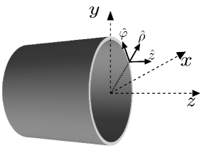
Figure 1: Cylindrical coordinate system in the nanotube.

For sufficiently thin tubes the demagnetizing field can be approximated by a local expression with the saturation magnetization acting as an effective radial hard axis anisotropy Carbou2001 ; Kohn2005 ; Goussev2014 . In this approximation and including exchange energy, uniaxial anisotropy energy, demagnetization energy and Zeeman energy, the micromagnetic energy can be written as Hubert ; Goussev2014

$$E=\int_{\Omega}d^{3}x(A|\nabla\vec{m}|^{2}+K_{u}(1-m_{z}^{2})+\frac{\mu_{0}M_{s}^{2}}{2}m_{\rho}^{2}-H_{a}m_{z}),$$ (5)

where $\Omega$ is the material volume of the nanotube, $A$ is the exchange constant, $K_{u}$ the uniaxial anisotropy and an external field $\vec{H}_{a}=H_{a}\hat{z}$ has been applied along the axis. The effective field is given by

$$\vec{H}_{\mbox{{\tiny eff}}}=-\frac{1}{\mu_{0}M_{s}}\frac{\delta E}{\delta\vec{m}}.$$

In a very thin nanotube variations of the magnetization with radius may be neglected so that the unit magnetization depends only on the polar coordinate $\varphi$ and the axial position $z$. With $\vec{m}=\vec{m}(\varphi,z)$, the effective magnetic field can be written as Goussev2014

$$\vec{H}_{e}=\frac{2A}{\mu_{0}M_{s}}\left[\frac{1}{R^{2}}\frac{\partial^{2}\vec{m}}{\partial\varphi^{2}}+\frac{\partial^{2}\vec{m}}{\partial z^{2}}\right]+\frac{2K_{u}}{\mu_{0}M_{s}}m_{z}\hat{z}-M_{s}m_{\rho}\hat{\rho}+H_{a}\hat{z}.$$ (6)

Introducing $M_{s}$ as unit of magnetic field, and introducing the dimensionless space and time variables $\xi=z/R$ and $\tau=\gamma_{0}M_{s}t$ we rewrite equations (1) and (6) in dimensionless form as

$$\frac{d\vec{m}}{d\tau}=-\vec{m}\times\vec{h}_{\mbox{{\tiny eff}}}+\alpha\vec{m}\times\frac{d\vec{m}}{d\tau}$$ (7)

with

$$\vec{h}_{\mbox{{\tiny eff}}}=A_{0}\left[\frac{\partial^{2}\vec{m}}{\partial\varphi^{2}}+\frac{\partial^{2}\vec{m}}{\partial\xi^{2}}\right]+k_{u}m_{z}\hat{z}-m_{\rho}\hat{\rho}+h_{a}\hat{z}$$ (8)

where $h_{a}$ is the dimensionless applied field. The dimensionless numbers that have appeared are $k_{u}=2K_{u}/(\mu_{0}M_{s}^{2})$ and $A_{0}$, the square of the ratio between the exchange length $l_{ex}=\sqrt{2A/\mu_{0}M_{s}^{2}}$ and the radius, that is, $A_{0}=2A/(\mu_{0}M_{s}^{2}R^{2})$. Equations (7) and (8) describe the dynamics of the problem.

Numerical simulations Yan2011 ; Hertel2016 have been performed for Permalloy for which the exchange constant $A=1.3\times 10^{-11}$ J m^-1, $M_{s}=8\times 10^{5}$A m^-1, $K_{u}\approx 0$ and the external applied field does not exceed $10^{-2}M_{s}$. The nanotube used in simulations has inner radius $R$, and width $w$ with $w<<R.$ Here we neglect the variations with radius and consider the range $R=55-100\times 10^{-9}$ m. The vacuum permeability $\mu_{0}=4\pi\times 10^{-7}$N A^-2 so that $\mu_{0}M_{s}\approx 1$T. We take the value $\gamma_{0}=2.21\times 10^{5}$ s^-1T^-1. For Permalloy the exchange length is $l_{ex}=5.68$ nm and for a radius of $80$ nm $l_{ex}/R=0.071$. The uniaxial anisotropy vanishes, $k_{u}=0$, and the dimensionless applied field is in the range $0<h_{a}<10^{-2}$. The damping parameter $\alpha$ in numerical simulations ranges from $0.01$ to $0.03$.

In the numerical simulations of Permalloy nanotubes Yan2011 ; Hertel2016 it is observed that a right handed vortex-type domain wall is stable against the Walker breakdown when driven with a magnetic field. The handedness of the domain wall in Yan2011 ; Hertel2016 is defined in relation to the applied field, a propagating domain wall is called right handed if $(\vec{m}\times\vec{H}_{a})\cdot\hat{\rho}>0$. Left handed domain walls become unstable and convert into the other, stable chirality. In this work we are interested in the speed of the stable DW, which will be selected through the scaling in the asymptotic solution.

III Asymptotic solution

In this section we perform an asymptotic analysis of the LLG equation to find a reduced model for the evolution of the domain wall as the applied field increases. The reduced model will be valid for a restricted parameter range which is chosen based on the numerical results described above for Permalloy. We are interested in right handed vortex walls for which the radial component of the magnetization is small, $m_{\rho}\ll 1$ Yan2011 ; Hertel2016 . Introducing a small dimensionless parameter $\epsilon$ we write this condition as

$$m_{\rho}=\epsilon\tilde{m}_{\rho}.$$ (9)

The normalization condition $\vec{m}^{2}=1$ becomes

$$m_{\varphi}^{2}+m_{z}^{2}=1-\epsilon^{2}{\tilde{m}_{\rho}}^{2}.$$ (10)

We will model a situation in which the ratio $l_{ex}/R$ and the Gilbert constant are of the same order in $\epsilon$ as the radial component of the magnetization. We assume that the applied field and uniaxial anisotropy are of an order smaller. Let then

$$A_{0}=\epsilon^{2}\tilde{A},\qquad k_{u}=\epsilon^{2}\tilde{k}_{u},\qquad h_{a}=\epsilon^{2}\tilde{h}_{a},\qquad\alpha=\epsilon\tilde{\alpha}.$$ (11)

It is found that a consistent asymptotic approach can be obtained if a new time scale $s=\epsilon\tau$ is introduced. With these scalings, the components of the effective magnetic field can be written as

$$\begin{split}(\vec{h}_{\mbox{{\tiny eff}}})_{\rho}&=-\epsilon\tilde{m}_{\rho}-2\epsilon^{2}\tilde{A}\frac{\partial m_{\varphi}}{\partial\varphi}+\epsilon^{3}\tilde{A}\left(\nabla_{s}^{2}\tilde{m}_{\rho}-\tilde{m}_{\rho}\right)\\ &=\epsilon H^{0}_{\rho}+\epsilon^{2}H^{1}_{\rho}+\epsilon^{3}H^{2}_{\rho},\end{split}$$ (12a)

$$\begin{split}(\vec{h}_{\mbox{{\tiny eff}}})_{\varphi}&=\epsilon^{2}\tilde{A}(\nabla_{s}^{2}m_{\varphi}-m_{\varphi})+2\epsilon^{3}\tilde{A}\frac{\partial\tilde{m}_{\rho}}{\partial\varphi}\\ &=\epsilon^{2}H^{1}_{\varphi}+\epsilon^{3}H^{2}_{\varphi},\end{split}$$ (12b)

$$(\vec{h}_{\mbox{{\tiny eff}}})_{z} =\epsilon^{2}\left(\tilde{h}_{a}+\tilde{A}\nabla_{s}^{2}m_{z}+\tilde{k}_{u}m_{z}\right)=\epsilon^{2}H^{1}_{z},$$ (12c)

where $\nabla_{s}^{2}=\partial_{\xi\xi}+\partial_{\varphi\varphi}$ and where we grouped terms according to the power of $\epsilon$ so that $H^{0}_{\rho}=-\tilde{m}_{\rho}$, $H^{1}_{\varphi}=\tilde{A}(\nabla_{s}^{2}m_{\varphi}-m_{\varphi})$ and $H^{1}_{z}=\tilde{h}_{a}+\tilde{A}\nabla_{s}^{2}m_{z}+\tilde{k}_{u}m_{z}.$ In obtaining these expressions for the effective field the property $\partial\hat{\rho}/\partial\varphi=\hat{\varphi},\,\partial\hat{\varphi}/\partial\varphi=-\hat{\rho}$ is used.

Introducing the scaling for $\alpha$ and $m_{\rho}$ in the LLG equation, we obtain at leading order in $\epsilon,$

$$\dot{\tilde{m}}_{\rho} =-(m_{\varphi}H_{z}^{1}-m_{z}H_{\varphi}^{1})+\tilde{\alpha}(m_{\varphi}\dot{m}_{z}-m_{z}\dot{m}_{\varphi}),$$ (13a)

$$\dot{m}_{\varphi} =-m_{z}H_{\rho}^{0},$$ (13b)

$$\dot{m}_{z} =m_{\varphi}H_{\rho}^{0},$$ (13c)

where a dot represents a derivative with respect to the scaled time variable $s$ and the subindices represent the components of each vector.

The normalization condition (10) implies that, at leading order, we may write

$$m_{\varphi}=\sin\theta(\xi,\varphi,s),\qquad\qquad m_{z}=\cos\theta(\xi,\varphi,s).$$ (14)

It follows then that equations (13b) and (13c) are equivalent and imply

$$\dot{\theta}=-H_{\rho}^{0}=\tilde{m}_{\rho}.$$ (15)

Replacing the value of $\tilde{m}_{\rho}$ from (15) in (13a) together with the expressions for the effective field $H_{\varphi}^{1},H_{z}^{1}$, the evolution equation for $\theta$ is found to be

$$\ddot{\theta}+\tilde{\alpha}\,\dot{\theta}=\tilde{A}\left(\theta_{\xi\xi}+\theta_{\varphi\varphi}\right)-\sin\theta\left(\tilde{h}_{a}+(\tilde{A}+\tilde{k}_{u})\cos\theta\right),$$ (16)

where the subscripts in $\theta$ denote derivatives with respect to $\xi$ and $\varphi$ respectively. Notice that one may go back to the original unscaled variables and the small parameter $\epsilon$ cancels out.

In what follows we study cylindrically symmetric domain walls, for which $\theta_{\varphi}=0$ and identify the evolution equation with the damped double Sine Gordon equation,

$$\frac{\partial^{2}\theta}{\partial\tau^{2}}+\alpha\frac{\partial\theta}{\partial\tau}=A_{0}\theta_{\xi\xi}-\sin\theta\left(h_{a}+(A_{0}+k_{u})\cos\theta\right),$$ (17)

a particular case of hyperbolic reaction diffusion equation, for which the existence and stability of traveling waves have been studied rigorously in Hadeler1988 ; Gallay2009 .

This equation has been derived in the analysis of domain wall propagation in weak ferromagnets, Gyorgy1968 ; Zvezdin1979 ; Mikeska1980 ; Papanicolaou1997 and in systems with a strong easy plane How1989 ; Wieser2010 . In Papanicolaou1997 the dependence of mobility on the Dzyaloshinskii constant is derived with great detail. A common feature in these problems is the sudden decrease in the rate of increase of the speed with the applied field.

This equation has the same traveling wave solutions as the reaction diffusion equation $\alpha\dot{\theta}=A_{0}\theta_{\xi\xi}-\sin\theta\left(h_{a}+(A_{0}+k_{u})\cos\theta\right)$ but with velocity $c=c_{\text{r}}/\sqrt{1+c_{\text{r}}^{2}/A_{0}}$ where $c_{\text{r}}$ is the speed of fronts of the reaction diffusion equation Hadeler1988 . We give the explicit expression for the head to head (HH) domain wall, the tail to tail solution is similar. The HH solution is found to be the usual domain wall profile,

$$\theta(\xi,t)=2\arctan\left[\exp\left(\frac{\xi-c\tau}{\Delta}\right)\right]$$ (18)

with the speed $c$ and domain wall width $\Delta$ given by

$$c=\sqrt{\frac{A_{0}}{A_{0}+k_{u}}}\,\,\frac{h_{a}}{\sqrt{\alpha^{2}+(A_{0}+k_{u})^{-1}\,h_{a}^{2}}},\qquad\Delta=\frac{\alpha c}{h_{a}}.$$ (19)

The leading order magnetization $\vec{m}=m_{\varphi}\hat{\varphi}+m_{z}\hat{z}$ is given by

$$\vec{m}=\sech\left(\frac{\xi-c\tau}{\Delta}\right)\hat{\varphi}-\tanh\left(\frac{\xi-c\tau}{\Delta}\right)\hat{z}.$$ (20)

The external field is applied along the $z$ axis so the magnetization is a right handed ($m_{\varphi}\geq 0$) head to head domain wall as defined in Hertel2016 . The small radial component of the magnetization is calculated from (15).

For small applied field we recover the linear regime, that is, the speed increases linearly with the field, and the domain wall width tends to a constant value, that is,

$$\lim_{h_{a}\rightarrow 0}\,c=\sqrt{\frac{A_{0}}{A_{0}+k_{u}}}\,\,\frac{h_{a}}{\alpha},\quad\lim_{h_{a}\rightarrow 0}\,\Delta=\sqrt{\frac{A_{0}}{A_{0}+k_{u}}}.$$ (21)

In this limit the dynamics is primarily governed by the reaction diffusion equation $\alpha\theta_{\tau}=A_{0}\theta_{\xi\xi}-\sin\theta\left(h_{a}+(A_{0}+k_{u})\cos\theta\right)$ as already found in Goussev2014 .

In terms of the physical parameters the dimensional domain wall width for small field $\delta=\Delta R$ and speed $v_{L}$ can be written as

$$\delta=\sqrt{\frac{A}{\frac{A}{R^{2}}+K_{u}}},\qquad v_{L}=\gamma_{0}\frac{H_{a}}{\alpha}\delta$$

For Permalloy, $K_{u}=0$ and $\delta=R$ in agreement with the results for a static domain wall in a thin nanotube La2010 . The speed $v_{L}$ coincides with the low field Walker solution $v_{W}=\gamma_{0}H_{a}\sqrt{A/K}/\alpha$, with $K$ an effective anisotropy $A/R^{2}$. In the limit of large radius the domain wall width for an in plane magnetized thin film, $\sqrt{A/K_{u}}$ is recovered.

For large applied field the speed tends to a constant value and the domain wall width decreases as the field increases,

$$\lim_{h_{a}\rightarrow\infty}\,c=\sqrt{A_{0}}\quad\lim_{h_{a}\rightarrow\infty}\,\Delta=\frac{\alpha\sqrt{A_{0}}}{h_{a}}.$$ (22)

This limiting value for the speed corresponds to the minimal value of the phase velocity for spin waves, $v_{p_{\text{\tiny{min}}}}$. In effect, consider a material like Permalloy with vanishing uniaxial anisotropy for simplicity. The dispersion relation for the DSG equation (17), for vanishing damping and vanishing applied field, is given by $\omega_{\text{\tiny DSG}}=\sqrt{A_{0}}\sqrt{1+k^{2}}$, so that the phase speed is a decreasing function of $k$ which tends asymptotically to $\sqrt{A_{0}}$ as $k$ grows. The full dispersion relation for spin waves in a thin nanotube, in the absence of damping and applied field, with vanishing uniaxial anisotropy, is given by GoLaNu2010

$$\omega=\frac{\sqrt{A_{0}}}{2}\sqrt{(1+k^{2})+A_{0}(1+k^{2})^{2}}$$ (23)

in the units used in this work. We see that for small $A_{0}$ the full dispersion relation coincides, up to a constant, with $\omega_{\text{\tiny DSG}}$.

The evolution equation (17) shows the transition from the low field regime where the speed of the domain wall increases linearly with the field to the regime where the domain wall speed approaches $v_{p_{\text{\tiny{min}}}}$ and is slowed down by emitting spin waves. In order to capture the large applied field regime where the DW speed exceeds $v_{p_{\text{\tiny{min}}}}$ and Cherenkov emission occurs a different scaling is needed. The DW width shrinks with increasing field, $\Delta\approx\alpha\sqrt{A_{0}}/h_{a}$, which indicates that at larger fields a new scaling for the longitudinal coordinate $\xi$ is required. The damped DSG equation captures the emission of spin waves that occurs below but close to $v_{p_{\text{\tiny{min}}}}$.

A different transition occurs at $h_{a}^{\text{\tiny{KPP} }}=2A_{0}$ when the speed of the reaction diffusion equation $c_{r}$ changes from a pushed to a pulled or KPP front DepassierEPL and $c_{r}$ becomes proportional to the square root of the applied field.

In what follows consider Permalloy for which $k_{u}=0$. Going back to dimensional quantities, the speed of the domain wall for Permalloy is given by Eq. (2) with the limiting values at low and high fields Eq. (3) and Eq. (4). In Fig. 2 the graph of the speed as a function of the applied field shows the gradual change from the linear to the magnonic regime. We have used the values given above for Permalloy.

Figure 2: Speed of the domain wall versus applied field in millitesla for a thin Permalloy nanotube of radius $R=55$ nanometers. At low field the speed increases linearly with the field, after a sudden change in slope the speed tends to a constant value $v_{\infty}$ at large fields. The dashed lines show the limiting speeds $v_{\text{L}}$ and $v_{\infty}$.

An approximate estimate of the field $H_{a}^{*}$ at which this transition occurs is obtained by the intersection $v_{\text{L}}(H_{a}^{*})=v_{\infty}$ which yields

$$H_{a}^{*}=\frac{\alpha}{R}\sqrt{\frac{2A}{\mu_{0}}}.$$

For Permalloy we obtain $v_{\infty}=1006$ m s^-1, and $B_{a}^{*}=\mu_{0}H_{a}^{*}=0.001$ T. The transition to the KPP regime occurs at a much higher field, $B_{a}^{\text{\tiny{KPP} }}=\mu_{0}H_{a}^{\text{\tiny{KPP} }}=0.021$ T and is not associated to the transition from the linear to the magnonic regime. In this simple model the order of magnitude of the speed and the value of the field at which the transition from the linear to the magnonic regime occurs agrees with the order of magnitude of the numerical simulations of the LLG equation.

IV Summary

We studied the dynamics of a vortex domain wall in a thin nanotube by means of an asymptotic study of the Landau-Lifshitz Gilbert equation in a parameter regime based on existing numerical simulations Yan2011 ; Hertel2016 . The numerical simulations on Permalloy nanotubes in a certain range of radii showed that when an external field is applied along the axis, domain walls of one type of chirality, for which the radial magnetization remains small during the motion, are stable and can reach high speeds. Initially the speed increases linearly with the applied field, and at higher fields the rate of increase is slowed down by the emission of spin waves. No Walker breakdown was observed in the parameter range considered in the numerical studies. Domain walls of the opposite chirality are unstable and as the field increases they convert into DW of stable chirality.

The purpose of this work was to understand analytically the behavior of the speed of domain walls of stable chirality as a function of the applied field. Through an asymptotic analysis the LLG was reduced to the damped double sine-Gordon equation from which an explicit analytic formula for the speed as a function of the applied field was obtained together with the leading order DW profile. This model captures the initial regime of linear growth of the speed followed by a slowdown in the rate of increase through the emission of spin waves before reaching the minimal phase speed of the spin waves, which is an upper bound on the speed of the DW in this model. The order of magnitude of the speed and the value of the applied field where the transition from the linear to the magnonic regime occurs is in agreement with the numerical results of Yan2011 ; Hertel2016 . In order to reach higher fields and capture the Cherenkov spin wave emission process a different asymptotic regime is necessary.

For Permalloy, which has vanishing uniaxial anisotropy, the ratio of the exchange constant with the square of the radius of the nanotube $A/R^{2}$ plays the role of an effective uniaxial anisotropy which leads to a mobility proportional to the nanotube radius. In constrast, for weak ferromagnets the mobility is proportional to de Dzyaloshinkii-Moriya constant. That the effect of curvature acts as an equivalent effective anisotropy was already shown in Goussev2014 ; Gaididei2014 , and an analogy between the effect of DMI and curvature was found in the dispersion relation of spin waves in a nanotube Ot2016 . The results in this manuscript show a similar effect when studying the transition from the linear to the magnonic DW regime in nanotubes.

An analytical approach to the regime of higher field, where Cherenkov emission occurs, will be the subject of future study.

V Acknowledgments

This work was partially supported by Fondecyt (Chile) project 116–0856.

References

- (1) L. D. Landau and E. M. Lifshitz, Phys. Z. Sowjet., 8, 153 (1935).
- (2) T. L. Gilbert, Ph.D. Thesis, Illinois Institute of Technology (1956), partially reprinted in IEEE Trans. Mag., 40, 3443 (2004).
- (3) L.R. Walker, Bell Telephone Laboratories Memorandum, 1956 (unpublished). An account of this work is given in J.F. Dillon, Jr., Magnetism, Vol. III, edited by G.T. Rado and H. Suhl (Academic, New York, 1963).
- (4) N. L. Schryer and L. R. Walker, J. Appl. Phys. 45, 5406 (1974).
- (5) M. Yan, A. C. Kákay, F. García-Sanchez and R. Hertel, Appl. Phys. Lett. 99, 122505 (2011).
- (6) R Hertel, J. Phys.: Condens. Matter 28, 483002 (2016).
- (7) R. Hubert, A. Schäfer, Magnetic Domains (Springer-Verlag Berlin Heidelberg, 1998).
- (8) A. Goussev, J. M. Robbins and V. Slastikov, EPL 105, 67006 (2014).
- (9) E. M. Gyorgy, and F. B. Hagedorn, J. Appl. Phys. 39, 88 (1968).
- (10) A. K. Zvezdin, JETP Letters 29 513 (1979).
- (11) N. Papanicolaou, Phys. Rev. B 55, 12290-12308 (1997).
- (12) E. G. Galkina and B. A. Ivanov, Low Temp. Phys. 44 618 (2018).
- (13) Y. Nakatani, A. Thiaville and J. Miltat, Nature Materials 2, 521 (2003).
- (14) A. Thiaville and Y. Nakatani, Domain-Wall Dynamics in Nanowires and Nanostrips in: Hillebrands B., Thiaville A. (Eds) Spin Dynamics in Confined Magnetic Structures III. Topics in Applied Physics, vol 101. Springer, Berlin, Heidelberg (2006).
- (15) R. Wieser, U. Nowak and K. D. Usadel, Phys. Rev. B 69, 064401 (2004).
- (16) R. Wieser, E. Y. Vedmedenko and R. Wiesendanger, Phys. Rev. B 81, 024405 (2010).
- (17) X. S. Wang and X. R. Wang, Phys, Rev. B 90 184415 (2014).
- (18) D. Bouzidi and H. Suhl, Phys. Rev. Lett. 65 2587 (1990).
- (19) I. A. Akhiezer and A. E. Borovik, Soviet Phys. JETP 25 885 (1967).
- (20) V. G. Baryakhtar, B. A. Ivanov and M. V. Chetkin, Sov. Phys. Usp. 28, 563 (1986).
- (21) A. Goussev, J. M. Robbins, V. Slastikov and O. A. Tretiakov, Phys. Rev. B 93 054418 (2016).
- (22) Y. Gaididei, V.P. Kravchuk and D. D. Sheka, Phys. Rev. Lett. 112 257203 (2014).
- (23) J. A. Otálora, M. Yan, H. Schultheiss, R. Hertel and A. Kákay, Phys. Rev. Lett. 117, 227203 (2016).
- (24) M. Staňo and O. Fruchart, Ch. 3 of Handbook of Magnetic Materials vol. 27, North Holland (Elsevier), pp. 155-267 (2018).
- (25) G. Carbou, Math. Models Methods Appl. Sci., 11, 1529 (2001).
- (26) R. V. Kohn and V. Slastikov , Arch. Ration. Mech. Anal., 178, 227 (2005).
- (27) K. P. Hadeler, Proc. Edinburgh Math. Soc. 31, 89-97 (1988).
- (28) T, Gallay and R. Joly, Ann. Sci de l’Ecole Normale Supérieure, 42, 103-140 (2009).
- (29) H. J. Mikeska, J. Phys. C 13, 2913 (1980).
- (30) H. How, R. C. O’Handley and F. R. Morgenthaler, Phys. Rev. B 40, 4808 (1989).
- (31) P. Landeros and A. S. Nuñez, J. Appl. Phys. 108 033917 (2010).
- (32) A. L. González, P. Landeros and A. S. Núñez, J. Mag. Mag. Mater. 322, 530 (2010).
- (33) M. C. Depassier, EPL 108, 37008 (2014).