Learning Effective RGB-D Representations for Scene Recognition

Abstract

Deep convolutional networks (CNN) can achieve impressive results on RGB scene recognition thanks to large datasets such as Places. In contrast, RGB-D scene recognition is still underdeveloped in comparison, due to two limitations of RGB-D data we address in this paper. The first limitation is the lack of depth data for training deep learning models. Rather than fine tuning or transferring RGB-specific features, we address this limitation by proposing an architecture and a two-step training approach that directly learns effective depth-specific features using weak supervision via patches. The resulting RGB-D model also benefits from more complementary multimodal features. Another limitation is the short range of depth sensors (typically 0.5m to 5.5m), resulting in depth images not capturing distant objects in the scenes that RGB images can. We show that this limitation can be addressed by using RGB-D videos, where more comprehensive depth information is accumulated as the camera travels across the scenes. Focusing on this scenario, we introduce the ISIA RGB-D video dataset to evaluate RGB-D scene recognition with videos. Our video recognition architecture combines convolutional and recurrent neural networks (RNNs) that are trained in three steps with increasingly complex data to learn effective features (i.e. patches, frames and sequences). Our approach obtains state-of-the-art performances on RGB-D image (NYUD2 and SUN RGB-D) and video (ISIA RGB-D) scene recognition.

I Introduction

The goal of scene recognition is to predict scene labels for visual data such as images and videos. Success in visual recognition mainly depends on the features used to represent the input data. Scene recognition in particular has benefited from recent developments in data-driven representation learning, where massive image datasets (ImageNet and Places [1]) provide the necessary amount of data to effectively train complex convolutional neural networks (CNNs) [2, 3] with millions of parameters. The features extracted from models pretrained with those datasets are generic and powerful enough to obtain state-of-the-art performance in relevant scene benchmarks (e.g., MIT indoor 67 [4], SUN397 [5]), just using an SVM [6] or fine-tuning, and outperforming earlier handcrafted paradigms (e.g., SIFT, HOG, bag-of-words).

In parallel, low cost depth sensors can capture depth information that complements RGB data. Depth can provide valuable information to model object boundaries and understand the global layout of the scene. Thus, RGB-D models should improve recognition over mere RGB models. However, RGB-D data needs to be captured with a specialized and relatively complex setup [7, 8] (in contrast to RGB data that can be collected by crawling the web). For this reason, RGB-D datasets are orders of magnitude smaller than the largest RGB datasets, also with much fewer categories. Since depth images somewhat resemble some aspects of RGB images (specially in certain color codings), shapes and objects can be often identified in both RGB and depth images (see Fig. 2). This motivates the common practice of leveraging the architecture and parameters of a deep network pretrained on large RGB datasets (e.g., ImageNet, Places) to then fine tune two separate RGB and depth branches with the corresponding modality-specific images from the target set. The two branches are then combined in the final RGB-D model. This is the main approach used in recent works [8, 9, 10, 11, 12, 13].

However, relying on networks trained for RGB data to build depth features seems to be an inherent limitation. The question is whether fine tuning is the best possible solution given the limited depth data. Here we challenge the usual assumption that learning depth features from scratch with current limited data is still less effective. In fact, we show that a significantly smaller network trained in a two-step process with patches pretraining via weak supervison can effectively learn more powerful depth features, more complementary to RGB ones, and thus provide higher gains in RGB-D models. We show that this weakly-supervised pretraining stage is critical to obtain powerful depth representations, even more effective than those transferred from deeper RGB networks.

A second limitation of current RGB-D scene recognition on images is the limited range of depth cameras, in addition to less accurate information with distance. For instance, the effective range of the depth sensor of the widely used Microsoft Kinect is 0.5m to 5.5m, with accuracy decreasing with distance. This leads to much more limited information and to ambiguity in the classification than in the case of RGB images (see Fig. 1, where furniture store and classroom can be easily confused with bedroom and conference room, respectively, due to the limited information about distant objects). In addition, images are also limited to capture only a fraction of large scenes. Videos can alleviate these problems by traversing the scene, and increasing the overall coverage of visual information. Motivated by these limitations, we introduce a new RGB-D video database for scene recognition (ISIA RGB-D).

We take advantage of the richer depth (and RGB) information in videos and address RGB-D video scene recognition extending the scene recognition architecture for images with a recurrent neural network (RNN) in order to obtain a richer spatio-temporal embeddings. Since the training RGB-D data is limited, we propose a three-steps training procedure: 1) weakly-supervised pretraining of CNNs with depth data, 2) pretraining of temporal embedding with frames, and 3) joint spatio-temporal fine tuning.

A preliminary version of this work was presented in [14], which mainly focuses on addressing the problem of limited depth data for RGB-D scene recognition. In this paper we extend that work to address the problem of fully capturing depth information in wide scenes, since depth cameras only capture depth information in a short range. We introduce the ISIA RGB-D video database to study scene recognition under these settings. We propose a CNN-RNN framework to model and recognize RGB-D scenes. Inspired by the effectiveness of the two-step training strategy in the still image case (pretraining with patches followed by fine tuning with full images), we further propose a three-step training procedure for the CNN-RNN architecture. Our evaluations show significant gains obtained when integrating depth video in comparison to still images.

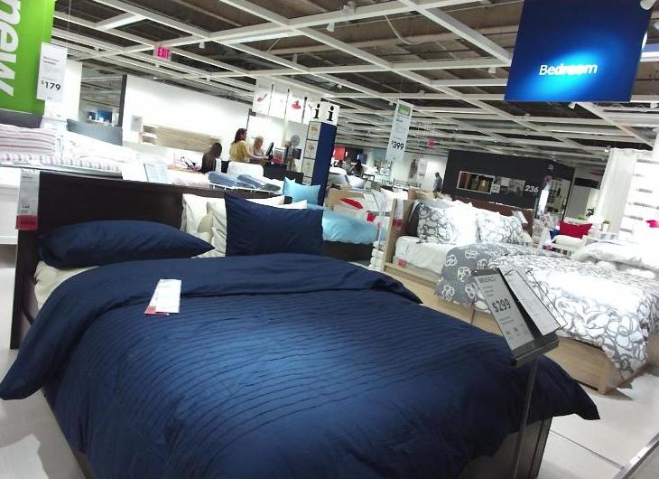
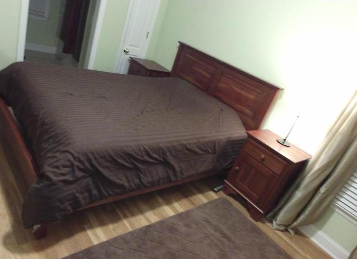
		RGB
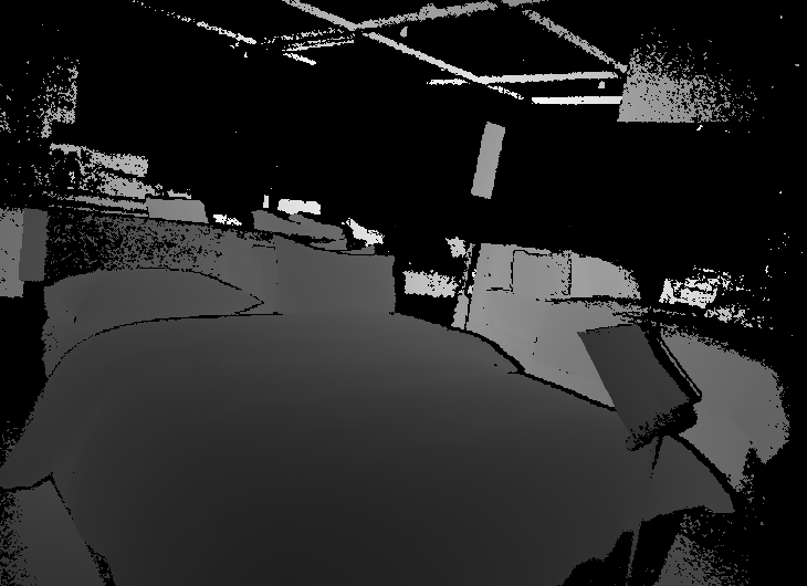
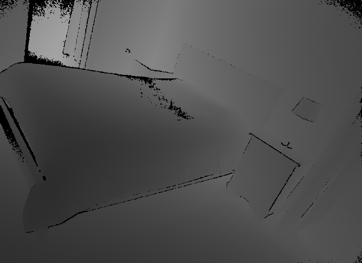
		Depth
(a) Furniture store	(b) Bedroom
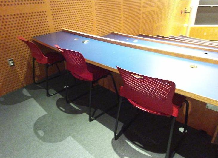
		RGB
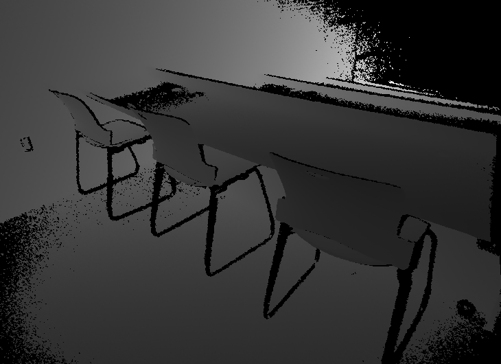
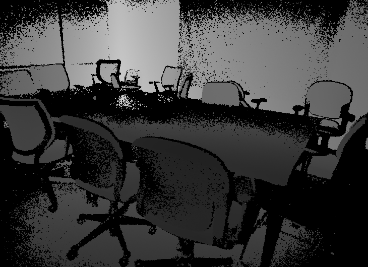
		Depth
(c) Classroom	(d) Conference room

Figure 1: Pairs of RGB-D images from the SUN RGB-D database. Black pixels represent regions where depth information is not available, where the objects are too far to be captured by depth cameras (but not by RGB cameras). This loss of depth information can lead to category confusion in depth images, e.g., (a) furniture store vs (b) bedroom, (c) classroom vs (d) conference room.

II Related Work

II-A RGB-D scene recognition

Earlier works use handcrafted features, engineered by experts to capture some specific properties considered representative. Gupta et al. [15] propose a method to detect contours on depth images for segmentation, then further quantize the segmentation outputs as local features for scene classification. Banica et al. [16] quantize local features with second order pooling, and use the quantized feature for segmentation and scene classification. More recently, multi-layered neural networks can learn features directly from large amounts of data. Socher et al. [17] use a single layer CNN trained unsupervisedly on patches, and combined with a recurrent neural network (RNN). Gupta et al. [18] use R-CNN on depth images to detect objects in indoor scenes. Since the training data is limited, they augment the training set by rendering additional synthetic scenes.

Current state-of-the-art relies on transferring and fine tuning Places-CNN to RGB and depth data [11, 9, 10, 8]. Wang et al. [9] extract deep features on both local regions and whole images on both RGB, depth and surface normals, and then use component-aware fusion to combine these multiple components. Some approaches [10, 11] propose incorporating CNN architectures to jointly fine tune RGB and depth image pairs. Zhu et al. [10] jointly fine tune the RGB and depth CNN models by including a multi-modal fusion layer, simultaneously considering inter and intra-modality correlations, meanwhile regularizing the learned features to be compact and discriminative. Alternatively, Gupta et al. [11] propose a cross-modal distillation approach where learning of depth filters is guided by the high-level RGB features obtained from the paired RGB image. Note that this method makes use of additional unlabeled frames during distillation.

In this paper we avoid relying on large yet still RGB-specific models to obtain depth features, and train depth CNNs directly from depth data, learning truly depth-specific and discriminative features, compared with those transferred and adapted from RGB models.

II-B Weakly-supervised CNNs

Accurate annotations of the objects (i.e. category and bounding boxes) in a scene are expensive and often not available. However, image-level annotations (e.g., category labels) are cheaper to collect. These weak annotations have been used recently in weakly supervised object detection frameworks [19, 20, 21]. Oquab et al. [21] propose an object detection framework to fine tune pretrained CNNs with multiple regions, where a global max-pooling layer selects the regions to be used in fine tuning. Durand et al. [19] extend this idea by selecting both useful (positive) and "useless" (negative) regions with a maximum and minimum mixed pooling layer. Bilden and Vedaldi [20] use region proposals to select regions. Weakly supervised learning has been also used in RGB scene recognition [22, 23, 24, 25, 26, 27]. Similarly to the previous case, image-level labels are used to supervise the learning of mid-level features localized in smaller regions. For example, the classification model of [23] is trained with patches that inherit the scene label of the images. That training process is considered as weak supervision since patches with similar visual appearances may be assigned different scene labels.

These works often rely on CNNs already pretrained on large RGB datasets, and weak supervision is used in a subsequent fine tuning or adaptation stage to improve the final features for a particular task. In contrast, our motivation is to train depth CNNs when data is very scarce, with a weakly supervised CNN for model initialization. In particular, we pretrain the convolutional layers prior to fine tuning with full images.

II-C Scene recognition on sequential data

Previous works on scene recognition with videos focus on RGB data [28, 29, 30]. Moving vistas [30] focuses on scenes with highly dynamic patterns, such as fire, crowded highways or waterfalls, using chaos theory to capture dynamic attributes. Derpanis et al. [29] study how appearance and temporal dynamics contribute to scene recognition. Feichtenhofer et al. [28] propose a new dataset with more categories and an architecture using residual units and convolutions across time. However, none of these video databases have depth data, and also these databases contain outdoor natural scenes where is difficult to capture depth information.

There are some datasets involving RGB-D videos of scenes. The SUN3D database [31] contains videos of indoor scenes primarily to study structure from motion and semantic segmentation. The NYUD2 dataset [32] contains videos with some images annotated scene labels and with semantic segmentations. However, it contains 27 categories but only 10 are well represented, of which one or two categories could be considered wide scenes (e.g., furniture store). In this paper we focus more on wide scenes, which can benefit more from traversing the scene, and propose a new dataset better suited to study RGB-D scene recognition in videos.

II-D Embedding sequential data

Recent works on visual recognition with videos incorporate spatio-temporal deep models. Action recognition is an example that requires modeling appearance and temporal dynamics. Many works in this area use spatio-temporal CNN models [33] or two stream combining appearance and motion [34, 35]. Feichtenhofer et al. [28] propose to extend the two stream CNN with a ResNet architecture [36] and apply it to scene recognition.

III Depth Features from RGB Features

Deep CNNs trained with large datasets can extract excellent representations that achieve state-of-the-art performance in a wide variety of recognition tasks [6]. In particular, those trained with the Places 205 database (hereinafter Places-CNN) are essential to achieve state-of-the-art scene recognition accuracy [1], even simply using a linear classifier or fine tuning the parameters of the CNN. This knowledge transfer mechanism has been used extensively (e.g., domain adaptation) but mostly within the RGB modality (intra-modal transfer). Therefore, it is not clear its effectivity with depth (cross-modal transfer).

Similarly to RGB features, depth features can be handcrafted or learned from data. Since there is no large dataset of depth images, the common approach is to transfer RGB features from deep RGB CNNs, due to certain similarities between both modalities (see Fig. 1 and 2).

In this section we compare intra-modal and cross-modal transfer of a Places-CNN to RGB and depth, respectively, analyze its limitations and explore other combinations of transfer and learning to learn better depth features.

III-A Places-CNN for RGB and depth data

We focus first on the first convolutional layer (conv1), since it is the closest to the input data and therefore essential to capture modality-specific patterns.

Fig. 2 (top) shows the average activation ratio (in descending order) of the 96 filters in the layer conv1 of a Places-CNN with AlexNet architecture [2]. Activation rate here indicates how often the response of a particular filter is non-zero. When the input data is the validation set of Places 205 (i.e., same input distribution as in the source training set), the curve is almost flat, showing that the network is well designed and trained, with all the filters contributing almost equally to build discriminative representations. When the input is from other RGB scene datasets, such as 15 scenes [37], MIT Indoor [4] and the RGB images from SUN RGB-D [8], the curves are very similar, i.e., a flat activation rate for most filters and just a few filters with higher or lower activation rate, due mostly to the particular biases of the datasets. This shows the majority of the filters in conv1 are good representations of the low-level patterns in RGB scenes (see Fig. 2 middle). This is reasonable, since these patterns are observed in similar proportions in both the source and target datasets.

Now let us consider the same SUN RGB-D dataset as input data, but depth images instead of RGB (in HHA encoding, see Fig. 2 bottom). While still representing the same scenes, the activation rate curve shows a completely different behavior, with only a subset of the filters being relevant and a large number being rarely activated. This illustrates how RGB and depth modalities are significantly different at the low-level. In HHA encoded depth images we can still observe edges and smooth gradients, but other patterns such as texture are simply not present in that modality (observe in Fig. 2 bottom how the textures in the newspaper and the chair back completely disappear in HHA images). This can be observed more clearly by rearranging the filters according to decreasing activation rate with HHA images (see Fig. 2 middle), and see how the most frequently activated filters are typically those dealing with smooth color variations and edges (yet not optimal), while the least activated deal with RGB-specific features such as Gabor-like and high frequency patterns.

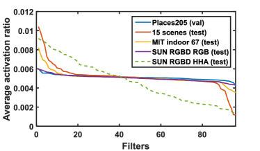
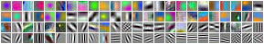
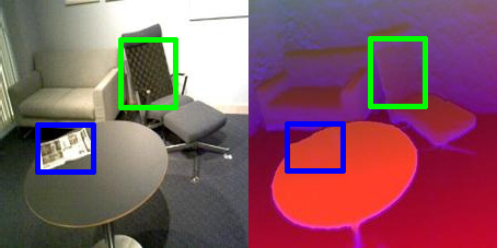
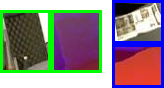
Figure 2: Patterns in RGB and depth modalities. Top: average nonzero activations of the filters in the conv1 layer of Places-CNN on different scene datasets. Middle: Conv1 filters ordered by mean activation on SUN RGB-D HHA. Bottom: examples of scenes captured in RGB and depth (HHA encoding) with textured regions highlighted.

III-B Fine tuning with depth data

The previous result suggests that adapting bottom layers is more important when transferring to depth. In previous works [8, 9, 10, 12, 13] the depth network is fine tuned only in the top layers as a whole, but with such limited data it will still have difficulty to reach and properly adapt the bottom layers. In contrast, we want to emphasize explicit adaptation in bottom layers, since they are more critical to capture modality-specific patterns.

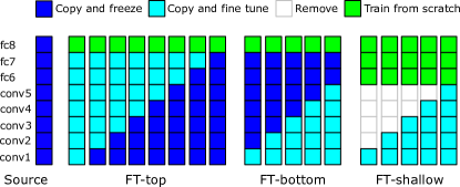
Figure 3: Different settings for learning depth features, combining transfer from a source Places-CNN (AlexNet architecture), fine tuning and training from scratch: (a) top layers, (b) bottom layers, and (c) bottom layers with some intermediate convolutional layers removed. Each column represents a particular setting.

Here we explore alternatives to learn depth representations, considering several factors: parameter initialization and tuning (trained from scratch, fine tuned or frozen), the position of the trainable/tunable layers (top or bottom), and the overall depth of the network. With this in mind, we organize these settings in three groups (see Fig. 3, where each column represents a particular setting): a) FT-top: the conventional method where only a few layers at the top are fine tuned, b) FT-bottom: where a few layers at the bottom are fine tuned, and c) FT-shallow: a few convolutional layers are kept and fine tuned while the others are removed. Note that fc8 is always trained, since it must be resized according to the target number of categories. In FT-shallow we also train the other two fully connected layers.

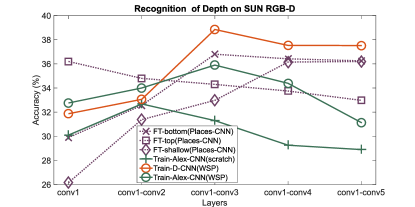
Figure 4: Comparison of different fine tuning and training strategies evaluated on SUN RGB-D (depth images). The figure includes curves for methods based on fine tuning Places-CNN (see Fig. 3) and for methods based on training from scratch (see Fig. 6). The horizontal axis shows the number of convolutional layers being trained (scratch) or fine tuned.

The classification accuracy on the depth data of the SUN RGB-D dataset is shown Fig. 4. We first analyze the three FT-curves (i.e. FT-bottom, FT-keep, FT-WSP and FT-top, also see Fig. 3), obtained by transferring and fine tuning Places-CNN. Fine tuning top layers (FT-top) does not help significantly until including bottom convolutional layers, which contrasts with RGB where fine tuning one or two top layers is almost enough to reach the maximum gain [38]. Further extending fine tuning to bottom layers in RGB helps very marginally. This agrees with the previous observation that bottom layers and conv1 in particular need to be adapted to the corresponding modality. In fact, fine tuning only the three bottom layers (FT-bottom) achieves 36.5% accuracy which is higher than fine tuning the whole network, probably due to overfitting. We also evaluated shallower networks with fewer convolutional layers and therefore fewer parameters (FT-shallower), where we observe again that fine tuning the first layers contributes most to high accuracy. Again, these results suggest that adapting bottom layers is much more important when transferring RGB to depth, and therefore that fine tuning for intra-modal and cross-modal transfer should be handled differently.

III-C More insight from layer conv1

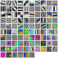
(a)	(b)
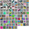
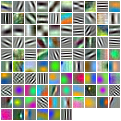
(c)	(d)
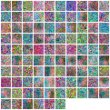
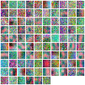
(e)	(f)
(g)	(h)

Figure 5: Visualizing the first convolutional layer (conv1): (a) Places-CNN; (b) full fine tuned Places-CNN; (c) FT-bottom (Places-CNN); (d) FT-shallower (Places-CNN), conv1; (e) Train-Alex-CNN (scratch); (f) Train-Alex-CNN (WSP), training with patches ($99\times 99$ pixels); (g) WSP-CNN, kernel size $5\times 5$ pixels, training with patches ($35\times 35$ pixels); (h) Train-D-CNN (WSP). All methods are trained/fine tuned using only the depth data from SUN RGB-D.

We can compare the filters obtained in conv1 with these different settings for additional insight (see Fig. 5). Although there is some gain (when fine tuning) in accuracy, only a few particular filters have noticeable changes during the fine tuning process (see Fig. 5 from (a) to (d)). This suggests that the CNN is still mainly reusing the original RGB filters, and thus trying to find RGB-like patterns in depth data. As Fig. 2 middle shows, a large number of filters from Places-CNN are significantly underused on depth data (while they are properly used on RGB data). These observations suggest that reusing Places-CNN filters for conv1 and other bottom layers may not be a good idea. Moreover, since filters also represent tunable parameters, this results in a model with too many parameters that is difficult to train with limited data.

IV Learning effective depth features

In the previous section, it can be observed that transferring and fine tuning Places-CNN with depth data is somewhat effective but limited to exploiting some specific RGB-like patterns in depth images. It also can be observed that bottom layers seem to be the most important when learning modality-specific features. Here we aim at learning depth-specific features of early convolutional layers, directly from depth data, that are at least competitive in performance with those transferred from Places-CNN. The main problem is the limited depth data and the complexity of Places-CNN (i.e., large number of parameters).

IV-A Weak supervision on patches

We propose to work on patches instead of full images and adapt the complexity of the network to accommodate smaller feature maps and the amount of training data. In this sense we can increase the training data while reducing the number of parameters, which will help to learn discriminative filters in the first convolutional layers. Since patches typically cover objects or parts of objects, in principle the original scene labels are not suitable for supervision. For instance, the scenes categories living room, dining room, and classroom often contain visually similar patches since they may represent mid-level concepts such as walls, ceilings, tables and chairs, but suitable mid-level labels or object annotations are not available. However, a particular patch can be weakly labeled with the corresponding scene category of the image. This weak supervision has been proved helpful to learn discriminative features for RGB scene recognition [22, 39, 25, 27]. Hence, we refer to this network as weakly supervised patch-CNN (WSP-CNN). Once the network is trained, the parameters of the WSP-CNN are used to initialize the convolutional layers of the full network, which is then fine tuned with full images.

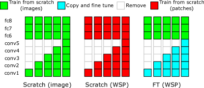
Figure 6: Training strategies for Alex-CNN variants with depth images, (a) from scratch, (b) weakly-supervised with patches, and (c) fine-tuned after weakly supervised training with patches.

We first implement this strategy on the AlexNet architecture (hereinafter Alex-CNN). We sample a grid of $4\times 4$ patches of $99\times 99$ pixels for weakly-supervised pretraining. When switching from WSP-CNN to Alex-CNN, only the weights of the convolutional layers are transferred. Fig. 4 shows that using this pretraining stage significantly outperforms training directly with full images (compare Train-Alex-CNN (WSP) vs Train-Alex-CNN (scratch)). Furthermore, in the conv1 filters shown in Fig. 5f (WSP) the depth specific-patterns are much more evident than in Fig. 5e (full image). Nevertheless, they still show a significant amount of noise (probably remnant of the original random initialization which still cannot vanish with such limited training data). This suggests that AlexNet is still too complex, and perhaps the size of Alex-CNN kernels may be too large for depth data.

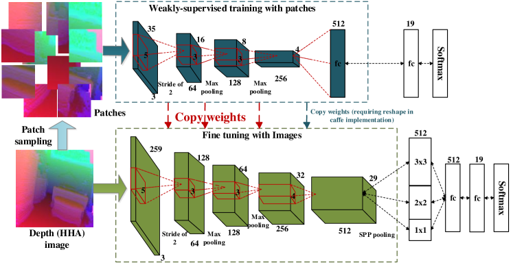
Figure 7: Two-step learning of depth CNNs combining weakly supervised pretraining and fine tuning.

IV-B Interpretation as category co-occurrence modeling

Our approach can be seen as a first set of layers that learns an intermediate local semantic representation (e.g., objects, regions), while the other set of layers corresponds to a second model that infers scenes from a set of intermediate representation. This actually resembles earlier two-step local-to-global approaches to scene recognition using intermediate representations (e.g., bag-of-words, topic models).

In particular, a weakly supervised model followed by a global model resembles previous works on scene category co-occurrence modeling [22, 25]. Supervised by global labels, the model can predict scene categories directly (e.g., pooling the outputs of the softmax) [22]. However, the weak supervision with scene categories makes the prediction very ambiguous, resulting in visually related categories predicted with similar probabilities due to lack of global context. Luckily, these co-occurrence patterns are consistent across categories, so the second model exploits them to resolve the ambiguity [25], often combined with spatial and multi-feature contexts [39, 27].

In contrast to previous works about category co-occurrences, we do not use probabilities as intermediate representations, but the activations before the softmax. This makes training easier. In general, all layers in deep networks can be trained jointly, as long as the training data is enough. However, when training data is limited, this two-step procedure with weak supervision seems to be very helpful.

IV-C Depth-CNN

Since the complexity and diversity of patterns found in depth images are significantly lower than those found in RGB images (e.g., no textures), we reduced the number of convolutional layers to three and also the size of the kernels in each layer (see Fig 7 top for the details). The sizes of the kernels are $5\times 5$ (stride 2), $3\times 3$ and $3\times 3$, and the size of max pooling is $2\times 2$, stride 2. We sample a grid of $7\times 7$ patches of $35\times 35$ pixels for weakly-supervised pretraining.

Fig 7 bottom shows the full architecture of the proposed depth-CNN (D-CNN). After weakly supervised pretraining, we transfer the weights of the convolutional layers. The output of conv4 in D-CNN is $29\times 29\times 512$, almost 50 times larger than the output of pool5 (size of $6\times 6\times 256$) in Alex-CNN, which leads to 50 times more parameters in this part. In order to reduce the number of parameters in the next fully connected layer, we include a spatial pyramid pooling (SPP) [40] composed of three pooling layers of size of $29\times 29$,$15\times 15$, $10\times 10$. SPP also captures spatial information and allows us to train the model end-to-end. This model outperforms Alex-CNN, both fine tuned and weakly-supervised trained (see D-CNN (WSP) in Fig. 4). Comparing the visualizations in Fig. 5, the proposed WSP-CNN and D-CNN learn more representative kernels, which also helps to improve the performance. This also suggests that smaller kernel sizes are more suitable for depth data since high frequency patterns requiring larger kernels are not characteristic of this modality.

V Multimodal RGB-D architecture

Most previous works use two independent networks for RGB and depth, that are fine tuned independently, then another stage exploits correlation between RGB and depth features and finally another stage learns the classifier [10, 9, 41]. This stages are typically independent. In contrast, we integrate both RGB-CNN, depth-CNN and the fusion procedure into an integrated RGB-D-CNN, which can be trained end-to-end, jointly learning the fusion parameters and fine tuning both RGB layers and depth layers of each branch. As fusion mechanism, we use two fully connected layers followed by the loss, on top of the concatenation of RGB and depth features.

Recent works exploit metric learning [41], Fisher vector pooling [9] and correlation analysis [10] to reduce the redundancy in the joint RGB-D representation. It is important to note that this step can improve the performance significantly when RGB and depth features are more correlated. This is likely to be the case in recent works when both RGB and depth feature extractors are fine tuned versions of the same CNN model, as we saw in previous sections with Places-CNN. In our case depth models are learned directly from depth data and independently from RGB, so they are already much less correlated, and therefore those methods are not so effective in our case and a simple linear fusion layer works just fine.

Figure 8: Capturing process of a classroom scene. Note that this wide and extend scene requires more footage than other cases.

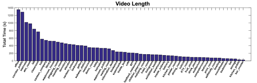
Figure 9: Distribution of scene categories in ISIA RGB-D.

VI ISIA RGB-D Video Database

In order to investigate scene recognition in RGB-D videos, we introduce the ISIA RGB-D video database. It contains indoor videos captured from three different cities (separated up to 1000 km), guaranteeing diversity in locations and scenes. The database reuses 58 of the categories in the taxonomy of the MIT indoor scene database [4], and has a total of 278 videos, with more than five hours of footage in total. The duration of the footage per category is shown in Fig. 9. The duration of videos varies, depending on the complexity and extension of the scene itself (a classroom or furniture store requires more footage than office or bedroom) and how common and easy to access are certain categories (e.g., office and classroom have more videos than auditorium or bowling alley). Videos are captured using a Microsoft Kinect version 2 sensor, with a frame rate of 15 frames/s, obtaining more than 275000 frames.

The database aims at addressing the limitations of the narrow field of view in conventional RGB-D sensors and the limited range of the depth one, by increasing the coverage by recording videos instead of images. In particular, it targets wide scenes, which we capture by starting on one side and moving to the other across the scene while panning the camera to maximize the coverage. Fig. 8 shows an example of the category classroom). Note that regions like the podium, the whiteboard and the windows are missing in the initial depth image, but are captured in other parts of the video sequence.

VII CNN-RNN Architecture for Video Recognition

Scene recognition with video data requires aggregating spatial features along time into a joint spatiotemporal representation. We propose a framework combining convolutional and recurrent neural networks that would capture spatial and temporal information, respectively, in a joint embedding (see Fig. 10). Particularly, the recurrent neural networks are implemented using Long-Short Term Memory (LSTM) units.

Similar to other works, our framework has independent branches for RGB and depth data, following the architecture for images. Temporal embedding with LSTMs is also modality-specific, and then late fusion is performed at sequence level using a fully connected layer. The combined architecture is trained jointly end-to-end.

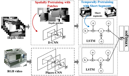
Figure 10: Framework of RGB-D video recognition.

VII-A Depth feature learning using pretraining with patches

As in RGB-D images, we face the problem of limited data to learn good neural representations from scratch, specially for depth data. We use the two-step training strategy described previously to learn depth features from limited data, in this case applied to both spatial and temporal dimensions. For the CNN we use patches and for the RNN we use short segments of frames, in both cases supervised by the scene label assigned to the whole video.

We sample the video and resize the keyframes to $256\times 256$ pixels. Following a similar strategy, we first pretrain the depth CNN model using patches. In the case of videos, patches are sampled from keyframes, and therefore are not limited to one image but to a segment or the whole sequence.

The pretrained model is then fine tuned with individual keyframes with stronger supervision. The fine tuned model can separately predict the scene probability for each frame.

VII-B Integrating temporal information

We use two strategies to integrate temporal information: average pooling and LSTM. The former is deterministic and used as baseline for comparison. We simply average the scene probabilities (i.e., output of the softmax of the image model) of all the keyframes. The latter exploits recurrent relations between keyframes by learning an LSTM embedding.

VII-C Training the temporal embedding

In contrast to averaging, the LSTM embedding needs to be trained. Since we have a limited number of sequences and keyframes, we follow a similar pretraining strategy using short segments of keyframes. In this case we apply it to both RGB and depth branches separately.

For each video, we sample sets of short segments. All these short segments have the same length of $T$ keyframes, from which modality-specific CNN features $X=[x_{1},x_{2},\ldots,x_{T}]$ are extracted. The core of the LSTM architecture is the memory cell $c$, which stores knowledge at each iteration according to the observed inputs and the current state. The behavior of the cell is determined by three different gates (input gate $i$, forget gate $f$, and output gate $o$) and several gating, update and output operations

$$i_{t} = \sigma\,(W_{ix}x_{t}+\,W_{im}m_{t-1}),$$ (1)

$$f_{t} = \sigma\,(W_{fx}x_{t}+\,W_{fm}m_{t-1}),$$ (2)

$$o_{t} = \sigma\,(W_{ox}x_{t}+\,W_{om}m_{t-1}),$$ (3)

$$c_{t} = f_{t}\,\odot c_{t-1}+i_{t}\odot h(W_{cx}x_{t}+\,W_{cm}m_{t-1}),$$ (4)

$$m_{t} = o_{t}\,\odot c_{t},$$ (5)

where $\sigma(\cdot)$ is the sigmoid function, $\odot(\cdot)$ represents the product with a gate value, and $h(\cdot)$ denotes the hyperbolic tangent function. The variable $m_{t}$ is the hidden state, $x_{t}$ is the input (CNN feature of each frame) of each step and the different $W$ are the weight matrices of the model.

VII-D RGB-D Fusion

Once the modality-specific branches are pretrained, we fine tune the joint model with the full videos. Note that, as in the case of images, the depth CNN is pretrained with patches while the RGB CNN is pretrained using a Places-CNN.

Although the predictions for RGB and depth can also be averaged, we find that it is more effective to combine them using a fully connected layer. This also allows us to train the model end-to-end.

VIII Experiments

VIII-A Settings

VIII-A1 Datasets

We first evaluate scene recognition on images, comparing the proposed D-CNN and RGB-D CNN models in two RGB-D datasets: NYUD2 [32] and SUN RGB-D [8]. The former is a relatively small dataset with 27 indoor categories, but only a few of them are well represented. Following the split in [32], all 27 categories are reorganized into 10 categories, including the 9 most common categories and an other category consisting of the remaining categories. The training/test split is 795/654 images. SUN RGB-D contains 40 categories with 10335 RGB-D images. Following the publicly available split in [8, 9], the 19 most common categories are selected, consisting of 4,845 images for training and 4,659 images for test.

We also evaluate the proposed video recognition method on the ISIA RGB-D video database. Eight scene categories contain only one video, so we use the other 50 categories (each of them with different numbers of videos, see Fig. 9). We randomly select nearly 60% of the data of each category for training, while the remaining are used for test. Following [8], we report the mean class accuracy for evaluations and comparisons.

VIII-A2 Classifier

Since we found that training linear SVM classifiers with the output of the fully connected layer increases performance slightly, all the following results are obtained including SVMs, unless specified otherwise.

• (wSVM): this variant uses category-specific weights during SVM training to compensate the imbalance in the training data. The weight $w=\{w_{1}...w_{K}\}$ of each category $k$ is computed as $w_{k}=\left(\frac{\min_{i\in K}N_{i}}{N_{k}}\right)^{p}$, where $N_{k}$ is the number of training images of the $k_{th}$ category. We selected $p=2$ empirically by cross-validation in a preliminary experiment.

VIII-A3 Evaluation metric

Following [8, 9], we report the average precision over all scene classes for all datasets.

VIII-B SUN RGB-D

VIII-B1 Depth features

We first compare D-CNN and Alex-CNN on the depth data of SUN RGB-D. The outputs of the different layers are used as features to train the SVM classifiers. Table I compares five different models. In Alex-CNN, we use all the layers of Places-CNN to initialize the network and then fine tune it, but only the three bottom convolutional layers when we train it from scratch, since the performance is higher than with the full architecture (see Fig.4).

The features extracted from the bottom layers (pool1 to conv3) trained from scratch obtain better performance for classification than those transferred from Places-CNN and fine tuned, even though for the top layers is worse. Using weakly-supervised training on patches (WSP), the performance increase is comparable to that of the top layer of the fine tuned Places-CNN and better than that of bottom layers, despite having fewer layers and not relying on Places data. D-CNN consistently achieves the best performance, despite being a smaller model.

TABLE I: Ablation study for different depth models. Accuracy (%) on SUN RGB-D.

Arch.	Alex-CNN				D-CNN
Weights	Places-CNN		Scratch		Scratch
	No FT	FT	No WSP	WSP	WSP
Layer
pool1	17.2	20.3	22.3	23.5	25.3
pool2	25.3	27.5	26.8	30.4	33.9
conv3	27.6	29.3	29.8	35.1	34.6
conv4	29.5	32.1	-	-	38.3
pool5	30.5	35.9	-	-	-
fc6	30.8	36.5	30.7	36.1	-
fc7	30.9	37.2	32.0	36.8	40.5
fc8	-	37.8	32.8	37.5	41.2

We also compare to related works using only depth features (see Table II). For a fair comparison, we also implemented SPP for Places-CNN. D-CNN outperforms FT-Places-CNN+SPP by 3.5%. Using the weighted SVM both models further improve more than 1%.

TABLE II: Accuracy on SUN RGB-D with depth features (%)

	Method	Acc.(%)
Proposed	D-CNN	41.2
	D-CNN (wSVM)	42.4
State-of-the-art	R-CNN+FV[9]	34.6
	FT-PL[9]	37.5
	FT-PL+SPP	37.7
	FT-PL+SPP (wSVM)	38.9
FT: Fine tuned, PL: Places-CNN

Figure 11: Impact of video length on modality-specific recognition on ISIA RGB-D.

TABLE III: Evaluation of object detection with depth data on SUN RGB-D in mAP (%)

Architecture	Init.	mAP (%)
ZF-net [42]	Scratch	29.3
ZF-net [42]	RGB-ZF-net	35.8
D-CNN	Scratch	34.6
D-CNN	WSP	38.1

In addition to scene recognition, we adapted the D-CNN model for object detection. We first pretrained the CNN model with patches sampled from depth images, which is then fine tuned with object annotations with the framework of Faster R-CNN [43]. Thus, D-CNN is used to initialize the convolutional layers of Faster R-CNN for object detection with depth data. Particularly for object detection, we use object annotations (provided by SUN RGB-D) to sample patches inside the bounding boxes of objects. The results are shown in Figs 12. This shows that the proposed D-CNN model with patch-level pretraining can also learn effective depth features for object detection, even outperforming a fine tuned RGB model (3.3% higher mAP than ZF-net).

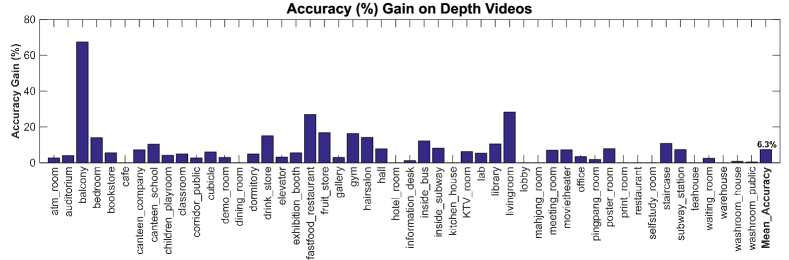
Figure 12: Accuracy (%) gain of using depth video data compared to image data.

TABLE IV: Accuracy (%) on SUN RGB-D

	Method	CNN models		Accuracy (%)
		RGB	Depth	RGB	Depth	RGB-D
Baseline	Concate.	PL	PL	35.4	30.9	39.1
	Concate.	FT-PL	FT-PL	41.5	37.5	45.4
	Concate. (wSVM)	FT-PL	FT-PL	42.7	38.7	46.9
	Concate.	R-CNN	R-CNN	44.6	41.4	47.8
Proposed	Concate.	FT-PL	FT-WSP-ALEX	-	37.5	48.5
	RGB-D-CNN	FT-PL	D-CNN	-	41.2	50.9
	RGB-D-CNN (wSVM)	FT-PL	D-CNN	-	42.4	52.4
	RGB-D-MS (wSVM)	FT-PL	D-CNN	-	-	53.4
	RGB-D-OB (wSVM)	FT-PL+ R-CNN	D-CNN + R-CNN	-	-	53.8
State-of-the-art	Zhu et al. [10]	FT-PL	FT-PL	40.4	36.5	41.5
	Wang et al. [9]	FT-PL+ R-CNN	FT-PL+ R-CNN	40.4	36.5	48.1
	Song et al. [44]	FT-PL	FT-PL+ ALEX	41.5	40.1	52.3
FT: Fine tuned, PL: Places-CNN

TABLE V: Accuracy (%) on NYUD2

	Features		Acc.
Method	RGB	Depth
Baseline methods
RGB	FT-PL	-	53.4
Depth	-	FT-PL	51.8
Concate.	FT-PL	FT-PL	59.5
RGB	R-CNN	-	52.2
Depth	-	R-CNN	48.9
Proposed methods
D-CNN	-	D-CNN	56.4
RGB-D-CNN	FT-PL	D-CNN	65.1
RGB-D-CNN (wSVM)	FT-PL	D-CNN	65.8
RGB-D-MS (wSVM)	FT-PL	D-CNN	67.3
RGB-D-OB (wSVM)	FT-PL	D-CNN	67.5
State-of-the-art
Gupta et al. [15]			45.4
Wang et al. [9]			63.9
Song et al. [44]			66.7
FT: Fine tuned, PL: Places-CNN

VIII-B2 RGB-D fusion

We compare with the performance of RGB-specific, depth-specific and combined RGB-D models. RGB-D models outperform the modality-specific ones, as expected (see Table IV). Places-CNN fine tuned on RGB still outperforms D-CNN, but just by 0.3%, showing the potential of depth features for scene recognition and the proposed training method. Furthermore, note that the accuracy of D-CNN on depth data not only outperforms significantly the fine tuned Places-CNN (by 3.7%), but this gain is even higher when combined with RGB in the multimodal case (by 5.5%). This suggests that depth features should be learned directly from depth data with a suitable architecture and training method, and highlights the limitations of transferring RGB-specific features to depth, even when trained on a large dataset such as Places. The higher gain also suggests that depth features learned from scratch are more complementary to RGB ones than those transferred from Places-CNN.

It is also interesting to compare the gain with respect the strongest modality-specific network, in this case FT-Places-CNN for RGB (e.g., 42.7% with wSVM), and the final multimodal result adding either FT-Places-CNN (depth) or D-CNN (46.9% and 52.4%, respectively). The gain is moderate in the former (4.2%), but much higher in the latter (9.7%), which further supports that depth features from D-CNN are more complementary to RGB ones, than those transferred from RGB networks.

Compared with other state-of-the-art methods for RGB-D scene recognition [10, 9], our method also obtains significantly higher accuracy by making a more effective use of depth data. These methods rely on fine tuning Places-CNN on depth data, which we showed is not desirable because low-level filters remain RGB-specific. Zhu et al. [10] learn discriminative RGB-D fusion layers that help to exploit the redundancy at high layers by aligning RGB and depth representations. This high-level redundancy largely results from the fact that both RGB and depth branches derive from Places-CNN and its RGB-specific features. In contrast, we avoid this unnecessary redundancy in the first place by learning discriminative features for depth from the very beginning (i.e., bottom layers), which are complementary to RGB ones rather than redundant. Wang et al. [9] extract objects and scene features for both RGB, depth and surface normals. Despite of exploiting more modalities and being more expensive computationally (due to object detection), that framework suffers from the same limitation, and the gain in their late multimodal fusion phase is largely due that type of redundancy. Recently, Song et al. [44] achieved similar performance to ours, by combining three AlexNet networks, one of them learning directly from depth. However, compared to our framework, theirs has much more complex models, is inefficient and has a very complex feature fusion method.

Additionally we also evaluated other RGB-D fusion methods. RGB-D-MS (wSVM) represents a multi-scale RGB-D fusion variant inspired by [44], where we connect lower convolutional layers (such as conv2 and conv3 in Fig. 7) of D-CNN to the last fully connected layer with the same operations as in [44]. By combining the lower layers of D-CNN, RGB-D-MS outperforms previous RGB-D-CNN (which only concatenates the last fully connected layers of RGB and depth CNNs) by 1.0% in accuracy, and outperforms the state-of-the-art work [44] by 1.1%. The improvement of RGB-D-MS mainly benefits from the integrating the lower convolutional layers of D-CNN, which learns depth-specific patterns as shown in Fig. 5 (h). RGB-D-OB (wSVM) represents the fusion of RGB-D-CNN features and features extracted by object detection, which is inspired by [9]. In our implementation, RGB-D-OB combines four types of features: two global (i.e. fine tuned Places CNN with RGB and D-CNN) and two local extracted with Faster R-CNN [43] (i.e. from RGB and depth images, using the RGB ZF-net architecture [42] and the proposed D-CNN, respectively). With object based features, the RGB-D-OB (wSVM) variant outperforms [44] by 1.5%.

TABLE VI: Accuracy (%) on ISIA RGB-D (short videos).

	Method	Step 1	Step 2	Accuracy (%)
		RGB-D Fusion	Temporal Embedding	RGB	Depth	RGB-D
Baselines	CNN+AVE	-	AVE	42.9	34.9	-
	CNN+AVE	AVE	AVE	-	-	48.1
Other	CNN (RGB-D)+LSTM	Concatenation	LSTM	-	-	48.0
	Method	Step 1	Step 2	Accuracy (%)
		Temporal Embedding	RGB-D Fusion	RGB	Depth	RGB-D
Others	CNN+LSTM	LSTM	-	43.3	36.6	-
	CNN+LSTM	LSTM	Concatenation	-	-	48.7
Proposed	CNN+LSTM (EtE)	LSTM	-	44.9	38.3	-
	CNN+LSTM (EtE)	LSTM	Concatenation	-	-	49.9
EtE: end to end, AVE: average pooling

TABLE VII: Accuracy (%) on ISIA RGB-D (full length videos).

RGB-D	TE	Accuracy (%)
			RGB	Depth	RGB-D
CNN+AVE	-	AVE	52.8	47.2	-
CNN+AVE	AVE	AVE	-	-	56.5
Method	RGB-D	TE	Accuracy (%)
			RGB	Depth	RGB-D
CNN+LSTM (EtE)	-	LSTM	55.6	48.1	-
CNN+LSTM (EtE)	LSTM	Con.	-	-	58.3
TE: Temporal Embedding, Con.: Concatenation
EtE: End to End, AVE: Average Pooling

VIII-C NYUD2

We also evaluated our approach on NYUD2 and compared to other representative works (see Table V). Both methods use more complex frameworks including explicit scene analysis. Gupta et al. [15] rely on segmentation and handcrafted features, while Wang et al. on extracting object detection [9]. Despite these more structured representations, our approach also outperforms them. Handcrafted and transferred features are also more competitive when the training data is more limited. Despite NYUD2 has fewer training images, our method still can learn better depth and multimodal representations. Song et al. [44] achieve slightly better performance than ours with their three AlexNet framework.

We also extend our RGB-D-CNN model with the tricks of multi-scale fusion and integration with objected based features on NYUD2. The extended results on NYUD2 are shown in Table IV. Compared to [44], the proposed RGB-D-MS (wSVM) obtains a gain of 0.6%, and RGB-D-OB (wSVM) obtains a gain of 0.8%. It is more fair to compare RGB-D-OB (wSVM) with [9], since both works integrate global features (extracted from CNN model) and local features (extracted with object detection). RGB-D-OB (wSVM) outperforms [9] by a clear margin of 3.9%.

VIII-D ISIA RGB-D

We evaluated the proposed approach on videos, in order to study how accumulating temporal information helps recognition.

VIII-D1 Data preprocessing

One problem with the capture of RGB-D videos is that RGB frames are often blurry, and we found it affected the performance. In order to alleviate this problem, for our experiments we use a quasilinear sampling strategy in which we select the least blurred frame every segment of 5 frames (i.e., sampling approximately 3 frames/s). The degree of blur is measured as the mean value of the gradient between pixels (the larger, the less blurry).

Depth videos are stored in 8 bit gray scale. We encode depth frames to 3-channel images using jet color encoding. We chose this encoding in this case since it has been shown that the performance is comparable to HHA encoding while being much faster to compute [13].

VIII-D2 Impact of video length

The number of frames integrated in the recognition process is an important parameter. Thus, we first evaluate its impact on the recognition performance for RGB and depth modalities. We compare two methods to integrate temporal information: average pooling of the predictions obtained by the CNN network (AVE) and feeding frame CNN features to a LSTM network (LSTM). We further include a variant where both CNNs and LSTMs are trained end-to-end (EtE).

The results are shown in Fig. 11. While for RGB the gain is very marginal, for depth the gain is significantly higher and increasing with the number of frames. Since the range of RGB cameras is much larger than that of depth ones, the additional RGB frames do not provide much more additional information, in contrast to additional depth frames which contain new information that cannot be captured in each frame separately. This trend is observed in the three methods evaluated, with LSTM outperforming average pooling, in particular when using end-to-end training. Particularly, we also show the detailed comparisons between recognition with images (i.e., one frame videos) and videos with 18 frames in Fig. 12. Each bar in Fig. 12 indicate the gain of using videos, comparing to using images (one frame videos), for scene recognition with depth data. It can be observed that mAP (%) of most object categories are improved when recognizing with videos with multiple frames. The clear margin of average gain (about 6.3% in mAP) illustrates the efficiency of recognizing scenes with depth video data.

VIII-D3 RGB-D recognition

We evaluated the different variants on both short and full length videos. For the former, from each video we sample several short segments, resulting in more training samples but with fewer frames each. We compared different variants where the order of RGB-D fusions and temporal integration (i.e., temporal embedding) are different.

The short videos are basically segments of 9 key frames sampled from the full length videos. The results are shown in Table VI. As in previous datasets, the RGB network has higher performance than the depth network. Average pooling is outperformed by LSTM based methods, with end-to-end training helping more. The order of temporal embedding and fusion is important, and in our experiments the best results are obtained when the temporal embedding is performed before the RGB-D fusion. Interestingly, end-to-end fine tuning decreases slightly the accuracy of RGB only recognition, while increasing significantly that of depth and RGB-D.

The evaluation on long videos is shown in Table VII. The results are very similar, with the best result obtained by combining both modalities after modality-specific temporal embedding and end-to-end training. Accuracies are higher than in the case of short videos because the network can integrate more temporal information during both training and inference.

IX Conclusion

Compared to RGB, learning genuine depth features is challenging due to the limited data available and the limited information captured by the limited range of depth sensors. This problem is usually tackled using transfer learning, from a deep RGB network trained on a large dataset (e.g., Places) and then fine tuning with the target depth data. While effective for the RGB modality, it has significant limitations for depth data that we highlight in this work. The most important is that low level filters remain RGB-specific and cannot capture depth-specific patterns.

We use a radically different approach by focusing mainly on learning good low level depth-specific filters. A smaller architecture and a weakly supervised pretraining strategy for the bottom layers enables us to overcome the problem of very limited depth data. In this way, the network captures patterns that fine tuned RGB networks are not able to, and these patterns will be more complementary to RGB ones in the joint RGB-D network.

Integrating temporal information is particularly helpful for depth data, capturing in this way information about both near and distant objects. This is not possible in just one image with current depth sensors. We studied this case in a new multimodal video scene recognition dataset.

In general, our results show that the proposed training strategy and spatio-temporal model can exploit much better the depth modality, with a significantly higher gain over RGB-only scene recognition than in previous works. We hope this work and dataset can motivate further research in these directions.

References

- [1] B. Zhou, A. Lapedriza, J. Xiao, A. Torralba, and A. Oliva, “Learning deep features for scene recognition using places database,” in Advances in Neural Information Processing Systems (NIPS), 2014, pp. 487–495.
- [2] A. Krizhevsky, I. Sutskever, and G. E. Hinton, “Imagenet classification with deep convolutional neural networks,” in Advances in Neural Information Processing Systems (NIPS), 2012, pp. 1106–1114.
- [3] K. Simonyan and A. Zisserman, “Very deep convolutional networks for large-scale image recognition,” in International Conference on Learning Representations (ICLR), 2015.
- [4] A. Quattoni and A. Torralba, “Recognizing indoor scenes,” in IEEE Conference on Computer Vision and Pattern Recognition (CVPR), 2009.
- [5] J. Xiao, J. Hayes, K. Ehringer, A. Olivia, and A. Torralba, “SUN database: Largescale scene recognition from abbey to zoo,” in IEEE Conference on Computer Vision and Pattern Recognition (CVPR), 2010.
- [6] J. Donahue, Y. Jia, O. Vinyals, J. Hoffman, N. Zhang, E. Tzeng, and T. Darrell, “DeCAF: A deep convolutional activation feature for generic visual recognition,” in International Conference on Machine Learning (ICML), 2014.
- [7] N. Silberman and R. Fergus, “Indoor scene segmentation using a structured light sensor,” in International Conference on Computer Vision (ICCV) Workshops, Nov. 2011, pp. 601–608.
- [8] S. Song, S. P. Lichtenberg, and J. Xiao, “SUN RGB-D: A RGB-D scene understanding benchmark suite,” in IEEE Conference on Computer Vision and Pattern Recognition (CVPR), Jun. 2015, pp. 567–576.
- [9] A. Wang, J. Cai, J. Lu, and T.-J. Cham, “Modality and component aware feature fusion for RGB-D scene classification,” in IEEE Conference on Computer Vision and Pattern Recognition (CVPR), June 2016.
- [10] H. Zhu, J.-B. Weibel, and S. Lu, “Discriminative multi-modal feature fusion for RGBD indoor scene recognition,” in IEEE Conference on Computer Vision and Pattern Recognition (CVPR), June 2016.
- [11] S. Gupta, J. Hoffman, and J. Malik, “Cross modal distillation for supervision transfer,” in IEEE Conference on Computer Vision and Pattern Recognition (CVPR), June 2016.
- [12] Z. Wang, R. Lin, J. Lu, J. Feng et al., “Correlated and individual multi-modal deep learning for rgb-d object recognition,” arXiv preprint, 2016.
- [13] A. Eitel, J. T. Springenberg, L. Spinello, M. Riedmiller, and W. Burgard, “Multimodal deep learning for robust RGB-D object recognition,” in International Conference on Intelligent Robots and Systems (IROS), 2015, pp. 681–687.
- [14] X. Song, L. Herranz, and S. Jiang, “Depth CNNs for RGB-D scene recognition: Learning from scratch better than transferring from rgb-cnns,” in AAAI Conference on Artificial Intelligence, 2017, pp. 4271–4277.
- [15] S. Gupta, P. Arbeláez, R. Girshick, and J. Malik, “Indoor scene understanding with RGB-D images: Bottom-up segmentation, object detection and semantic segmentation,” International Journal of Computer Vision, vol. 112, no. 2, pp. 133–149, 2015.
- [16] D. Banica and C. Sminchisescu, “Second-order constrained parametric proposals and sequential search-based structured prediction for semantic segmentation in rgb-d images,” in IEEE Conference on Computer Vision and Pattern Recognition (CVPR), June 2015.
- [17] R. Socher, B. Huval, B. Bath, C. D. Manning, and A. Y. Ng, “Convolutional-recursive deep learning for 3D object classification,” in Advances in Neural Information Processing Systems (NIPS), 2012.
- [18] S. Gupta, R. Girshick, P. Arbelaez, and J. Malik, “Learning rich features from RGB-D images for object detection and segmentation,” in European Conference on Computer Vision (ECCV), 2014.
- [19] T. Durand, N. Thome, and M. Cord, “WELDON: Weakly supervised learning of deep convolutional neural networks,” in IEEE Conference on Computer Vision and Pattern Recognition (CVPR), June 2016.
- [20] H. Bilen and A. Vedaldi, “Weakly supervised deep detection networks,” in IEEE Conference on Computer Vision and Pattern Recognition (CVPR), June 2016.
- [21] M. Oquab, L. Bottou, I. Laptev, and J. Sivic, “Is object localization for free? - weakly-supervised learning with convolutional neural networks,” in IEEE Conference on Computer Vision and Pattern Recognition (CVPR), June 2015.
- [22] N. Rasiwasia and N. Vasconcelos, “Holistic context modeling using semantic co-occurrences,” in IEEE Conference on Computer Vision and Pattern Recognition (CVPR), 2009, pp. 1889–1895.
- [23] ——, “Holistic context models for visual recognition,” IEEE Transactions on Pattern Analysis and Machine Intelligence, vol. 34, no. 5, pp. 902–917, 2012.
- [24] X. Song, S. Jiang, and L. Herranz, “Joint multi-feature spatial context for scene recognition on the semantic manifold,” in IEEE Conference on Computer Vision and Pattern Recognition (CVPR), June 2015.
- [25] X. Song, S. Jiang, L. Herranz, Y. Kong, and K. Zheng, “Category co-occurrence modeling for large scale scene recognition,” Pattern Recognition, vol. 59, pp. 98 – 111, 2016.
- [26] Z. Wang, L. Wang, Y. Wang, B. Zhang, and Y. Qiao, “Weakly supervised patchnets: Describing and aggregating local patches for scene recognition,” IEEE Transactions on Image Processing, vol. 26, no. 4, pp. 2028–2041, 2017.
- [27] X. Song, S. Jiang, and L. Herranz, “Multi-scale multi-feature context modeling for scene recognition in the semantic manifold,” IEEE Transactions on Image Processing, vol. 26, no. 6, pp. 2721–2735, 2017.
- [28] C. Feichtenhofer, A. Pinz, and R. P. Wildes, “Temporal residual networks for dynamic scene recognition,” in IEEE Conference on Computer Vision and Pattern Recognition (CVPR), July 2017.
- [29] K. G. Derpanis, M. Lecce, K. Daniilidis, and R. P. Wildes, “Dynamic scene understanding: The role of orientation features in space and time in scene classification,” in IEEE Conference on Computer Vision and Pattern Recognition (CVPR), 2012.
- [30] N. Shroff, P. Turaga, and R. Chellappa, “Moving vistas: Exploiting motion for describing scenes,” in IEEE Conference on Computer Vision and Pattern Recognition (CVPR), June 2010, pp. 1911–1918.
- [31] J. Xiao, A. Owens, and A. Torralba, “Sun3d: A database of big spaces reconstructed using sfm and object labels,” in International Conference on Computer Vision (ICCV), 2013, pp. 1625–1632.
- [32] N. Silberman, D. Hoiem, P. Kohli, and R. Fergus, “Indoor segmentation and support inference from RGBD images,” in European Conference on Computer Vision (ECCV), ser. ECCV’12, 2012, pp. 746–760.
- [33] A. Karpathy, G. Toderici, S. Shetty, T. Leung, R. Sukthankar, and L. Fei-Fei, “Large-scale video classification with convolutional neural networks,” in IEEE Conference on Computer Vision and Pattern Recognition (CVPR), June 2014, pp. 1725–1732.
- [34] K. Simonyan and A. Zisserman, “Two-stream convolutional networks for action recognition in videos,” in Advances in Neural Information Processing Systems (NIPS), Z. Ghahramani, M. Welling, C. Cortes, N. D. Lawrence, and K. Q. Weinberger, Eds., 2014, pp. 568–576.
- [35] C. Feichtenhofer, A. Pinz, and A. Zisserman, “Convolutional two-stream network fusion for video action recognition,” in IEEE Conference on Computer Vision and Pattern Recognition (CVPR), June 2016.
- [36] K. He, X. Zhang, S. Ren, and J. Sun, “Deep residual learning for image recognition,” in IEEE Conference on Computer Vision and Pattern Recognition (CVPR), June 2016.
- [37] S. Lazebnik, C. Schmid, and J. Ponce, “Beyond bags of features: Spatial pyramid matching for recognizing natural scene categories,” in IEEE Conference on Computer Vision and Pattern Recognition (CVPR), 2006.
- [38] P. Agrawal, R. Girshick, and J. Malik, “Analyzing the performance of multilayer neural networks for object recognition,” in European Conference on Computer Vision (ECCV). Springer, 2014, pp. 329–344.
- [39] X. Song, S. Jiang, and L. Herranz, “Joint multi-feature spatial context for scene recognition on the semantic manifold,” in IEEE Conference on Computer Vision and Pattern Recognition (CVPR), 2015, pp. 1312–1320.
- [40] K. He, X. Zhang, S. Ren, and J. Sun, “Spatial pyramid pooling in deep convolutional networks for visual recognition,” in European Conference on Computer Vision (ECCV), 2014.
- [41] A. Wang, J. Lu, J. Cai, T.-J. Cham, and G. Wang, “Large-margin multi-modal deep learning for rgb-d object recognition,” IEEE Transactions on Multimedia, vol. 17, 2015.
- [42] M. D. Zeiler and R. Fergus, “Visualizing and understanding convolutional networks,” in European Conference on Computer Vision (ECCV), Cham, 2014, pp. 818–833.
- [43] S. Ren, K. He, R. Girshick, and J. Sun, “Faster R-CNN: Towards real-time object detection with region proposal networks,” in Advances in Neural Information Processing Systems (NIPS), C. Cortes, N. D. Lawrence, D. D. Lee, M. Sugiyama, and R. Garnett, Eds., 2015, pp. 91–99.
- [44] X. Song, S. Jiang, and L. Herranz, “Combining models from multiple sources for RGB-D scene recognition,” in International Joint Conference on Artificial Intelligence (IJCAI), 2017, pp. 4523–4529.