Enhanced high-order harmonic generation in donor-doped band-gap materials

Abstract

We find that a donor-doped band-gap material can enhance the overall high-order harmonic generation (HHG) efficiency by several orders of magnitude, compared with undoped and acceptor-doped materials. This significant enhancement, predicted by time-dependent density functional theory simulations, originates from the highest occupied impurity state which has an isolated energy located within the band gap. The impurity-state HHG is rationalized by a three-step model, taking into account that the impurity-state electron tunnels into the conduction band and then moves according to its band structure until recombination. In addition to the improvement of the HHG efficiency, the donor-type doping results in a harmonic cutoff different from that in the undoped and acceptor-doped cases, explained by semiclassical analysis for the impurity-state HHG.

I Introduction

High-order harmonic generation (HHG) in gases Krause et al. (1992); L’Huillier and Balcou (1993) is not only one of the fundamental strong-field phenomena in laser-matter interactions. It is also a powerful technique to produce sub-femtosecond laser pulses, providing the opportunity to explore ultrafast dynamics in matter on femto- and attosecond timescales Krausz and Ivanov (2009). Recently, HHG in solids was demonstrated Ghimire et al. (2011); Schubert et al. (2014); Luu et al. (2015); Vampa et al. (2015a); Hohenleutner et al. (2015); Ndabashimiye et al. (2016) with potential applications for novel VUV and XUV light sources and for probing ultrafast dynamics in condensed-matter systems Kruchinin et al. (2018). Compared with gas-phase systems, solids can possibly produce HHG more efficiently due to their periodic structure and high density. Also, laser-induced processes in bulk and nanostructured materials attract theoretical interests in this new research area where strong-field laser physics meets condensed matter. It has been demonstrated that some strong-field concepts, such as the three-step model for HHG Corkum (1993), can be generalized to describe laser-solid interactions when the band structure is taken into account Vampa et al. (2014); Vampa and Brabec (2017). Although the understanding of HHG in solids is rapidly expanding Higuchi et al. (2014); Vampa et al. (2014); Vampa and Brabec (2017); Vampa et al. (2015b); McDonald et al. (2015); Hawkins et al. (2015); Wu et al. (2015, 2016); Guan et al. (2016); Du et al. (2018a, b); Jin et al. (2018); Luu and Wörner (2016); Földi (2017); Osika et al. (2017); Tancogne-Dejean et al. (2017); Hansen et al. (2017, 2018); Bauer and Hansen (2018); Murakami et al. (2018); Silva et al. (2018); Luu and Wörner (2018), many open questions remain to be explored.

For applications of HHG in solids as a coherent VUV or XUV source, a key question is how to control the harmonic yield. A recent experiment has demonstrated enhanced HHG emission in tailored semiconductors Sivis et al. (2017). Theoretical studies have proposed possibilities to enhance HHG in solids by quantum confinement McDonald et al. (2017), inhomogeneous fields Du et al. (2016), or substitutional doping Huang et al. (2017). Indeed, impurities typically influence the physical properties of a solid, allowing one to control processes in the target material for various applications (see, e.g., the recent works Burgess et al. (2016); Klyukin et al. (2018)). Doping-induced impurities are therefore expected to have impact on HHG in solids. The specific influence of doping-induced impurities, however, still requires further exploration, even in the case of substitutional doping . Here, to elucidate effects of substitutional doping on HHG in solids, we consider a model of undoped and doped band-gap materials interacting with a mid-infrared laser pulse, use time-dependent density functional theory (TDDFT) Runge and Gross (1984); Ullrich (2011) to perform self-consistent calculations, and provide a semiclassical analysis for the impurity-state HHG cutoff.

This paper is organized as follows. In Sec. II, we describe the theoretical model and methods used in this work. The results of our theoretical calculations are presented and discussed in Sec. III. Finally we conclude with a brief summary in Sec. IV. Atomic units (a.u.) are used throughout unless stated otherwise.

II Theoretical Model and Methods

Our model employs a finite system so large that it behaves like a solid Hansen et al. (2017, 2018); Bauer and Hansen (2018). We consider a linear chain of $N$ nuclei with a separation $a$ and located at $x_{j}=[j-(N+1)/2]a$, ($j=1,\cdots,N$). The ionic potential reads $v_{\text{ion}}(x)=-\sum_{j=1}^{N}Z_{j}[(x-x_{j})^{2}+\epsilon]^{-1/2}$, where $Z_{j}$ is the nuclear charge of the $j$-th ion and $\epsilon$ is a softening parameter which smoothens the Coulomb singularity. We set $\epsilon=2.25$ and $a=7$ throughout, and use $Z_{j}=4$ ($j=1,\cdots,N$) to qualitatively model an undoped band-gap material. For a convenient description of substitutional doping, we choose an odd number of nuclei ($N=2M-1=101$ in this work) and introduce an impurity in the center by choosing a different nuclear charge of the $M$-th ion. As we will see below, such a doping rate of $\sim 1\%$ does not change the band structures significantly, but introduces new states that are energetically isolated. Also, our discussion of doping effects is insensitive to the model size, once a sufficiently large number of nuclei ($\gtrsim 80$) is considered (see the Appendix). In our simulations, two doping cases are considered: $Z_{M}=2$ for modeling a double acceptor and $Z_{M}=6$ for modeling a double donor Pantelides (1978). All the considered systems are charge and spin neutral. Thus the number of electrons with opposite spin is $N_{\downarrow}=N_{\uparrow}=2N$ for the undoped case, and $N_{\downarrow}=N_{\uparrow}=2N\pm 1$ for the systems with a doped center ($Z_{M}=4\pm 2$). We treat the field-free electronic states for these systems with density functional theory (DFT). In the Kohn-Sham (KS) scheme, we find a set of KS orbitals determined by

$$\left\{-\frac{1}{2}\frac{\partial^{2}}{\partial x^{2}}+v_{\text{KS}}[\{n_{\sigma}\}](x)\right\}\varphi_{j,\sigma}(x)=\varepsilon_{j,\sigma}\varphi_{j,\sigma}(x),$$ (1)

with the static KS potential $v_{\text{KS}}[\{n_{\sigma}\}](x)=v_{\text{ion}}(x)+v_{\text{H}}[n](x)+v_{\text{xc}}[\{n_{\sigma}\}](x)$. The Hartree potential reads $v_{\text{H}}[n](x)=\int{dx^{\prime}}n(x^{\prime})[(x-x^{\prime})^{2}+\epsilon]^{-1/2}$, and the exchange-correlation potential is treated in a local spin-density approximation $v_{\text{xc}}[{n_{\sigma}}](x)\simeq v_{\text{x}}[{n_{\sigma}}](x)=-[6n_{\sigma}(x)/\pi]^{1/3}$. The spin densities are $n_{\sigma}(x)=\sum_{j=1}^{N_{\sigma}}|\varphi_{j,\sigma}(x)|^{2}$ for spin $\sigma={\downarrow,\uparrow}$, and the total density is $n(x)=\sum_{\sigma=\downarrow,\uparrow}n_{\sigma}(x)$.

For the driving laser pulse linearly polarized along the $x$-axis, we use the vector potential $A(t)=A_{0}\sin^{2}[\omega_{0}t/(2N_{c})]\sin(\omega_{0}t)$ for $0\leq{t}\leq 2\pi{N_{c}}/\omega_{0}$, with $\omega_{0}$ the angular frequency (photon energy) and $N_{c}$ the number of cycles. The laser-driven many-electron system is governed by the time-dependent KS equations

$$i\frac{\partial}{\partial t}\varphi_{j,\sigma}(x,t)$$

$$=\left\{-\frac{1}{2}\frac{\partial^{2}}{\partial x^{2}}-iA(t)\frac{\partial}{\partial x}+\tilde{v}_{\text{KS}}[\{n_{\sigma}\}](x,t)\right\}\varphi_{j,\sigma}(x,t),$$ (2)

where the KS potential $\tilde{v}_{\text{KS}}[\{n_{\sigma}\}](x,t)=v_{\text{ion}}(x)+v_{\text{H}}[n](x,t)+v_{\text{xc}}[\{n_{\sigma}\}](x,t)$ is time-dependent due to the time dependence of $n(x,t)$ and $n_{\sigma}(x,t)$. We propagate the time-dependent KS orbitals using the Crank-Nicolson approach with a predictor-corrector step for updating the KS potential Bauer (2017); Ullrich (2011). The initial conditions for TDDFT calculations, i.e., the field-free ground-state KS orbitals are found via imaginary time propagation with orthogonalization in each time step Bauer (2017). The numerical calculations are performed on an equidistant spatial grid with spacing $\Delta x=0.1$ and $21000$ grid points. A fixed step size $\Delta t=0.1$ is used for time propagation, and a convergence check is performed by using $\Delta t=0.05$.

III Results and Discussion

In this section, we first describe the influence of doping on the field-free potentials, orbital energies and band structures within the KS scheme. Then we discuss effects of doping on the HHG spectrum based on the TDDFT calculations, and identify the contribution from a single impurity orbital in the donor-doped case. Finally, the HHG cutoff is explained by semiclassical analysis.

III.1 Doping effects in the DFT description

We first take a view on the doping-induced change of the field-free properties in the DFT language. The undoped model was studied in Refs. Hansen et al. (2017, 2018). Here we first emphasize the differences between the doped and undoped systems in terms of the static KS potential which is obtained by imaginary time propagation. The impact of the impurity is restricted in real space to a small region around its position, the center of the system in this case, as shown in Fig. 1(a). Compared with the undoped system, the acceptor- and donor-type doping results in a shallower and deeper effective potential around the impurity ion, respectively. Unlike the single-active-electron approach using a parametrized potential Huang et al. (2017), the effective potential in the DFT description is self-consistently found in a many-electron model.

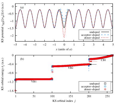
Figure 1: Comparisons of undoped and doped systems in the KS scheme. (a) The KS potentials around the impurity for the undoped and doped systems. The separation between two neighboring ions is $a=7$ in our model. (b) The negative-valued KS orbital energies in ascending order, including two valence bands (VB1 and VB2) and part of a conduction band (CB1). For the undoped, acceptor-doped and donor-doped systems, the number of occupied orbitals is $N_{\downarrow}=N_{\uparrow}=202$, $201$ and $203$, respectively (indicated by solid black, dashed blue and dotted red lines with arrows). In the doped cases, isolated orbital energies appear, which cannot be classified into any band.

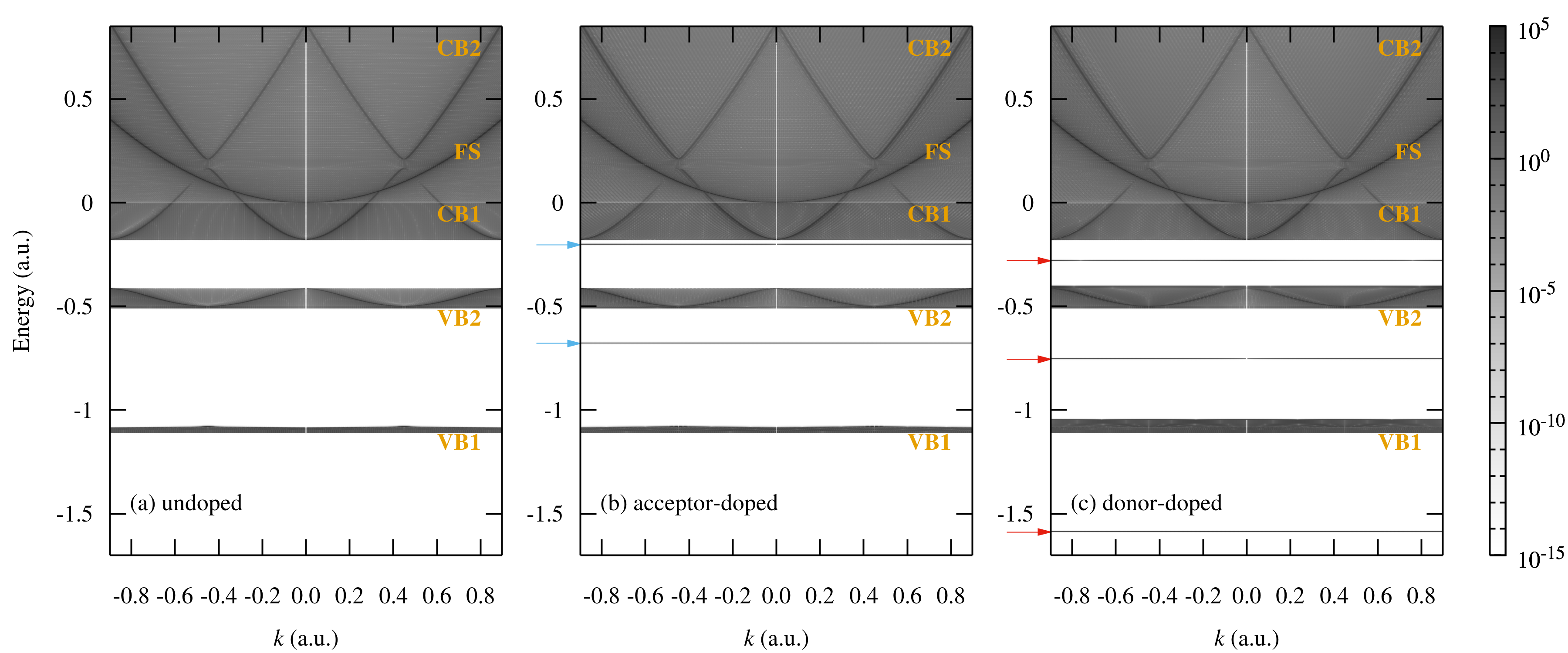
Figure 2: Band structures (VB1, VB2, CB1 and CB2) for undoped and doped systems with $N=101$ nuclei, displayed by norm square of the Fourier-transformed KS orbitals. The free-space (FS) dispersion $k^{2}/2$ is also visable due to the finiteness of the simulation box (see text). In the doped cases, the isolated horizontal lines correspond to impurity orbitals, which are also indicated by arrows. The first-Brillouin-zone boundary is at $k=\pi/a=0.449$.

With the static KS potential at hand, one can find the occupied and unoccupied orbitals by diagonalization, together with their corresponding energies. Note that in the KS scheme, the classification into occupied and unoccupied orbitals is automatically determined by the number of electrons with the Pauli exclusion principle satisfied, which is another advantage over the frequently-used single-active-electron approach (see, e.g., Refs. Hawkins et al. (2015); Wu et al. (2015, 2016); Guan et al. (2016); Du et al. (2016, 2018a, 2018b); Huang et al. (2017); Jin et al. (2018)). To illustrate the doping effects on the KS orbitals, we present in Fig. 1(b) the negative-valued orbital energies in ascending order. The energies include two valence bands (VB1 and VB2) and part of a conduction band (CB1), and the “in-band” energies remain almost unchanged by doping. Here we classify the orbital energies into bands, since our model behaves like a solid for a sufficiently large system size Hansen et al. (2018). The visible band gap (BG) allows us to identify the doping-induced impurity orbitals with isolated energies. In addition to their isolated energies, the impurity orbitals are spatially localized around the impurity ion (see the Appendix). In the case of acceptor- (donor-) type doping, the impurity orbital energetically located between VB2 and CB1 is unoccupied (occupied). It is worth noting that the impurity KS orbitals can be seen as a self-consistent DFT description of the “impurity states” introduced in the pioneering works Slater (1949); Luttinger and Kohn (1955), see also reviews Kohn (1957); Bassani et al. (1974); Pantelides (1978). For our purpose of exploring doping effects on HHG, it is straightforward to perform self-consistent simulations without resorting to additional assumptions. Thus both “in-band” and impurity orbitals are taken into account, and one can investigate their respective contributions in the many-electron processes. Whether an impurity orbital (state) plays a particular role in HHG will be studied in Sec. III.3.

The band structures can be constructed from the Fourier-transformed orbitals (in $k$-space), as done in Refs. Hansen et al. (2017, 2018). Figure 2 shows the norm square of the $k$-space KS orbitals for the undoped and doped systems with $N=101$ nuclei. The energy range in this plot includes two valence bands (VB1 and VB2) and two conduction band (CB1 and CB2). Since our simulations are performed in a finite box, the free-space (FS) dispersion $k^{2}/2$ is also present in Fig. 2. For HHG in solids, however, the FS parabola does not play any noticeable role Hansen et al. (2017, 2018). We find that the band structures are almost not affected by doping, except that the energy range of VB1 becomes wider when the system is donor-doped. The role of VB1 in HHG processes, however, is negligible because of the flat band structure and the low orbital energies, which has been demonstrated in Ref. Hansen et al. (2017). Figure 2 clearly shows that the considered doping scenarios generate energetically isolated orbitals which do not belong to any band. One can identify two impurity orbitals from Fig. 2(b) in the acceptor-type doping case, and three impurity orbitals from Fig. 2(c) in the donor-type doping case. A detailed view of these impurity orbitals in real space is presented in the Appendix.

III.2 Doping effects on the HHG spectrum

Using the ground-state occupied KS orbitals as the initial state, we perform TDDFT calculations for the systems interacting with a $6$-cycle laser pulse of frequency $\omega_{0}=0.0114$ corresponding to a wavelength of $\sim 4000$ nm. We compute the time-dependent current

$$J(t)=\sum_{j,\sigma}\int dx\ \text{Re}\left[\varphi_{j,\sigma}^{*}(x,t)\left(-i\frac{\partial}{\partial x}+A(t)\right)\varphi_{j,\sigma}(x,t)\right],$$ (3)

and evaluate the HHG spectral intensity as the modulus square of the Fourier-transformed current, i.e., $S(\omega)\propto|\int{dt}J(t)\exp(-i{\omega}t)|^{2}$. Here we do not account for macroscopic propagation effects, which may modify the HHG spectra via absorption and phase mismatch. Such propagation effects, however, can be mitigated by controlling the thickness of target materials Ndabashimiye et al. (2016). Therefore we expect our conclusions to hold for a thin target material.

Figure 3(a) shows HHG spectra for the undoped and doped systems obtained from TDDFT calculations, for $A_{0}=0.22$ which corresponds to an intensity of $\sim 2.2\times 10^{11}$ W/cm². The BG between CB1 and VB2 is $0.235\sim 6.4$ eV typical for a dielectric, implying that harmonics up to order 20 are in the sub-BG regime for the undoped system. The spectral minimum in the sub-BG region stems from the fact that the intensity of intraband harmonics decreases with increasing order and the interband harmonics become dominant when going into the above-BG regime. The HHG spectrum for the acceptor-doped system is very similar to that for the undoped system. In contrast, the overall HHG for the donor-doped system is enhanced by $\sim 2-6$ orders of magnitude. This significant enhancement of the HHG efficiency would be favorable for applications as a coherent source of VUV and XUV radiation. We also perform calculations with a frozen ground-state KS potential. Such a frozen-KS-potential approach is applicable for moderate intensities well below the damage threshold of solids Hansen et al. (2017). The spectra obtained from these calculations are shown in Fig. 3(b). The considerable enhancement of HHG in the donor-type doping case and the similarity of the undoped and acceptor-doped cases are also found with this approach. As will be shown in Sec. III.3, the frozen-KS-potential approach offers the possibility to identify the contribution from a single impurity orbital, which provides insights into the observed enhancement of HHG in the donor-type doping case. In addition, a different cutoff for the donor-doped system is found in Fig. 3, which will be analyzed in Sec. III.4.

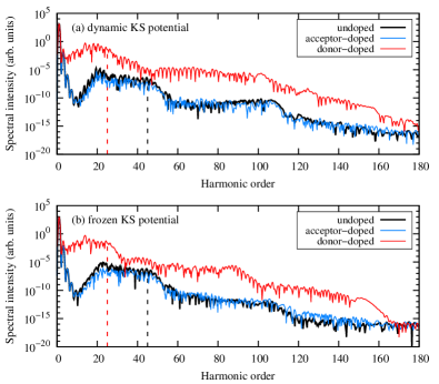
Figure 3: HHG spectra for undoped and doped systems obtained from (a) TDDFT calculations with the KS potential dynamically updated according to the time-dependent densities, and (b) calculations with the KS potential frozen to its field-free ground-state form. In both panels, the donor-doped system gives the highest yield. The laser parameters correspond to a wavelength of $\sim 4000$ nm and a peak intensity of $\sim 2.2\times 10^{11}$ W/cm² (see text). The vertical dashed lines indicate the first cutoffs: a cutoff of order 45 is observed for the undoped and acceptor-doped systems while a cutoff of order 25 is observed for the donor-doped system.

III.3 Role of a single impurity orbital

To understand the doping effects on HHG, we link our findings in Fig. 3 to the doping-induced changes of the field-free properties displayed in Fig. 1 and Fig. 2. Let us first revisit the intra- and interband contributions of HHG in undoped solids Vampa et al. (2014); Vampa and Brabec (2017). Intraband HHG stems from the laser-driven electron motion in bands due to the anharmonicity of the band structure. Interband HHG is described by the generalized three-step model for band-gap materials: first an electron tunnels into the conduction band, leaving a hole in the valence band; then the electron and hole move in their respective bands and may recombine at a later time, emitting a photon with energy above the BG. Thus the BG energy plays a similar role as the ionization potential in atomic HHG. If the energy of the highest occupied orbital is close to the lowest conduction-band energy, the electron has a high probability to tunnel into the conduction band, since the tunneling rate is exponentially sensitive to the energy gap Keldysh (1964). As shown in Fig. 1(b) and Fig. 2, the considered doping causes no obvious change to the band structures, except for introducing the impurity orbitals. The similarity of HHG spectra for the acceptor-doped and undoped systems can then be understood by noting that the highest occupied orbital in both cases is at the top of VB2 [see Fig. 1(b)]. For the donor-doped system, we expect that the highest occupied impurity orbital within the BG is responsible for the enhancement of HHG observed in Fig. 3.

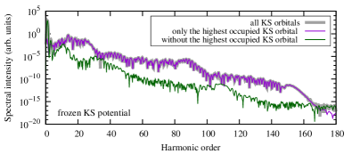
Figure 4: HHG spectra for the donor-doped system obtained from calculations with the frozen KS potential [the thick grey curve, which is the same as the upper red curve in Fig. 3(b)]. The thin purple curve and the thin green curve are obtained by Fourier transforming the partial current calculated with only the highest occupied KS orbital and without this orbital, respectively.

The role of the highest occupied impurity orbital in the donor-doped system can be highlighted within the frozen-KS-potential approach. To this end, we calculate the current from the highest occupied orbital by restricting the sum in Eq. (3) to that orbital, and compare the resulting HHG spectrum with the total one in Fig. 4. One can see that for a wide range of harmonic orders, from $\sim 10$ to $\sim 160$, the contribution from the single impurity orbital agrees with the total spectrum. Therefore we attribute the enhancement of HHG in the donor-doped system to the highest occupied impurity orbital that has an isolated energy within the BG. We note that impurity-state HHG was modeled in a recent work Almalki et al. (2018) taking only the impurity-state contribution into account when evaluating the HHG spectrum. Based on the self-consistent many-electron calculations, our present work evidences that the impurity-state HHG signal may agree with the total signal for a wide range of harmonic orders in a donor-doped band-gap material.

III.4 Semiclassical analysis of the cutoff

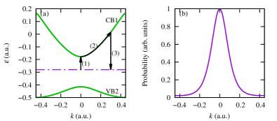
Figure 5: (a) A three-step model for HHG from the impurity-state electron, illustrated in $k$-space. The horizontal dot-dashed line indicates the donor state within the BG, i.e., the highest occupied impurity orbital for the donor-doped system. The (green) curves show the band structures of CB1 and VB2. The three steps for HHG are indicated by (black) lines with arrows. For the considered system and laser frequency, it requires at least 9 photons to excite the impurity-state electron to CB1, which is in the tunneling regime. (b) The $k$-space probability distribution of the impurity orbital depicted in (a). The first-Brillouin-zone boundary is at $k=\pi/a=0.449$.

Having demonstrated that HHG from the highest occupied impurity orbital is dominant for the donor-doped system, we now elucidate the corresponding mechanism by a semiclassical analysis. HHG from the donor-state electron can be described by a three-step model: the impurity-state electron tunnels into the conduction band, moving according to the band structure, and recombines with the impurity state when driven back by the external field. This mechanism is illustrated in $k$-space in Fig. 5(a) . Here the band-structure curves are extracted from Fig. 2 and fitted to be continuous, as done in Ref. Hansen et al. (2018). The impurity state is depicted as a completely flat band, since its $k$-space distribution spreads over the first Brillouin zone [see Fig. 5(b)]. Similarly to the semiclassical model of interband HHG in solids Vampa et al. (2015b); Vampa and Brabec (2017), we estimate the cutoff for HHG from the impurity-state electron. First, the tunneling step is considered to occur at $k_{0}=0$ corresponding to the minimum of the conduction band energy. With the tunneling time denoted by $t_{i}$, the electron trajectory after tunneling is given as Vampa et al. (2015b); Vampa and Brabec (2017)

$$x(t)-x_{i}=\int_{t_{i}}^{t}d\tau\nabla_{k}\mathcal{E}_{c}[k(\tau)],\quad k(\tau)=A(\tau)-A(t_{i}),$$ (4)

where $\mathcal{E}_{c}[k(\tau)]$ is the band structure of CB1 and $x_{i}=0$ is the initial position of the electron. When the electron returns to its initial position at time $t_{r}$, it recombines to the impurity state, emitting an energy of $\mathcal{E}_{c}[k(t_{r})]-\varepsilon_{i}$ with $\varepsilon_{i}$ the impurity-state energy. Since there is no hole motion in the valence band, the three-step model for impurity-state HHG is more atomiclike than that for solid HHG. The only difference compared with the three-step model for atomic HHG is that the electron motion after tunneling is determined by the band structure $\mathcal{E}_{c}(k)$, rather than the free-space dispersion relation $\mathcal{E}(k)=k^{2}/2$.

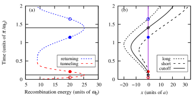
Figure 6: (a) The mapping between recombination energies (in units of $\omega_{0}=0.0114$) and semiclassical trajectories (characterized by tunneling and returning times), within one cycle of a sinusoidal vector potential with amplitude $A_{0}=0.22$. Zero on the vertical axis means a time at which the vector potential is 0. A recombination energy is associated with a pair of trajectories (referred to as long and short, in terms of the time difference between tunneling and returning). An example of long (short) trajectories is indicated by the empty (filled) circles. The horizontal lines indicate a pair of tunneling and returning times that produce the maximum recombination energy, i.e., the cutoff trajectory. (b) A real-space view of the cutoff trajectory and the example pair of long and short trajectories indicated in (a). The tunneling and returning times are marked on the vertical line $x=0$ corresponding to the impurity center. The separation between two neighboring nuclei is $a=7$ in our model.

By searching for the maximum recombination energy with different tunneling times taken into consideration, we estimate the cutoff of impurity-state HHG. Note that the trajectories in the semiclassical analysis are characterized by tunneling and returning times, and a recombination energy is associated with a pair of trajectories (referred to as long and short, in terms of the time difference between tunneling and returning of the electron). As an illustration, we show in Fig. 6(a) the mapping between recombination energies and trajectories, for the considered laser parameters. The maximum recombination energy found by the semiclassical analysis corresponds to the $25$-th harmonic, which agrees well with the observed cutoff for the donor-doped system in Fig. 3. We also present in Fig. 6(b) a real-space view of the cutoff trajectory and a pair of long and short trajectories. One can see that the impurity-state electron can move many unit-cell distances away from the impurity ion.

We mention in passing that a cutoff analysis based on the three-step model for solid HHG was also performed for the undoped system, and the corresponding cutoff estimated from the semiclassical electron-hole dynamics also agrees with that observed for the undoped system in Fig. 3. Here we focus on the first cutoff in the semiclassical analysis, since the harmonics up to the first cutoff are of more practical interest due to their relatively stronger signals. Explanation for higher cutoffs would require a model accounting for more complicated processes, which is beyond the scope of this work. So far the harmonics beyond the first cutoff are seldom measured experimentally Ndabashimiye et al. (2016). Our work indicates that experimental observation of such high-order harmonics might be less difficult for donor-doped materials.

IV Conclusion

In summary, we found that a donor-doped band-gap material can produce HHG much more efficiently than undoped and acceptor-doped materials. This significant enhancement of HHG stems from the highest occupied impurity state with an isolated energy within the BG. In contrast to HHG described by electron-hole dynamics in undoped solids, HHG from the impurity-state electron is more atomiclike, i.e., the electron moving in the conduction band will recombine with the impurity state rather than a moving hole in the valence band. The mechanism of the impurity-state HHG can be described by a three-step model where the impurity-state electron tunnels into the conduction band and then moves according to the conduction band structure until recombination. This leads to a harmonic cutoff different from that in the undoped case, which can be explained by semiclassical analysis based on the band structure. Our present work implies that donor-doped band-gap materials would be suitable for efficient generation of coherent VUV and XUV radiation. Exploring ultrafast processes in doped materials with HHG will be interesting for future work.

*

Appendix A Impurity orbitals in real space

The KS orbitals obtained from the field-free calculations can be chosen to be real-valued. In Figs. 7(a) and (b), we provide a real-space view of the energy-isolated orbitals identified from Figs. 2(b) and (c). For the considered model with $N=101$ nuclei, the number of occupied orbitals is $N_{\downarrow}=N_{\uparrow}=202$, $201$ and $203$ for the undoped, acceptor-doped and donor-doped systems, respectively. Thus the orbital with index $j=202$ in Fig. 7(a) is the lowest-unoccupied for the acceptor-doped system while the orbital with index $j=203$ in Fig. 7(b) is the highest occupied for the donor-doped system. One can see that the impurity orbitals are located around the impurity ion, spreading over a few neighboring ions.

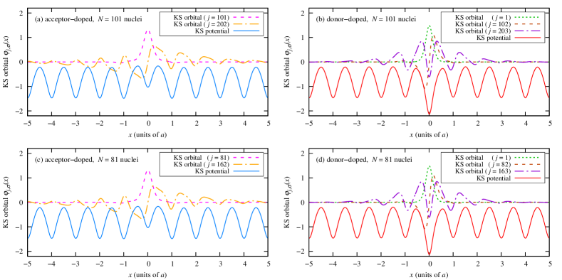
Figure 7: (a) A real-space view of the energy-isolated orbitals for the acceptor-doped system with $N=101$ nuclei. The orbitals with index $j=101$ and $j=202$ correspond to the lower and upper isolated energies in Fig. 2(b), respectively. (b) A real-space view of the energy-isolated orbitals for the donor-doped system. The orbitals with index $j=1$, $j=102$ and $j=203$ correspond to the isolated energies marked by arrows in Fig. 2(c), from bottom to top. In both acceptor- and donor-type doping cases, the corresponding KS potentials are shown for an illustrative view of the impurity and its neighboring ions. The lower panels (c) and (d) present the impurity orbitals for smaller doped systems with $N=81$ nuclei. In our model, the separation between two neighboring nuclei, i.e., the unit-cell length, is $a=7$.

We also show the impurity orbitals for smaller doped systems with $N=81$ nuclei in Figs. 7(c) and (d). Compared with Figs. 7(a) and (b), this variation of the system size does not cause any discernible change of the KS potential and the impurity orbitals. Note that for the model with $N=81$ nuclei, the number of occupied orbitals is $N_{\downarrow}=N_{\uparrow}=162$, $161$ and $163$ for the undoped, acceptor-doped and donor-doped systems, respectively. The indexes of the impurity orbitals in Figs. 7(c) and (d) are therefore different from those in Figs. 7(a) and (b). The energies of the impurity orbitals are, however, not affected, because of the negligible change of the KS potential and the impurity orbitals. In the frozen-KS-potential approach, the HHG processes are simulated by propagating the KS orbitals in the frozen KS potential, and it is shown in Fig. 4 that the highest occupied impurity-state orbital determines the total HHG spectrum for a wide range of harmonic orders in the case of donor-type doping. Thus we infer that our discussion of the impurity effects is insensitive to the system size considered in our simulations, as long as the system is sufficiently large (e.g., with more than $\sim 80$ nuclei) such that it behaves like a solid and contains the real-space motion of the impurity-state electron.

Although our discussion of doping effects is based on TDDFT simulations in a model, the underlying physics of the impurity-state HHG should be true for a real band-gap material. Since the doping-induced impurity orbitals are spatially localized around the impurity ion, we expect our results to be qualitatively valid for a target system with more than one impurity ion, as long as the impurity ions are many unit-cell distances away from each other.

References

- Krause et al. (1992) J. L. Krause, K. J. Schafer, and K. C. Kulander, “High-order harmonic generation from atoms and ions in the high intensity regime,” Phys. Rev. Lett. 68, 3535 (1992).
- L’Huillier and Balcou (1993) A. L’Huillier and P. Balcou, “High-order harmonic generation in rare gases with a 1-ps 1053-nm laser,” Phys. Rev. Lett. 70, 774 (1993).
- Krausz and Ivanov (2009) F. Krausz and M. Ivanov, “Attosecond physics,” Rev. Mod. Phys. 81, 163 (2009).
- Ghimire et al. (2011) S. Ghimire, A. D. DiChiara, E. Sistrunk, P. Agostini, L. F. DiMauro, and D. A. Reis, “Observation of high-order harmonic generation in a bulk crystal,” Nat. Phys. 7, 138 (2011).
- Schubert et al. (2014) O. Schubert, M. Hohenleutner, F. Langer, B. Urbanek, C. Lange, U. Huttner, D. Golde, T. Meier, M. Kira, S. W. Koch, et al., “Sub-cycle control of terahertz high-harmonic generation by dynamical Bloch oscillations,” Nat. Photon. 8, 119 (2014).
- Luu et al. (2015) T. T. Luu, M. Garg, S. Y. Kruchinin, A. Moulet, M. T. Hassan, and E. Goulielmakis, “Extreme ultraviolet high-harmonic spectroscopy of solids,” Nature 521, 498 (2015).
- Vampa et al. (2015a) G. Vampa, T. Hammond, N. Thiré, B. Schmidt, F. Légaré, C. McDonald, T. Brabec, and P. Corkum, “Linking high harmonics from gases and solids,” Nature 522, 462 (2015a).
- Hohenleutner et al. (2015) M. Hohenleutner, F. Langer, O. Schubert, M. Knorr, U. Huttner, S. Koch, M. Kira, and R. Huber, “Real-time observation of interfering crystal electrons in high-harmonic generation,” Nature 523, 572 (2015).
- Ndabashimiye et al. (2016) G. Ndabashimiye, S. Ghimire, M. Wu, D. A. Browne, K. J. Schafer, M. B. Gaarde, and D. A. Reis, “Solid-state harmonics beyond the atomic limit,” Nature 534, 520 (2016).
- Kruchinin et al. (2018) S. Y. Kruchinin, F. Krausz, and V. S. Yakovlev, “Colloquium: Strong-field phenomena in periodic systems,” Rev. Mod. Phys. 90, 021002 (2018).
- Corkum (1993) P. B. Corkum, “Plasma perspective on strong field multiphoton ionization,” Phys. Rev. Lett. 71, 1994 (1993).
- Vampa et al. (2014) G. Vampa, C. R. McDonald, G. Orlando, D. D. Klug, P. B. Corkum, and T. Brabec, “Theoretical Analysis of High-Harmonic Generation in Solids,” Phys. Rev. Lett. 113, 073901 (2014).
- Vampa and Brabec (2017) G. Vampa and T. Brabec, “Merge of high harmonic generation from gases and solids and its implications for attosecond science,” J. Phys. B 50, 083001 (2017).
- Higuchi et al. (2014) T. Higuchi, M. I. Stockman, and P. Hommelhoff, “Strong-Field Perspective on High-Harmonic Radiation from Bulk Solids,” Phys. Rev. Lett. 113, 213901 (2014).
- Vampa et al. (2015b) G. Vampa, C. R. McDonald, G. Orlando, P. B. Corkum, and T. Brabec, “Semiclassical analysis of high harmonic generation in bulk crystals,” Phys. Rev. B 91, 064302 (2015b).
- McDonald et al. (2015) C. R. McDonald, G. Vampa, P. B. Corkum, and T. Brabec, “Interband Bloch oscillation mechanism for high-harmonic generation in semiconductor crystals,” Phys. Rev. A 92, 033845 (2015).
- Hawkins et al. (2015) P. G. Hawkins, M. Y. Ivanov, and V. S. Yakovlev, “Effect of multiple conduction bands on high-harmonic emission from dielectrics,” Phys. Rev. A 91, 013405 (2015).
- Wu et al. (2015) M. Wu, S. Ghimire, D. A. Reis, K. J. Schafer, and M. B. Gaarde, “High-harmonic generation from Bloch electrons in solids,” Phys. Rev. A 91, 043839 (2015).
- Wu et al. (2016) M. Wu, D. A. Browne, K. J. Schafer, and M. B. Gaarde, “Multilevel perspective on high-order harmonic generation in solids,” Phys. Rev. A 94, 063403 (2016).
- Guan et al. (2016) Z. Guan, X.-X. Zhou, and X.-B. Bian, “High-order-harmonic generation from periodic potentials driven by few-cycle laser pulses,” Phys. Rev. A 93, 033852 (2016).
- Du et al. (2018a) T.-Y. Du, X.-H. Huang, and X.-B. Bian, “High-order-harmonic generation from solids: The contributions of the Bloch wave packets moving at the group and phase velocities,” Phys. Rev. A 97, 013403 (2018a).
- Du et al. (2018b) T.-Y. Du, D. Tang, X.-H. Huang, and X.-B. Bian, “Multichannel high-order harmonic generation from solids,” Phys. Rev. A 97, 043413 (2018b).
- Jin et al. (2018) J.-Z. Jin, H. Liang, X.-R. Xiao, M.-X. Wang, S.-G. Chen, X.-Y. Wu, Q. Gong, and L.-Y. Peng, “Michelson interferometry of high-order harmonic generation in solids,” J. Phys. B 51, 16LT01 (2018).
- Luu and Wörner (2016) T. T. Luu and H. J. Wörner, “High-order harmonic generation in solids: A unifying approach,” Phys. Rev. B 94, 115164 (2016).
- Földi (2017) P. Földi, “Gauge invariance and interpretation of interband and intraband processes in high-order harmonic generation from bulk solids,” Phys. Rev. B 96, 035112 (2017).
- Osika et al. (2017) E. N. Osika, A. Chacón, L. Ortmann, N. Suárez, J. A. Pérez-Hernández, B. Szafran, M. F. Ciappina, F. Sols, A. S. Landsman, and M. Lewenstein, “Wannier-Bloch Approach to Localization in High-Harmonics Generation in Solids,” Phys. Rev. X 7, 021017 (2017).
- Tancogne-Dejean et al. (2017) N. Tancogne-Dejean, O. D. Mücke, F. X. Kärtner, and A. Rubio, “Impact of the Electronic Band Structure in High-Harmonic Generation Spectra of Solids,” Phys. Rev. Lett. 118, 087403 (2017).
- Hansen et al. (2017) K. K. Hansen, T. Deffge, and D. Bauer, “High-order harmonic generation in solid slabs beyond the single-active-electron approximation,” Phys. Rev. A 96, 053418 (2017).
- Hansen et al. (2018) K. K. Hansen, D. Bauer, and L. B. Madsen, “Finite-system effects on high-order harmonic generation: From atoms to solids,” Phys. Rev. A 97, 043424 (2018).
- Bauer and Hansen (2018) D. Bauer and K. K. Hansen, “High-Harmonic Generation in Solids with and without Topological Edge States,” Phys. Rev. Lett. 120, 177401 (2018).
- Murakami et al. (2018) Y. Murakami, M. Eckstein, and P. Werner, “High-Harmonic Generation in Mott Insulators,” Phys. Rev. Lett. 121, 057405 (2018).
- Silva et al. (2018) R. Silva, I. V. Blinov, A. N. Rubtsov, O. Smirnova, and M. Ivanov, “High-harmonic spectroscopy of ultrafast many-body dynamics in strongly correlated systems,” Nat. Photon. 12, 266 (2018).
- Luu and Wörner (2018) T. T. Luu and H. J. Wörner, “Measurement of the Berry curvature of solids using high-harmonic spectroscopy,” Nat. Commun. 9, 916 (2018).
- Sivis et al. (2017) M. Sivis, M. Taucer, G. Vampa, K. Johnston, A. Staudte, A. Y. Naumov, D. M. Villeneuve, C. Ropers, and P. B. Corkum, “Tailored semiconductors for high-harmonic optoelectronics,” Science 357, 303 (2017).
- McDonald et al. (2017) C. R. McDonald, K. S. Amin, S. Aalmalki, and T. Brabec, “Enhancing High Harmonic Output in Solids through Quantum Confinement,” Phys. Rev. Lett. 119, 183902 (2017).
- Du et al. (2016) T.-Y. Du, Z. Guan, X.-X. Zhou, and X.-B. Bian, “Enhanced high-order harmonic generation from periodic potentials in inhomogeneous laser fields,” Phys. Rev. A 94, 023419 (2016).
- Huang et al. (2017) T. Huang, X. Zhu, L. Li, X. Liu, P. Lan, and P. Lu, “High-order-harmonic generation of a doped semiconductor,” Phys. Rev. A 96, 043425 (2017).
- Burgess et al. (2016) T. Burgess, D. Saxena, S. Mokkapati, Z. Li, C. R. Hall, J. A. Davis, Y. Wang, L. M. Smith, L. Fu, P. Caroff, et al., “Doping-enhanced radiative efficiency enables lasing in unpassivated GaAs nanowires,” Nat. Commun. 7, 11927 (2016).
- Klyukin et al. (2018) K. Klyukin, L. L. Tao, E. Y. Tsymbal, and V. Alexandrov, “Defect-Assisted Tunneling Electroresistance in Ferroelectric Tunnel Junctions,” Phys. Rev. Lett. 121, 056601 (2018).
- Note (1) The periodic arrangement of dopants at a very high impurity concentration considered in the single-active-electron model calculations of Ref. Huang et al. (2017) is atypical and leads to a substantial change of the system.
- Runge and Gross (1984) E. Runge and E. K. U. Gross, “Density-Functional Theory for Time-Dependent Systems,” Phys. Rev. Lett. 52, 997 (1984).
- Ullrich (2011) C. A. Ullrich, Time-Dependent Density-Functional Theory: Concepts and Applications (Oxford University Press, Oxford, 2011).
- Pantelides (1978) S. T. Pantelides, “The electronic structure of impurities and other point defects in semiconductors,” Rev. Mod. Phys. 50, 797 (1978).
- Bauer (2017) D. Bauer, ed., Computational Strong-field Quantum Dynamics: Intense Light-matter Interactions (De Gruyter, Berlin, 2017).
- Slater (1949) J. C. Slater, “Electrons in Perturbed Periodic Lattices,” Phys. Rev. 76, 1592 (1949).
- Luttinger and Kohn (1955) J. M. Luttinger and W. Kohn, “Motion of Electrons and Holes in Perturbed Periodic Fields,” Phys. Rev. 97, 869 (1955).
- Kohn (1957) W. Kohn, “Shallow Impurity States in Silicon and Germanium,” Solid State Phys., 5, 257 (1957).
- Bassani et al. (1974) F. Bassani, G. Iadonisi, and B. Preziosi, “Electronic impurity levels in semiconductors,” Rep. Prog. Phys. 37, 1099 (1974).
- Keldysh (1964) L. V. Keldysh, “Ionization in the field of a strong electromagnetic wave,” Zh. Eksp. Teor. Fiz. 47, 1945 (1964), [Sov. Phys. JETP 20, 1307 (1965)].
- Almalki et al. (2018) S. Almalki, A. M. Parks, G. Bart, P. B. Corkum, T. Brabec, and C. R. McDonald, “High harmonic generation tomography of impurities in solids: Conceptual analysis,” Phys. Rev. B 98, 144307 (2018).
- Note (2) For the considered vector-potential amplitude , we simply restrict to a single conduction band, CB1, since the semiclassical electron will not reach the first-Brillouin-zone boundary [Eq. (4\@@italiccorr)].