Engineering large end-to-end correlations in finite fermionic chains

Abstract

We explore deformations of finite chains of independent fermions which give rise to large correlations between their extremes. After a detailed study of the Su-Schrieffer-Heeger (SSH) model, the trade-off curve between end-to-end correlations and the energy gap of the chains is obtained using machine-learning techniques, paying special attention to the scaling behavior with the chain length. We find that edge-dimerized chains, where the second and penultimate hoppings are reinforced, are very often close to the optimal configurations. Our results allow us to conjecture that, given a fixed gap, the maximal attainable correlation falls exponentially with the system size. Study of the entanglement entropy and contour of the optimal configurations suggest that the bulk entanglement pattern is minimally modified from the clean case.

I Introduction

Two fundamental elements in quantum many-body physics are strong correlations and entanglement Amico.08 , which constitute a basic resource in quantum communications and quantum computation Nielsen.00 and a key component of most quantum technologies. Moreover, the ground states (GS) of quantum systems are known to present very interesting entanglement properties Eisert.10 , such as the area-law: for a gapped system, the entanglement entropy of a certain block is typically proportional to the block boundary Sredniki . Gapless systems, on the other hand, usually present logarithmic corrections which can be assessed making use of conformal invariance Vidal.03 .

Some (gapless) deformed systems can violate maximally the area law and present volumetric entanglement, for example the so-called rainbow state Vitagliano.10 ; Ramirez.14 ; Ramirez.15 , a valence bond solid (VBS) where the fermionic bonds are concentrically placed around the center. It can be built as the ground state of an open chain of free fermions, whose hoppings decay exponentially from the center. Nonetheless, the energy gap for the rainbow state decays exponentially with the system size, thus making it difficult to implement in actual quantum devices.

The aim of this article is to determine deformations of a quantum independent fermionic chain which attain a maximal correlation between its extremes, while keeping an appreciable energy gap. Note that, according to Hastings’ theorem, one-dimensional (1D) gapped systems must fulfill the area law Hastings , proving that it is impossible to obtain a rainbow state as the GS of a 1D gapped Hamiltonian. Nonetheless, large end-to-end correlations on a gapped system are not explicitly forbidden.

Our study begins with the well-known Su-Schrieffer-Heeger (SSH) model of a dimerized fermionic chain Su.79 ; Heeger.88 ; Sirker.14 , whose links alternate between a weak and a strong value, which constitutes a paradigm for topological insulators Asboth . When the first and last links are weak, an edge state can appear in the form of a valence bond between the first and last sites, thus inducing a large correlation between them, see Fig. 1 for an illustration. Unfortunately, the energy gap required to excite away this edge state decays too fast with the system size. Yet, it will provide the essential clues to explain the optimal deformations.

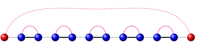
Figure 1: An open dimerized fermionic chain with alternate lighter (thinner black lines) and stronger links (thicker black lines). The stronger links will tend to form a valence bond (red line). A large distance correlation between the first and last sites may appear (indicated as a dashed red line).

Next, we developed a machine-learning algorithm to obtain the deformations which maximize the end-to-end correlation (in absolute value) for a fixed chain length and energy gap. We show that, in many cases, these configurations are edge-dimerized chains, where the second and last links are reinforced. We show that the maximal correlation obtained with our algorithm decays exponentially with the system size and with the energy gap. We would like to emphasize that this article only provides a proof-of-principle strategy to establish large correlations among distant sites of a quantum system while retaining a large enough gap. Thus, our conclusions regarding the scaling behavior of the maximal correlation remain tentative and need further work.

This article is organized as follows. Sec.II presents the model employed, independent lattice fermions. Dimerized open chains are discussed in Sec. III. The machine-learning procedure is described in Sec. IV, along with the results obtained for the optimal correlation. This leads to the study of edge-dimerized chains in Sec. V. Our conclusions are summarized in the last Section.

II Model

Let us consider a chain of $L$ sites where $N_{e}$ independent spinless Dirac fermions move. An inhomogeneous tight-binding Hamiltonian can be written in the following way:

$$H=-\sum_{i}t_{i}\ c^{\dagger}_{i}c_{i+1}+h.c.$$ (1)

where $c^{\dagger}_{i}$ is the creation operator at site $i$ and the $t_{i}$ are the local hopping amplitudes. We will consider $N_{e}=L/2$, i.e., half-filling. If the hoppings are homogeneous, $t_{i}=1$, the chain is called clean and can be described in the continuum limit by a conformal field theory (CFT) DiFrancesco. Please notice that we do not consider on-site disorder, i.e. inhomogeneities in the chemical potential.

The ground state (GS) of (1) can always be written as a Slater determinant:

$$\left|\Psi\right>=\prod_{k=1}^{N_{e}}b^{\dagger}_{k}\left|0\right>,$$ (2)

with $\left|0\right>$ the Fock vacuum and $b^{\dagger}_{k}$ the creation operators for the orbitals, given by a canonical transformation

$$b^{\dagger}_{k}=\sum_{i}U_{ki}\ c^{\dagger}_{i},$$ (3)

where $U$ is the matrix that diagonalizes the hopping matrix, $T_{ij}=t_{i}\ (\delta_{i,i+1}+\delta_{i,i-1})$, with eigenvalues $\varepsilon_{k}$. The energy gap of the system is given by the minimal excitation energy:

$$\Delta E=\varepsilon_{(L/2)+1}-\varepsilon_{L/2}.$$ (4)

The correlation matrix, defined as

$$C_{i,j}=\left<\Psi\right|c^{\dagger}_{i}c_{j}\left|\Psi\right>.$$ (5)

allows us to compute the expectation value of any observable on any state given by Eq. (2), via Wick’s theorem. It can be evaluated using the matrix $U$:

$$C_{i,j}=\sum_{k=1}^{N_{e}}\bar{U}_{ki}U_{kj}.$$ (6)

Notice that the local density, $\left<n_{i}\right>=\left<c^{\dagger}_{i}c_{i}\right>$, is given by the diagonal elements of $C_{i,j}$. Making use of chiral symmetry it can be proved that, at half-filling, the density must be homogeneous, i.e. $\left<n_{i}\right>=1/2$ for all $i\in\left\{1,L\right\}$ Asboth .

II.1 Entanglement of free fermionic chains

Entanglement properties of a generic block of the chain, $B=\left\{i_{1},\cdots,i_{\ell}\right\}$ (note that the sites $i_{1},\cdots,i_{\ell}$ are possibly disjointed), are always referred to the reduced density matrix of $\left|\Psi\right>$, defined as

$$\rho^{B}\equiv\mathrm{Tr}_{B}\left|\Psi\right>\left<\Psi\right|,$$ (7)

being $\mathrm{Tr}_{B}$ the corresponding partial trace. In the case of a Slater determinant, this $\rho^{B}$ can be expressed as a tensor product of $2\times 2$ density matrices of the form Peschel.03

$$\rho^{B}=\bigotimes_{k=1}^{\ell}\begin{pmatrix}\nu^{B}_{k}&0\\ \\ 0&1-\nu^{B}_{k}\end{pmatrix}.$$ (8)

where the $\nu^{B}_{k}\in[0,1]$ are the eigenvalues of the correlation $\ell\times\ell$ sub-matrix corresponding to the block $C^{B}$ (i.e., those elements of $C_{i,j}$ with $i,j\in B$).

As a measure of the entanglement between the block and the rest of the system we choose the von Neumann entropy of $\rho^{B}$,

$$S^{B}=-\mathrm{Tr}\rho^{B}\log\rho^{B},$$ (9)

which can be computed using the following expression Peschel.03

$$S^{B}=-\sum_{k=1}^{\ell}\Big{(}\nu_{k}^{B}\log\nu_{k}^{B}+(1-\nu_{k}^{B})\log(1-\nu_{k}^{B})\Big{)}.$$ (10)

Our interest in the aforementioned entanglement measures stems from the fact that they are usually able to characterize the different phases of matter through e.g. corrections (or violations) to the area law for the entanglement entropy Vidal.03 ; Ramirez.14 .

It is also relevant to ask about the spatial origin of entanglement within a block. An entanglement contour $s^{B}(i)$ Vidal.14 is defined as a distribution of the block entanglement among the sites with some obvious properties, such as positivity and completeness:

$$\sum_{i=1}^{\ell}s^{B}(i)=S^{B},\qquad s^{B}(i)\geq 0.$$ (11)

A concrete proposal for an entanglement contour for free fermions was made by Chen and Vidal Vidal.14 , which has been shown to match the CFT prediction Tonni.18 . The expression is given by

$$s^{B}(i)=-\sum_{k=1}^{\ell}|V^{B}_{ki}|^{2}\big{(}\nu_{k}^{B}\log\nu_{k}^{B}+(1-\nu_{k}^{B})\log(1-\nu_{k}^{B})\big{)}.$$ (12)

where $V^{B}_{ki}$ is the $i$-th component of the $k$-th eigenvector of the correlation sub-matrix $C^{B}$. Both properties in Eq. (11) are straightforward to prove. Let us remark that the entanglement contour has already been employed to provide insight into the study of quantum phases of matter Tonni.18 ; Alba.18 .

II.2 Dasgupta-Ma Renormalization

When the values of the hoppings are very different among themselves, a useful approximation is provided by the Dasgupta-Ma renormalization scheme Dasgupta.80 ; Ramirez.14b , a second-order perturbation theory approach which was initially devised for random spin chains and, thus, it is known as strong disorder renormalization group (SDRG). We should stress that the main requirement for the applicability of the SDRG is not disorder, but strong inhomogeneity, as shown in the applicability to e.g. the rainbow chain Ramirez.14 ; Ramirez.15 ; Laguna.16 . When the inhomogeneity of the hoppings is not so strong, the accuracy of the SDRG algorithm will decrease. Yet, it has been shown in a variety of cases that as the inhomogeneity is decreased, the exact GS undergoes a smooth crossover between the SDRG prediction and the homogeneous (or clean) GS Ramirez.14b ; Ramirez.15 ; Laguna.17 ; Tonni.18 .

In order to obtain the GS of Hamiltonian (1) on a generic system with strongly inhomogeneous hoppings, the SDRG proceeds in an iterative way by always selecting the strongest link and putting a valence bond between the two sites with this strongest link. Next, the neighboring sites to this bond are linked by an effective hopping which is found using second-order perturbation theory Dasgupta.80 ; Ramirez.15 :

$$t^{\mathrm{eff}}=-\frac{t_{L}\ t_{R}}{t_{\mathrm{\mathrm{max}}}},$$ (13)

where $t_{L}$ and $t_{R}$ are the left and right hoppings, and $t_{\mathrm{max}}$ is the maximal hopping (in absolute value). Notice that the effective hopping can have different signs. At half-filling, the algorithm proceeds until all sites are part of one of such valence bonds. Thus, the GS can be described as a valence bond solid (VBS). The energy gap, $\Delta E$, can be estimated making use of the SDRG. It corresponds to the (effective) hopping of the last bond Ramirez.14b .

It has been recently proved Alba.18 that, in the case of free fermions, when a bond is formed between sites $i$ and $j$ of a 1D chain, the effective hopping within SDRG is always given by

$$t_{i,j}^{\mathrm{eff}}=\frac{t_{i}\;t_{i+2}\;t_{i+4}\cdots t_{j-1}}{t_{i+1}\cdots t_{j-2}},$$ (14)

i.e. the product of the odd hoppings divided by the product of the even ones. Thus, when a valence bond is established between the two extreme sites of a chain, it will usually have the lowest energy and Eq. (14) provides an estimate for the energy gap of the system.

III Dimerized chains

Let us consider a dimerized version of the Hamiltonian given by Eq. (1), using

$$t_{i}=1+(-1)^{i}\ \delta,$$ (15)

with $\delta\in[0,1)$. Thus, the first and last hoppings are always weaker, $t_{1}=t_{L-1}=1-\delta$. This is, indeed, the Su-Schrieffer-Heeger (SSH) Hamiltonian Su.79 ; Heeger.88 ; Sirker.14 specialized for the topologically non-trivial phase Asboth , where an edge state appears between the first and last sites. See Fig. 1 for an illustration. For large enough $\delta$, the fermions minimize their energy by localizing on valence bonds on top of the stronger links, $t_{2k}=1+\delta$, for all $k<L/2$. After all these bonds are formed, the remaining fermion, being unable to be localized on those hoppings, will be delocalized around the sites 1 and $L$.

This dimerization appears naturally in 1D systems due to the Peierls distortion Peierls.qts ; Peierls.surprises : the coupling between electrons and phonons on 1D lattices can give rise to a new spatial periodicity, twice the original one, opening a gap at the Fermi energy. For example, a quasi-1D polymer like trans-polyacetylene is electrically insulating whereas the configuration with all links equivalent is metallic. The Peierls transition is a widespread phenomenon in quasi 1D systems, making dimerized materials more energetically favorable than other structural phases in many occasions Gruner.88 ; Snijders.10 .

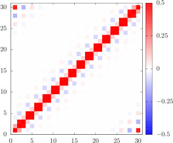
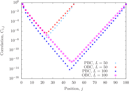
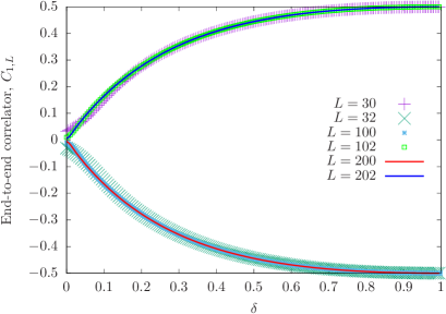
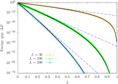
Figure 2: Top-left: Correlation matrix, $C_{i,j}$ for the GS of the $L=30$ open dimerized chain with hoppings given by Eq. (15) and dimerization parameter $\delta=0.5$. Notice the dimerization pattern along the secondary diagonals, and the large non-local correlations between sites $1$ and site $L$. Top-right: Absolute value of the correlation function $C_{1,j}$ in logarithmic scale, for both open (OBC) and periodic (PBC) boundary conditions, for $L=50$ and $L=100$ and $\delta=0.5$. Notice the similarity between them. Bottom-left: end-to-end correlation obtained in an open dimerized chain of the form Eq. (15) as a function of $\delta$ for several values of $L$, showing the collapse. Bottom-right: energy gap of the system; the dashed straight lines represent exponential decays, $\exp(-L\ \delta/2)$. The continuous black lines correspond to the simple theoretical estimate given by Eq. (17).

The top-left panel of Fig. 2 presents the correlation matrix $C_{ij}$ of a chain with $L=30$ sites when $\delta=0.5$, as computed using Eq. (6). Notice that all the diagonal elements equal $1/2$, because in this case the fermionic density at the sites can be proved to be homogeneous (summing up all occupied states, we have a constant local density of states on all the sites of the system, even with this distinct correlation pattern). The off-diagonal elements, then, show the correlations in our system. All matrix elements of the form $C_{2k,2k+1}$ take a much higher value than those of the form $C_{2k-1,2k}$, showing a strong dimerization. The value $C_{1,L}$ is also high, signaling the expected presence of an edge-state Asboth . We will call that term the end-to-end correlation.

The top-right panel of Fig. 2 shows, in logarithmic scale, the absolute value of the correlation between site 1 and all others, comparing two sizes ($L=50$ and $100$) and two types of boundary conditions (open (OBC) and periodic (PBC)). Note that the results for the correlation function $C_{1,j}$ at the end of the chains (i.e., for $j=50$ and $100$, respectively) are about $1/2$ for both open and periodic conditions. The periodic case is well known: $C_{1,j}$ falls exponentially until $j\sim L/2$ (the center of the chain), where it becomes quite small; then it raises exponentially again. Interestingly, the same large decay and increase takes also place for open boundaries.

In the bottom-left panel of Fig. 2 we have plotted this end-to-end correlation, $C_{1,L}$ as a function of the dimerization parameter $\delta$ for open systems of different sizes. The correlation sign depends on whether the value of $L\allowbreak\mkern 5.0mu({\operator@font mod}\,\,4)$ equals 0 or 2, because of the parity of the number of fermions in the chain bulk. The collapse of all curves with the same parity for different system sizes is remarkable.

It is relevant to ask about the stability of these large end-to-end correlations, i.e., what is the effective hopping associated to them, directly related with the energy gap $\Delta E$, given by Eq. (4). The bottom-right panel of Fig. 2 shows this energy gap as a function of $\delta$ for different system sizes. Notice the exponential decay for small $\delta$, becoming even faster for larger dimerizations. The dashed lines correspond to the exponential behavior,

$$\Delta E\sim\exp(-L\,\delta/2).$$ (16)

Yet, the behavior of the energy gap along all the range for $\delta$ can be successfully estimated making use of the SDRG approximation. Indeed, Eq. (14) can be applied to our case, using the expression for the hoppings given in Eq. (15), and obtaining

$$t_{1,L}^{\mathrm{eff}}=\frac{(1-\delta)^{L/2}}{(1+\delta)^{L/2-1}}.$$ (17)

This effective SDRG hopping between the two extremes is a good approximation for the energy gap as shown by the black continuous curves on the bottom-right panel of Fig. 2, which fit the numerical results for $\Delta E$ with remarkable accuracy over several orders of magnitude.

Unfortunately, this result also leads to a predictable conclusion: since the energy gap $\Delta E$ is so small, the edge states of the SSH model are extremely fragile.

III.1 Entanglement properties of the dimerized chain

The introduction of dimerized hoppings on a clean free-fermionic infinite chain decrease notably the correlations on the GS, see the bottom-left panel of Fig. 2. Moreover, the appearance of an energy gap forces the state to fulfill the area-law Hastings , thus making the maximal entropy bounded. It is interesting to consider the entanglement properties of finite SSH chains in order to determine with more accuracy the different contributions of the bulk and the edge. Remarkably, a low degree of dimerization has been shown to increase the entanglement between the left and right halves of the system with respect to the clean case Sirker.14 ; Sedlmayr.18 , and this increase in entanglement entropy has been suggested as a mechanism behind the Peierls transition Sirker.08 ; Sirker.14 . In this section we intend to extend previous findings about the entanglement behavior of the SSH chain Sirker.14 ; Sedlmayr.18 with the use of the entanglement contour Vidal.14 . This, in turn, will help us in our main aim of establishing stable quantum chains with large end-to-end correlations.

The top panel of Fig. 3 shows the entanglement entropy of blocks comprising the $\ell$ leftmost sites, $S(\ell)$, obtained with Eq. (10) for different values of $\delta$ in an open dimerized chain with $L=128$. In the figure, it can be seen how the entanglement entropy $S(\ell)$ increases as $\delta$ increases. The amplitude of the oscillations also increases, as for $\delta\to 1^{-}$ the system becomes a valence bond solid. For zero dimerization, $\delta=0$, $S(\ell)$ almost reproduces the well-known form obtained from CFT Vidal.03 ; Calabrese.04 ,

$$S=\frac{1}{6}\log\Bigg{(}\frac{L}{\pi}\sin\left(\frac{\pi\ell}{L}\right)\Bigg{)}+Y(\ell)$$ (18)

where the first term is provided by the CFT and $Y(\ell)$ is a non-universal mild oscillatory term Calabrese.09 ; Xavier.11 .

On the other side, as commented, in the $\delta\to 1^{-}$ limit the GS becomes a valence bond solid (VBS). In that regime, entanglement entropies of given blocks are easy to estimate: one must simply count the number of broken bonds when the block is separated from the environment, and multiply by $\log(2)$. In this strong dimerization regime, the block entanglement entropy $S(\ell)$ becomes exactly oscillating, alternating values of $\log(2)$ (single bond cut) and $2\log(2)$ (two bonds cut), as depicted in the physical picture shown in Fig. 1.

The central panel of Fig. 3 shows $S(L/2)$ (i.e. the entanglement entropies for the half chain) as a function of $\delta$ for several system sizes, always choosing multiples of 4 in order to have two bond cuts in the strongly dimerized limit. We observe a fast linear increase of the entropy for low values of $\delta$, reaching a maximum that increases with the system size. Beyond that maximum, the entropy for all different sizes collapse to a single curve which approches asymptotically the limit value $S(L/2)\to 2\log(2)$ for $\delta\gtrsim 0.15$. Notice also that we have included the computation for $\delta<0$, obtaining lower values of the entanglement entropy that also collapse.

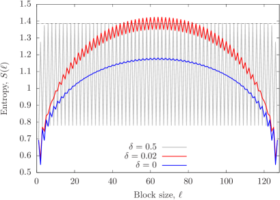
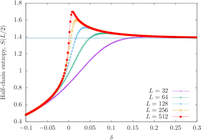
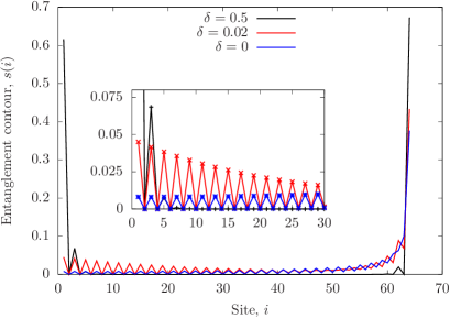
Figure 3: Top: Entanglement entropy of blocks $\left\{1,\cdots,\ell\right\}$ as a function of the block size $\ell$ for different values of $\delta$, using $L=128$, on the GS of an open dimerized chain given by Eq. (15). Center: Half-system entanglement entropy $S(L/2)$ as a function of the dimerization parameter, for different values of $L$. Notice the initial linear surge, followed by a monotonous (exponential) decay towards $2\log(2)$, indicated by horizontal lines in both panels. Bottom: entanglement contour for the left half of the $L=128$ system and the same values of $\delta$ used for the top panel. Inset: zoom on the left part of the block.

It is enlightening to consider the entanglement contour, defined in Eq. (12), for the left half of the chain with $L=128$ sites, using $\delta=0$, $0.02$ and $0.5$, as shown in the bottom panel of Fig. 3. Notice that the left extreme corresponds with the physical left boundary of the chain, while the right extreme of the plot corresponds with the center of the chain. We can see that for large $\delta$ (black curve) the entanglement contour is large at both extremes, and small everywhere else. The reason is that only sites $1$ and $L/2$ contribute to the block entanglement, because they take part in broken valence bonds. For $\delta=0$ we recover the conformal case Tonni.18 , where it is known that the entanglement contour falls as a power law, $s(i)\sim(L/2-i)^{-1}$. For the selected intermediate value, $\delta=0.02$, we see that the contour on the right extreme of the block is very similar to the clean case ($\delta=0$). Nonetheless, we also observe that the contour on the left half has risen considerably. Thus, we can argue that the entanglement excess is produced in the bulk, but due to a boundary effect Sedlmayr.18 .

Our preliminary conclusions from this study are that (a) dimerization at the edge of the chain can give rise to strong end-to-end correlations; (b) the energy gap is enormously reduced due to the bulk dimerization (see Eq. (17)) and (c) the initial surge in entropy when we dimerize a clean chain (see central panel of Fig. 3) is a bulk phenomenon. These conclusions will help us in the following sections.

IV Correlation engineering in chains

Can we obtain large end-to-end correlations in a fermionic chain with a large enough energy gap?

Let us consider an open chain with $L$ sites and $N_{e}=L/2$ fermions, described by Eq. (1). The absolute value of the end-to-end correlation, $|C_{1,L}|$ can be regarded as a function of the hopping amplitudes, $\left\{t_{i}\right\}_{i=1}^{L-1}$. We can now obtain the maximum of this function with the energy gap constrained to take a fixed value $\Delta E$, Eq. (4), using an optimization algorithm. In order to avoid a trivial increase of the energy gap through a rescaling of the hopping terms, we will normalize it with the average value of the hoppings, $\bar{t}$ (all hoppings will be restricted to be positive).

The aforementioned optimization is a non-trivial task, due to the complex landscape exhibited by the target function Weise ; Schrijver . It has been recently shown that machine-learning techniques can be suitable for the solution of quantum many-body problems Carleo.17 ; Fujita.18 . In this work we employ numerical techniques inspired in machine-learning in order to obtain the desired optimal hoppings in an efficient way.

IV.1 Machine-learning technique

The optimizer algorithm receives two parameters: the system length, $L$, and the expected value of the energy gap $\Delta E_{0}$. The target function is defined as

$${\cal F}\left(\left\{t_{i}\right\}_{i=1}^{L-1}\right)\equiv|C_{1,L}|-K\left|{\Delta E-\Delta E_{0}\over\bar{t}}\right|.$$ (19)

where $K$ is a constraint coefficient, which is varied along the algorithm, ultimately reaching a very large value in order to ensure that the energy constraint is fulfilled. Notice that the energy gap is always measured in units of the average hopping.

The algorithm starts out with $N_{c}$ random configurations (typically, $N_{c}=8$) for the hoppings with fixed average, $\bar{t}=1$. A conjugated gradients NRC search is performed on each of these initial configurations in three stages, increasing progressively the value of $K$ (typically, $K_{1}=1$, $K_{2}=100$ and $K_{3}=10^{4}$). After this procedure, the best $N_{c}/2$ configurations are stored with a small random perturbation. We add $N_{c}/2$ new random configurations and the cycle repeats again. After a few cycles (always less than $10$), the best configuration is selected.

IV.2 Results: optimal chains

In the top-left panel of Fig. 4 we present the optimal hopping amplitudes for $L=40$ with a few values of the fixed energy gap $\Delta E=0.01$, $0.05$, $0.1$ and $0.2$ (always in units of the average hopping, $\bar{t}$), which give rise to maximal (negative) end-to-end correlations $-0.384$, $-0.221$, $-0.107$ and $-0.021$ respectively. The systematic study of the maximal correlation achievable for a given gap is performed in the next section. At this moment, let us explore the resulting hopping profiles.

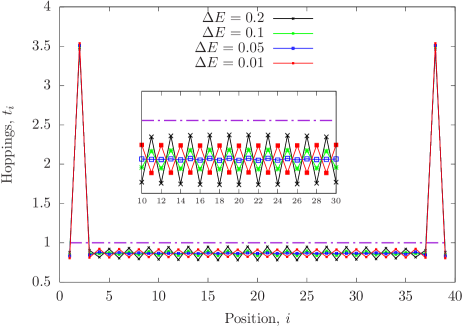
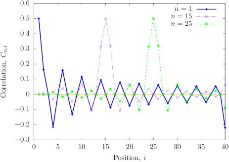
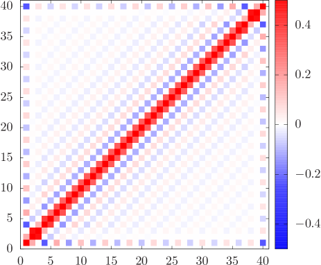
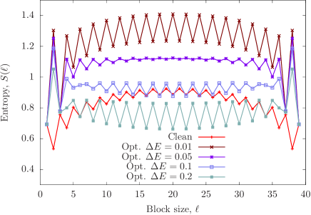
Figure 4: Optimizing the end-to-end correlation in an open fermionic chain with $L=40$ sites for a fixed gap and average hopping fixed to 1. Top-left: optimal hoppings for fixed gaps $\Delta E=0.2$, 0.1, 0.05 and 0.01. Notice that, in all cases, the dimerization is strongly modulated, with the second and penultimate hoppings always significantly stronger than the rest. Inset: zoom of the previous data in the central zone. Notice that the dimerization is opposite in very low and large gaps. Top-right: correlation functions $C_{n,i}$ for selected sites, $n=1$, $15$ and $25$ for the case $\Delta E=0.05$. The $n=1$ shows a strong peak at the end, with an end-to-end correlation $C_{1,L}\approx-0.221$. Bottom-left: full correlation matrix for the $\Delta E=0.05$ case. Bottom-right: block entropies for the cases shown in the top-left panel.

The optimal hopping profiles shown in the top-left panel of Fig. 4 show a strongly modulated dimerization. Indeed, the second and penultimate links become significatively stronger, with $t_{2}=t_{L-2}\approx 3.5$. This edge-dimerization is present in the optimal hopping patterns for all target values of $\Delta E$. On the other hand, the dimerization amplitude is much smaller in the bulk. The inset of the top-left panel of Fig. 4 still shows another interesting surprise: the bulk dimerization takes a different phase for large and smaller values of the energy gap $\Delta E$. Indeed, for small gap ($\Delta E=0.01$, red line) the dimerization phase is the same as in the previous section (pattern $(1-\delta),(1+\delta),\cdots,(1-\delta)$). But the pattern is reversed for larger values of the gap. The reason can be understood via Eq. (14). The energy gap grows by shifting the large hopping values to the numerator and the small ones to the denominator, at the expense of reducing the end-to-end correlation.

The top-right panel of Fig. 4 shows the correlation function, $C_{n,i}$ for several values of $n$ ($n=1$, $15$ and $25$) in the case of $\Delta E=0.05$, when the dimerization amplitude is minimal among all the cases shown in the left panel. We observe that the end-to-end correlation is negative, $C_{1,L}=-0.221$, and that the amplitudes of the correlation function, $C_{1,i}$, decay very slowly with the distance from the origin. For the other cases, $C_{15,i}$ and $C_{25,i}$, we see a much faster decay. The bottom-left panel of Fig. 4 presents the correlation data for the previous case ($L=40$, $\Delta E=0.05$) in matrix form, where we can observe the large end-to-end correlation in the upper-left and lower-right corners.

Therefore, we can conjecture the following theoretical propostion: if some sites form strong bonds with their neighbors and as a consequence some sites are left isolated, these isolated sites are forced to establish large correlations between them, even if they are at a long distance. Of course, these long-distance bonds will be weaker. As discussed above, the energy gap can be estimated using the effective hopping amplitude obtained through the generalized SDRG expression, Eq. (14). This effective hopping amplitude takes a large value when only the second and penultimate hoppings are large, while the rest are all equal. This result leads to the conjecture that edge-dimerized chains will be always close to providing robust optimal correlations.

The bottom-right panel of Fig. 4 shows the block entanglement entropies of the optimal configurations obtained, $S(\ell)$, compared to the homogeneous case given by CFT, Eq. (18). We can observe that for very low $\Delta E=0.01$ the entanglement shifts vertically and acquires stronger parity oscillations. The vertical shift ($\sim\log(2)$) is due to the long bond between the two extremes of the chain, and the parity effect due to the dimerization. When $\Delta E=0.05$ the hoppings on the bulk presented the minimal dimerization, and we can see a corresponding flattening of the entropy curve. In all cases we can see that the entropy of the block of 2 sites, $S(2)\sim 2\log(2)$. This means that both site 1 and 2 establish a valence bond with some other sites. In fact, site 1 attempts to establish the bond with site $L$, while site 2 is strongly connected to site 3. This fact is checked by observing that the entropy of the block of 3 sites, $S(3)\sim\log(2)$, because this block contains now a full valence bond plus the broken bond corresponding to site 1. For larger values of $\Delta E$, we see the entropy decaying while keeping the edge behavior.

IV.3 Scaling limit: larger optimal chains

The previously discussed results have an intrinsic interest, since they allow us to engineer robust devices of nanoscopic scale ($\sim 50$ atoms) with large correlations. Yet, it is relevant to ask whether this effect can be extended to larger system sizes.

Fig. 5 shows the maximal attainable correlation as a function of the system size, $L$, for different values of the energy gap, $\Delta E$. In all cases, the maximal correlation decays exponentially, with a certain effective length which depends on the energy gap,

$$|C_{1,L}|\sim\exp\left(-L/L_{\mathrm{eff}}(\Delta E)\right).$$ (20)

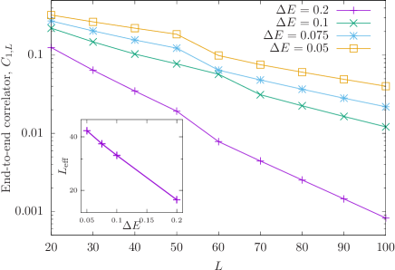
Figure 5: Scaling behavior of the optimal correlation $C_{1,L}$, obtained as a function of the system size $L$, for given values of the (fixed) energy gap $\Delta E$. In all cases, the maximal correlation decays exponentially with the system size, Eq. (20). Inset: behavior of the effective length with the energy gap, $L_{\mathrm{eff}}(\Delta E)$.

It is remarkable that, despite the general exponential trend of all curves in Fig. 5, they all present some glitch at a finite value of $L$. This is typically due to a change in the dimerization pattern of the optimal configuration. The dependence of the effective length on the energy gap, $L_{\mathrm{eff}}(\Delta E)$, is shown in the inset of Fig. 5. We can see that it also decays exponentially:

$$L_{\mathrm{eff}}\sim\exp\left(-\Delta E/\Delta E_{*}\right),$$ (21)

where $\Delta E_{*}\sim 0.17$.

Therefore, the results presented in this section lead us to conjecture that, in order to obtain the maximal end-to-end correlation in a fermionic chain keeping a large energy gap, the best strategy is usually to induce a strong dimerization at the edge with a homogeneous bulk. Yet, the maximal correlation for a fixed energy gap will always decrease exponentially.

V Modulated and Edge Dimerization

V.1 Modulated dimerized chains

The results regarding the optimized correlations presented in Section IV hint at a conjecture: a modulated dimerization may achieve strong end-to-end correlations with a broader energy gap. We will explore that conjecture along this section. The modulation is achieved by allowing the dimerization parameter to vary along the open boundary chain. Let us introduce a continuous modulation function $\delta(x):[-1,1]\mapsto{\mathbb{R}}^{+}$ and its discretized version:

$$\delta_{i}=\delta\left({i-L/2\over L/2}\right).$$ (22)

Now, let the Hamiltonian take the following form:

$$H=-\sum_{i}^{L-1}\big{(}1+(-1)^{i}\ \delta_{i}\big{)}\;c^{\dagger}_{i}c_{i+1},$$ (23)

Notice that, by construction, the average value of the hopping terms is always one. Thus, the energy scale is fixed, and we can use the energy gap in the spectrum to measure the stability of the GS. Also notice that, in all cases, the first and last hoppings will be weaker.

We have explored several possibilities for the dimerization function $\delta(x)$, always increasing the dimerization towards the extremes, and symmetrical with respect to the center of the chain.

(a) No modulation, as in Sec. III, $\delta(x)=\delta_{0}$.

(b) Linear modulation, $\delta(x)=\delta_{0}\ |x|$.

(c) Quadratic modulation, $\delta(x)=\delta_{0}\ x^{2}$.

(d) Exponential modulation, given by the expression

$$\delta(x)=\delta_{0}\exp\left(\lambda(|x|-1)\right).$$ (24)

In Fig. 6 we present the results for the relationship between the energy gap, $\Delta E$, and the end-to-end correlation, $C_{1,L}$, for these different dimerization schemes on open fermionic chains using the Hamiltonian (23)

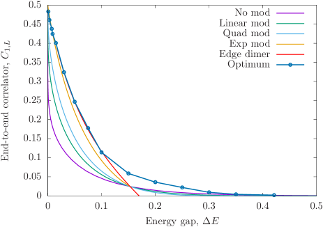
Figure 6: End-to-end correlation in open chains, $C_{1,L}$, as a function of the energy gap, $\Delta E$, for different chain types whose hoppings are subject to a modulated dimerization, Eq. (23). Different values of $\delta_{0}$ (or $t_{0}$) lead to different points of the curve. The different modulation types are: no-modulation; linear modulation; quadratic modulation; exponential modulation (Eq. (24) with $\lambda=8$). All these cases are compared to the optimum, obtained using the machine learning procedure of Sec. IV (thicker line). We also show the edge-dimerization results discussed in Sec. V.2 (red line) that present very similar results to the optimal hoppings for energy gaps $\Delta E\lesssim 0.125$.

We can see that, in all cases under study, the end-to-end correlation decreases with the gap. We have added a last curve, given by the optimal correlation for each given value of the energy gap, as obtained through the machine-learning algorithm of Sec. IV. We should remark that the optimal curve remains above the correlation curve for all types of modulation, as expected. Yet, we can see that the exponential modulation (yellow line) is, among the proposed functions $\delta(x)$, the one that comes closest to the optimal one. Again, we see that strong dimerization near the edges and weak dimerization in the bulk leads to larger values of the end-to-end correlation, for a fixed energy gap. Thus, it is natural to take the next step, and dimerize only the edges of the chain.

V.2 Edge-dimerized chains

Let us consider an open fermionic chain of $L$ (even) sites, where all hoppings $t_{i}=1$ except two, $t_{p}=t_{L-p}=t_{0}$. We will only use small values of $p$ (1 to 6) in order to study the effect of the dimerization process near the edges. The average value of the hopping is $1+t_{0}/(N-2)$, which is slightly greater than 1. Nonetheless, the excess energy becomes negligible for enough large sizes.

Firstly, we have obtained the gap and end-to-end correlation for $p=2$ and different values of $t_{0}$. The results are presented as an added curve in Fig. 6, labeled as edge dimer. Different values of $t_{0}$ lead to different points of the curve. We can see that for a wide range of gap values, up to $\Delta E=0.125$, this curve is very close to the optimal one.

In Fig. 7 we show some other properties of the edge-dimerized open chains. In the top panel we show the end-to-end correlation as a function of $t_{0}$ for $p$ from 1 to 6, in logarithmic scale. Notice that the parity of $p$ is crucial: if $p$ is odd, then the correlation is strong for low $t_{0}$ and weak for high $t_{0}$. The opposite is true for even $p$. Moreover, in the low correlation end, the behavior is a power-law: $C_{1,L}\sim t_{0}^{2}$ for even $p$ and $C_{1,L}\sim t_{0}^{-2}$ for odd $p$. In our case, we are specially interested in the even $p$ case (2, 4 or 6 in Fig. 7) and $t_{0}>1$. In all these cases we obtain a strong end-to-end correlation, but the effect gets smaller for larger $p$.

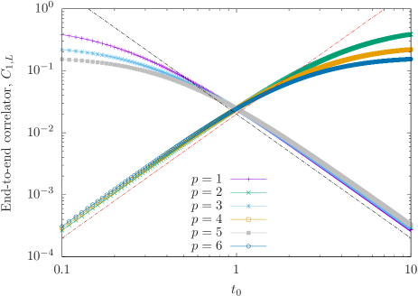
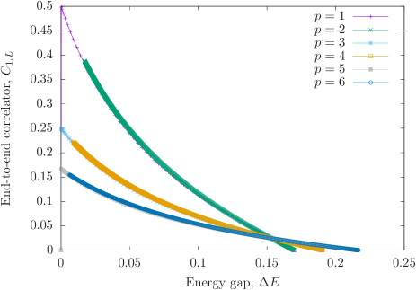
Figure 7: Edge-dimerized open boundary chains. Top: End-to-end correlation, $|C_{1,L}|$ as a function of the marked hopping, $t_{0}$, for $p=1$ to $6$, in logarithmic scale using $L=40$. The straight lines are power-laws corresponding to $t_{0}^{2}$ and $t_{0}^{-2}$. Bottom: End-to-end correlation, $|C_{1,L}|$ vs energy gap $\Delta E$ in all the previous cases. Notice the collapse of all the cases $p=2m-1$ and $p=2m$.

We would like to remark that the $t_{0}^{2}$ dependence can be heuristically justified assuming that the energy gap may be estimated via Eq. (14), despite the fact that the Dasgupta-Ma SDRG is not valid when the hoppings are not strongly inhomogeneous. In that case, the energy scale associated to the edge state is given by $t_{0}^{2}$. Of course, a rigorous justification is still missing.

The relation between the end-to-end correlation and the energy gap in the edge-dimerized chains is shown in the lower panel of Fig. 7. We see an interesting collapse of the values of $p$ by pairs: $\left\{1,2\right\}$, $\left\{3,4\right\}$ and $\left\{5,6\right\}$, i.e: cases $p=2m-1$ and $p=2m$ provide the same results.

Let us consider the entanglement structure of the edge-dimerized chains. Fig. 8 has a similar structure to that of Fig. 3. The top panel of Fig. 8 shows the entropy of blocks of the form $\left\{1,\cdots,\ell\right\}$ as a function of $\ell$, $S(\ell)$, for a chain with $L=64$ and different values of $t_{0}$. For $t_{0}=0$ the two extreme sites detach, while for $t_{0}=1$ we obtain the clean result, predicted by CFT, Eq. (18). As we increase $t_{0}$, the entropy becomes more flat, as in the bottom-right panel of Fig. 4, and a high peak is obtained for $S(2)$ and $S(L-2)$, denoting that the block $\left\{1,2\right\}$ cuts two bonds: the long distance bond $(1,L)$ and the short distance bond $(2,3)$. The central panel of Fig. 8 shows the half-chain entropy of the chain, $S(L/2)$ as a function of $t_{0}$ for different values of $L$ which form a geometric progression. The approximate arithmetic progression of the values denotes the logarithmic dependence of the entropy with the system size, typical of critical 1D systems, as opposed to the SSH case (Fig. 3, central). A relevant clue is provided by the entanglement contour of the left-half of the system with $L=64$, $s(i)$, plotted in the bottom panel of Fig. 8 for different values of $t_{0}$. Notice that the right extreme of the plot corresponds to the center of the chain. The curves for all values of $t_{0}$ are nearly identical, with a slight decrease of the bulk contour for large $t_{0}$, while there is a strong increase in the contour of first site, $s(1)$, which can be further noticed in the inset. This implies that the main effect of the increase of $t_{0}$ is just to create the edge state, the bond $(1,L)$, with a minimal distortion in the rest of the entanglement structure.

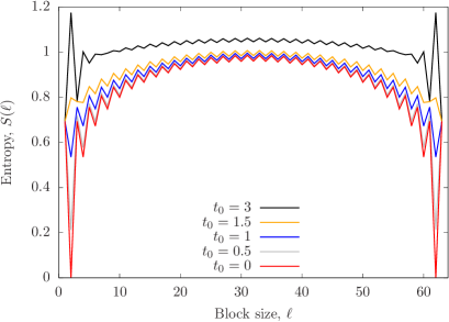
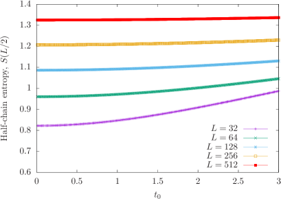
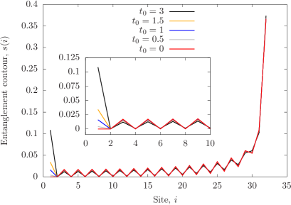
Figure 8: Entanglement structure of edge-dimerized states. Top: Entanglement entropy of blocks $\left\{1,\cdots,\ell\right\}$ as a function of the block size $\ell$ for different values of $t_{0}$, using $L=64$, on the GS of an edge-dimerized chain. Center: Half-system entanglement entropy $S(L/2)$ as a function of $t_{0}$, for different values of $L$. Notice the nearly flat behavior for large values of $L$. Bottom: entanglement contour for the left half of the $L=64$ system and the same values of $t_{0}$ used for the top panel. Inset: zoom on the left part of the block.

We have obtained that these edge-dimerized chains, with strong hopping amplitudes only in the second and penultimate links, give much better results for the large end-to-end correlations while maintaining a finite energy gap, a result that protects the edge state of the system making it quite robust.

Let us provide some numerical comparison. Consider the SSH chain, Eq. (1) with hoppings given in Eq. (15), using $L=40$ and $\delta=0.2$ gives an end-to-end correlation of $|C_{1,L}|\approx 0.3$, and an energy gap $\Delta E\approx 3.6\cdot 10^{-4}$. The same correlation can be obtained with an edge-dimerized chain (very close to the optimal case) using $t_{0}\approx 6.35$, for which the gap is now $\Delta E\approx 0.036$, i.e. 100 times larger. For larger values of $\delta$, the gap ratio can be even larger

VI Conclusions and further work

In this article we have explored 1D quantum systems in their ground states which, despite their local interactions, can develop large correlations between well separated sites (at the nanoscale). We have only considered independent fermions, but heuristic arguments suggest that similar structures could be found in presence of interactions. E.g. the rainbow state can be obtained in presence of a density-density repulsion Laguna.16 .

Open fermionic chains dimerize naturally in many relevant cases, due to the Peierls instability, thus giving rise to a SSH Hamiltonian. If the first and last hoppings are weak, a symmetry protected topological state is formed, characterized by the presence of an edge state which gives rise to very high end-to-end correlations. This edge-state can be explained using entanglement monogamy: all bulk sites pair up, leaving the first and last alone. Thus, a bond will be established between them. Nonetheless, Dasgupta-Ma renormalization arguments show that the energy gap associated with this state decreases faster than exponentially, leading to very low stability under external perturbations or a finite temperature.

We have developed a machine-learning algorithm in order to determine the hopping pattern which can give rise to the maximal possible end-to-end correlation for a given fixed energy gap on an open fermionic chain. The results show that modulated dimerizations, which are flat in the bulk, provide much better results. Optimality was usually achieved by patterns which present strong hopping amplitudes only in the second and penultimate links, which we have termed edge-dimerized chains.

The differences in robustness between the GS of the SSH model and the edge-dimerized one can be quite large: the energy gap can be more than 100 times larger for $L=40$ sites and a correlation of $0.3$ (being $0.5$ the maximal value, for a Bell pair). The differences in the entanglement structure are remarkable, and can help us understand the enhanced stability of the edge-dimerized Hamiltonian. Indeed, the entanglement entropy and contour show that the edge-dimerized GS is virtually identical to the clean one in the bulk, with a huge difference in the boundary. Thus, we can conjecture that the optimal correlation is mainly obtained by leaving the entanglement structure of the bulk untouched.

Of course, this stability can not be extended to arbitrarily large chains, but it can be used to engineer nanoscopic quantum systems with interesting properties comprising $\sim 50$-$100$ sites. Systems with these types of hopping patterns can appear naturally in quantum wires Ahn.03 ; Ahn.05 or organic molecules Gruner.88 , or can be engineered using optical lattices using the so-called cold-atom toolbox Lewenstein ; toolbox . On the other hand, spatial modulations of the hoppings have been proposed to study the effects of curved space-time on quantum matter and the Unruh effect Celi.10 ; Laguna_Celi.17 .

This work constitutes a proof-of-principle that edge-dimerization can help build strong long-distance correlations, along with some of the phenomena associated. Further relevant work will consider the applicability of these edge states for quantum information purposes, possible condensed-matter realizations, extension to more dimensions and dynamical effects.

- (1) L. Amico, R. Fazio, A. Osterloh, V. Vedral, Rev. Mod. Phys. 80, 517 (2008).
- (2) M.A. Nielsen, I.L. Chuang, Quantum computation and quantum information, Cambridge University Press (2000).
- (3) J. Eisert, M. Cramer, M.B. Plenio, Rev. Mod. Phys. 82, 277 (2010).
- (4) M. Srednicki, Phys. Rev. Lett. 71, 666 (1993).
- (5) G. Vidal, J.I. Latorre, E. Rico, A. Kitaev, Phys. Rev. Lett. 90, 227902 (2003).
- (6) G. Vitagliano, A. Riera, J.I. Latorre, New J. Phys. 12, 113049 (2010).
- (7) G. Ramírez, J. Rodríguez-Laguna, G. Sierra, J. Stat. Mech. P10004 (2014).
- (8) G. Ramírez, J. Rodríguez-Laguna, G. Sierra, J. Stat. Mech. P06002 (2015).
- (9) M.B. Hastings, J. Stat. Mech. P08024 (2007).
- (10) W. Su, J. Schrieffer, A. Heeger, Phys. Rev. Lett. 42, 1698 (1979).
- (11) A. Heeger, S. Kivelson, J. Schrieffer, W. Su, Rev. Mod. Phys. 60, 781 (1988).
- (12) J. Sirker, M. Maiti, N.P. Konstantinidis, N. Sedlmayr, J. Stat. Mech.: Theor. Exp., P10032 (2014).
- (13) J.K. Asbóth, L. Oroszlány, A. Pályi, A short course on topological insulators, Springer (2016).
- (14) I. Peschel, J. Phys. A: Math. Gen. 36, L205 (2003).
- (15) Y. Chen and G. Vidal, J. Stat. Mech. P10011 (2014).
- (16) E. Tonni, J. Rodríguez-Laguna, G. Sierra, J. Stat. Mech. 043105 (2018).
- (17) V. Alba, S.N. Santalla, P. Ruggiero, J. Rodríguez-Laguna, P. Calabrese, G. Sierra, ArXiv:1807.04179.
- (18) C. Dasgupta, S.K. Ma, Phys. Rev. B 22, 1305 (1980).
- (19) G. Ramírez, J. Rodríguez-Laguna, G. Sierra, J. Stat. Mech. P07003 (2014).
- (20) J. Rodríguez-Laguna, S.N. Santalla, G. Ramirez, G. Sierra, New J. Phys. 18, 073025 (2016).
- (21) J. Rodríguez-Laguna, J. Dubail, G. Ramirez, P. Calabrese, G. Sierra, J. Phys. A: Math. Theor. 50, 154001 (2017).
- (22) R. Peierls, Quantum theory of solids, Oxford University Press (1953).
- (23) R. Peierls, More suprises in theoretical physics, Princeton Series in Physics (1991).
- (24) P. C. Snijders, H. H. Weitering, Rev. Mod. Phys. 82, 307-329 (2010)
- (25) R. Grüner, Rev. Mod. Phys. 60, 1129-1181 (1988)
- (26) N. Sedlmayr, P. Jaeger, M. Maiti, J. Sirker, Phys. Rev. B 97, 064304 (2018).
- (27) J. Sirker, A. Herzog, A.M. Oleś, P. Horsch, Phys. Rev. Lett. 101, 157204 (2008).
- (28) P. Calabrese, J. Cardy, J. Stat. Mech. P06002 (2004).
- (29) P. Calabrese, J. Cardy, J. Phys. A: Math. Theor. 42, 504005 (2009).
- (30) J.C. Xavier, F.C. Alcaraz, Phys. Rev. B 83, 214425 (2011).
- (31) T. Weise, Global optimization algorithms –theory and application, www.it-weise.de/projects/book.pdf (2009).
- (32) A. Schrijver, A course on combinatorial optimization, homepages.cwi.nl/~lex/files/dict.pdf (2013).
- (33) G. Carleo, M. Troyer, Science 355, 602 (2017).
- (34) H. Fujita, Y.O. Nakagawa, S. Sugiura, M. Oshikawa Phys. Rev. B 97, 075114 (2018).
- (35) W.H. Press, S.A. Teukolsky, W.T. Vetterling, B.P. Flannery, Numerical Recipes: The art of scientific computing, Cambridge University Press (2007).
- (36) J. R. Ahn, P. G. Kang, K. D. Ryang, and H. W. Yeom, Phys. Rev. Letts. 95, 95, 196402, (2005).
- (37) J. R. Ahn, H. W. Yeom, H. S. Yoon, and I.- W. Lyo, Phys. Rev. Letts. 91, 196403 (2003).
- (38) M. Lewenstein, A. Sanpera, V. Ahufinger, Ultracold atoms in optical lattices, Oxford University Press (2012).
- (39) D. Jaksch, P. Zoller, Ann. Phys. 315, 52 (2005).
- (40) O. Boada, A. Celi, J.I. Latorre, M. Lewenstein, New J. Phys. 13, 035002 (2010).
- (41) J. Rodríguez-Laguna, L. Tarruell, M. Lewenstein, A. Celi, Phys. Rev. A 95, 013627 (2017).