Relative Resolution:

A Multipole Approximation
at Appropriate Distances

Abstract

Recently, we introduced Relative Resolution as a hybrid formalism for fluid mixtures [1]. The essence of this approach is that it switches molecular resolution in terms or relative separation: While nearest neighbors are characterized by a detailed fine-grained model, other neighbors are characterized by a simplified coarse-grained model. Once the two models are analytically connected with each other via energy conservation, Relative Resolution can capture the structural and thermal behavior of (nonpolar) multi-component and multi-phase systems across state space. The current work is a natural continuation of our original communication [1]. Most importantly, we present the comprehensive mathematics of Relative Resolution, basically casting it as a multipole approximation at appropriate distances; the current set of equations importantly applies for all systems (e.g, polar molecules). Besides, we continue examining the capability of our multiscale approach in molecular simulations, importantly showing that we can successfully retrieve not just the statics but also the dynamics of liquid systems. We finally conclude by discussing how Relative Resolution is the inherent variant of the famous “cell-multipole” approach for molecular simulations.

1 Introduction

Over the past half of a century, invoking molecular simulations has become one of the most promising routes for studying soft matter. This computational approach is splendid for describing systems that just comprise small spatial and short temporal dimensions (i.e., $<10^{-6}$m and $<10^{-6}$s, respectively), but it is deficient in describing systems that also involve large spatial and long temporal dimensions (i.e., $>10^{-3}$m and $>10^{-3}$s, respectively); resolving such challenges is especially important for biological processes, whose particularities usually span orders of magnitude in scale. For overcoming this dimensionality issue, special attention has been given for enhancing the computational efficiency of molecular simulations, while ensuring that the phenomena of interest is still correctly retrieved. One route involves the intelligent use of statistical mechanics while designing sophisticated algorithms. For example, various successful strategies have been developed that focus on improving the computational efficiency of specific aspects of molecular simulations (e.g., free energies [2, 3, 4, 5], reaction coefficients [6, 7, 8, 9], etc.).

Our work revolves around another set of algorithms that has received much attention in the recent couple of decades: It is commonly called the multiscale approach, and it generally takes on the in-serial or in-parallel format. Rather than focusing on the calculation of a specific feature of a molecular simulation, multiscale algorithms aim at improving the computational efficiency of the entire system, while ideally capturing all of its static and dynamic behavior. Importantly, the main signature of all multiscale simulations is that they involve two systems, one constructed of detailed Fine-Grained (FG) models with many degrees of freedom (usually corresponding with atomistic coordinates), and one constructed of simplified Coarse-Grained (CG) models with few degrees of freedom (usually corresponding with gravitational centers). While many multiscale strategies exist that combine quantum-classical descriptions and discrete-continuum descriptions, the focus of our publication is on algorithms that combine FG and CG molecular models based on Newtonian particles.

The in-serial multiscale methods generally focus on the FG and CG systems in successive order: In the usual case, they begin by postulating a particular set of FG models, and after performing a sufficient amount of molecular simulations of this detailed system, they optimize, based on a certain criterion, a respective set of CG models, continuing the remainder of their investigation only with molecular simulations of this simplified system. While in practice, there are many variants of this type of multiscale strategies [10, 11], each of these can be derived via one of two comprehensive frameworks: One stems in the relative entropy [12], while the other aims at “force-matching” [13, 14]. The former multiscale approach minimizes a functional which measures the logarithmic ratios between the FG and CG configurational probabilities [12], and it has been shown that the relative entropy underlies the uniqueness theorem of Henderson [15], which is the basis for various strategies that focus on capturing radial distributions between molecular pairs [16, 17, 18, 19]. The latter multiscale approach minimizes a functional which measures the squared differences between the FG and CG instantaneous forces, and it is has been shown that that “force-matching” is equivalent with a generalized version of the Yvon-Born-Green formalism [20]. Besides, both of these formalisms retrieve the famous multi-body potential of Kirkwood [21].

While all of the in-serial multiscale methods have achieved much success, they still have several unresolved issues. On a fundamental level, it is agreed upon that no model can optimally transfer across state space (e.g., across temperature and density), while also concurrently representing all structural correlations and thermal properties of a given system [22, 23]. This technically means that one must choose a particular aspect of the molecular system for optimization (e.g., a configurational probability or an instantaneous force), while having no guarantee of replicating any of its other behavior, and on top of this, this protocol must be repetitively performed at each state point of interest. Furthermore on a very practical level, the most significant challenge with all of these multiscale strategies is the fact that a very undesirable computational step is always required: This step involves performing a molecular simulation of a particular FG model before even using a respective CG model; realize that in general, if we can construct a molecular simulation of the former, we do not really need the latter. Finally, we note that because of the reduction in the degrees of freedom, time-scales naturally change during multiscale optimization, and thus, kinetic features will inherently deviate from their true behavior.

The in-parallel multiscale methods generally contain FG and CG information simultaneously in a unified system: A single molecular simulation contains both FG and CG models, with vital aspects described in detail by the latter, and trivial aspects described with simplicity by the former. Diverse strategies have been developed that follow this hybrid computational path, and we categorize them here in four main classes. The most straightforward approach is the “group-based” multiscale method: Here, essential molecular groups (e.g., solute molecules) are described via FG interactions, and auxiliary molecular groups (e.g., solvent molecules) are described via CG interactions [24, 25, 26, 27]. The next class of strategies can be thought of as the “time-based” multiscale method: A given molecular simulation spends some of its time as the FG system and some of its time as the CG system, with the results being recorded for the former and discarded for the latter [28, 29]. A powerful variation of this approach actually exchanges among FG and CG replicas of the molecular simulation, which enhances the overall efficiency of the computational procedure [30, 31]. In either case, this hybrid approach is obviously convenient for overcoming various time-scale barriers in a system of interest.

Perhaps the most successful class of the in-parallel multiscale methods has been the one which is commonly called Adaptive Resolution. With much research done on it for over a decade, this approach is a “one-body distance-based” multiscale method: In a single molecular simulation, adaptive molecules switch their resolution in terms of absolute position [32, 33, 34, 35]. For example, as molecules move around a system, they adopt a FG model if near to the origin and a CG model if far from the origin. In practice, Adaptive Resolution essentially constructs hybrid molecules that embody both FG and CG models, and in fact, the main difference between all variations of Adaptive Resolution has been the mixing rule for the hybrid interaction as a function of absolute position. In the original publication for Adaptive Resolution, Praprotnik et al. introduced the hybrid interaction as a linear combination of forces, and this has been the ideal choice for evolving Newtonian trajectories [32]; in that same journal issue, Abrams presented an alternative route that switches between the models in a stochastic manner [33]. Conversely, Ensing et al. formulated the hybrid interaction as a linear combination of potentials [34]; in turn, Potestio et al. showed that such a Hamiltonian version of Adaptive Resolution naturally corresponds with many aspects in statistical mechanics [35]. On a practical level, Adaptive Resolution is especially useful if a given system has a specific region of special interest (e.g., a protein at the origin, with everything else being water). As such, Adaptive Resolution has been already applied in some biological scenarios, having quite successful results [36, 37].

Very recently, we developed another type of multiscale methods, termed Relative Resolution (RelRes) [1]. Inspired by Adaptive Resolution, this approach is a “two-body distance-based” multiscale method: In a single molecular simulation, hybrid molecules switch their resolution in terms of relative separation; in particular, molecules that are near neighbors (i.e., their pairwise distance is small) interact via their FG models, and molecules that are far neighbors (i.e., their pairwise distance is large) interact via their CG models [1]. Importantly, RelRes is the sole class of multiscale simulations which describes all molecules, for all times, with both FG and CG models; the resolution of a given molecule is always relative of its observer. While other strategies, reminiscent of RelRes, have been also developed [38, 39], our formalism is unique in that it mathematically finds a natural connection between the FG and CG potentials. While Ref. [38] numerically parametrizes between the two models via “force-matching”, Ref. [39] does not make a clear connection between the two models. Conversely, we developed an analytical parameterization between the FG and CG models, which is just based on energy conservation [1]. Unlike those other strategies [38, 39], we were consequently able of correctly retrieving across state space, the structural and thermal behavior of several nonpolar mixtures [1]. Besides, we showed that our hybrid approach can be considered as a generalized extension of established theories for uniform liquids, which assume a mean field for interactions beyond a certain distance [40, 41, 42, 43].

In this current work, we build on our original communication of RelRes [1]. Foremost, we mathematically present the comprehensive framework for RelRes. Above all by performing a multipole expansion for an arbitrary potential of inverse powers, we show that its zero-order term, which is sufficient for nonpolar systems, is identical with the succinct expression we presented in our initial publication; in consideration of polar systems, the current work also presents the first-order and second-order terms of the Taylor series, both of which involve molecular orientation. By use of this multipole approximation, we introduce RelRes as a Hamiltonian that switches between the FG and CG models at an appropriate distance. Building on the computational results of our original work, we consequently continue examining RelRes with molecular simulations of nonpolar systems. Interestingly, we find that the ideal switching distance between the FG and CG models is roughly equivalent with the location at which a particular orientational function essentially decorrelates. Besides, we also demonstrate that RelRes can correctly describe not just static behavior but also dynamic behavior. Together with our previous publication [1], we suggest that RelRes can be a powerful multiscale tool for efficiently studying soft matter via molecular simulations.

2 Theoretical Foundation

Contrary to our original publication [1], we present here our hybrid formalism in a reversed order. In the previous work, we started by defining RelRes, and we ended by parameterizing between the FG and CG potentials. In the current work, we start by parameterizing between the FG and CG potentials, and we end by defining RelRes. Regardless, the mathematical notation is identical between our two publications. Note also that the current framework is the comprehensive one, applying for all molecular systems. The original publication is the terse version, which is only applicable for nonpolar scenarios.

2.1 Defining our System

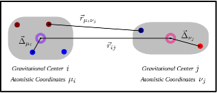
Figure 1: A pair of molecules in vacuum. The gravitational centers are represented by hollow rings, and the atomistic coordinates are represented by replete disks. The left side is for molecule $i$ with its $\mu_{i}$ sites, and the right side is for molecule $j$ with its $\nu_{j}$ sites. The various colors of these mean that they can all be inherently different in terms of their interaction parameters. The gray shading does not have much of a physical meaning: It just helps us delineate the approximate boundary of a molecule. The various arrows are distance vectors. $\overrightarrow{r}_{ij}$ is the distance between centers $i$ and $j$, and $\vec{r}_{\mu_{i}\nu_{j}}$ is the distance between coordinates $\mu_{i}$ and $\nu_{j}$. Within each molecule, $\overrightarrow{\Delta}_{\mu_{i}}$ or $\overrightarrow{\Delta}_{\nu_{j}}$ is a vector between an atomistic coordinate, $\mu_{i}$ or $\nu_{j}$, and a gravitational center, $i$ or $j$, respectively.

Consider that we are performing a molecular simulation of a pair of molecules in vacuum; a particular configuration of this trivial system is depicted in Fig. 1. We label the gravitational centers by the Latin indices $i$ and $j$, and we label the atomistic coordinates by the Greek indices $\mu$ and $\nu$. In our notation throughout, we denote $n_{i}$ or $n_{j}$ as the number of sites on a molecule $i$ or $j$, respectively. The relative separation between the centers is $\overrightarrow{r}_{ij}$, and the relative separation between the coordinates is$\overrightarrow{r}_{\mu_{i}\nu_{j}}$. Furthermore, the distance between a certain atomistic coordinate and a respective gravitational center is $\overrightarrow{\Delta}_{\mu_{i}}$ or $\overrightarrow{\Delta}_{\nu_{j}}$. By Fig. 1, it is clear that these distances are related as follows,

$$\overrightarrow{\Delta}_{\mu_{i}\nu_{j}}=\overrightarrow{r}_{\mu_{i}\nu_{j}}-\overrightarrow{r}_{ij}$$ (1)

and we defined in this expression the following variable:

$$\overrightarrow{\Delta}_{\mu_{i}\nu_{j}}=\overrightarrow{\Delta}_{\nu_{j}}-\overrightarrow{\Delta}_{\mu_{i}}$$ (2)

Note that we introduce here all distances in vector form, and their scalar definitions naturally follow. We also define dimensionless variables that will compact all of our ensuing mathematics:

$$\overrightarrow{\xi}_{\mu_{i}\nu_{j}}=\frac{\overrightarrow{\Delta}_{\mu_{i}\nu_{j}}}{r_{ij}}$$ (3)

$$\cos\theta_{\mu_{i}\nu_{j}}=\frac{\overrightarrow{r}_{ij}\cdot\overrightarrow{\Delta}_{\mu_{i}\nu_{j}}}{r_{ij}\Delta_{\mu_{i}\nu_{j}}}$$ (4)

With these definitions, together with some rearrangement, we attain this useful relation which basically stems in the dot product of Eq. 1 with itself:

$$\frac{r_{\mu_{i}\nu_{j}}}{r_{ij}}=\sqrt{1+2\xi_{\mu_{i}\nu_{j}}\cos\theta_{\mu_{i}\nu_{j}}+\xi_{\mu_{i}\nu_{j}}^{2}}$$ (5)

Finally for clarity, we must make a subtle distinction with a variable, $\Delta r_{\mu_{i}\nu_{j}}$, that appears in our original communication, but that we do not use here: $\Delta r_{\mu_{i}\nu_{j}}=r_{\mu_{i}\nu_{j}}-r_{ij}\neq\Delta{}_{\mu_{i}\nu_{j}}$.

We now focus on the energetics of this rudimentary system. The governing function here is defined as follows:

$$u_{ij}\left(\overrightarrow{r}_{ij};\left\{\overrightarrow{\Delta}_{\mu_{i}}\right\},\left\{\overrightarrow{\Delta}_{\nu_{j}}\right\}\right)=\sum_{\mu_{i}\nu_{j}}{\displaystyle u_{\mu_{i}\nu_{j}}\left(r_{\mu_{i}\nu_{j}}\right)}$$ (6)

Here, $u_{\mu_{i}\nu_{j}}$ is the intrinsic potential between atomistic coordinates $\mu_{i}$ and $\nu_{j}$, and $u_{ij}$ is the resultant potential between gravitational centers $i$ and $j$; the latter is obtained by the respective summation of the former. Notice that we are allowing for absolute nonuniformity in our mixtures considering the indices on the potentials, $u_{\mu_{i}\nu_{j}}$ and $u_{ij}$. Importantly, we assume that the former is isotropic, being exclusively a function of the scalar $r_{\mu_{i}\nu_{j}}$. Conversely, we expect that the latter is geometric, being chiefly a function of the vector $\overrightarrow{r}_{ij}$, as well as the two sets of intramolecular distances, $\left\{\overrightarrow{\Delta}_{\mu_{i}}\right\}$ and $\left\{\overrightarrow{\Delta}_{\nu_{j}}\right\}$. Importantly, we ignore intramolecular energetics during most of our derivation: These are accounted for once we present the entire Hamiltonian of RelRes.

One of the focal assumptions in our analysis is that the basis function of the potential can be cast as an inverse power of the isotropic distance:

$$u_{\mu_{i}\nu_{j}}\left(r\right)=\frac{c_{\mu_{i}\nu_{j}}}{r^{m}}$$ (7)

Obviously, $m$ is the power associated with this inverse law. In most scenarios, like with the Coulomb potential ($m=1$), as well as with the Lennard-Jones (LJ) potential ($m=12$ and $m=6$), the inverse law is a natural choice. The proportionality coefficient $c_{\mu_{i}\nu_{j}}$ corresponds with the unique parameters involved in the interaction between sites $\mu_{i}$ and $\nu_{j}$, and it is usually known empirically for use in molecular simulations. We will later make an important assumption of geometric mixing for $c_{\mu_{i}\nu_{j}}$ (i.e., we will express it as a product of two separate parameters).

In the remainder of the derivation, our goal is to reformulate $u_{ij}$ of Eq. 6 in terms of $r_{ij}$, together with variations of $\overrightarrow{\xi}_{\mu_{i}\nu_{j}}$ and $\cos\theta_{\mu_{i}\nu_{j}}$, as defined by Eqs. 3 and 4. Such a reformulation holds a promise for the efficient calculation of the energy of the pair in Fig. 1; obviously, computation of a single distance, $r_{ij}$, is preferable over the computation of $n_{i}n_{j}$ distances, $r_{\mu_{i}\nu_{j}}$, which the summation of Eq. 6 requires. Of course, such a reformulation may involve approximations, and thus, we must make valid assumptions for $\overrightarrow{\xi}_{\mu_{i}\nu_{j}}$ and $\cos\theta_{\mu_{i}\nu_{j}}$ so that we maintain the correct energy for this pair.

2.2 Introducing the Multipole Expansion

We substitute Eq. 7 in Eq. 6, which yields the following:

$$u_{ij}\left(\overrightarrow{r}_{ij};\overrightarrow{\xi}_{\mu_{i}\nu_{j}},\cos\theta_{\mu_{i}\nu_{j}}\right)=\sum_{\mu_{i}\nu_{j}}\frac{c_{\mu_{i}\nu_{j}}}{r_{\mu_{i}\nu_{j}}^{m}}$$ (8)

For clarity throughout most of the ensuing analysis, $\overrightarrow{\xi}_{\mu_{i}\nu_{j}}$ and $\cos\theta_{\mu_{i}\nu_{j}}$ are omitted yet implied in the functionalities involved in Eq. 8; the same also goes for the bar on $\overrightarrow{r}_{ij}$. Consider now the radial distance which appears here together with the power of $m$; we correspondingly exponentiate Eq. 5, and we present the ensuing reciprocal:

$$\left(\frac{r_{ij}}{r_{\mu_{i}\nu_{j}}}\right)^{m}=\left(1+2\xi_{\mu_{i}\nu_{j}}\cos\theta_{\mu_{i}\nu_{j}}+\xi_{\mu_{i}\nu_{j}}^{2}\right)^{-m/2}$$ (9)

We can use this expression to substitute the computationally inexpensive $r_{ij}$ for the computationally expensive $r_{\mu_{i}\nu_{j}}$ in Eq. 8. We consequently attain the following expression:

$$u_{ij}\left(r_{ij}\right)=\frac{1}{r_{ij}^{m}}\sum_{\mu_{i}\nu_{j}}\left[c_{\mu_{i}\nu_{j}}\cdot\left(1+2\xi_{\mu_{i}\nu_{j}}\cos\theta_{\mu_{i}\nu_{j}}+\xi_{\mu_{i}\nu_{j}}^{2}\right)^{-m/2}\right]$$ (10)

Analogous with the usual multipole expansion, we now reformulate, via a Taylor series, the cumbersome expression which appears above,

$$\left(1+2\xi\cos\theta+\xi^{2}\right)^{-m/2}=\sum_{\aleph}\left[\Lambda_{m,\aleph}\left(\cos\theta\right)\cdot\xi^{\aleph}\right]$$ (11)

with $\Lambda_{m,\aleph}$ basically defined by the appropriate derivative in terms of the index $\aleph$:

$$\Lambda_{m,\aleph}\left(\cos\theta\right)=\frac{1}{\aleph!}\left[\frac{\partial^{\aleph}}{\partial\xi^{\aleph}}\left(1+2\xi\cos\theta+\xi^{2}\right)^{-m/2}\right]_{\xi=0}$$ (12)

Clearly, $\Lambda_{m,\aleph}$ is only a function of $\cos\theta_{\mu_{i}\nu_{j}}$, with the functionality of $\xi_{\mu_{i}\nu_{j}}$ appearing as a power in Eq. 11. Realize that such a Taylor expansion is justified by the fact that usually, $\xi_{\mu_{i}\nu_{j}}<1$ (i.e., $\Delta_{\mu_{i}\nu_{j}}<r_{ij}$), since in most cases, bonds are negligible in magnitude compared with intermolecular distances. Notice also that the exponent $m$ of the inverse law is just a parameter in $\Lambda_{m,\aleph}$. Besides, if $m=1$ (i.e., the Coulomb potential), Eq. 11 simply becomes the common definition of the Legendre polynomials.

Substituting Eq. 11 in Eq. 10 yields the following power series for our energy function:

$$u_{ij}\left(r_{ij}\right)=\frac{1}{r_{ij}^{m}}\sum_{\aleph}\left[\sum_{\mu_{i}\nu_{j}}\left[c_{\mu_{i}\nu_{j}}\Lambda_{m,\aleph}\left(\cos\theta_{\mu_{i}\nu_{j}}\right)\xi_{\mu_{i}\nu_{j}}^{\aleph}\right]\right]$$ (13)

and it is particularly convenient to cast the above as follows,

$$u_{ij}\left(r_{ij}\right)=\frac{1}{r_{ij}^{m}}\sum_{\aleph}c_{ij,\aleph}\left(\xi_{\mu_{i}\nu_{j}},\cos\theta_{\mu_{i}\nu_{j}}\right)$$ (14)

in which we obviously defined the following:

$$c_{ij,\aleph}\left(\xi_{\mu_{i}\nu_{j}},\cos\theta_{\mu_{i}\nu_{j}}\right)=\sum_{\mu_{i}\nu_{j}}\left[c_{\mu_{i}\nu_{j}}\Lambda_{m,\aleph}\left(\cos\theta_{\mu_{i}\nu_{j}}\right)\xi_{\mu_{i}\nu_{j}}^{\aleph}\right]$$ (15)

One may think of $c_{ij,\aleph}$ as an effective coefficient for a given configuration of Fig. 1; analogous with $u_{ij}$, $\xi_{\mu_{i}\nu_{j}}$ and $\cos\theta_{\mu_{i}\nu_{j}}$ are consequently omitted yet implied in the functionality of $c_{ij,\aleph}$ throughout most of our derivation. In any case, notice that these expressions are especially useful for computational purposes: By summing over all sites $\mu_{i}$ and $\nu_{j}$, one can separately calculate the energetic coefficient of any $\aleph$ term by Eq. 15, and by including as many $\aleph$ terms in Eq. 14 as desired, one can have a valid approximation for the overall interaction between the molecular pair of Fig. 1. Of particular importance is the leading (nonvanishing) $\aleph$ term: For making a connection with the terminology of the original work, we term it as the Molecular Pair in the Infinite Limit (MPIL).

2.3 Evaluating the Multipole Terms

By not even performing any differentiation, the $\aleph=0$ term is readily determined by Eq. 12 as the following:

$$\Lambda_{m,0}=1$$ (16)

Conveniently, this is always unity, regardless of the value of $m$. Plugging this in Eq. 15, we attain this expression:

$$c_{ij,0}=\sum_{\mu_{i}\nu_{j}}c_{\mu_{i}\nu_{j}}$$ (17)

Notice here that this is not dependent at all on the configuration of the molecular pair: This means $c_{ij,0}$ is a constant that can be calculated before any molecular simulation is performed. If this is nonzero, we can approximate our energy in Eq. 14:

$$u_{ij}\left(r_{ij}\right)\approx\frac{c_{ij,0}}{r_{ij}^{m}}$$ (18)

$$u_{ij}\left(r_{ij}\right)\approx\frac{\sum_{\mu_{i}\nu_{j}}c_{\mu_{i}\nu_{j}}}{r_{ij}^{m}}$$

In the later part of this expression, we obviously invoked Eq. 17. Notice the similarity between Eqs. 8 and 18: We start with an $m$ inverse law in the former, and we end with an $m$ inverse law in the latter. In Eq. 8, we sum over the many distances between the atomistic coordinates, with their intrinsic interaction coefficients, and in Eq. 18, we take in the single distance between the gravitational centers, with its resultant interaction coefficient. This is in effect the monopole term; once we introduce another assumption, we will show that this is specifically equivalent with the monopole-monopole interaction.

This is in essence the sole term that we derived in our previous work. We simply attained it by vanishing all bond lengths (i.e., $\Delta_{\mu_{i}\nu_{j}}=0$) in Fig. 1; this is basically equivalent to setting all $\xi_{\mu_{i}\nu_{j}}=0$ in Eq. 10, and in turn, it also eliminates the corresponding functionality of all $\cos\theta_{\mu_{i}\nu_{j}}$ in our energy expression. The only discrepancy of Eq. 18 with the corresponding one in our original work is that in this one, we have the assumption of the inverse power for the interaction. We can remove this assumption temporarily by invoking Eq. 7 for Eq. 18, and we in turn get the exact expression which we termed as the MPIL in our original publication:

$$u_{ij}\left(r_{ij}\right)\approx\sum_{\mu_{i}\nu_{j}}u_{\mu_{i}\nu_{j}}\left(r_{ij}\right)$$ (19)

Realize that that this is a special case of our current definition of the MPIL: As mentioned before, the general definition of our MPIL is the leading (nonvanishing) $\aleph$ term in Eq. 13.

Importantly in our original work, we showed that if Eq. 18 is implemented with RelRes, it can successfully describe nonpolar mixtures that are based on the LJ potential. Theoretically, this approximation shall also work with the Coulomb potential for ionic molecules that have a net charge. In fact for RelRes, we expect that Eq. 18 shall be adequate for any $m$, given that this monopole term does not vanish. Nevertheless, once the above summation for a certain molecular pair contains both positive and negative values for $c_{\mu_{i}\nu_{j}}$, there may be some issues; specifically, if all $c_{\mu_{i}\nu_{j}}$ in the summation cancel each other, Eq. 18 is strictly zero. The most obvious such case is the zwitterionic scenario, in which the molecules have Coulombic charges, yet they are overall neutral (e.g., water). It is obvious that the interaction between such polar pairs is finite, and consequently, one must go beyond the monopole term of Eq. 18 in order to describe the corresponding energy, at least approximately. This is in fact the purpose of the ensuing mathematics. Note that the equations below may be also useful as correction terms for the interaction between the molecular pair, even if their monopole term is nonzero.

Obviously, all the terms of the Taylor series can be evaluated by successive differentiation as presented in Eq. 12. Here is the first-order term:

$$\Lambda_{m,1}\left(\cos\theta\right)=\left[m\left(\cos\theta+\xi\right)\left(1+2\xi\cos\theta+\xi^{2}\right)^{-\left(m+2\right)/2}\right]_{\xi=0}$$

$$\Lambda_{m,1}\left(\cos\theta\right)=m\cos\theta$$ (20)

Consequently, the $\aleph=1$ term of Eq. 15 is the following,

$$c_{ij,1}\left(\xi_{\mu_{i}\nu_{j}},\cos\theta_{\mu_{i}\nu_{j}}\right)=m\sum_{\mu_{i}\nu_{j}}\left[c_{\mu_{i}\nu_{j}}\cos\theta_{\mu_{i}\nu_{j}}\xi_{\mu_{i}\nu_{j}}\right]$$ (21)

Here is the second-order term:

$$\Lambda_{m,2}\left(\cos\theta\right)=\frac{1}{2}\left[m\left(m+2\right)\left(\cos\theta+\xi\right)^{2}\left(1+2\xi\cos\theta+\xi^{2}\right)^{-\left(m+4\right)/2}-m\left(1+2\xi\cos\theta+\xi^{2}\right)^{-\left(m+2\right)/2}\right]_{\xi=0}$$

$$\Lambda_{m,2}\left(\cos\theta\right)=\frac{m}{2}\left(\left(m+2\right)\cos^{2}\theta-1\right)$$ (22)

Consequently, the $\aleph=2$ term of Eq. 15 is the following,

$$c_{ij,2^{+}}\left(\xi_{\mu_{i}\nu_{j}},\cos\theta_{\mu_{i}\nu_{j}}\right)=\frac{m}{2}\sum_{\mu_{i}\nu_{j}}\left[c_{\mu_{i}\nu_{j}}\cos^{2}\theta_{\mu_{i}\nu_{j}}\xi_{\mu_{i}\nu_{j}}^{2}\right]$$ (23)

$$c_{ij,2^{-}}\left(\xi_{\mu_{i}\nu_{j}},\cos\theta_{\mu_{i}\nu_{j}}\right)=\frac{m}{2}\sum_{\mu_{i}\nu_{j}}\left[c_{\mu_{i}\nu_{j}}\xi_{\mu_{i}\nu_{j}}^{2}\right]$$ (24)

Here, we introduced this definition:

$$c_{ij,2}\left(\xi_{\mu_{i}\nu_{j}},\cos\theta_{\mu_{i}\nu_{j}}\right)=\left(m+2\right)c_{ij,2^{+}}-c_{ij,2^{-}}$$ (25)

We also emphasize here that if $m=1$ (e.g., the Coulombic scenario), $\Lambda_{m,1}$ and $\Lambda_{m,2}$ become the familiar first and second Legendre polynomials, respectively.

Of course, these $c_{ij,\aleph}$ can be readily used for evaluating the energy function of Eq. 14: They may serve as correction terms for Eq. 18, and if $c_{ij,1}$ or $c_{ij,2}$ is actually the leading term of this multipole expansion, it can even become the sole approximation for the energy (i.e., the MPIL). Notice that unlike $c_{ij,0}$, these current expressions are functions of $\cos\theta_{\mu_{i}\nu_{j}}$, and well as $\xi_{\mu_{i}\nu_{j}}$. Thus, while Eq. 18 is isotropic, involving just the scalar $r_{ij}$ in its functionality, the energy which corresponds with other $c_{ij,\aleph}$ is geometric, involving also the vector $\overrightarrow{\Delta}_{\mu_{i}\nu_{j}}$ in its functionality. Thus for $\aleph\neq 0$, the coefficient must be computed at each step of a molecular simulation. As such, going beyond the monopole term obviously requires significant computational cost, and it is only recommended if it is necessary (i.e., for polar systems in which these are the leading terms in the Taylor series).

2.4 Assuming a Proportionality Coefficient

Let us now discuss the proportionality coefficient $c_{\mu_{i}\nu_{j}}$ of the inverse law of Eq. 7. In most cases, such a parameter is empirically known for use in molecular simulations. In fact, it is usually expressed in terms of some mixing rules between two separate coefficients $\mathfrak{c}_{\mu_{i}}$ and $\mathfrak{c}_{\nu_{j}}$ of sites $\mu_{i}$ and $\nu_{j}$, respectively. For example with the Coulomb potential, $c_{\mu_{i}\nu_{j}}$ is fundamentally the product of partial charges; an analogous product is also sometimes used for the LJ potential. For the remainder of our work, we assume that the following equation holds:

$$c_{\mu_{i}\nu_{j}}=\mathfrak{c}_{\mu_{i}}\mathfrak{c}_{\nu_{j}}$$ (26)

For completeness, this means that Eq. 8 (i.e., the initial energy function in our derivation that introduced the inverse power), becomes the following:

$$u_{ij}\left(\overrightarrow{r}_{ij};\overrightarrow{\xi}_{\mu_{i}\nu_{j}},\cos\theta_{\mu_{i}\nu_{j}}\right)=\sum_{\mu_{i}\nu_{j}}\frac{\mathfrak{c}_{\mu_{i}}\mathfrak{c}_{\nu_{j}}}{r_{\mu_{i}\nu_{j}}^{m}}$$ (27)

In any case, Eq. 26 substantially facilitates our computational algorithm for RelRes, especially since a variant of $c_{ij,\aleph}$, for any $\aleph$, becomes a constant during a molecular simulation.

Let us begin with the zero-order term. Substituting Eq. 26 in Eq. 17, we attain the following equation

$$c_{ij,0}=\mathfrak{c}_{i,0}\mathfrak{c}_{j,0}$$ (28)

in which we have introduced the definition of the monopole $\mathfrak{c}_{i,0}$ or $\mathfrak{c}_{j,0}$, for each molecule $i$ or $j$, respectively:

$$\begin{array}[]{c}\mathfrak{c}_{i,0}=\sum_{\mu_{i}}\mathfrak{c}_{\mu_{i}}\\ \mathfrak{c}_{j,0}=\sum_{\nu_{j}}\mathfrak{c}_{\nu_{j}}\end{array}$$ (29)

If both of these monopoles are nonzero, the MPIL is the following according to Eq. 14:

$$u_{ij}\left(r_{ij}\right)\approx\frac{\mathfrak{c}_{i,0}\mathfrak{c}_{j,0}}{r_{ij}^{m}}$$ (30)

$$u_{ij}\left(r_{ij}\right)\approx\frac{\left(\sum_{\mu_{i}}\mathfrak{c}_{\mu_{i}}\right)\left(\sum_{\nu_{j}}\mathfrak{c}_{\nu_{j}}\right)}{r_{ij}^{m}}$$

Analogous with our comparison of Eqs. 8 and 18 above, notice the similarity between Eqs. 27 and 30: Performing the approximation, we start with several inverse coefficients $\mathfrak{c}_{\mu_{i}}\mathfrak{c}_{\nu_{j}}$, and we end with one inverse coefficient $\mathfrak{c}_{i,0}\mathfrak{c}_{j,0}$.

We now consider the benefit of the product assumption of Eq. 26. You may notice that Eq. 30 may be slightly more computationally efficient than Eq. 18. The former involves two summations over $n_{i}$ and $n_{j}$ parameters, while the latter involves one summation over $n_{i}n_{j}$ parameters. Regardless, all of these summations can be performed before a molecular simulation, and thus, they have negligible computational cost. The computational superiority introduced via Eq. 26 becomes very apparent once we move to the first-order and second-order terms of the multipole expansion.

We may now apply the assumption of Eq. 26 for evaluating any $c_{ij,\aleph}$, as presented in Eq. 15, after the appropriate differentiation of Eq. 12. As an important part of the ensuing mathematics, we introduce the familiar definition for the dipole $\overrightarrow{\mathfrak{p}}_{i,1}$ or $\overrightarrow{\mathfrak{p}}_{j,1}$, of each molecule $i$ or $j$, respectively:

$$\begin{array}[]{c}\overrightarrow{\mathfrak{p}}_{i,1}=\sum_{\mu_{i}}\left[\mathfrak{c}_{\mu_{i}}\overrightarrow{\Delta}_{\mu_{i}}\right]\\ \overrightarrow{\mathfrak{p}}_{j,1}=\sum_{\nu_{j}}\left[\mathfrak{c}_{\nu_{j}}\overrightarrow{\Delta}_{\nu_{j}}\right]\end{array}$$ (31)

Moreover, we introduce components of the familiar definition for the quadrupole $\left(\overrightarrow{\overrightarrow{\mathfrak{q}}}_{i,2},\mathfrak{q}_{i,0}\right)$ or $\left(\overrightarrow{\overrightarrow{\mathfrak{q}}}_{j,2},\mathfrak{q}_{j,0}\right)$, of each molecule $i$ or $j$, respectively:

$$\begin{array}[]{c}\overrightarrow{\overrightarrow{\mathfrak{q}}}_{i,2}=\sum_{\mu_{i}}\left[\mathfrak{c}_{\mu_{i}}\overrightarrow{\Delta}_{\mu_{i}}\overrightarrow{\Delta}_{\mu_{i}}\right]\\ \overrightarrow{\overrightarrow{\mathfrak{q}}}_{j,2}=\sum_{\nu_{j}}\left[\mathfrak{c}_{\nu_{j}}\overrightarrow{\Delta}_{\nu_{j}}\overrightarrow{\Delta}_{\nu_{j}}\right]\end{array}$$ (32)

$$\begin{array}[]{c}\mathfrak{q}_{i,0}=\sum_{\mu_{i}}\left[\mathfrak{c}_{\mu_{i}}\Delta_{\mu_{i}}^{2}\right]\\ \mathfrak{q}_{j,0}=\sum_{\nu_{j}}\left[\mathfrak{c}_{\nu_{j}}\Delta_{\nu_{j}}^{2}\right]\end{array}$$ (33)

By casting a linear combination of these, $\left(m+2\right)\overrightarrow{\overrightarrow{\mathfrak{q}}}_{i,2}-\mathfrak{q}_{i,0}\overrightarrow{\overrightarrow{\delta}}$ or $\left(m+2\right)\overrightarrow{\overrightarrow{\mathfrak{q}}}_{j,2}-\mathfrak{q}_{j,0}\overrightarrow{\overrightarrow{\delta}}$, we retrieve the conventional definition of the quadruple for each molecule $i$ or $j$, respectively; this is most apparent for $m=1$ (e.g, the Coulombic scenario). As in the usual case, we are permitting here for generalized tensor algebra (e.g., $\overrightarrow{\overrightarrow{\mathcal{I}}}$ is the identity tensor); the amount of bars on these parameters, together with their last index for extra emphasis, corresponds with the order of the tensor. For compactness, we introduce here a compact notation for the set of dipoles (i.e., $\overrightarrow{\mathfrak{p}}_{ij,1}=\left\{\overrightarrow{\mathfrak{p}}_{i,1},\overrightarrow{\mathfrak{p}}_{j,1}\right\}$), as well as for the set of quadrupoles (i.e., $\overrightarrow{\overrightarrow{\mathfrak{q}}}_{ij,2}=\left\{\overrightarrow{\overrightarrow{\mathfrak{q}}}_{i,2},\overrightarrow{\overrightarrow{\mathfrak{q}}}_{j,2}\right\}$ and $\mathfrak{q}_{ij,0}=\left\{\mathfrak{q}_{i,0},\mathfrak{q}_{j,0}\right\}$). As we all know, the elegance of each of these parameters is that it is only a function of the topology of each molecule, and it does not at all depend on the overall configuration of the molecular pair in Fig. 1.

By invoking these, we specifically show in the Appendix for $\aleph=1$ and $\aleph=2$ how the following expressions for $c_{ij,\aleph}$ can be derived. Here is the first-order term:

$$c_{ij,1}\left(\overrightarrow{\mathfrak{p}}_{ij,1}\right)=\frac{m}{r_{ij}}\left[\mathfrak{c}_{i,0}\left(\hat{r}_{ij}\cdot\overrightarrow{\mathfrak{p}}_{j,1}\right)-\mathfrak{c}_{j,0}\left(\hat{r}_{ij}\cdot\overrightarrow{\mathfrak{p}}_{i,1}\right)\right]$$ (34)

Here is the second-order term:

$$c_{ij,2^{+}}\left(\overrightarrow{\mathfrak{p}}_{ij,1},\overrightarrow{\overrightarrow{\mathfrak{q}}}_{ij,2}\right)=\frac{m}{r_{ij}^{2}}\left[-\left(\hat{r}_{ij}\cdot\overrightarrow{\mathfrak{p}}_{i,1}\right)\left(\hat{r}_{ij}\cdot\overrightarrow{\mathfrak{p}}_{j,1}\right)+\frac{1}{2}\mathfrak{c}_{i,0}\left(\hat{\hat{r}}_{ij}:\overrightarrow{\overrightarrow{\mathfrak{q}}}_{j,2}\right)+\frac{1}{2}\mathfrak{c}_{j,0}\left(\hat{\hat{r}}_{ij}:\overrightarrow{\overrightarrow{\mathfrak{q}}}_{i,2}\right)\right]$$ (35)

$$c_{ij,2^{-}}\left(\overrightarrow{\mathfrak{p}}_{ij,1},\mathfrak{q}_{ij,0}\right)=\frac{m}{r_{ij}^{2}}\left[-\left(\overrightarrow{\mathfrak{p}}_{i,1}\cdot\overrightarrow{\mathfrak{p}}_{j,1}\right)+\frac{1}{2}\mathfrak{c}_{i,0}\mathfrak{q}_{j,0}+\frac{1}{2}\mathfrak{c}_{j,0}\mathfrak{q}_{i,0}\right]$$ (36)

Of course, keep in mind the linear combination of Eq. 25, which we cast as follows here:

$$c_{ij,2}\left(\overrightarrow{\mathfrak{p}}_{ij,1},\left(\overrightarrow{\overrightarrow{\mathfrak{q}}}_{ij,2},\mathfrak{q}_{ij,0}\right)\right)=\left(m+2\right)c_{ij,2^{+}}-c_{ij,2^{-}}$$ (37)

Besides, note that the “hats” above $r$ denote a distance tensor of a unity magnitude; their amount is equivalent with the order of the tensor. While usually omitting yet implying the functionality of $c_{ij,\aleph}$ in the remainder of our mathematics, we emphasize here that the coefficients above are actually dependent on the set of dipoles $\overrightarrow{\mathfrak{p}}_{ij,1}$, together with the set of quadrupoles $\overrightarrow{\overrightarrow{\mathfrak{q}}}_{ij,2}$ and $\mathfrak{q}_{ij,0}$; of course, these are also functions of $r_{ij}$, as well as of the monopoles. Besides, note that for $m=1$, the correspondence of these expressions with the familiar Coulombic case becomes apparent, considering our definitions of the quadruples in Eqs. 32 and 33.

Importantly in our general formalism, these coefficients can be employed in Eq. 14 for evaluating the interaction between the molecular pair of Fig. 1: These can be used as correction terms for Eq. 30, and for cases in which the zero-order term vanishes, $c_{ij,1}$ or $c_{ij,2}$ may even serve as the MPIL. Let us now consider the computational implementation of Eqs. 34 and 37, especially in relation with our corresponding discussion of Eqs. 21 and 25, respectively (i.e., the discussion before we assumed the product rule of Eq. 26). Above all, Eqs. 34 and 37 are dependent on parameters of gravitational centers $i$ and $j$ (i.e., $\overrightarrow{\mathfrak{p}}_{ij,1}$, as well as $\overrightarrow{\overrightarrow{\mathfrak{q}}}_{ij,2}$ and $\mathfrak{q}_{ij,0}$), while Eqs. 21 and 25 are dependent on parameters of atomistic coordinates $\mu_{i}$ and $\nu_{j}$ (i.e., $\xi_{\mu_{i}\nu_{j}}$, as well as $\cos\theta_{\mu_{i}\nu_{j}}$). Of course, the latter requires a summation over $n_{i}n_{j}$ sites, while the former does not; besides, $\overrightarrow{\mathfrak{p}}_{ij,1}$, together with $\overrightarrow{\overrightarrow{\mathfrak{q}}}_{ij,2}$ and $\mathfrak{q}_{ij,0}$, can be evaluated analytically at no computational cost irrespective of $\overrightarrow{r}_{ij}$, while $\xi_{\mu_{i}\nu_{j}}$ together $\cos\theta_{\mu_{i}\nu_{j}}$ must be calculated at each step of a molecular simulation with consideration of $\overrightarrow{r}_{ij}$. Still, just as with Eqs. 21 and 25, the energy corresponding with Eqs. 34 and 37 involves vectors, which is unlike the very convenient energy function of the monopole-monopole term of Eq. 30, which solely depends on scalars. In turn on a practical level, we do not recommend going beyond the zero-order term in the multipole expansion unless it is necessary (e.g., water).

2.5 Defining Relative Resolution

Up until now, we have been essentially looking only at the infinite limit associated with Fig. 1. How do we deal with an arbitrary distance between the molecular pair? RelRes can resolve this issue, yet we must begin by clearly defining the FG and CG potentials, which mostly amounts to introducing the appropriate labels on the potentials we have been working with above. Considering Fig. 1, the FG potential $u_{\mu_{i}\nu_{j}}^{FG}$, only a function of $r_{\mu_{i}\nu_{j}}$, is the fundamental interaction between atomistic coordinates $\mu_{i}$ and $\nu_{j}$, and the CG potential $u_{ij}^{CG}$, notably a function of $r_{ij}$, is the apparent interaction between gravitational centers $i$ and $j$; the latter is an approximation of the appropriate summation of the former:

$$u_{ij}^{CG}\left(\overrightarrow{r}_{ij};\left\{\overrightarrow{\Delta}_{\mu_{i}}\right\},\left\{\overrightarrow{\Delta}_{\nu_{j}}\right\}\right)\approx\sum_{\mu_{i}\nu_{j}}{\displaystyle u_{\mu_{i}\nu_{j}}^{FG}\left(r_{\mu_{i}\nu_{j}}\right)}$$ (38)

Compare this expression with Eq. 6; importantly, the right sides but not the left sides are identical between the two expressions (i.e., $u_{\mu_{i}\nu_{j}}^{FG}=u_{\mu_{i}\nu_{j}}$ but $u_{ij}^{CG}\neq u_{ij}$), which is in fact the reason for the approximation in Eq. 38. With an inverse assumption analogous with Eq. 7, we can clearly define the approximation here via the multipole expansion we have performed above (i.e., from Eq. 8 to Eq. 13). The following then ensues:

$${\displaystyle u_{\mu_{i}\nu_{j}}^{FG}\left(r_{\mu_{i}\nu_{j}}\right)}=\frac{c_{\mu_{i}\nu_{j}}}{r_{\mu_{i}\nu_{j}}^{m}}$$ (39)

$$u_{ij}^{CG}\left(r_{ij};\xi_{\mu_{i}\nu_{j}},\cos\theta_{\mu_{i}\nu_{j}}\right)=\frac{c_{ij,\aleph^{*}}\left(\xi_{\mu_{i}\nu_{j}},\cos\theta_{\mu_{i}\nu_{j}}\right)}{r_{ij}^{m}}$$ (40)

Remember of course the relation between the coefficients which appear here as given by Eq. 15, and $\aleph^{*}$ is the leading (nonvanishing) term in the Taylor series of Eq. 12; this is in fact equivalent with the MPIL. Besides, if we invoke the product assumption of Eq. 26, we can cast these potentials in terms of the ensuing multipoles (e.g., Eq. 28).

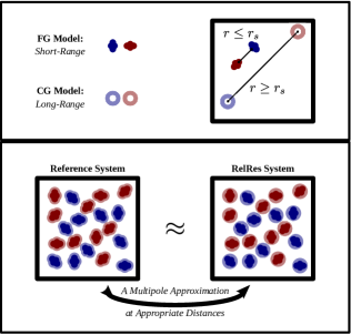
Figure 2: A schematic representation of our multiscale approach for nonpolar systems. The red and blue colors mean that we formally have two different molecules here. The top panel characterizes the geometrical FG and isotropic CG models on its left, and on its right, it illustrates that the former applies between atomistic coordinates, if their relative separation is small, and the latter applies between gravitational centers, if their relative separation is large. The bottom panel basically shows two molecular simulations, for the reference system on the left and for the RelRes system on the right. The arrow represents the MPIL parameterization, which makes the two systems approximately equal to each other.

Let us now cast the interaction between the molecular pair of Fig. 1 as a single function by using Eqs. 39 and 40. For this purpose, we must again remember the MPIL that we thoroughly discussed above. If the molecules of Fig. 1 are near to each other, the approximation of MPIL is unreasonable, and the FG potential of Eq. 39 is the relevant one. If the molecules of Fig. 1 are far from each other, the approximation of MPIL is legitimate, and the CG potential of Eq. 40 is the relevant one. We illustrate these ideas for nonpolar molecules in the top panel of Fig. 2. This is in fact the main idea of RelRes, and we define its potential as follows:

$$\tilde{u}\left(r_{\mu_{i}\nu_{j}};r_{ij}\right)=\sum_{\mu_{i}\nu_{j}}{\displaystyle\tilde{u}_{\mu_{i}\nu_{j}}^{FG}\left(r_{\mu_{i}\nu_{j}}\right)+\tilde{u}_{ij}^{CG}\left(r_{ij}\right)}$$ (41)

In essence, RelRes is a linear combination of $\tilde{u}_{\mu_{i}\nu_{j}}^{FG}$ and $\tilde{u}_{ij}^{CG}$, which are slight modifications of the FG and CG potentials of Eqs. 39 and 40, respectively; we thoroughly discuss these functions below. Besides, note that we emphasize in Eq. 41 that the RelRes potential is a function of various pairwise distances (i.e., atomistic coordinates, $r_{\mu_{i}\nu_{j}}$, and gravitational centers, $r_{ij}$); in such a way, RelRes maintains all degrees of freedom. Note also that the dependence on $\xi_{\mu_{i}\nu_{j}}$ and $\cos\theta_{\mu_{i}\nu_{j}}$ has been omitted here for clarity, especially since these variables do not have any effect on nonpolar molecules.

The modifications of the FG and CG potentials must ensure that for small relative separations, $\tilde{u}_{\mu_{i}\nu_{j}}^{FG}=u_{\mu_{i}\nu_{j}}^{FG}$ while the derivative of $\tilde{u}_{ij}^{CG}$ is zero, and for large relative separations, $\tilde{u}_{\mu_{i}\nu_{j}}^{CG}=u_{\mu_{i}\nu_{j}}^{CG}$ while the derivative of $\tilde{u}_{ij}^{FG}$ is zero. Their exact functionalities are not unique, yet we choose the following piecewise functions for our purposes:

$$\tilde{u}_{\mu_{i}\nu_{j}}^{FG}\left(r\right)=\begin{cases}\begin{array}[]{c}u_{\mu_{i}\nu_{j}}^{FG}\left(r\right)-u_{\mu_{i}\nu_{j}}^{FG}\left(r_{s}\right)\\ 0\end{array}&\begin{array}[]{c}\mathrm{if}\quad r\leq r_{s}\\ \mathrm{if}\quad r\geq r_{s}\end{array}\end{cases}$$ (42)

$$\tilde{u}_{ij}^{CG}\left(r\right)=\begin{cases}\begin{array}[]{c}u_{ij}^{CG}\left(r_{s}\right)\\ u_{ij}^{CG}\left(r\right)\end{array}&\begin{array}[]{c}\mathrm{if}\quad r\leq r_{s}\\ \mathrm{if}\quad r\geq r_{s}\end{array}\end{cases}$$ (43)

The switching distance $r_{s}$ is a constant that represents the relative separation at which the MPIL supposedly switches from being unreasonable to being legitimate. Note that the vertical shifts $u_{\mu_{i}\nu_{j}}^{FG}\left(r_{s}\right)$ and $u_{ij}^{CG}\left(r_{s}\right)$ merely ensure that the corresponding forces are continuous throughout the domains; through the linear combination of RelRes, these vertical shifts approximately cancel each other out, with the extent of the cancellation depending on how many nonzero terms the summation of Eq. 41 includes.

Eq. 41 is actually the pairwise version of RelRes, which only applies for a molecular pair in vacuum. Extending RelRes for a multiscale simulation with many molecules, we define the complete version of RelRes through a summation over all different pairs of molecules in the system:

$$\tilde{U}=\frac{1}{2}\sum_{i\neq j}\tilde{u}\left(r_{\mu_{i}\nu_{j}};r_{ij}\right)$$

$$\tilde{U}=\frac{1}{2}\sum_{i\neq j}\left[\sum_{\mu_{i}\nu_{j}}{\displaystyle\tilde{u}_{\mu_{i}\nu_{j}}^{FG}\left(r_{\mu_{i}\nu_{j}}\right)+\tilde{u}_{ij}^{CG}\left(r_{ij}\right)}\right]$$ (44)

We omit the functionality of this complete version of RelRes throughout our work for clarity. This Hamiltonian introduces a notable conceptual complexity, as compared with Eq. 41 of the pairwise case. For a molecular pair in vacuum, the entire system is basically either a pure FG or CG scenario: If the molecules are near to each other, they are both described by the FG model, and if the molecules are far from each other, they are both described by the CG model (of course, there are subtleties for moderate relative separations). Nevertheless, in the case of a molecular simulation of a realistic liquid, the situation is completely different, with the system being neither purely FG nor CG, but instead having a hybrid nature: Each molecule simultaneously embodies both models, and a given molecule interacts with its near neighbors via the FG potential and with its far neighbors via the CG potential. The bottom panel of Fig. 2 illustrates a RelRes system for a nonpolar scenario, which emphasizes that all molecules embody both molecular resolutions.

Let us also discuss RelRes in terms of its $r_{s}$ parameter, labeling such a dependence as $\tilde{U}_{r_{s}}$. The two limits of $r_{s}$ are of particular importance for emphasis: $\tilde{U}_{\infty}$ is identical with the corresponding Hamiltonian of the pure FG system, and $\tilde{U}_{0}$ is identical with the corresponding Hamiltonian of the pure CG system. The former is the basis for reference mixtures. Such a system has $r_{s}\rightarrow\infty$ (i.e., a system with just FG and no CG interactions), and it is depicted in the bottom panel of Fig. 2. An inherent goal for RelRes with an arbitrary $r_{s}$ is of approximately capturing all behavior of its corresponding reference mixture (e.g., $\tilde{U}_{r_{s}}\approx\tilde{U}_{\infty}$). For completeness, let us also define the entire system Hamiltonian:

$$\tilde{E}=K+U_{0}+\tilde{U}$$ (45)

$K$ is the kinetic energy, while $U_{0}$ accounts for all intramolecular interactions. Note that these do not have a tilde above them. This is because RelRes maintains all degrees of freedom, and in turn, its $K$, as well as its $U_{0}$, is strictly unaltered with the corresponding functions of the reference system (e.g., $K_{r_{s}}=K_{\infty}$).

3 Computational Validation

We now turn our attention for testing the efficacy of our multiscale approach in describing reference systems . We do this via molecular simulations, complementing in turn the initial examination of our previous publication [1]. Our original work was a proof of concept that RelRes is very successful in describing (nonpolar) multi-component and multi-phase systems across state space; by invoking a tuning parameter in our Hamiltonian, we also showed that MPIL is in fact the ideal choice for the potential beyond nearest neighbors. Consequently for simplicity in this current work, we only examine uniform liquids, taking MPIL for granted in all of our systems. Here, we instead focus on systematically varying the distance at which we switch between the FG and CG potentials. Besides, we also complement our initial work by showing that RelRes with MPIL works well not only for static behavior but also for dynamic behavior.

3.1 Constructing the Molecular Simulations

Let us begin by thoroughly discussing the general implementation of our molecular simulations. It is almost identical with the implementation we had in our original publication [1]; we emphasize important aspects which are different. Above all, we again perform our molecular simulations with the GROMACS package, specifically its 4.6 version [44]. If we do not specify here certain features of the molecular simulations, that basically means that the default values are used.

In the current publication, all of our systems contain a total of 2000 (identical) molecules: All of them are dumbbell-like molecules (e.g., ethenes), with two FG sites and one CG site, meaning that $n=2$. All FG atomistic coordinates have mass $m$, and all CG gravitational centers have mass zero; the latter is constructed via equal weights of the former.

In all cases, the LJ potential is the sole component for the interactions between molecules; this in turn sets the length and energy parameters, $\sigma$ and $\epsilon$, respectively, for our work. For a practical implementation of RelRes so that there are no singularities in Newtonian trajectories, we modify the step functionality of Eqs. 42 and 43: In each of these in the interval $\left[r_{s}-\delta r_{s},r_{s}+\delta r_{s}\right]$, we introduce the following four-term polynomial in terms of the inverse distance:

$$f\left(r\right)=\frac{\gamma_{6}}{r^{6}}+\frac{\gamma_{12}}{r^{12}}+\frac{\gamma_{18}}{r^{18}}+\frac{\gamma_{24}}{r^{24}}$$ (46)

The four coefficients $\gamma$ are determined by ensuring that the potential, as well as its derivative, is continuous at its two boundaries, $r_{s}\pm\delta r_{s}$. We vary $r_{s}$ between $1.1\sigma$ and $1.9\sigma$ at intervals of $0.2\sigma$, and we set $\delta r_{s}=0.0625\sigma$. On an analogous note, rather than sharply truncating all potentials at $2.5\sigma$ with a step function, we invoke the sigmoid function above between $2.25\sigma$ and $2.75\sigma$. Note that all interactions in our reference system, denoted by $r_{s}\rightarrow\infty$, practically vanish beyond this distance.

The intramolecular energetics are mostly governed by elastic bonds, which is unlike our previous publication that had all bonds being rigid. Here, the distance of each bond is $0.5\sigma$, while its spring is $2000\epsilon/\sigma^{2}$. Comparing with a conventional bond, our distance is shorter by a significant fraction, while our spring is about an order of magnitude weaker. This is purposefully done as a stringent test: If RelRes can work on our large flexible molecules, it can also work on small stiff molecules.

In all cases, the protocol that we use involves a sequence of molecular simulations at a temperature of $1.0\epsilon/k$, with $k$ being Boltzmann’s constant. The initial molecular simulation is of the reference liquid, and it is distinct in that it is coupled to a barostat, whose pressure is $1.0\epsilon/\sigma^{3}$; the purpose of this molecular simulation is to fix the system size for the entire sequence, while all of its results are disregarded. The rest of the molecular simulations are subsequently in the canonical ensemble: One of them is of the reference liquid, while the rest are RelRes systems of different switching distances. Besides, all molecular simulations evolve via Newtonian equations of motion. Each molecular simulation starts with an equilibration phase of $5,000$ steps of size $0.002\tau$ and ends with a production phase of $1,000,000$ steps of size $0.001\tau$; note that $\tau=\sqrt{m\sigma^{2}/\epsilon}$ is our unit of time. Realize that all molecular simulations that we perform in this work are of single-component and single-phase systems.

3.2 Computing Static and Dynamic Features

Above all, we thoroughly examine in our work several structural correlations, usually in terms of relative separation $r_{ij}$; we frequently omit the $ij$ indices throughout most of our work. For this purpose, we record the positions of all molecules every $100$ steps of the molecular simulation. The domain of our $r$ goes completely from the origin to the edge of the system box; we discretize it by $1000$ bins.

Foremost, we look at radial distributions, $g$, between the midpoints of bonds. For comparison between radial distributions, it is convenient to invoke a functional for them. We particularly choose the Jensen-Shannon entropy:

$$S_{JS}=S\left[\frac{1}{2}\left(g_{r_{s}}+g_{\infty}\right)\right]-\frac{1}{2}\left(S\left[g_{r_{s}}\right]+S\left[g_{\infty}\right]\right)$$ (47)

with the conventional entropy taking on this definition:

$$S\left[g\right]=-\intop\kappa gr^{2}\ln\left(\kappa gr^{2}\right)dr$$ (48)

$\kappa$ is just the normalization constant (i.e., $\intop\kappa gr^{2}=1$), which is inversely proportional with the system volume. In Eq. 47, the term on the left (i.e., $S\left[\frac{1}{2}\left(g_{\infty}+g_{r_{s}}\right)\right]$) is one entropy, altogether for an average of two distributions, and the term on the right (i.e., $\frac{1}{2}\left(S\left[g_{\infty}\right]+S\left[g_{r_{s}}\right]\right)$) is an average of two entropies, each for one distribution. As such, the Jensen-Shannon entropy is a functional of two radial distributions, which just measures the disparity between them: Obviously if $g_{r_{s}}\approx g_{\infty}$, $S_{JS}\approx 0$, and $S_{JS}$ increases as the discrepancy between $g_{r_{s}}$ and $g_{\infty}$ intensifies.

Note that while in the previous work, we presented $g$ between atomistic coordinates, in the current work, we basically focus on $g$ between gravitational centers. In turn, it is important to complement these radial distributions with orientational correlations. By letting a bond be a vector, we define $\vec{s}_{i}$ and $\vec{s}_{j}$ as the respective directions of molecules $i$ and $j$. We particularly focus on computing the moments of their corresponding dot product, $\vec{s}_{i}\cdot\vec{s}_{j}$, as a function of the relative separation between the midpoints of the bonds. Most of our case studies have symmetry in their molecules, and thus for $\vec{s}_{i}\cdot\vec{s}_{j}$, the average vanishes but the variance persists. We consequently present in our work only the latter, $\left\langle\left(\vec{s}_{i}\cdot\vec{s}_{j}\right)^{2}\right\rangle$; note that $\left\langle\left(\vec{s}_{i}\cdot\vec{s}_{j}\right)^{2}\right\rangle=\frac{1}{3}$ for decorrelated cases. Moreover, the bond vectors can be cast as a linear decomposition in terms of two components $\vec{s}_{i}=\vec{s}_{i}^{\|}+\vec{s}_{i}^{\bot}$ and $\vec{s}_{j}=\vec{s}_{j}^{\|}+\vec{s}_{j}^{\bot}$: In terms of the relative separation between molecules $i$ and $j$, $\left\{\vec{s}_{i}^{\|},\vec{s}_{j}^{\|}\right\}$ are the components parallel to $\vec{r}_{ij}$, and $\left\{\vec{s}_{i}^{\bot},\vec{s}_{j}^{\bot}\right\}$ are the components perpendicular to $\vec{r}_{ij}$. In turn, we have the following:

$$\left\langle\left(\vec{s}_{i}\cdot\vec{s}_{j}\right)^{2}\right\rangle=\left\langle\left(s_{i}^{\|}s_{j}^{\|}\right)^{2}\right\rangle+2\left\langle s_{i}^{\|}s_{j}^{\|}s_{i}^{\bot}s_{j}^{\bot}\right\rangle+\left\langle\left(s_{i}^{\bot}s_{j}^{\bot}\right)^{2}\right\rangle$$

$$\left\langle\left(\vec{s}_{i}\cdot\vec{s}_{j}\right)^{2}\right\rangle\approx\left\langle\left(s_{i}^{\|}s_{j}^{\|}\right)^{2}\right\rangle+\left\langle\left(s_{i}^{\bot}s_{j}^{\bot}\right)^{2}\right\rangle$$ (49)

The approximation is introduced here because in most of our case studies, we observe that the cross term in the above expression is rather negligible, and thus, we only present the two main components, $\left\langle\left(s_{i}^{\|}s_{j}^{\|}\right)^{2}\right\rangle$ and $\left\langle\left(s_{i}^{\bot}s_{j}^{\bot}\right)^{2}\right\rangle$, of this orientational function; realize that $\left\langle\left(s_{i}^{\|}s_{j}^{\|}\right)^{2}\right\rangle=\frac{1}{9}$ and $\left\langle\left(s_{i}^{\bot}s_{j}^{\bot}\right)^{2}\right\rangle=\frac{2}{9}$ for an ideal gas.

Besides these static functions, we also examine dynamic functions, something that we did not at all do in our original publication. Specifically, we look at the squared displacement $\left\langle\left(\vec{r}_{t}-\vec{r}_{0}\right)^{2}\right\rangle$, as well as its derivative, $\partial_{t}\left\langle\left(\vec{r}_{t}-\vec{r}_{0}\right)^{2}\right\rangle$. $\vec{r}_{t}$ is the position of molecule $i$ or $j$ at a given time $t$, and the index $0$ is of course for zero time. Besides, we also examine an orientational correlation $\left\langle\vec{s}_{t}\cdot\vec{s}_{0}\right\rangle$. $\vec{s}_{t}$ is analogous with the dumbbell directions introduced earlier; just as with the squared displacement, we have here the time index, while the molecule indices, $i$ or $j$, are omitted for clarity. Importantly in calculating these transport functions, we employ an algorithm of multiple time origins, in fact using each recorded step for such purposes.

We furthermore examine thermal properties in our work. We foremost look at the average $\left\langle\widetilde{U}\right\rangle$ and variance $\left\langle\delta\widetilde{U}^{2}\right\rangle$ of the defining equation of RelRes. For convenience, we normalize both by the corresponding values for the reference liquid: $\left\langle\widetilde{U}\right\rangle_{r_{s}}^{*}=\left\langle\widetilde{U}\right\rangle_{r_{s}}/\left\langle\widetilde{U}\right\rangle_{\infty}$ and $\left\langle\delta\widetilde{U}^{2}\right\rangle_{r_{s}}^{*}=\left\langle\delta\widetilde{U}^{2}\right\rangle_{r_{s}}/\left\langle\delta\widetilde{U}^{2}\right\rangle_{\infty}$; as we frequently do, we omit the index of $r_{s}$ for these thermal properties. Besides, we also look at a transport function of the total energy, $\left\langle\delta\widetilde{E}_{t}\delta\widetilde{E}_{0}\right\rangle/\left\langle\delta\widetilde{E}^{2}\right\rangle$, computing it again using multiple time origins. All of our thermal properties are based on probing our molecular simulations every $10$ steps.

3.3 Examining Elementary Dumbbells

We begin by examining a system of elementary dumbbells. These can be considered as ethenes, and one such molecule is depicted in Fig. 3. Such a dumbbell has two identical FG sites, with $\sigma$ and $\epsilon$ for its LJ parameters. By the MPIL, this means that the respective CG site has $\sigma$ and $4\epsilon$ for its LJ parameters since $n=2$. The inherent bond of these elementary dumbbells is set at at a distance of $0.5\sigma$. The density for this system is $1.00\sigma^{3}/m$.

The radial distribution between the dumbbells is given in the top panel of Fig. 3. This structural correlation for the reference liquid is given here as the solid black curve; the remaining dashed curves are for the RelRes systems, with each color representing a different switching distance. All of these switching distances give a sufficient description of the radial distribution of the reference system, and it is clear that as $r_{s}$ increases, the capability of RelRes improves, in an apparently asymptotic manner: While for $r_{s}=1.3\sigma$ (i.e., the blue curve), the replication is fairly decent, for $r_{s}=1.7\sigma$ (i.e., the red curve), the replication is essentially perfect; in fact, $r_{s}=1.5\sigma$ (i.e., the violet curve) already captures the radial distribution of the reference system as well as one may desire. The systematic observation here is reminiscent with the one we had in the original publication [1]: RelRes captured structural correlations with $r_{s}\approx 1.1\sigma$ equitably yet with $r_{s}\approx 1.6\sigma$ splendidly.

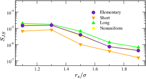
Figure 4: The Jensen-Shannon entropy, $S_{JS}$, for the radial distribution, plotted as a function of the switching distance $r_{s}$ in RelRes. Each curve is for a different system. The indigo color is for the molecules which have identical LJ parameters between their two sites, $\epsilon$ and $\sigma$, and the corresponding bond length is $0.5\sigma$. The orange and green curves refer to the systems with bond lengths of $0.3\sigma$ and $0.7\sigma$, while their LJ parameters are also uniform. The almost hidden yellow curve corresponds with $\left\{1.61\epsilon,0.62\epsilon\right\}$ and $\left\{0.85\sigma,1.18\sigma\right\}$ for its LJ parameters, while its bond is identical with that of the base case. Importantly, note that the entropy is in logarithmic scale. Besides, the lines here just serve as guides.

For the purpose of better clarifying this asymptotic behavior, we invoke the Jensen-Shannon entropy, as defined by Eq. 47. For each of the relevant curves in Fig. 3, we calculate $S_{JS}$, and we plot it (i.e., an indigo circle) in terms of the switching distance in Fig. 4. Clearly, this entropy is monotonic throughout most of the domain of $r_{s}$, and considering the logarithmic scale here, $S_{JS}$ is roughly an exponential decay of the distance; this is especially true around $r_{s}=1.5\sigma$, which we mentioned in the context of Fig. 3 as the critical switching distance for adequately capturing the radial distribution of the reference system. Thus, we confirm here our earlier observation: RelRes improves asymptotically as $r_{s}$ approaches infinity. Importantly, it appears that the asymptote is practically reached at $r_{s}\approx 1.5\sigma$: At this distance, the discrepancy between the radial distributions almost vanishes, and in turn, $S_{JS}$ becomes rather negligible.

So why is $1.5\sigma$ the critical distance for switching between the FG and CG potentials in RelRes? For this purpose, we now look at orientational correlations in the bottom panel of Fig. 3. Let us begin by discussing the black solid curve, which is $\left\langle\left(\vec{s}_{i}\cdot\vec{s}_{j}\right)^{2}\right\rangle$ of the reference liquid. Notice that while it clearly has a maximum and a minimum early on, it quickly flattens out after the ensuing inflection at $1.42\sigma$. This consequently explains why $1.5\sigma$ is an excellent choice for $r_{s}$ in RelRes: At this distance, the dumbbell directions apparently become decorrelated, and the influence of these orientational degrees of freedom becomes negligible on the various structural correlations of the system (e.g., radial distributions). Interestingly, the flattening of $\left\langle\left(\vec{s}_{i}\cdot\vec{s}_{j}\right)^{2}\right\rangle$ in the bottom panel happens just around the middle between the respective maximum and minimum in $g$ of the corresponding top panel (i.e., the relative separation of $1.54\sigma$); this is also around the respective inflection of $g$ (i.e., the relative separation of $1.46\sigma$), which we mark by a vertical brown line in both panels. This means that as soon as nearest neighbors depart from each other, their directions quickly become decorrelated.

Let us continue examining the two main components of $\left\langle\left(\vec{s}_{i}\cdot\vec{s}_{j}\right)^{2}\right\rangle$, as given in Eq. 49. For the reference system, these are plotted as gray curves in the bottom panel of Fig. 3, the lower one is for $\left\langle\left(s_{i}^{\|}s_{j}^{\|}\right)^{2}\right\rangle$ and the higher one is for $\left\langle\left(s_{i}^{\bot}s_{j}^{\bot}\right)^{2}\right\rangle$; importantly, realize that their summation essentially yields the black curve. Surprisingly, the behavior of $\left\langle\left(\vec{s}_{i}\cdot\vec{s}_{j}\right)^{2}\right\rangle$ is very distinct from its components: While $\left\langle\left(\vec{s}_{i}\cdot\vec{s}_{j}\right)^{2}\right\rangle$ becomes mostly decorrelated as the molecules leave the primary coordination shell, its components are still correlated even as the molecules enter the secondary coordination shell. In fact, $\left\langle\left(s_{i}^{\|}s_{j}^{\|}\right)^{2}\right\rangle$ and $\left\langle\left(s_{i}^{\bot}s_{j}^{\bot}\right)^{2}\right\rangle$ appear as mirror images of each other, especially beyond $r\approx 1.5\sigma$, with the fluctuations between the maxima and minima of the two curves occurring at the same locations. In turn, once we sum these two functions, the extrema cancel each other, yielding the overall function which is basically flat beyond $r\approx 1.5\sigma$. The locations of the initial maximum of $\left\langle\left(s_{i}^{\|}s_{j}^{\|}\right)^{2}\right\rangle$ and the initial minimum of $\left\langle\left(s_{i}^{\bot}s_{j}^{\bot}\right)^{2}\right\rangle$ occur at $1.49\sigma$ and $1.54\sigma$, which is again almost identical with the ideal $r_{s}$ of $1.5\sigma$.

Finally, let us not forget the dotted curves in the bottom panel of Fig. 3. Their coloring is equivalent with that of the corresponding top panel, with each color representing a different $r_{s}$ in RelRes; besides, the function to which each dotted curve pertains corresponds with the function of its neighboring solid curve. Importantly, RelRes captures the orientational correlation with its components perfectly well, regardless of which switching distances we use. This is in contrast with the radial distribution, which is noticeably influenced by $r_{s}$.

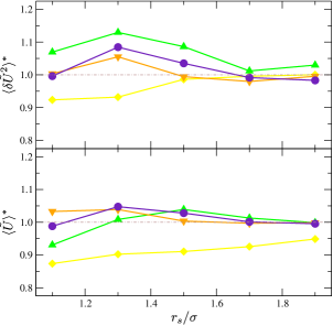
Figure 5: Energetic functionals plotted as a function of the switching distance $r_{s}$ in RelRes. Particularly, the average $\left\langle\widetilde{U}\right\rangle$ and variance $\left\langle\delta\widetilde{U}^{2}\right\rangle$ of the configurational energy is given in the bottom and top panels respectively; the asterisk denotes that these functionals are normalized by the respective value of the reference system. Besides, the color coding here is identical with that of Fig. 4.

We now move on to examine thermal properties of these elementary dumbbells. We specifically look at functionals of the configurational Hamiltonian of RelRes, presenting, as a function $r_{s}$, its normalized average $\left\langle\widetilde{U}\right\rangle$ and variance $\left\langle\delta\widetilde{U}^{2}\right\rangle$ in the bottom and top panels of Fig. 5, respectively. The coloring here is analogous with Fig. 4. Focus again on the indigo circles: Because of normalization, they fluctuate about the horizontal brown line which is of course set at unity. In fact, for all switching distances, the average and variance are essentially both within a fraction of $0.05$ from their reference values. Importantly, we notice that a dampening effect of the fluctuation, with both the average and variance eventually reaching unity. Besides, the fluctuating characteristic of the symbols in this figure is in striking contrast to the observation we made for the functional of the structural correlations in Fig. 4, which showed an asymptotic behavior with $r_{s}$. Bearing also in mind Fig. 3, this means that if one is fine with a decent yet rough description of radial distributions in a liquid, one can still adequately capture thermal properties, together with orientational correlations, while using just a modest switching distance in RelRes that does not entirely account for all nearest neighbors. Finally, these systematic findings are analogous with the observations we made in our previous work for the pressure, together with its corresponding response function. For both of our switching distances there, $r_{s}\approx 1.1\sigma$ and $r_{s}\approx 1.6\sigma$, RelRes was very successful once we used it together with MPIL; [1]. In general, the excellent replication of thermal properties reiterates the validity of the MPIL approximation, which is essentially based on energy conservation.

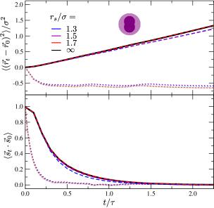
Figure 6: Dynamic correlations for the elementary dumbbell scenario. Much of the coding here is equivalent with Fig. 3, but all of the current functions are different from the elementary case. Everything is plotted in terms of time $t$. The top panel plots the squared displacement $\left\langle\left(\vec{r}_{t}-\vec{r}_{0}\right)^{2}\right\rangle$ of a given molecule as the black curve for the reference system, together with its neighboring dashed lines for the RelRes systems; the corresponding negative derivative of this function $-\partial_{t}\left\langle\left(\vec{r}_{t}-\vec{r}_{0}\right)^{2}\right\rangle$ is given as the gray curve, together with its dotted lines. In an analogous manner, the bottom panel plots the orientational function $\left\langle\vec{s}_{t}\cdot\vec{s}_{0}\right\rangle$ as the black curve, together with its neighboring dashed lines; the gray curve, together with its dotted lines, represents the energetic function $\left\langle\delta\widetilde{E}_{t}\delta\widetilde{E}_{0}\right\rangle/\left\langle\delta\widetilde{E}^{2}\right\rangle$.

So far, considering our original publication as well, we have only examined static behavior; we now turn our attention to dynamic behavior. We consequently plot various transport functions in terms of time, $t$, in Fig. 6. The coloring here is again analogous with Fig. 3: While all solid curves are for the reference liquid, the dashed and dotted lines are for the RelRes systems with varying $r_{s}$. In the top panel for the reference liquid, we give $\left\langle\left(\vec{r}_{t}-\vec{r}_{0}\right)^{2}\right\rangle$ as the black line, with its negative derivative $-\partial_{t}\left\langle\left(\vec{r}_{t}-\vec{r}_{0}\right)^{2}\right\rangle$ as the gray one. In the bottom panel for the reference liquid, the orientational correlation $\left\langle\vec{s}_{t}\cdot\vec{s}_{0}\right\rangle$ is given as the black line. Besides these structural functions, we also present here a thermal function, particularly for the total energy, $\left\langle\delta\widetilde{E}_{t}\delta\widetilde{E}_{0}\right\rangle/\left\langle\delta\widetilde{E}^{2}\right\rangle$, as the gray line. Of course, the functionality of the colored lines is the same as that of their respective neighboring curves.

In an all cases, irrespective of the value of $r_{s}$, RelRes satisfactorily captures the transport functions of the reference system. Of course, there are some nuances between the various transport functions in terms of $r_{s}$, and these dynamic characteristics are reminiscent of our observations for the static features. For example, $r_{s}=1.7\sigma$ is required for a flawless replication of the translational $\left\langle\left(\vec{r}_{t}-\vec{r}_{0}\right)^{2}\right\rangle$, yet for the orientational $\left\langle\vec{s}_{t}\cdot\vec{s}_{0}\right\rangle$, only $r_{s}=1.3\sigma$ can not excellently capture the behavior of the reference liquid. Besides, for the thermal function $\left\langle\delta\widetilde{E}_{t}\delta\widetilde{E}_{0}\right\rangle/\left\langle\delta\widetilde{E}^{2}\right\rangle$, all switching distances yield a perfect description of this transport function. In summary, in terms of $r_{s}$, we notice the same trends for dynamic behavior as we do with static behavior: Thermal properties can be superbly captured even with a surprisingly small $r_{s}$, but structural correlations require a relatively large $r_{s}$; for the latter, we notice that its orientational correlations are rather feasible of capturing as compared with their translational counterparts. Specifically for these elementary dumbbells, it appears that $r_{s}=1.5\sigma$ can capture the entire behavior of the reference liquid very well, and thus, this is our recommended switching distance for these molecules. This in turn reiterates one of our main findings of the original publication: RelRes works best if molecules interact with each via a FG potential between nearest neighbors and a CG potential between other neighbors.

3.4 Varying the Bond Length

We continue by examining dumbbells in which we vary the length of the bonds. In particular, we construct two systems, one with short dumbbells (i.e., $\ell=0.3\sigma$) and one with long dumbbells (i.e., $\ell=0.7\sigma$); representative sketches are given in Figs. 7 and 8, respectively. The modification of the bond length does not alter the LJ parameters of the FG and CG sites: They are again $\sigma$ and $\epsilon$ for the former, and $\sigma$ and $4\epsilon$ for the latter. The system density is $1.34$ for the short molecules and $0.78$ for the long molecules, in units of $m/\sigma^{3}$.

The structural correlations for the short and long dumbbells are given in Figs. 7 and 8, respectively, which are basically analogous with those of Fig. 3. All orientational functions of the reference liquids are perfectly captured by RelRes, regardless of the switching distance that we use; we consequently give in the respective bottom panels the $r_{s}=1.5\sigma$ curve. Conversely, the radial distributions are given in the respective top panels; notice importantly the cyan curve (i.e., $r_{s}=1.1\sigma$) for the $\ell=0.3\sigma$ case and the magenta curve (i.e., $r_{s}=1.9\sigma$) for the $\ell=0.7\sigma$. In essence for each case, we have shifted our systematic $r_{s}$ examination by $0.2\sigma$. This is because we observe that RelRes captures the radial distributions at a switching distance that differs by roughly $0.2\sigma$ as compared with the $\ell=0.5\sigma$ of Fig. 3: The apparently asymptotic $r_{s}$ is $1.3\sigma$ in Fig. 7 and $1.7\sigma$ in Fig. 8. It is of course natural that the ideal $r_{s}$ for the short dumbbells is less than the ideal $r_{s}$ for the long dumbbells, since the former are more “sphere-like” than the latter. This further means that RelRes works better as the molecular size decreases. As a further analysis, we compute $S_{JS}$ for these radial distributions, plotting them in Fig. 4 as orange (downward) triangles for $\ell=0.3\sigma$ and as green (upward) triangles for $\ell=0.7\sigma$. For these two cases, we again observe an essentially exponential decay. We also reaffirm that the efficacy of RelRes is more deficient for the long molecules than for the short molecules, considering that $S_{JS}$ for $\ell=0.3\sigma$ is less than that for $\ell=0.7\sigma$ by about an order of magnitude; remember that $S_{JS}\rightarrow 0$ means that we are approaching perfect replication of the radial distribution.

In the context of Fig. 3 for $\ell=0.5\sigma$, we have thoroughly discussed that the recommended value of $r_{s}$ is signaled by structural correlations. We find that this is still the case here once we vary the bond length of the dumbbells. Most importantly, in the bottom panels of Figs. 7 and 8, we again notice the flattening of $\left\langle\left(\vec{s}_{i}\cdot\vec{s}_{j}\right)^{2}\right\rangle$ beyond a certain distance, which stems in the mirroring behavior of the maxima and minima of its components $\left\langle\left(s_{i}^{\|}s_{j}^{\|}\right)^{2}\right\rangle$ and $\left\langle\left(s_{i}^{\bot}s_{j}^{\bot}\right)^{2}\right\rangle$ that cancel each other. We summarize all the critical distances associated with these orientational correlations, as well as with the translational ones in the respective top panels, in Tab. 1. Among these different bond lengths, we generally notice the same trends: The inflection in $\left\langle\left(\vec{s}_{i}\cdot\vec{s}_{j}\right)^{2}\right\rangle$ comes just before the inflection in $g$, and this is followed consecutively by the the minimum in $\left\langle\left(s_{i}^{\bot}s_{j}^{\bot}\right)^{2}\right\rangle$ and the maximum in $\left\langle\left(s_{i}^{\|}s_{j}^{\|}\right)^{2}\right\rangle$, with the midpoint between the extrema in $g$ being around there as well. For a given bond length, the most important aspect of these distances is that they almost all occur within $0.1\sigma$ of each other, and they are roughly the same as the estimate for the asymptotic $r_{s}$ via our systematic RelRes examination.

As such, it appears that if one is interested in determining the ideal switching distance, there may be no need of constructing many RelRes systems with different $r_{s}$: One can just look at the structural correlations of the reference liquid, with the radial distribution being perhaps the most feasible choice. As such, we consequently again draw vertical lines in Figs. 7 and 8 that represent their inflections in $g$. Nevertheless, we can even go further: For such dumbbells of an arbitrary bond length, we may not even need to do any molecular simulations of the reference liquid at all for determining $r_{s}$ , since it is quite obvious here that the following linear approximation holds:

$$r_{s}\approx\sigma+\ell$$ (50)

This further suggests that for an arbitrary system, one may be able to do a rough estimate for the ideal $r_{s}$ in RelRes just by considering the size of the respective molecules.

Finally, we also calculate thermal properties for these two systems. Analogous with the elementary dumbbells, we plot their average $\left\langle\widetilde{U}\right\rangle$ and variance $\left\langle\delta\widetilde{U}^{2}\right\rangle$ in the bottom and top panels, respectively, of Fig. 5, with the orange (downward) triangles for $\ell=0.3\sigma$ and the green (upward) triangles for $\ell=0.7\sigma$. We again notice the fluctuating trend in all sets here. Importantly, notice that the magnitude of these fluctuations decreases with bond length. This reiterates the fact the RelRes works better for “sphere-like” molecules.

3.5 Examining Nonuniform Dumbbells

We now construct another system, whose molecules again have a bond length of $0.5\sigma$ . In this case however, we are dealing with nonuniform dumbbells in terms of their LJ parameters, although they do still have equal mass across their sites; a sketch of such a molecule is given in Fig. 9. Elaborating on this nonuniformity, one FG site is small yet strong, and one FG site is large yet weak: Their respective length parameters are $6/\left(1+\sqrt{37}\right)\approx 0.85$ and $\left(1+\sqrt{37}\right)/6\approx 1.18$, in units of $\sigma$, and their respective energy parameters are $\left(1+\sqrt{5}\right)/2\approx 1.61$ and $2/\left(1+\sqrt{5}\right)\approx 0.62$, in units of $\epsilon$; notice that the mixed interaction between these two still has the standard $\sigma$ and $\epsilon$ parameters. Using MPIL, we obtain that the ideal CG site has LJ parameters that are roughly $1.08\sigma$ and $2.76\epsilon$. Importantly, realize that even though these dumbbells are nonuniform, the system itself is still uniform, being a single-component and single-phase liquid. Besides, the density for this system is $0.88\sigma^{3}/m$.

For this dumbbell system, we again perform a systematic examination for the switching distance. We present the corresponding structural correlations in Fig. 9, whose format is identical with that of Fig. 3. We again notice the same trends that we have observed for our elementary dumbbells. For the orientational functions of the bottom panel, the replication is perfect irrespective of the value of $r_{s}$, just as we found in all of our other scenarios. Most importantly, for the radial distributions in the top panel, we find that the asymptotic $r_{s}$ is at $1.5\sigma$, just as we have for our elementary dumbbells (i.e., $\ell=0.5\sigma$). Once we determine all the critical distances in $g$, as well as in $\left\langle\left(\vec{s}_{i}\cdot\vec{s}_{j}\right)^{2}\right\rangle$ with its components, we again find that they are all roughly the same as the ideal $r_{s}$ for RelRes; these are summarized in Tab. 1. Realize now that Eq. 50 still applies for this case, even though we established it while only considering uniform dumbbells. Finally, once we invoke our functionals for the radial distributions, we show in Fig. 4 that for all $r_{s}$, $S_{JS}$ for this nonuniform scenario (i.e., the almost hidden yellow diamonds) is basically identical with its uniform counterpart (i.e., the indigo circles).

All of these observations for the structural correlations of the nonuniform dumbbells, particularly the fact that their relationship with the switching distance of RelRes is identical with that of our elementary dumbbells (i.e., those with the same bond length of $0.5\sigma$, yet which are uniform across their sites), has significant ramifications. For an arbitrary molecule which has much uniformity within it, we do not need to perform any molecular simulations for it for determining its ideal $r_{s}$; all one must do is to construct a system of similar molecules that are actually uniform across their sites (perhaps using the overall mean values for $\sigma$ and $\epsilon$ of the nonuniform molecule). According to our observations, these uniform molecules, whose structural correlations are fairly feasible for computation, would roughly have the same $r_{s}$ as the nonuniform molecules. This fact becomes especially useful once we are dealing with a set of molecules that roughly have the same topology, yet whose sites notably vary in their LJ parameters: If the molecules do not have the linear estimate for $r_{s}$ as given in Eq. 50, we suggest that all one does is measure, via a single molecular simulation, the radial distribution of the reference liquid of the uniform version of these molecules, and we recommend using its inflection in $g$ as the switching distance in RelRes for the entire family of molecules.

We now proceed with the thermal properties of the nonuniform scenario in Fig. 5, which is presented as yellow diamonds. In this case, we actually do not observe the fluctuating trend which we have for all other dumbbell scenario, and instead we have a slight asymptotic behavior; of course, it is very modest as compared with the entropic functionals of Fig. 4. Still, this is not necessarily a drawback for RelRes: If we look at our recommended $r_{s}$ of $1.5\sigma$, the variance in the top panel is off by a negligible fraction, yet the average of the bottom panel is off by a $\sim 0.1$ fraction. Of course, the latter is still satisfactory, especially if one is not too interested in exact values of thermal properties. The discrepancy between the ability of RelRes in retrieving the average and variance may stem in the fact that the latter are related with response functions, and it is well known that these can be perfectly captured if the structural correlations are also perfectly captured, which is our case in this scenario. In fact, the main message here is that while structural correlations of nonuniform molecules can be as feasible of retrieving as those of uniform molecules, nonuniform energetics involve much intricacies with them, and thus a perfect replication is rather difficult to achieve.

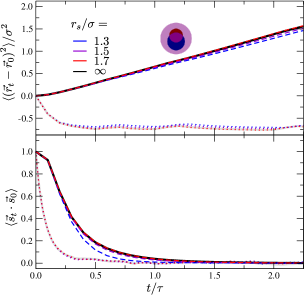
Figure 10: Dynamic correlations for the nonuniform dumbbells, the ones with different LJ parameters across their two sites, $\left\{0.85\sigma,1.18\sigma\right\}$ and $\left\{1.61\epsilon,0.62\epsilon\right\}$. Everything here is essentially equivalent with Fig. 6.

Finally, we examine the transport functions of this nonuniform scenarios; we present them in Fig. 10, which is identical in format with Fig. 6. We again reaffirm our earlier observations. Foremost, RelRes perfectly captures the time behavior of the thermal property of the reference system, regardless of the switching distance. While the transport functions of the structural correlations are also adequately retrieved, there are some subtleties: For perfect replication, $\left\langle\left(\vec{r}_{t}-\vec{r}_{0}\right)^{2}\right\rangle$ of the top panel requires a relatively large $r_{s}$, yet $\left\langle\vec{s}_{t}\cdot\vec{s}_{0}\right\rangle$ of the bottom panel requires a relatively small $r_{s}$. In summary, just as RelRes is successful in capturing static behavior, it is also successful in capturing dynamic behavior, and we basically observe the same capability in describing the nonuniform dumbbells, as with their uniform counterparts.

4 Conclusion

In this current work, we continue our initial effort [1], presenting in turn a comprehensive picture of RelRes with MPIL. As shown in our original communication [1], our hybrid formalism can be thought of as an extension of the common approach in statistical mechanics which describes all interactions beyond a certain distance via a mean field [40, 41, 42, 43]. The main aspect of RelRes is that molecular resolution switches in terms of relative separation: Each molecule embodies both FG and CG models, and a given molecule then interacts with near neighbors via its FG potential and with far neighbors via its CG potential. Via energy conservation, we relate the FG and CG potentials by an arithmetic parameterization, which we call MPIL.

In our current publication, we specifically cast MPIL as a multipole approximation. Reminiscent of the familiar scenario, we do this derivation by assuming that the potential can be cast as a linear combination of inverse powers for the relative separation, and we then perform the common Taylor expansion. We call the leading nonzero term the MPIL, and we show that it naturally fits with RelRes. Note that in our original publication, we naively assumed infinite separation, in turn readily attaining MPIL [1]; this current work is in fact the comprehensive derivation, in which we specifically present the first and second terms of the Taylor series. In our original publication, we already showed that RelRes with MPIL works incredibly well for nonpolar molecules, as complex as a generic tetrachloromethane-thiophene fluid mixture which contains a vacuum cavity [1]. In the current work, we take a better examination at the role of the switching distance, finding an ideal value for it, which can be usually obtained by running a single molecular simulation of the reference mixture. Besides, we also show that RelRes can describe not only statics but also dynamics.

You may notice that RelRes with MPIL bears much resemblance with the famous “cell-multipole” formalism, the algorithm which is frequently mentioned as one of the most computationally powerful methods [45]. For an arbitrary potential of an inverse power, the “cell-multipole” approach also invokes a multipole approximation at appropriate distances: Inside a “cell” at small separations, one evaluates interactions between discrete sites, and outside a “cell” at large separations, one evaluates interactions between continuum patches. A crucial distinction with our multiscale scheme is that the “cell-multipole” strategy considers interaction sites that move freely of each other, in turn lumping them together in arbitrary “cells” in space. In molecular simulations, interaction sites do not move freely of each other as they are constrained by bonds; RelRes, as well as many other multiscale methods [32, 33, 34, 35], uses this signature of molecules, invoking a natural mapping from the FG model to the CG model (i.e., from atomistic coordinates to gravitational centers, respectively). As such, one can think of RelRes with MPIL as an natural modification of the “cell-multipole” approach for molecular simulations. This can be extremely useful, since, despite the fact that the “cell-multipole” method is frequently used in a myriad of systems (e.g., galaxies), it is rarely employed in molecular systems.

As a next step, we are interested in implementing RelRes for polar molecules, specifically for water. Importantly, all the necessary mathematical ingredients have been already derived here. Unlike the nonpolar case, our model for water will have an orientational component, as manifested by its dipole. As we move to biology, we also expect to model various “chains”. Of course, RelRes is only one route for enhancing the efficiency of molecular simulations, and we recommend that one employs it concurrently with other computational approaches for optimal results. For biological systems (e.g., a protein in water), we expect that combining RelRes with explicit-implicit strategies may be especially powerful: Reminiscent of Adaptive Resolution [46], these algorithms switch from an explicit solute near to the origin to an implicit solvent far from the origin [47]; the former is the one that is ideal for being modeled by RelRes. In summary, we emphasize that RelRes with MPIL can be of much use in aiding the study of soft matter via molecular simulations.

Appendix

For proceeding beyond the monopole-monopole term of Eq. 30, we must define several dimensionless variables, reminiscent of Eqs. 3 and 4. Here they are:

$$\overrightarrow{\xi}_{\upsilon_{l}}=\frac{\overrightarrow{\Delta}_{\upsilon_{l}}}{r}$$ (51)

$$\cos\theta_{\upsilon_{l}}=\frac{\overrightarrow{r}\cdot\overrightarrow{\Delta}_{\upsilon_{l}}}{r\Delta_{\upsilon_{l}}}$$ (52)

For compactness in the Appendix, we mostly use here the index $\upsilon$, together with the index $l$: The Latin index corresponds with either $i$ or $j$, and the Greek index corresponds with either $\mu$ or $\nu$. Besides, we also frequently omit yet imply the combination of the $ij$ indices (e.g., $\overrightarrow{r}=\overrightarrow{r}_{ij}$). Using these, together with Eqs. 3 and 4, we derive useful expressions for the dimensionless variables involved in the energy function of Eq. 10:

$$\cos\theta_{\mu_{i}\nu_{j}}\xi_{\mu_{i}\nu_{j}}=\cos\theta_{\nu_{j}}\xi_{\nu_{j}}-\cos\theta_{\mu_{i}}\xi_{\mu_{i}}$$ (53)

$$\xi_{\mu_{i}\nu_{j}}^{2}=\xi_{\nu_{j}}^{2}-2\left(\overrightarrow{\xi}_{\nu_{j}}\cdot\overrightarrow{\xi}_{\mu_{i}}\right)+\xi_{\nu_{j}}^{2}$$ (54)

Note that we also used here the definition of $\overrightarrow{\Delta}_{\mu_{i}\nu_{j}}$ of Eq. 2.

Let us now proceed by invoking these variables in $c_{ij,\aleph}$. For $\aleph=1$, we specifically substitute Eq. 53 in Eq. 21, attaining the following,

$$c_{ij,1}\left(\xi_{\mu_{i}\nu_{j}},\cos\theta_{\mu_{i}\nu_{j}}\right)=m\sum_{\mu_{i}\nu_{j}}\left[c_{\mu_{i}\nu_{j}}\cos\theta_{\nu_{j}}\xi_{\nu_{j}}\right]-m\sum_{\mu_{i}\nu_{j}}\left[c_{\mu_{i}\nu_{j}}\cos\theta_{\mu_{i}}\xi_{\mu_{i}}\right]$$ (55)

and by invoking the product assumption of Eq. 26, we derive this:

$$c_{ij,1}=m\left(\sum_{\mu_{i}}\mathfrak{c}_{\mu_{i}}\right)\left(\sum_{\nu_{j}}\left[\mathfrak{c}_{\nu_{j}}\cos\theta_{\nu_{j}}\xi_{\nu_{j}}\right]\right)-m\left(\sum_{\nu_{j}}\mathfrak{c}_{\nu_{j}}\right)\left(\sum_{\mu_{i}}\left[\mathfrak{c}_{\mu_{i}}\cos\theta_{\mu_{i}}\xi_{\mu_{i}}\right]\right)$$ (56)

For facilitating the ensuing mathematics, we introduce now $c_{ij,2\mathfrak{p}^{\pm}}$ and $c_{ij,2\mathfrak{q}^{\pm}}$, whose summation yields $c_{ij,2^{\pm}}$:

$$c_{ij,2^{\pm}}=c_{ij,2\mathfrak{p}^{\pm}}+c_{ij,2\mathfrak{q}^{\pm}}$$ (57)

For $\aleph=2^{+}$, we specifically substitute Eq. 53 in Eq. 23, attaining the following,

$$c_{ij,2\mathfrak{p}^{+}}\left(\xi_{\mu_{i}\nu_{j}},\cos\theta_{\mu_{i}\nu_{j}}\right)=-m\sum_{\mu_{i}\nu_{j}}\left[c_{\mu_{i}\nu_{j}}\cos\theta_{\nu_{j}}\xi_{\nu_{j}}\cos\theta_{\mu_{i}}\xi_{\mu_{i}}\right]$$ (58)

$$c_{ij,2\mathfrak{q}^{+}}\left(\xi_{\mu_{i}\nu_{j}},\cos\theta_{\mu_{i}\nu_{j}}\right)=\frac{m}{2}\sum_{\mu_{i}\nu_{j}}\left[c_{\mu_{i}\nu_{j}}\cos^{2}\theta_{\nu_{j}}\xi_{\nu_{j}}^{2}\right]+\frac{m}{2}\sum_{\mu_{i}\nu_{j}}\left[c_{\mu_{i}\nu_{j}}\cos^{2}\theta_{\mu_{i}}\xi_{\mu_{i}}^{2}\right]$$ (59)

and by invoking the product assumption of Eq. 26, we derive this:

$$c_{ij,2\mathfrak{p}^{+}}=-m\left(\sum_{\nu_{j}}\left[\mathfrak{c}_{\nu_{j}}\cos\theta_{\nu_{j}}\xi_{\nu_{j}}\right]\right)\left(\sum_{\mu_{i}}\left[\mathfrak{c}_{\mu_{i}}\cos\theta_{\mu_{i}}\xi_{\mu_{i}}\right]\right)$$ (60)

$$c_{ij,2\mathfrak{q}^{+}}=\frac{m}{2}\left(\sum_{\mu_{i}}\mathfrak{c}_{\mu_{i}}\right)\left(\sum_{\nu_{j}}\left[\mathfrak{c}_{\nu_{j}}\cos^{2}\theta_{\nu_{j}}\xi_{\nu_{j}}^{2}\right]\right)+\frac{m}{2}\left(\sum_{\nu_{j}}\mathfrak{c}_{\nu_{j}}\right)\left(\sum_{\mu_{i}}\left[\mathfrak{c}_{\mu_{i}}\cos^{2}\theta_{\mu_{i}}\xi_{\mu_{i}}^{2}\right]\right)$$ (61)

For $\aleph=2^{-}$, we specifically substitute Eq. 54 in Eq. 24, attaining the following,

$$c_{ij,2\mathfrak{p}^{-}}\left(\xi_{\mu_{i}\nu_{j}},\cos\theta_{\mu_{i}\nu_{j}}\right)=-m\sum_{\mu_{i}\nu_{j}}\left[c_{\mu_{i}\nu_{j}}\left(\overrightarrow{\xi}_{\nu_{j}}\cdot\overrightarrow{\xi}_{\mu_{i}}\right)\right]$$ (62)

$$c_{ij,2\mathfrak{q}^{-}}\left(\xi_{\mu_{i}\nu_{j}},\cos\theta_{\mu_{i}\nu_{j}}\right)=\frac{m}{2}\sum_{\mu_{i}\nu_{j}}\left[c_{\mu_{i}\nu_{j}}\xi_{\nu_{j}}^{2}\right]+\frac{m}{2}\sum_{\mu_{i}\nu_{j}}\left[c_{\mu_{i}\nu_{j}}\xi_{\mu_{i}}^{2}\right]$$ (63)

and by invoking the product assumption of Eq. 26, we derive this:

$$c_{ij,2\mathfrak{p}^{-}}=-m\left(\left(\sum_{\nu_{j}}\left[\mathfrak{c}_{\nu_{j}}\overrightarrow{\xi}_{\nu_{j}}\right]\right)\cdot\left(\sum_{\mu_{i}}\left[\mathfrak{c}_{\mu_{i}}\overrightarrow{\xi}_{\mu_{i}}\right]\right)\right)$$ (64)

$$c_{ij,2\mathfrak{q}^{-}}=\frac{m}{2}\left(\sum_{\mu_{i}}\mathfrak{c}_{\mu_{i}}\right)\left(\sum_{\nu_{j}}\left[\mathfrak{c}_{\nu_{j}}\xi_{\nu_{j}}^{2}\right]\right)+\frac{m}{2}\left(\sum_{\nu_{j}}\mathfrak{c}_{\nu_{j}}\right)\left(\sum_{\mu_{i}}\left[\mathfrak{c}_{\mu_{i}}\xi_{\mu_{i}}^{2}\right]\right)$$ (65)

While the monopoles of Eq. 29 can be readily substituted in most of the above expressions, further manipulation must be performed for employing here the dipoles, as well as the quadrupoles.

As such, let us evaluate some of the summations which appear above, by invoking the dimensionless variables of Eqs. 51 and 52. Here are summations which can be conveniently cast in terms of the dipoles of Eq. 31,

$$\sum_{\upsilon_{l}}\left[\mathfrak{c}_{\upsilon_{l}}\cos\theta_{\upsilon_{l}}\xi_{\upsilon_{l}}\right]=\frac{1}{r^{2}}\sum_{\upsilon_{l}}\left[\mathfrak{c}_{\upsilon_{l}}\left(\overrightarrow{r}\cdot\overrightarrow{\Delta}_{\upsilon_{l}}\right)\right]=\frac{1}{r^{2}}\left(\overrightarrow{r}\cdot\left(\sum_{\upsilon_{l}}\left[\mathfrak{c}_{\upsilon_{l}}\overrightarrow{\Delta}_{\upsilon_{l}}\right]\right)\right)=\frac{1}{r}\left(\hat{r}\cdot\mathfrak{\overrightarrow{p}}_{l,1}\right)$$ (66)

$$\sum_{\upsilon_{l}}\left[\mathfrak{c}_{\upsilon_{l}}\overrightarrow{\xi}_{\upsilon_{l}}\right]=\frac{1}{r}\sum_{\upsilon_{l}}\left[\mathfrak{c}_{\upsilon_{l}}\overrightarrow{\Delta}_{\upsilon_{l}}\right]=\frac{1}{r}\mathfrak{\overrightarrow{p}}_{l,1}$$ (67)

while here are summations which can be conveniently cast in terms of the quadrupoles of Eqs. 32 and 33;

$$\sum_{\upsilon_{l}}\left[\mathfrak{c}_{\upsilon_{l}}\cos^{2}\theta_{\upsilon_{l}}\xi_{\upsilon_{l}}^{2}\right]=\frac{1}{r^{4}}\sum_{\upsilon_{l}}\left[\mathfrak{c}_{\upsilon_{l}}\left(\overrightarrow{r}\cdot\overrightarrow{\Delta}_{\upsilon_{l}}\right)^{2}\right]=\frac{1}{r^{4}}\left(\overrightarrow{r}\overrightarrow{r}:\left(\sum_{\upsilon_{l}}\left[\mathfrak{c}_{\upsilon_{l}}\overrightarrow{\Delta}_{\upsilon_{l}}\overrightarrow{\Delta}_{\upsilon_{l}}\right]\right)\right)=\frac{1}{r^{2}}\left(\hat{\hat{r}}:\mathfrak{\overrightarrow{\overrightarrow{q}}}_{l,2}\right)$$ (68)

$$\sum_{\upsilon_{l}}\left[\mathfrak{c}_{\upsilon_{l}}\xi_{\upsilon_{l}}^{2}\right]=\frac{1}{r^{2}}\sum_{\upsilon_{l}}\left[\mathfrak{c}_{\upsilon_{l}}\Delta_{\upsilon_{l}}^{2}\right]=\frac{1}{r^{2}}\mathfrak{q}_{l,0}$$ (69)

note that we used here a common tensor identity: $\left(\overrightarrow{r}\cdot\overrightarrow{\Delta}_{\upsilon_{l}}\right)^{2}=\left(\overrightarrow{r}\overrightarrow{r}:\overrightarrow{\Delta}_{\upsilon_{l}}\overrightarrow{\Delta}_{\upsilon_{l}}\right)$.

By employing these, together with Eq. 29, we can evaluate the relevant $c_{ij,\aleph}$. For $\aleph=1$, substituting Eq. 66 in Eq. 56, we obtain the following:

$$c_{ij,1}=\frac{m}{r}\mathfrak{c}_{i,0}\left(\hat{r}\cdot\mathfrak{\overrightarrow{p}}_{j,1}\right)-\frac{m}{r}\mathfrak{c}_{j,0}\left(\hat{r}\cdot\mathfrak{\overrightarrow{p}}_{i,1}\right)$$ (70)

This is compactly presented in the main text as Eq. 34. For $\aleph=2^{+}$, substituting Eqs. 66 and 68 in Eqs. 60 and 61, respectively, we obtain the following:

$$c_{ij,2\mathfrak{p}^{+}}=-\frac{m}{r^{2}}\left(\hat{r}\cdot\mathfrak{\overrightarrow{p}}_{j,1}\right)\left(\hat{r}\cdot\mathfrak{\overrightarrow{p}}_{i,1}\right)$$ (71)

$$c_{ij,2\mathfrak{q}^{+}}=\frac{m}{2r^{2}}\mathfrak{c}_{i,0}\left(\hat{\hat{r}}:\mathfrak{\overrightarrow{\overrightarrow{q}}}_{j,2}\right)+\frac{m}{2r^{2}}\mathfrak{c}_{j,0}\left(\hat{\hat{r}}:\mathfrak{\overrightarrow{\overrightarrow{q}}}_{i,2}\right)$$ (72)

For $\aleph=2^{-}$, substituting Eqs. 67 and 69 in Eqs. 64 and 65, respectively, we obtain the following:

$$c_{ij,2\mathfrak{p}^{-}}=-\frac{m}{r^{2}}\left(\mathfrak{\overrightarrow{p}}_{j,1}\cdot\mathfrak{\overrightarrow{p}}_{i,1}\right)$$ (73)

$$c_{ij,2\mathfrak{q}^{-}}=\frac{m}{2r^{2}}\mathfrak{c}_{i,0}\mathfrak{q}_{j,0}+\frac{m}{2r^{2}}\mathfrak{c}_{j,0}\mathfrak{q}_{i,0}$$ (74)

Invoking Eq. 57, these are compactly presented in the main text as Eqs. 35 and 36. Besides, in an analogous manner which we performed in this Appendix for the first and second terms of $c_{ij,\aleph}$, other terms of this coefficient can be evaluated as well.

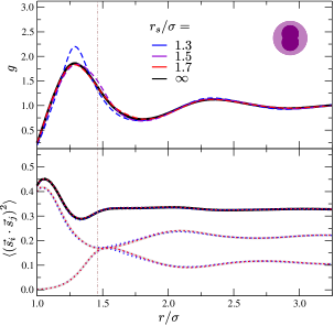
Figure 3: Static correlations for the elementary dumbbell scenario. These molecules have uniform LJ parameters for their two sites, $\sigma$ and $\epsilon$, and the bond length between them is $0.5\sigma$. Here, all the black curves, as well as the gray ones, correspond with the reference system. The colored curves, correspond with the RelRes strategy, with each color representing a different switching distance $r_{s}$. Note particularly the violet curve, which is of the ideal switching distance in capturing the behavior of the reference liquid; the blue or red curve has a shorter or longer switching distance, respectively. Everything is plotted as a function of the distance between the midpoints of the dumbbells, $r$. The top panel plots the corresponding radial distribution $g$, with the solid curve being for the reference system, while the dashed curves being for the RelRes scenarios. The bottom panel, for the reference liquid, plots the orientational correlation $\left\langle\left(\vec{s}_{i}\cdot\vec{s}_{j}\right)^{2}\right\rangle$ as the black curve, together with its two main components $\left\langle\left(s_{i}^{\|}s_{j}^{\|}\right)^{2}\right\rangle$ and $\left\langle\left(s_{i}^{\bot}s_{j}^{\bot}\right)^{2}\right\rangle$ as the lower and higher gray curves, respectively; the functionality of the dotted curves corresponds with the functionality of their neighboring solid curves; note that all of these curves are almost identical. In both panels, the vertical brown line represents the inflection of $g$, which is located here at $1.46$.

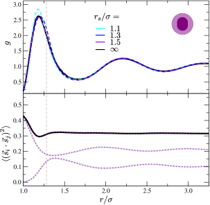
Figure 7: Static correlations for the short dumbbells with a bond length of $0.3\sigma$. Everything here is essentially equivalent with Fig. 3. However, note the cyan curve which is for RelRes with a switching distance of $1.1\sigma$. The vertical line here goes through $1.28$. We plot the orientational function only for $r_{s}=1.5\sigma$, since all other curves are basically identical with it.

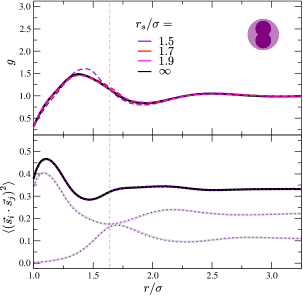
Figure 8: Static correlations for the long dumbbells with a bond length of $0.7\sigma$. Everything here is essentially equivalent with Fig. 3. However, note the magenta curve which is for RelRes with a switching distance of $1.9\sigma$. The vertical line here goes through $1.64$. We plot the orientational function only for $r_{s}=1.5\sigma$, since all other curves are basically identical with it.

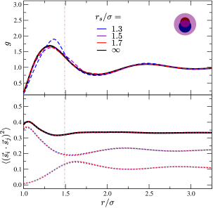
Figure 9: Static correlations for the nonuniform dumbbells, the ones with different LJ parameters across their two sites, $\left\{0.85\sigma,1.18\sigma\right\}$ and $\left\{1.61\epsilon,0.62\epsilon\right\}$. Everything here is essentially equivalent with Fig. 3. The vertical line is at $1.49$.

	Molecule Type	Elementary	Short	Long	Nonuniform
	Bond Length	$0.5$	$0.3$	$0.7$	$0.5$
	Suggested $r_{s}$	$1.5$	$1.3$	$1.7$	$1.5$
	Inflection in $g$	$1.46$	$1.28$	$1.64$	$1.49$
	Midpoint between extrema in $g$	$1.54$	$1.43$	$1.66$	$1.59$
	Inflection in $\left\langle\left(\vec{s}_{i}\cdot\vec{s}_{j}\right)^{2}\right\rangle$	$1.42$	$1.25$	$1.59$	$1.51$
	Maximum in $\left\langle\left(s_{i}^{\|}s_{j}^{\|}\right)^{2}\right\rangle$	$1.49$	$1.36$	$1.64$	$1.57$
	Minimum in $\left\langle\left(s_{i}^{\bot}s_{j}^{\bot}\right)^{2}\right\rangle$	$1.54$	$1.39$	$1.69$	$1.65$

Table 1: Signature distances in the structural correlations of the various dumbbell scenarios. Rows 1-2 give us the molecule type, as well as its respective bond length, which each column corresponds with. Column 2 goes together with Fig. 3, columns 3 and 4 refer to Figs. 7 and 8, respectively, and column 5 goes with Fig. 9. Column 1 then tells us which distance value we are dealing with in each case. Row 3 is the switching distance that we recommend for use in RelRes, based on our systematic examination of varying $r_{s}$. Rows 4-5 deal with signatures of the radial distributions, while rows 6-8 deal with signatures of the orientational functions. Realize that all numbers here are given in units of $\sigma$.

Bibliography

Bibliography

- [1] Aviel Chaimovich, Christine Peter, and Kurt Kremer. Relative resolution: A hybrid formalism for fluid mixtures. The Journal of Chemical Physics, 143(24):243107, 2015.
- [2] C. Jarzynski. Nonequilibrium equality for free energy differences. Physical Review Letters, 78(14):2690–2693, 1997.
- [3] Fugao Wang and D. P. Landau. Efficient, multiple-range random walk algorithm to calculate the density of states. Physical Review Letters, 86(10):2050–2053, 2001.
- [4] Alessandro Laio and Michele Parrinello. Escaping free-energy minima. Proceedings of the National Academy of Sciences of the United States of America, 99(20):12562–12566, 2002.
- [5] Omar Valsson and Michele Parrinello. Variational approach to enhanced sampling and free energy calculations. Physical Review Letters, 113(9):090601, 2014.
- [6] Christoph Dellago, Peter G. Bolhuis, Felix S. Csajka, and David Chandler. Transition path sampling and the calculation of rate constants. The Journal of Chemical Physics, 108(5):1964–1977, 1998.
- [7] Rosalind J. Allen, Patrick B. Warren, and Pieter Rein ten Wolde. Sampling rare switching events in biochemical networks. Physical Review Letters, 94(1):018104, 2005.
- [8] Titus S. van Erp. Reaction rate calculation by parallel path swapping. Physical Review Letters, 98(26):268301, 2007.
- [9] Weinan E, Weiqing Ren, and Eric Vanden-Eijnden. String method for the study of rare events. Physical Review B, 166(5):052301, 2006.
- [10] Victor Ruhle, Christoph Junghans, Alexander Lukyanov, Kurt Kremer, and Denis Andrienko. Versatile object-oriented toolkit for coarse-graining applications. Journal of Chemical Theory and Computation, 5(12):3211–3223, 2009.
- [11] W. G. Noid. Perspective: Coarse-grained models for biomolecular systems. The Journal of Chemical Physics, 139(9):090901, 2013.
- [12] M. Scott Shell. Coarse-graining with the relative entropy. Advances in Chemical Physics, 161(5):395–441, 1964.
- [13] W. G. Noid, Jhih-Wei Chu, Gary S. Ayton, Vinod Krishna, Sergei Izvekov, Gregory A. Voth, Avisek Das, and Hans C. Andersen. The multiscale coarse-graining method. i. a rigorous bridge between atomistic and coarse-grained models. The Journal of Chemical Physics, 128(24):244114, 2008.
- [14] W. G. Noid, Pu Liu, Yanting Wang, Jhih-Wei Chu, Gary S. Ayton, Sergei Izvekov, Hans C. Andersen, and Gregory A. Voth. The multiscale coarse-graining method. ii. numerical implementation for coarse-grained molecular models. The Journal of Chemical Physics, 128(24):244115, 2008.
- [15] R. L. Henderson. A uniqueness theorem for fluid pair correlation functions. Physics Letters A, 49(3):197–198, 1974.
- [16] R. L. McGreevy and L. Pusztai. Reverse monte carlo simulation: A new technique for the determination of disordered structures. Molecular Simulation, 1(6):359–367, 1988.
- [17] Teresa Head-Gordon and Frank H. Stillinger. An orientational perturbation theory for pure liquid water. The Journal of Chemical Physics, 98(4):3313–3327, 1993.
- [18] Alexander P. Lyubartsev and Aatto Laaksonen. Calculation of effective interaction potentials from radial distribution functions: A reverse monte carlo approach. Physical Review E, 52(4):3730–3737, 1995.
- [19] Reith Dirk, Putz Mathias, and Muller-Plathe Florian. Deriving effective mesoscale potentials from atomistic simulations. The Journal of Computational Chemistry, 24(13):1624–1636, 2003.
- [20] J. W. Mullinax and W. G. Noid. Generalized yvon-born-green theory for molecular systems. Physical Review Letters, 103(19):198104, 2009.
- [21] John G. Kirkwood. Statistical mechanics of fluid mixtures. The Journal of Chemical Physics, 3(5):300–313, 1935.
- [22] A. A. Louis. Beware of density dependent pair potentials. Journal of Physics: Condensed Matter, 14(40):9187–9206, 2002.
- [23] Christine Peter and Kurt Kremer. Multiscale simulation of soft matter systems. Faraday Discussions, 144(0):9–24, 2010.
- [24] Marilisa Neri, Claudio Anselmi, Michele Cascella, Amos Maritan, and Paolo Carloni. Coarse-grained model of proteins incorporating atomistic detail of the active site. Physical Review Letters, 95(21):218102, 2005.
- [25] Qiang Shi, Sergei Izvekov, and Gregory A. Voth. Mixed atomistic and coarse-grained molecular dynamics: Simulation of a membrane-bound ion channel. The Journal of Physical Chemistry B, 110(31):15045–15048, 2006.
- [26] Andrzej J. Rzepiela, Martti Louhivuori, Christine Peter, and Siewert J. Marrink. Hybrid simulations: combining atomistic and coarse-grained force fields using virtual sites. Physical Chemistry Chemical Physics, 13(22):10437–10448, 2011.
- [27] Wei Han and Klaus Schulten. Further optimization of a hybrid united-atom and coarse-grained force field for folding simulations: Improved backbone hydration and interactions between charged side chains. Journal of Chemical Theory and Computation, 8(11):4413–4424, 2012.
- [28] V. A. Harmandaris, N. P. Adhikari, N. F. A. van der Vegt, and K. Kremer. Hierarchical modeling of polystyrene: From atomistic to coarse-grained simulations. Macromolecules, 39(19):6708–6719, 2006.
- [29] Theodora Spyriouni, Christos Tzoumanekas, Doros Theodorou, Florian Muller-Plathe, and Giuseppe Milano. Coarse-grained and reverse-mapped united-atom simulations of long-chain atactic polystyrene melts: Structure, thermodynamic properties, chain conformation, and entanglements. Macromolecules, 40(10):3876–3885, 2007.
- [30] Edward Lyman, F. Marty Ytreberg, and Daniel M. Zuckerman. Resolution exchange simulation. Physical Review Letters, 96(2):028105, 2006.
- [31] Markus Christen and Wilfred F. van Gunsteren. Multigraining: An algorithm for simultaneous fine-grained and coarse-grained simulation of molecular systems. The Journal of Chemical Physics, 124(15):154106, 2006.
- [32] Matej Praprotnik, Luigi Delle Site, and Kurt Kremer. Adaptive resolution molecular-dynamics simulation: Changing the degrees of freedom on the fly. The Journal of Chemical Physics, 123(22):224106, 2005.
- [33] Cameron F. Abrams. Concurrent dual-resolution monte carlo simulation of liquid methane. The Journal of Chemical Physics, 123(23):234101, 2005.
- [34] Bernd Ensing, Steven O. Nielsen, Preston B. Moore, Michael L. Klein, and Michele Parrinello. Energy conservation in adaptive hybrid atomistic/coarse-grain molecular dynamics. Journal of Chemical Theory and Computation, 3(3):1100–1105, 2007.
- [35] Raffaello Potestio, Sebastian Fritsch, Pep Espanol, Rafael Delgado-Buscalioni, Kurt Kremer, Ralf Everaers, and Davide Donadio. Hamiltonian adaptive resolution simulation for molecular liquids. Physical Review Letters, 110(10):108301, 2013.
- [36] Julija Zavadlav, Manuel Nuno Melo, Siewert J. Marrink, and Matej Praprotnik. Adaptive resolution simulation of an atomistic protein in martini water. The Journal of Chemical Physics, 140(5):054114, 2014.
- [37] Aoife C. Fogarty, Raffaello Potestio, and Kurt Kremer. Adaptive resolution simulation of a biomolecule and its hydration shell: Structural and dynamical properties. The Journal of Chemical Physics, 142(19):195101, 2015.
- [38] Sergei Izvekov and Gregory A. Voth. Mixed resolution modeling of interactions in condensed-phase systems. Journal of Chemical Theory and Computation, 5(12):3232–3244, 2009.
- [39] Lin Shen and Hao Hu. Resolution-adapted all-atomic and coarse-grained model for biomolecular simulations. Journal of Chemical Theory and Computation, 10(6):2528–2536, 2014.
- [40] H. L. Frisch. The equation of state of the classical hard sphere fluid. Advances in Chemical Physics, 6(5):229–289, 1964.
- [41] B. Widom. Intermolecular forces and the nature of the liquid state: Liquids reflect in their bulk properties the attractions and repulsions of their constituent molecules. Science, 157(3787):375–382, 1967.
- [42] John D. Weeks, David Chandler, and Hans C. Andersen. Role of repulsive forces in determining the equilibrium structure of simple liquids. The Journal of Chemical Physics, 54(12):5237–5247, 1971.
- [43] Trond S. Ingebrigtsen, Thomas B. Schroder, and Jeppe C. Dyre. What is a simple liquid? Physical Review X, 2(1):011011, 2012.
- [44] Berk Hess, Carsten Kutzner, David van der Spoel, and Erik Lindahl. Gromacs 4: Algorithms for highly efficient, load-balanced, and scalable molecular simulation. Journal of Chemical Theory and Computation, 4(3):435–447, 2008.
- [45] L. Greengard and V. Rokhlin. A fast algorithm for particle simulations. Journal of Computational Physics, 73(2):325–348, 1987.
- [46] Jason A. Wagoner and Vijay S. Pande. A smoothly decoupled particle interface: New methods for coupling explicit and implcit solvent. The Journal of Chemical Physics, 134(21):214103, 2011.
- [47] Dmitrii Beglov and Benoit Roux. Finite representation of an infinite bulk system: Solvent boundary potential for computer simulations. The Journal of Chemical Physics, 100(12):9050–9063, 1994.