Magnus-type integrator for the finite element discretization of semilinear parabolic non-autonomous SPDEs driven by additive noise

Abstract.

In this paper, we investigate a numerical approximation of a general second order semilinear parabolic non-autonomous stochastic partial differential equation (SPDE) driven by additive noise. Numerical approximations for autonomous SPDEs are thoroughly investigated in the literature while the non-autonomous case is not yet well understood. We discretize the non-autonomous SPDE in space by the finite element method and in time by the Magnus-type integrator. We provide a strong convergence proof of the fully discrete scheme toward the mild solution in the root-mean-square $L^{2}$ norm. Appropriate assumptions on the drift term and the noise allow to achieve optimal convergence order in time greater than $1/2$, without any logarithmic reduction of convergence order in time. In particular, for trace class noise, we achieve optimal convergence orders $\mathcal{O}\left(h^{2-\epsilon}+\Delta t\right)$, where $\epsilon$ is a positive number small enough. Numerical simulations are provided to illustrate our theoretical results.

Dans ce papier, nous investigons l’approximation numérique d‘equations aux derivées partielles (EDP) stochastique sémilinéaire et non autonome avec un bruit additif. L’approximation numérique d’EPD stochastique autonome est largement étudiée dans la littérature scientifique, tandis que le cas non autonome reste encore trés peu connu. Le but de ce papier est d‘investiguer le cas non autonome avec un bruit additif. L’EDP stochastique est discretisée en espace par la méthode des élements finis et en temps par un schema exponentiel de type Magnus. En plus, sous des hypothèses appropriés, nous obtenons un ordre de convergence en temps supérieur a $1/2$, sans aucune reduction logarithmique. En particulier, pour un bruit de trace fini, nous obtenons une convergence de la forme $\mathcal{O}\left(h^{2-\epsilon}+\Delta t\right)$, où $\epsilon$ est un nombre réel positif et suffisament petit. Les simulations numériques pour illustrer les résultats théoriques sont aussi faites.

Introduction

We consider the numerical approximations of the following semilinear parabolic non-autonomous SPDE driven by additive noise

$$dX(t)=[A(t)X(t)+F\left(t,X(t)\right)]dt+dW(t),\quad X(0)=X_{0},\quad t\in(0,T],$$ (1)

in the Hilbert space $L^{2}(\Lambda)$, where $\Lambda$ is a bounded domain of $\mathbb{R}^{d}$, $d=1,2,3$ and $T>0$. The family of the unbounded linear operators $A(t)$ are not necessarily self-adjoint. Each $A(t)$ is assumed to generate an analytic semigroup $S_{t}(s):=e^{A(t)s}$. Precise assumptions on $A(t)$ and $F$ to ensure the existence of the unique mild solution of (1) are given in the next section. The random initial data is denoted by $X_{0}$. We denote by $(\Omega,\mathcal{F},\mathbb{P})$ a probability space with a filtration $(\mathcal{F}_{t})_{t\in[0,T]}\subset\mathcal{F}$ that fulfills the usual conditions, see e.g., [34, Definition 2.1.11]. The noise term $W(t)$ is assumed to be a $Q$-Wiener process defined on a filtered probability space $(\Omega,\mathcal{F},\mathbb{P},\{\mathcal{F}_{t}\}_{t\in[0,T]})$, where the covariance operator $Q:H\longrightarrow H$ is assumed to be linear, self adjoint and positive definite. It is well known (see e.g., [34]) that the noise can be represented as

$$W(t,x)=\sum_{i=0}^{\infty}\sqrt{q}_{i}e_{i}(x)\beta_{i}(t),$$ (2)

where $(q_{i},e_{i})_{i\in\mathbb{N}}$ are the eigenvalues and eigenfunctions of the covariance operator $Q$, and $(\beta_{i})_{i\in\mathbb{N}}$ are independent and identically distributed standard Brownian motion. Autonomous systems are not realistic to model phenomena in many fields such as quantum fields theory, electromagnetism, nuclear physics, see e.g., [3, Section 7] and references therein. Numerical solutions of (1) based on implicit, explicit Euler methods and exponential integrators with $A(t)=A$, where $A$ is selfadjoint are thoroughly investigated in the literature, see e.g., [15, 19, 44, 26]. If we turn our attention to the case of $A(t)=A$, with $A$ not necessary self adjoint, the list of references become remarkably short, see e.g., [25, 30]. The numerical approximation in time of the deterministic counter part of (1) with time dependent coefficient $A(t)$ was investigated in [9, 12, 13, 38], where Magnus-type integrator [28] was used in [9, 13, 38]; and a new exponential integrator was used in [12]. Numerical approximation for non-autonomous SPDE (1) is not yet well understood due to the complexity of the linear operator $A(t)$ and its semigroup $S_{t}(s)=e^{A(t)s}$. Recently numerical scheme for stochastic model (1) driven by multiplicative noise with time dependent linear operator $A(t)$ was investigated in [39], where the time discretization was done using the Magnus-type integrator. The optimal convergence order in time in [39] was $1/2$. This is the optimal convergence order when dealing with multiplicative noise with schemes based on Euler approximations (namely explicit Euler method, linear implicit Euler method, exponential Euler, exponential Rosenbrock-Euler). In fact even for stochastic ordinary differential equation (SODE) driven by multiplicative noise, the Euler type method achieves optimal order $1/2$, see e.g., [2], whereas when dealing with SODE driven by additive noise the optimal convergence order is $1$, see e.g. [18]. In this paper, we extend that result to the SPDE (1) and prove that the Magnus-type integrator applied to SPDE (1) achieves an optimal order $1$ in time. The price to pay is that we require additional assumptions on the nonlinear function $F$ than the only standard Lipschitz condition. An important ingredient to achieve that optimal convergence order is the application of Taylor’s formula in Banach space to the drift function, see TalyorBanach. It is worth to mention that such approach and assumptions on the nonlinear drift function $F$ were also used in [17, 44, 30, 26] for exponential integrators and semi-implicit Euler method for autonomous SPDEs driven by additive noise to achieve optimal convergence order $1$ in time. Due to the complexity of the linear operator and the corresponding semi discrete linear operator after space discretisation, novel additional technical estimates are provided on the terms involving the noise to achieve higher convergence order, see e.g., fonda and Noiseestimate. The result indicates how the convergence orders depend on the regularity of the initial data and the noise. More precisely, the fully discrete scheme achieves convergence order $\mathcal{O}\left(h^{\beta}+\Delta t^{\beta/2}\right)$, where $\beta$ is defined in assumption1. We emphasize that comparing with results for autonomous SPDES with not necessary self adjoint, here we achieve optimal convergence order $1$ in time for the border case $\beta=2$, instead of sub-optimal convergence order $1-\epsilon$ obtained in [30, 15]. The optimal convergence orders achieved in [43, 19, 44], where due to sharp integral estimates and optimal regularity estimates in [20]. Note that key ingredient to achieve optimal regularity estimates in [20] is the spectral decomposition of the linear operator $A$. This cannot directly applied to the case of time dependent and not necessarily self-adjoint operator $A(t)$ due to its complexity and its associated semigroup $S_{s}(t)=e^{A(s)t}$. In this paper, sharp and 2.11 provide appropriate ingredients to fill the gap.

The rest of this paper is organised as follows. wellposed provides the general setting, the numerical scheme and the main result. In convergenceproof, we provide some preparatory results and present the proof of the main results. experiment provides some numerical experiments to sustain our theoretical results.

1. Mathematical setting, numerical scheme and main results

1.1. Notations and main assumptions

Let $(H,\langle.,.\rangle_{H},\|.\|)$ be an separable Hilbert space. For all $p\geq 2$ and for a Banach space $U$, we denote by $L^{p}(\Omega,U)$ the Banach space of all equivalence classes of $p$ integrable $U$-valued random variables. Let $L(U,H)$ be the space of bounded linear mappings from $U$ to $H$ endowed with the usual operator norm $\|.\|_{L(U,H)}$. By $\mathcal{L}_{2}(U,H):=HS(U,H)$, we denote the space of Hilbert-Schmidt operators from $U$ to $H$ equipped with the norm $\|l\|^{2}_{\mathcal{L}_{2}(U,H)}:=\sum\limits_{i=1}^{\infty}\|l\psi_{i}\|^{2}$, $l\in\mathcal{L}_{2}(U,H)$, where $(\psi_{i})_{i=1}^{\infty}$ is an orthonormal basis of $U$. Note that this definition is independent of the orthonormal basis of $U$. For simplicity, we use the notations $L(U,U)=:L(U)$ and $\mathcal{L}_{2}(U,U)=:\mathcal{L}_{2}(U)$. For all $l\in L(U,H)$ and $l_{1}\in\mathcal{L}_{2}(U)$ we have $ll_{1}\in\mathcal{L}_{2}(U,H)$ and

$$\|ll_{1}\|_{\mathcal{L}_{2}(U,H)}\leq\|l\|_{L(U,H)}\|l_{1}\|_{\mathcal{L}_{2}(U)},$$ (3)

see e.g., [5]. The covariance operator $Q:H\longrightarrow H$ is assumed to be positive and self-adjoint. Throughout this paper $W(t)$ is a $Q$-wiener process. The space of Hilbert-Schmidt operators from $Q^{1/2}(H)$ to $H$ is denoted by $L^{0}_{2}:=\mathcal{L}_{2}(Q^{1/2}(H),H)=HS(Q^{1/2}(H),H)$. As usual, $L^{0}_{2}$ is equipped with the norm

$$\|l\|_{L^{0}_{2}}:=\|lQ^{1/2}\|_{HS}=\left(\sum\limits_{i=1}^{\infty}\|lQ^{1/2}e_{i}\|^{2}\right)^{1/2},\quad l\in L^{0}_{2},$$ (4)

where $(e_{i})_{i=1}^{\infty}$ is an orthonormal basis of $H$. This definition is independent of the orthonormal basis of $H$. For an $L^{0}_{2}$- predictable stochastic process $\phi:[0,T]\times\Lambda\longrightarrow L^{0}_{2}$ such that

$$\int_{0}^{t}\mathbb{E}\left\|\phi(s)Q^{1/2}\right\|^{2}_{\mathcal{L}_{2}(H)}ds<\infty,\quad t\in[0,T],$$ (5)

the following relation called Itô’s isometry property holds

$$\mathbb{E}\left\|\int_{0}^{t}\phi(s)dW(s)\right\|^{2}=\int_{0}^{t}\mathbb{E}\left\|\phi(s)\right\|^{2}_{L^{0}_{2}}ds=\int_{0}^{t}\mathbb{E}\left\|\phi(s)Q^{1/2}\right\|^{2}_{\mathcal{L}_{2}(H)}ds,\quad t\in[0,T],$$ (6)

see e.g., [33, Step 2 in Section 2.3.2] or [34, Proposition 2.3.5].

In the rest of this paper, we consider $H=L^{2}(\Lambda)$. To guarantee the existence of a unique mild solution of (1) and for the purpose of the convergence analysis, we make the following assumptions. The initial data $X_{0}:\Omega\longrightarrow H$ is assumed to be measurable and $X_{0}\in L^{4}\left(\Omega,\mathcal{D}\left((-A(0))^{\beta/2}\right)\right)$, $0\leq\beta\leq 2$. We equip $V_{\alpha}(t):=\mathcal{D}\left((-A(t))^{\alpha/2}\right)$, $\alpha\in\mathbb{R}$ with the norm $\|u\|_{\alpha,t}:=\|(-A(t))^{\alpha/2}u\|$. Due to (14), (15) and for the seek of ease notations, we simply write $V_{\alpha}$ and $\|.\|_{\alpha}$. We follow [36, 44, 30, 43] and assume that the nonlinear operator $F$ satisfies the following Lipschitz condition. The nonlinear operator $F:[0,T]\times H\longrightarrow H$ is assumed to be $\beta/2$-Hölder continuous with respect to the first variable and Lipschitz continuous with respect to the second variable, i.e. there exists a positive constant $K_{3}$ such that

$$\|F(s,0)\|\leq K_{3},\quad\|F(t,u)-F(s,v)\|\leq K_{3}\left(|t-s|^{\beta/2}+\|u-v\|\right),\quad s,t\in[0,T],\quad u,v\in H.$$ (7)

We also assume the drift function to be twice differentiable with bounded derivative, i.e. there exists a constant $K_{1}>0$ such that

$$\|F^{\prime}(t,v)\|_{L(H)} \leq K_{1},\quad\forall\,v\in H,\quad t\in[0,T]$$ (8)

$$\|F^{\prime\prime}(t,u)(v_{1},v_{2})\|_{-\eta} \leq K_{1}\|v_{1}\|.\|v_{2}\|,\quad u,v_{1},v_{2}\in H,\quad\text{for some }\,\eta\in[1,2),\quad t\in[0,T],$$ (9)

where the Fréchet first and second order derivatives are taken respect to the second variable. We assume the covariance operator $Q:H\longrightarrow H$ to satisfy

$$\left\|(-A(0))^{\frac{\beta-1}{2}}Q^{\frac{1}{2}}\right\|_{\mathcal{L}_{2}(H)}<\infty,$$ (10)

where $\beta$ is defined in Assumption 1.1. As in [9, 12, 10], we make the following assumptions on the family of linear operator $A(t)$.

• We assume that $\mathcal{D}\left(A(t)\right)=D$, $0\leq t\leq T$ and the family of linear operators $A(t):D\subset H\longrightarrow H$ to be uniformly sectorial on $0\leq t\leq T$, i.e. there exist constants $c>0$ and $\theta\in\left(\frac{1}{2}\pi,\pi\right)$ such that

  $$\left\|\left(\lambda\mathbf{I}-A(t)\right)^{-1}\right\|_{L(L^{2}(\Lambda))}\leq\frac{c}{|\lambda|},\quad\lambda\in S_{\theta},$$ (11)

  where $S_{\theta}:=\left\{\lambda\in\mathbb{C}:\lambda=\rho e^{i\phi},\rho>0,0\leq|\phi|\leq\theta\right\}$. As in [12], by a standard scaling argument, we assume $-A(t)$ to be invertible with bounded inverse.

• We require the following Lipschitz conditions respect to the time

  $$\left\|\left(A(t)-A(s)\right)(-A(0))^{-1}\right\|_{L(H)} \leq K_{1}|t-s|,\quad s,t\in[0,T],$$ (12)

  $$\left\|(-A(0))^{-1}\left(A(t)-A(s)\right)\right\|_{L(D,H)} \leq K_{1}|t-s|,\quad s,t\in[0,T].$$ (13)

• As we are dealing with non smooth data, we follow [36] and assume that

  $$\mathcal{D}\left(\left(-A(t)\right)^{\alpha}\right)=\mathcal{D}\left(\left(-A(0)\right)^{\alpha}\right),\quad 0\leq t\leq T,\quad 0\leq\alpha\leq 1$$ (14)

  and there exists a positive constant $K_{2}$ such that the following estimate holds

  $$K_{2}^{-1}\left\|\left(-A(0)\right)^{\alpha}u\right\|\leq\left\|(-A(t))^{\alpha}u\right\|\leq K_{2}\left\|(-A(0))^{\alpha}u\right\|,\quad t\in[0,T],\quad u\in\mathcal{D}((-A(0))^{\alpha}).$$ (15)

Remark 1.1.

As a consequence of Assumption 1.1, for all $\alpha\geq 0$ and $\gamma\in[0,1]$, there exists a constant $C_{1}\geq 0$ such that the following estimate holds uniformly in $t\in[0,T]$

$$\left\|(-A(t))^{\alpha}e^{sA(t)}\right\|_{L(H)}\leq C_{1}s^{-\alpha},s>0,$$ (16)

$$\left\|(-A(t))^{-\gamma}\left(\mathbf{I}-e^{sA(t)}\right)\right\|_{L(H)}\leq C_{1}s^{\gamma},\quad s\geq 0.$$ (17)

Proposition 1.2.

Let $\Delta(T):=\{(t,s):0\leq s\leq t\leq T\}$. Under assumption2 there exists a unique evolution system [32, Definition 5.3, Chapter 5] $U:\Delta(T)\longrightarrow L(H)$ such that

• There exists a positive constant $K_{0}$ such that

  $$\|U(t,s)\|_{L(H)}\leq K_{0},\quad 0\leq s\leq t\leq T.$$ (18)

• $U(.,s)\in C^{1}(]s,T];L(H))$, $0\leq s\leq T$,

  $$\frac{\partial U}{\partial t}(t,s)=-A(t)U(t,s)\quad\text{and}\quad\|A(t)U(t,s)\|_{L(H)}\leq\frac{K_{0}}{t-s},\quad 0\leq s<t\leq T.$$ (19)

• $U(t,.)x\in C^{1}([0,t[;H)$, $0<t\leq T$, $x\in\mathcal{D}(A(0))$ and

  $$\frac{\partial U}{\partial s}(t,s)=-U(t,s)A(s)x\quad\text{and}\quad\|A(t)U(t,s)A(s)^{-1}\|_{L(H)}\leq K_{0},\quad 0\leq s\leq t\leq T.$$ (20)

Proof 1.3.

See [32, Theorem 6.1, Chapter 5].

Theorem 1.4.

Let assumption1, 1.1 and 1.1 (i)-(ii) be fulfilled. Then the non-autonomous problem (1) has a unique mild solution $X(t)$, which takes the following form

$$X(t)=U(t,0)X_{0}+\int_{0}^{t}U(t,s)F(s,X(s))ds+\int_{0}^{t}U(t,s)dW(s),$$ (21)

where $U(t,s)$ is the evolution system of proposition1. Moreover, there exists a positive constant $K_{4}$ such that

$$\sup_{0\leq t\leq T}\|X(t)\|_{L^{2}\left(\Omega,\mathcal{D}((-A(0))^{\beta/2}))\right)}\leq K_{4}\left(1+\|X_{0}\|_{L^{2}\left(\Omega,\mathcal{D}((-A(0))^{\beta/2}\right)}\right).$$ (22)

Proof 1.5.

See [36, Theorem 1.3].

1.2. Fully discrete scheme and main result

In the rest of this paper, we consider the family of linear operators $A(t)$ to be of second order of the following form

$$A(t)u=\sum_{i,j=1}^{d}\frac{\partial}{\partial x_{i}}\left(q_{ij}(x,t)\frac{\partial u}{\partial x_{j}}\right)-\sum_{j=1}^{d}q_{j}(x,t)\frac{\partial u}{\partial x_{j}}.$$ (23)

We require the coefficients $q_{i,j}$ and $q_{j}$ to be smooth functions on the variable $x\in\overline{\Lambda}$ and Hölder-continuous with respect to $t\in[0,T]$. We further assume that there exists a positive constant $c_{1}$ such that the following ellipticity condition holds

$$\sum_{i,j=1}^{d}q_{ij}(x,t)\xi_{i}\xi_{j}\geq c_{1}|\xi|^{2},\quad(x,t)\in\overline{\Lambda}\times[0,T].$$ (24)

Under the above assumptions on $q_{ij}$ and $q_{j}$, it is well known that the family of linear operators defined in (23) fulfills assumption2 (i)-(ii) with $D=H^{2}(\Lambda)\cap H^{1}_{0}(\Lambda)$, see [32, Section 7.6] or [41, Section 5.2]. The above assumptions on $q_{ij}$ and $q_{j}$ also imply that assumption2 (iii) is fulfilled, see e.g., [36, Example 6.1] or [1, 35].

As in [8, 25], we introduce two spaces $\mathbb{H}$ and $V$, such that $\mathbb{H}\subset V$, that depend on the boundary conditions for the domain of the operator $-A(t)$ and the corresponding bilinear form. For example, for Dirichlet boundary conditions we take

$$V=\mathbb{H}=H^{1}_{0}(\Lambda)=\{v\in H^{1}(\Lambda):v=0\quad\text{on}\quad\partial\Lambda\}.$$ (25)

For Robin boundary condition and Neumann boundary condition, which is a special case of Robin boundary condition ($\alpha_{0}=0$), we take $V=H^{1}(\Lambda)$ and

$$\mathbb{H}=\{v\in H^{2}(\Lambda):\partial v/\partial v_{A}+\alpha_{0}v=0,\quad\text{on}\quad\partial\Lambda\},\quad\alpha_{0}\in\mathbb{R}.$$ (26)

Using Green’s formula and the boundary conditions, we obtain the corresponding bilinear form associated to $-A(t)$

$$a(t)(u,v)=\int_{\Lambda}\left(\sum_{i,j=1}^{d}q_{ij}(x,t)\dfrac{\partial u}{\partial x_{i}}\dfrac{\partial v}{\partial x_{j}}+\sum_{i=1}^{d}q_{i}(x,t)\dfrac{\partial u}{\partial x_{i}}v\right)dx,\quad u,v\in V,$$ (27)

for Dirichlet boundary conditions and

$$a(t)(u,v)=\int_{\Lambda}\left(\sum_{i,j=1}^{d}q_{ij}(x,t)\dfrac{\partial u}{\partial x_{i}}\dfrac{\partial v}{\partial x_{j}}+\sum_{i=1}^{d}q_{i}(x,t)\dfrac{\partial u}{\partial x_{i}}v\right)dx+\int_{\partial\Lambda}\alpha_{0}uvdx,\quad u,v\in V.$$ (28)

for Robin and Neumann boundary conditions. Using Gårding’s inequality, it holds that there exist two constants $\lambda_{0}$ and $c_{0}$ such that

$$a(t)(v,v)\geq\lambda_{0}\|v\|^{2}_{1}-c_{0}\|v\|^{2},\quad v\in V,\quad t\in[0,T].$$ (29)

By adding and subtracting $c_{0}u$ on the right hand side of (1), we obtain a new family of linear operators that we still denote by $A(t)$. Therefore the new corresponding bilinear form associated to $-A(t)$ still denoted by $a(t)$ satisfies the following coercivity property

$$a(t)(v,v)\geq\;\lambda_{0}\|v\|_{1}^{2},\;\;\;\;\;v\in V,\quad t\in[0,T].$$ (30)

Note that the expression of the nonlinear term $F$ has changed as we have included the term $-c_{0}u$ in the new nonlinear term that we still denote by $F$.

The coercivity property (30) implies that $A(t)$ and $A_{h}(t)$ are sectorial on $L^{2}(\Lambda)$ (uniformly in $h$), see e.g., [23]. Therefore $A_{h}(t)$ and $A(t)$ generate analytic semigroups denoted respectively by $S_{h,t}(s):=e^{sA_{h}(t)}$ and $S_{t}(s)=e^{sA(t)}$ on $L^{2}(\Lambda)$ such that [11]

$$S_{t}(s)=e^{sA(t)}=\dfrac{1}{2\pi i}\int_{\mathcal{C}}e^{s\lambda}(\lambda I-A(t))^{-1}d\lambda,\;\;\;\;\;\;\;\;s>0,$$ (31)

where $\mathcal{C}$ denotes a path that surrounds the spectrum of $A(t)$. The coercivity property (30) also implies that $-A(t)$ is a positive operator and its fractional powers are well defined and for any $\alpha>0$, we have

$$\left\{\begin{array}[]{rcl}(-A(t))^{-\alpha}&=&\frac{1}{\Gamma(\alpha)}\displaystyle\int_{0}^{\infty}s^{\alpha-1}{\rm e}^{sA(t)}ds,\\ (-A(t))^{\alpha}&=&((-A(t))^{-\alpha})^{-1},\end{array}\right.$$ (32)

where $\Gamma(\alpha)$ is the Gamma function [11]. The domain of $(-A(t))^{\alpha/2}$ are characterized in [8, 6, 23] for $1\leq\alpha\leq 2$ with equivalence of norms as follows

$$\mathcal{D}((-A(t))^{\alpha/2})=H^{1}_{0}(\Lambda)\cap H^{\alpha}(\Lambda)\hskip 28.45274pt\text{(for Dirichlet boundary condition)}$$

$$\mathcal{D}(-A(t))=\mathbb{H},\quad\mathcal{D}((-A(t))^{1/2})=H^{1}(\Lambda)\hskip 14.22636pt\text{(for Robin boundary condition)}$$

$$\|v\|_{H^{\alpha}(\Lambda)}\equiv\|((-A(t))^{\alpha/2}v\|:=\|v\|_{\alpha},\quad\forall v\in\mathcal{D}((-A(t))^{\alpha/2}).$$

The characterization of $\mathcal{D}((-A(t))^{\alpha/2})$ for $0\leq\alpha<1$ can be found in [31, Theorem 2.1 & Theorem 2.2].

Now, we turn our attention to the discretization of the problem (1). We start by splitting the domain $\Lambda$ in finite triangles. Let $\mathcal{T}_{h}$ be the triangulation with maximal length $h$ satisfying the usual regularity assumptions, and $V_{h}\subset V$ be the space of continuous functions that are piecewise linear over the triangulation $\mathcal{T}_{h}$. We consider the projection $P_{h}$ from $H=L^{2}(\Lambda)$ to $V_{h}$ defined for every $u\in H$ by

$$\langle P_{h}u,\chi\rangle_{H}=\langle u,\chi\rangle_{H},\quad\phi,\chi\in V_{h}.$$ (33)

For all $t\in[0,T]$, the discrete operator $A_{h}(t):V_{h}\longrightarrow V_{h}$ is defined by

$$\langle A_{h}(t)\phi,\chi\rangle_{H}=\langle A(t)\phi,\chi\rangle_{H}=-a(t)(\phi,\chi),\quad\phi,\chi\in V_{h}.$$ (34)

The coercivity property (30) implies that there exist constants $C_{2}>0$ and $\theta\in(\frac{1}{2}\pi,\pi)$ such that

$$\|(\lambda\mathbf{I}-A_{h}(t))^{-1}\|_{L(H)}\leq\frac{C_{2}}{|\lambda|},\quad\lambda\in S_{\theta}$$ (35)

holds uniformly for $h>0$ and $t\in[0,T]$. See e.g., [23] (2.9) or [8, 11]. The coercivity property (30) also implies that the smooth properties (16) and (17) hold for $A_{h}$ uniformly on $h>0$ and $t\in[0,T]$, i.e. for all $\alpha\geq 0$ and $\gamma\in[0,1]$, there exist a positive constant $C_{3}$ such that the following estimates hold uniformly on $h>0$ and $t\in[0,T]$, see e.g. [8, 11]

$$\left\|(-A_{h}(t))^{\alpha}e^{sA_{h}(t)}\right\|_{L(H)}\leq C_{3}s^{-\alpha},\quad s>0,$$ (36)

$$\left\|(-A_{h}(t))^{-\gamma}\left(\mathbf{I}-e^{sA_{h}(t)}\right)\right\|_{L(H)}\leq C_{3}s^{\gamma},\quad s\geq 0.$$ (37)

The semi-discrete version of (1) consists of finding $X^{h}(t)\in V_{h}$, $t\in[0,T]$ such that

$$dX^{h}(t)=\left[A_{h}(t)X^{h}(t)+P_{h}F\left(t,X^{h}(t)\right)\right]dt+P_{h}dW(t),\quad t\in(0,T],\quad X^{h}(0)=P_{h}X_{0}.$$ (38)

Throughout this paper we take $t_{m}=m\Delta t\in[0,T]$, where $T=M\Delta t$ for $m,M\in\mathbb{N}$, $m\leq M$. Following [39], we have the following fully discrete scheme for (1), called stochastic Magnus-type integrator (SMTI) for SPDEs

$$X^{h}_{m+1}=e^{\Delta tA_{h,m}}X^{h}_{m}+\Delta t\varphi_{1}(\Delta tA_{h,m})P_{h}F\left(t_{m},X^{h}_{m}\right)+e^{\Delta tA_{h,m}}P_{h}\Delta W_{m},\quad m\geq 0,\quad X^{h}_{0}=P_{h}X_{0},$$ (39)

where $\Delta W_{m}:=W_{(m+1)\Delta t}-W_{m\Delta t}$, $A_{h,m}:=A_{h}(t_{m})$ and the linear operator $\varphi_{1}(\Delta tA_{h,m})$ is given by

$$\varphi_{1}(\Delta tA_{h,m}):=\dfrac{1}{\Delta t}\int_{0}^{\Delta t}e^{(\Delta t-s)A_{h,m}}ds.$$ (40)

Note that the numerical scheme (39) can be written in the following integral form, useful for the error analysis

$$X^{h}_{m+1}=e^{\Delta tA_{h,m}}X^{h}_{m}+\int_{t_{m}}^{t_{m+1}}e^{(t_{m+1}-s)A_{h,m}}P_{h}F\left(t_{m},X^{h}_{m}\right)ds+\int_{t_{m}}^{t_{m+1}}e^{\Delta tA_{h,m}}P_{h}dW(s).$$ (41)

Note also that an equivalent formulation of the numerical scheme (39), easy for simulation is given by

$$X^{h}_{m+1}=X^{h}_{m}+P_{h}\Delta W_{m}+\Delta t\varphi_{1}(\Delta tA_{h,m})\left[A_{h,m}\left(X^{h}_{m}+P_{h}\Delta W_{m}\right)+P_{h}F\left(t_{m},X^{h}_{m}\right)\right].$$ (42)

The following assumption will be needed in our convergence estimate to achieve optimal convergence order in time without any logarithmic reduction. Let $A(t)=A^{s}(t)+A^{ns}(t)$, where $A^{s}(t)$ and $A^{ns}(t)$ are respectively the self-adjoint and the non self-adjoint parts of $A(t)$. We assume that the family $(\lambda_{n}(t))_{n\in\mathbb{N}}$ of positive eigenvalues of $-A^{s}(t)$ corresponding to the eigenvectors $(e_{n}(t))_{n\in\mathbb{N}}$ are such that for $x\in H$

$$\underset{0\leq t\leq T}{\sup}\lambda_{n}(t)<C(n),\,\quad\underset{0\leq t\leq T}{\sup}(e_{n}(t),x)<C_{1}(x,n).$$ (43)

where $C(n)$ and $C_{1}=C_{1}(x,n)$ are two positive constants.

Remark 1.6.

Typical examples which fulfilled Assumption 1.2 are linear operators $A(t)$ defined in (23) with bounded coefficients such that $q_{ii}(x,t)>0$ and $q_{ij}(x,t)=0,\,\,i\neq j$ with (43). Note that assumption5 coincides with the assumptions made in [20, 19, 43] on the constant self-adjoint operator $A$, where the authors also achieved optimal convergence orders. Note that these optimal convergence orders were due to the sharp integral estimate [20]. In the case of non-autonomous and non necessarily self adjoint operator, sharp and 2.11 are keys ingredients to achieve optimal convergence orders with no reduction.

In the rest of this paper $C$ denotes a generic constant that may change from one place to another. The numerical method being built, we can now state its strong convergence result toward the mild solution, which is the main result of this work.

Theorem 1.7.

[Main result] Let assumption1-1.1 and 1.2 be fulfilled. Then the following error estimate holds

• If $0\leq\beta<2$ then

  $$\left(\mathbb{E}\|X(t_{m})-X^{h}_{m}\|^{2}\right)^{1/2}\leq C\left(h^{\beta}+\Delta t^{\beta/2}\right).$$ (44)

• If $\beta=2$ then

  $$\left(\mathbb{E}\|X(t_{m})-X^{h}_{m}\|^{2}\right)^{1/2}\leq C\left[h^{2}\left(1+\max\left(\ln\left(\frac{t_{m}}{h^{2}}\right),0\right)\right)+\Delta t\right].$$ (45)

Remark 1.8.

If we relax assumption5, then we obtain the following convergence result.

• If $0<\beta<2$, the following error estimate holds

  $$\left(\mathbb{E}\|X(t_{m})-X^{h}_{m}\|^{2}\right)^{1/2}\leq C\left(h^{\beta}+\Delta t^{\beta/2-\epsilon}\right),$$ (46)

  where $\epsilon>0$ is a positive number small enough.

• If $\beta=2$, then the following error estimate holds

  $$\left(\mathbb{E}\|X(t_{m})-X^{h}_{m}\|^{2}\right)^{1/2}\leq C\left[h^{2}\left(1+\max\left(\ln\left(\frac{t_{m}}{h^{2}}\right),0\right)\right)+\Delta t^{1-\epsilon}\right].$$ (47)

Remark 1.9.

Note that as in [25, 15, 44], we can use the following approximation

$$\int_{t_{m-1}}^{t_{m}}e^{A_{h,m}(t_{m}-s)}P_{h}F\left(s,X^{h}(s)\right)ds\approx\int_{t_{m-1}}^{t_{m}}e^{A_{h,m}\Delta t}P_{h}F\left(t_{m},X^{h}_{m}\right)ds=\Delta te^{A_{h,m}\Delta t}P_{h}F\left(t_{m},X^{h}_{m}\right).$$ (48)

This yields the following numerical Magnus-type integrator scheme

$$Y^{h}_{m+1}=e^{\Delta tA_{h,m}}\left[Y^{h}_{m}+\Delta tP_{h}F\left(t_{m},Y^{h}_{m}\right)+P_{h}\Delta W_{m}\right],\quad Y^{h}_{0}=P_{h}X_{0}.$$ (49)

Note that the convergence result in Theorem 1.7 also holds for the numerical scheme (49). The proof is similar of that of mainresult1.

2. Proof of the main result

The proof of the main result needs some preparatory results.

2.1. Preparatory results

The following lemma will be useful in our convergence proof. Its proof can be found in [38].

Lemma 2.1.

For any $\gamma\in[0,1]$, the following equivalence of norms holds uniformly in $h>0$ and $t\in[0,T]$.

$$K^{-1}\|(-(A_{h}(0))^{-\gamma}v\|\leq\|((-A_{h}(t))^{-\gamma}v\|\leq K\|((-A_{h}(0))^{-\gamma}v\|,\quad v\in V_{h},$$ (50)

$$K^{-1}\|(-A_{h}(0))^{\gamma}v\|\leq\|(-A_{h}(t))^{\gamma}v\|\leq K\|(-A_{h}(0))^{\gamma}v\|,\quad v\in V_{h}.$$ (51)

Lemma 2.2.

Under assumption4 and 1.1 (iii), the following estimate holds

$$\left\|(-A_{h}(t))^{\frac{\beta-1}{2}}P_{h}Q^{\frac{1}{2}}\right\|_{\mathcal{L}_{2}(H)}<C,\quad t\in[0,T],\quad h>0.$$ (52)

Proof 2.3.

For $0\leq\beta\leq 1$, it follows from [40, Proposition 4.1] that

$$\left\|(-A_{h}(0))^{\frac{\beta-1}{2}}P_{h}Q^{\frac{1}{2}}\right\|_{\mathcal{L}_{2}(H)}<C.$$ (53)

Therefore using (53) and Lemma 2.1 it follows that

$$\left\|(-A_{h}(t))^{\frac{\beta-1}{2}}P_{h}Q^{\frac{1}{2}}\right\|_{\mathcal{L}_{2}(H)}<C,\quad t\in[0,T],\quad\beta\in[0,1].$$ (54)

Let us recall the following estimate [30, Lemma 1]

$$\|(-A_{h}(0))^{\alpha}P_{h}v\|\leq C\|(-A(0))^{\alpha}v\|,\quad 0\leq\alpha\leq 1/2,\quad v\in\mathcal{D}((-A(0))^{\alpha}).$$ (55)

For $1\leq\beta\leq 2$, applying (55) with $\alpha=\frac{\beta-1}{2}$ and using Assumption 1.1 yields

$$\left\|(-A_{h}(0))^{\frac{\beta-1}{2}}P_{h}Q^{\frac{1}{2}}\right\|_{\mathcal{L}_{2}(H)} = \sum_{i=1}^{\infty}\left\|(-A_{h}(0))^{\frac{\beta-1}{2}}P_{h}Q^{\frac{1}{2}}e_{i}\right\|$$ (56)

$$\leq C\sum_{i=1}^{\infty}\left\|(-A(0))^{\frac{\beta-1}{2}}Q^{\frac{1}{2}}e_{i}\right\|$$

$$= C\left\|(-A(0))^{\frac{\beta-1}{2}}Q^{\frac{1}{2}}\right\|_{\mathcal{L}_{2}(H)}\leq C,$$

Therefore, it follows from (56) by using (51) that

$$\left\|(-A_{h}(t))^{\frac{\beta-1}{2}}P_{h}Q^{\frac{1}{2}}\right\|_{\mathcal{L}_{2}(H)}\leq C,\quad t\in[0,T].$$ (57)

The proof of the following lemma can be found in [38].

Lemma 2.4.

Under assumption2, the following estimates hold

$$\|(A_{h}(t)-A_{h}(s))(-A_{h}(r))^{-1}u^{h}\| \leq C|t-s|\|u^{h}\|,\quad r,s,t\in[0,T],\quad u^{h}\in V_{h},$$ (58)

$$\|(-A_{h}(r))^{-1}\left(A_{h}(s)-A_{h}(t)\right)u^{h}\| \leq C|s-t|\|u^{h}\|,\quad r,s,t\in[0,T],\quad u^{h}\in V_{h}.$$ (59)

Remark 2.5.

From lemma0a and using the fact that $\mathcal{D}(A_{h}(t))=\mathcal{D}(A_{h}(0))$, it follows from [32, Theorem 6.1, Chapter 5] that there exists a unique evolution system $U_{h}:\Delta(T)\longrightarrow L(H)$, satisfying [32, (6.3), Page 149].

Lemma 2.6.

Let assumption2 be fulfilled.

• The following estimate holds

  $$\|U_{h}(t,s)\|_{L(H)}\leq C,\quad 0\leq s\leq t\leq T.$$ (60)

• For any $0\leq\alpha\leq 1$, $0\leq\gamma\leq 1$ and $0\leq s\leq t\leq T$, the following estimates hold

  $$\|(-A_{h}(r))^{\alpha}U_{h}(t,s)\|_{L(H)} \leq C(t-s)^{-\alpha},\quad r\in[0,T],$$ (61)

  $$\|U_{h}(t,s)(-A_{h}(r))^{\alpha}\|_{L(H)} \leq C(t-s)^{-\alpha},\quad r\in[0,T],$$ (62)

  $$\|(-A_{h}(r))^{\alpha}U_{h}(t,s)(-A_{h}(s))^{-\gamma}\|_{L(H)} \leq C(t-s)^{\gamma-\alpha},\quad r\in[0,T].$$ (63)

• For any $0\leq s\leq t\leq T$, the following useful estimate holds

  $$\|\left(U_{h}(t,s)-\mathbf{I}\right)(-A_{h}(s))^{-\gamma}\|_{L(H)} \leq C(t-s)^{\gamma},\quad 0\leq\gamma\leq 1,$$ (64)

  $$\|\left(-A_{h}(r))^{-\gamma}(U_{h}(t,s)-\mathbf{I}\right)\|_{L(H)} \leq C(t-s)^{\gamma},\quad 0\leq\gamma\leq 1.$$ (65)

Proof 2.7.

The proof can be found in [38].

Remark 2.8.

For relatively smooth coefficients ($q_{j}\in C^{1}(\Lambda)$), the formal adjoint of $A(t)$ denoted by $A^{*}(t)$ is given by [7, Section 6.2.3]

$$A^{*}(t)=\sum_{i,j=1}^{d}\frac{\partial}{\partial x_{j}}\left(q_{ij}(x,t)\frac{\partial}{\partial x_{i}}\right)+\sum_{j=1}^{d}q_{j}(x,t)\frac{\partial}{\partial x_{j}}+\left(\sum_{j=1}^{d}\frac{\partial q_{j}}{\partial x_{j}}(x,t)\right)\mathbf{I},\quad t\in[0,T].$$ (66)

Therefore the self-adjoint part of $A(t)$ is given by

$$A^{s}(t)=\sum_{i,j=1}^{d}\frac{\partial}{\partial x_{j}}\left(q_{ij}(x,t)\frac{\partial}{\partial x_{i}}\right),\quad t\in[0,T].$$ (67)

The bilinear operator associated to $A^{s}(t)$ is given by

$$a^{s}(t)(u,v)=\sum_{i,j=1}^{d}\int_{\Lambda}q_{ij}(x,t)\frac{\partial u}{\partial x_{i}}\frac{\partial v}{\partial x_{j}}dx,\quad u,v\in V,\quad t\in[0,T].$$ (68)

The discrete version $A_{h}^{s}(t)$ of $A^{s}(t)$ is therefore given by $A^{s}_{h}(t):V_{h}\longrightarrow V_{h}$ such that

$$\left\langle A_{h}^{s}(t)\phi,\chi\right\rangle_{H}=\left\langle A^{s}(t)\phi,\chi\right\rangle_{H}=-a^{s}(t)(\phi,\chi),\quad\phi,\chi\in V_{h}.$$ (69)

Hence $A^{s}_{h}(t)$ satisfies also Assumption 1.2 and

$$A_{h}(t)=A^{s}_{h}(t)+A^{ns}_{h}(t),$$ (70)

where $A^{ns}_{h}(t)$ is the non self adjoint part of $A_{h}(t)$.

The following sharp integral estimate will be useful in our convergence analysis to avoid suboptimal convergence order and is a key ingredient to achieve optimal convergence order in time. It is an analogue of [20, Lemma 3.2 (iii)] for evolution system.

Lemma 2.9.

Let assumption2 and (1.2) be fulfilled and let $0\leq\rho\leq 1$. Then the following estimate holds

$$\int_{\tau_{1}}^{\tau_{2}}\left\|(-A_{h}(\tau))^{\rho/2}S^{h}_{r}(\tau_{2}-r)\right\|^{2}_{L(H)}dr \leq C(\tau_{2}-\tau_{1})^{1-\rho},\quad 0\leq\tau_{1}\leq\tau_{2}\leq T,\quad\tau\in[0,T],$$ (71)

$$\int_{\tau_{1}}^{\tau_{2}}\left\|(-A_{h}(\tau))^{\rho/2}U_{h}(\tau_{2},r)\right\|^{2}_{L(H)}dr \leq C(\tau_{2}-\tau_{1})^{1-\rho},\quad 0\leq\tau_{1}\leq\tau_{2}\leq T,\quad\tau\in[0,T],$$ (72)

$$\int_{\tau_{1}}^{\tau_{2}}\left\|U_{h}(\tau_{2},r)(-A_{h}(\tau))^{\rho/2}\right\|^{2}_{L(H)}dr \leq C(\tau_{2}-\tau_{1})^{1-\rho},\quad 0\leq\tau_{1}\leq\tau_{2}\leq T,\quad\tau\in[0,T].$$ (73)

Proof 2.10.

We start with the estimate of (71). Let us recall that $A_{h}(r)=A^{s}_{h}(r)+A^{ns}_{h}(r)$, where $A^{s}_{h}(r)$ and $A^{ns}_{h}(r)$ are respectively the self adjoint and the non self adjoint parts of $A_{h}(r)$. As in [40], we use the Zassenhaus formula [37, 28] to decompose the semigroup $S^{h}_{r}(t)$ as follows

$$S^{h}_{r}(t)=e^{A_{h}(r)t}=e^{\left(A_{h}^{s}(r)+A^{ns}_{h}(r)\right)t}=e^{A_{h}^{s}(r)t}e^{A^{ns}_{h}(r)t}\prod_{k=2}^{\infty}e^{C^{h}_{k}(r,t)},$$ (74)

where the $C^{h}_{k}(r,t)$ are called Zassenhaus exponents [37]. Let us set

$$T^{h}_{r}(t):=e^{A^{ns}_{h}(r)t}\prod_{k=2}^{\infty}e^{C^{h}_{k}(r,t)}.$$ (75)

Therefore

$$S^{h}_{r}(t)=S^{h}_{s}(r,t)T^{h}_{r}(t),$$ (76)

where $S^{h}_{s}(r,t):=e^{A_{h}^{s}(r)t}$ is the semigroup generated by $A^{s}_{h}(r)$. Using the Baker-Campbell-Hausdorff representation [37, 29, 4], it is well known that for non-commuting quantities $x$ and $y$, we have

$$e^{x}e^{y}=e^{x\oplus y},$$ (77)

where the exponent $x\oplus y$ is given by an infinite Baker-Campbell-Hausdorff series of multiple commutators with rational coefficients (see e.g., [29, (1.1)] or [37, (1)-(2)]) and converges to $\log(e^{x}e^{y})$. Using (77), by recurrence, there exits $Z=Z(t,A^{s}_{h}(r),A^{ns}_{h}(r))$ such that the operator $T^{h}_{r}(t)$ can be written as

$$T^{h}_{r}(t)=e^{Z}.$$ (78)

Therefore, $T^{h}_{r}(t)$ is uniformly bounded. Note that $\mathcal{D}\left(-A_{h}(r))\right)=\mathcal{D}\left(-A_{h}^{s}(r)\right)$, with the equivalence of norms, see e.g., [8, 22]. So by [24, (3.3)] and using Assumption 1.1 and Lemma 2.1, we have $\mathcal{D}\left((-A_{h}(r))^{\alpha})\right)=\mathcal{D}\left((-A_{h}^{s}(r))^{\alpha}\right)$, $0\leq\alpha\leq 1$, with the equivalence of norms. Therefore, using (77) and the boundedness of $T^{h}_{r}(t)$ yields

$$\int_{\tau_{1}}^{\tau_{2}}\left\|(-A_{h}(\tau))^{\rho/2}S^{h}_{r}(\tau_{2}-r)\right\|^{2}_{L(H)}dr \leq C\int_{\tau_{1}}^{\tau_{2}}\left\|(-A_{h}(r))^{\rho/2}S^{h}_{r}(\tau_{2}-r)\right\|^{2}_{L(H)}dr$$ (79)

$$\leq C\int_{\tau_{1}}^{\tau_{2}}\left\|(-A_{h}(r))^{\rho/2}S^{h}_{s}(r,\tau_{2}-r)T^{h}_{r}(\tau_{2}-r)\right\|^{2}_{L(H)}dr$$

$$= C\int_{\tau_{1}}^{\tau_{2}}\left\|(-A_{h}(r))^{\rho/2}S^{h}_{s}(r,\tau_{2}-r)P_{h}T^{h}_{r}(\tau_{2}-r)\right\|^{2}_{L(H)}dr$$

$$\leq C\int_{\tau_{1}}^{\tau_{2}}\left\|(-A_{h}(r))^{\rho/2}S^{h}_{s}(r,\tau_{2}-r)P_{h}\right\|^{2}_{L(H)}dr$$

$$\leq C\int_{\tau_{1}}^{\tau_{2}}\left\|(-A_{h}^{s}(r))^{\rho/2}S^{h}_{s}(r,\tau_{2}-r)P_{h}\right\|^{2}_{L(H)}dr.$$

From assumption5, it follows that there exists an increasing sequence of real numbers $(\lambda_{n}^{h}(r))_{n=1}^{N_{h}}$ and eigenfunctions $(e^{h}_{n}(r))_{n=1}^{N_{h}}$ in $H$ such that $A_{h}(r)e^{h}_{n}(r)=\lambda^{h}_{n}(r)e^{h}_{n}(r)$ and

$$0<\lambda^{h}_{1}(r)\leq\lambda_{2}^{h}(r)\leq\cdots\leq\lambda^{h}_{N_{h}}(r),$$ (80)

where $dim(V_{h})=N_{h}$. From the coercivity (30), there exists $C>0$ such that

$$\inf_{0\leq t\leq T}\lambda^{h}_{n}(t)<C.$$ (81)

However as $e^{h}_{n}(t)$ tends to $e_{n}(t)$ when $h\rightarrow 0$, from (43) we also have

$$\sup_{0\leq t\leq T}\lambda^{h}_{n}(t)<C(n),\quad\text{and}\quad\sup_{0\leq t\leq T}(x,e^{h}_{n}(t))<C_{1}(x,n),\quad n=1,\cdots,N_{h},\quad x\in H.$$ (82)

Like in the proof of [20, Lemma 3.2 (iii)], using the expansion of $P_{h}x$ (with $x\in H$), in terms of the eigenbasis $(e^{h}_{n}(r))_{n=1}^{N_{h}}$ of the operator $A_{h}(r)$ and careful estimates yields

$$\int_{\tau_{1}}^{\tau_{2}}\left\|\left(-A_{h}^{s}(r)\right)^{\rho/2}S^{h}_{s}(r,\tau_{2}-r)P_{h}x\right\|^{2}dr$$ (83)

$$= \int_{\tau_{1}}^{\tau_{2}}\left\|\sum_{n=1}^{N_{h}}(-A^{s}_{h}(r))^{\rho/2}S^{h}_{s}(r,\tau_{2}-r)\left(x,e^{h}_{n}(r)\right)e^{h}_{n}(r)\right\|^{2}dr$$

$$= \sum_{n=1}^{N_{h}}\int_{\tau_{1}}^{\tau_{2}}\left(x,e^{h}_{n}(r)\right)^{2}\left(\lambda_{n}^{h}(r)\right)^{\rho}e^{-2\lambda^{h}_{n}(r)(\tau_{2}-r)}dr$$

$$\leq \sum_{n=1}^{N_{h}}\int_{\tau_{1}}^{\tau_{2}}\sup_{0\leq r\leq T}\left(x,e^{h}_{n}(r)\right)^{2}\sup_{0\leq r\leq T}\left(\lambda^{h}_{n}(r)\right)^{\rho}e^{-2(\tau_{2}-r)\inf\limits_{0\leq r\leq T}\{\lambda^{h}_{n}(r)\}}dr$$

$$= \sum_{n=1}^{N_{h}}\sup_{0\leq t\leq T}\left(x,e^{h}_{n}(t)\right)^{2}\sup_{0\leq t\leq T}\left(\lambda^{h}_{n}(t)\right)^{\rho}\int_{\tau_{1}}^{\tau_{2}}e^{-2(\tau_{2}-r)\inf\limits_{0\leq t\leq T}\{\lambda^{h}_{n}(t)\}}dr$$

$$= \frac{1}{2}\sum_{n=1}^{N_{h}}\sup_{0\leq t\leq T}\left(x,e^{h}_{n}(t)\right)^{2}\sup_{0\leq t\leq T}\left(\lambda^{h}_{n}(t)\right)^{\rho}\left(\inf_{0\leq t\leq T}\lambda^{h}_{n}(t)\right)^{-1}\left(1-e^{-2\inf\limits_{0\leq t\leq T}\lambda_{n}^{h}(t)(\tau_{2}-\tau_{1})}\right)$$

$$= \frac{1}{2}\sum_{n=1}^{N_{h}}\sup_{0\leq t\leq T}\left(x,e^{h}_{n}(t)\right)^{2}\sup_{0\leq t\leq T}\left(\lambda^{h}_{n}(t)\right)^{\rho}\sup_{0\leq t\leq T}\left(\frac{1}{\lambda^{h}_{n}(t)}\right)\left(1-e^{-2\inf\limits_{0\leq t\leq T}\lambda_{n}^{h}(t)(\tau_{2}-\tau_{1})}\right)$$

$$= \frac{1}{2}\sum_{n=1}^{N_{h}}\sup_{0\leq t\leq T}\left(x,e^{h}_{n}(t)\right)^{2}\sup_{0\leq t\leq T}\left[\left(\lambda^{h}_{n}(t)\right)^{\rho}\left(\lambda^{h}_{n}(t)\right)^{-1}\right]\left(1-e^{-2\inf\limits_{0\leq t\leq T}\lambda_{n}^{h}(t)(\tau_{2}-\tau_{1})}\right)$$

$$= \frac{1}{2}\sum_{n=1}^{N_{h}}\sup_{0\leq t\leq T}\left(x,e^{h}_{n}(t)\right)^{2}\sup_{0\leq t\leq T}\left[\left(\lambda^{h}_{n}(t)\right)^{\rho-1}\right]\left(1-e^{-2\inf\limits_{0\leq t\leq T}\lambda_{n}^{h}(t)(\tau_{2}-\tau_{1})}\right)$$

$$= \frac{1}{2}\sum_{n=1}^{N_{h}}\sup_{0\leq t\leq T}\left(x,e^{h}_{n}(t)\right)^{2}\left(\inf_{0\leq t\leq T}\lambda^{h}_{n}(t)\right)^{\rho-1}\left(1-e^{-2\inf\limits_{0\leq t\leq T}\lambda_{n}^{h}(t)(\tau_{2}-\tau_{1})}\right)$$

Using the boundedness of the function $x\longmapsto x^{\rho-1}(1-e^{-x})$ for $x\in[0,\infty)$, $\rho\in[0,1]$ and the Parseval’s identity, it follows from (83) that

$$\int_{\tau_{1}}^{\tau_{2}}\left\|(-A_{h}^{s}(r))^{\rho/2}S^{h}_{s}(r,\tau_{2}-r)P_{h}x\right\|^{2} \leq C(\tau_{2}-\tau_{1})^{1-\rho}\sum_{n=1}^{N_{h}}\sup_{0\leq t\leq T}\left(x,e^{h}_{n}(t)\right)^{2}$$ (84)

$$= C(\tau_{2}-\tau_{1})^{1-\rho}\sup_{0\leq t\leq T}\sum_{n=1}^{N_{h}}\left(x,e^{h}_{n}(t)\right)^{2}$$

$$\leq C(\tau_{2}-\tau_{1})^{1-\rho}\sup_{0\leq t\leq T}\|x\|^{2}=C(\tau_{2}-\tau_{1})^{1-\rho}\|x\|^{2}.$$

Substituting (84) in (83) completes the proof of (71). Let us now prove (72). Note that for $0\leq\rho<1$ the estimate (72) follows from evolutionlemma. The crucial case is when $\rho=1$. Note that the evolution parameter $U_{h}(\tau_{2},r)$ satisfies the following integral equation, see e.g., [32, Chapter 5].

$$U_{h}(\tau_{2},r)=S^{h}_{r}(\tau_{2}-r)+\int_{r}^{\tau_{2}}S^{h}_{\sigma}(\tau_{2}-\sigma)R^{h}(\sigma,r)d\sigma,$$ (85)

where $R^{h}(\sigma,r)$ is defined as follows, see [32, Chapter 5]

$$R^{h}(\sigma,r)=\sum_{n=1}^{\infty}R^{h}_{n}(\sigma,r),$$ (86)

where $R^{h}_{n}(\sigma,r)$ satisfies the following recurrence relation, see e.g., [32, Chapter 5]

$$R^{h}_{1}(\sigma,r)=\left(A_{h}(r)-A_{h}(\sigma)\right)S^{h}_{r}(\sigma-r),\quad R^{h}_{n+1}(\sigma,r)=\int_{r}^{\sigma}R^{h}_{1}(\sigma,r)R^{h}_{n}(\gamma,r)d\gamma,\quad n\geq 1.$$ (87)

Using (85), the triangle inequality, the estimate $(a+b)^{2}\leq 2a^{2}+2b^{2}$, $a,b\in\mathbb{R}^{+}$ and (71) yields

$$\int_{\tau_{1}}^{\tau_{2}}\|(-A_{h}(\tau))^{\rho/2}U_{h}(\tau_{2},r)\|^{2}_{L(H)}ds \leq 2\int_{\tau_{1}}^{\tau_{2}}\|(-A_{h}(\tau))^{\rho/2}S^{h}_{r}(\tau_{2}-r)\|^{2}_{L(H)}dr$$ (88)

$$+ 2\int_{\tau_{1}}^{\tau_{2}}\left\|\int_{r}^{\tau_{2}}(-A_{h}(\tau))^{\rho/2}S^{h}_{\sigma}(\tau_{2}-\sigma)R^{h}(\sigma,r)d\sigma\right\|^{2}_{L(H)}dr$$

$$=: C(\tau_{2}-\tau_{1})^{1-\rho}+J_{1}.$$

Using evolutionlemma and (36) yields

$$J_{1} \leq \int_{\tau_{1}}^{\tau_{2}}\left(\int_{r}^{\tau_{2}}\|(-A_{h}(\tau))^{\rho/4}S^{h}_{\sigma}(\tau_{2}-\sigma)\|_{L(H)}\|(-A_{h}(\tau))^{\rho/4}R^{h}(\sigma,r)\|_{L(H)}d\sigma\right)^{2}dr$$ (89)

$$\leq C\int_{\tau_{1}}^{\tau_{2}}\left(\int_{r}^{\tau_{2}}(\tau_{2}-\sigma)^{-\rho/4}(\sigma-r)^{-\rho/4}d\sigma\right)^{2}dr$$

$$\leq C\int_{\tau_{1}}^{\tau_{2}}\left(\int_{r}^{\frac{\tau_{2}+r}{2}}(\tau_{2}-\sigma)^{-\rho/4}(\sigma-r)^{-\rho/4}d\sigma\right)^{2}dr+C\int_{\tau_{1}}^{\tau_{2}}\left(\int^{\tau_{2}}_{\frac{\tau_{2}+r}{2}}(\tau_{2}-\sigma)^{-\rho/4}(\sigma-r)^{-\rho/4}d\sigma\right)^{2}dr$$

$$\leq C\int_{\tau_{1}}^{\tau_{2}}(\tau_{2}-r)^{-\rho/2}\left(\int_{r}^{\frac{\tau_{2}+r}{2}}(\sigma-r)^{-\rho/4}d\sigma\right)^{2}dr+C\int_{\tau_{1}}^{\tau_{2}}(\tau_{2}-r)^{-\rho/2}\left(\int_{\frac{\tau_{2}+r}{2}}^{\tau_{2}}(\tau_{2}-\sigma)^{-\rho/4}d\sigma\right)^{2}dr$$

$$\leq C\int_{\tau_{1}}^{\tau_{2}}(\tau_{2}-r)^{2-\rho}dr$$

$$\leq C(\tau_{2}-\tau_{1})^{3-\rho}.$$

Substituting (89) in (88) yields

$$\int_{\tau_{1}}^{\tau_{2}}\left\|(-A_{h}(\tau))^{\rho/2}U_{h}(\tau_{2},r)\right\|^{2}_{L(H)}dr\leq C(\tau_{2}-\tau_{1})^{1-\rho}.$$ (90)

This completes the proof of (72). The proof of (73) is similar to that of (72).

Lemma 2.11.

Let $\rho\in[0,1]$. Under assumption2 and 1.2, the following estimates hold

$$\int_{\tau_{1}}^{\tau_{2}}\left\|(-A_{h}(\tau))^{\rho}U_{h}(\tau_{2},r)\right\|_{L(H)}dr \leq C(\tau_{2}-\tau_{1})^{1-\rho},\quad 0\leq\tau_{1}\leq\tau_{2}\leq T,\quad\tau\in[0,T],$$ (91)

$$\int_{\tau_{1}}^{\tau_{2}}\left\|U_{h}(\tau_{2},r)(-A_{h}(\tau))^{\rho}\right\|_{L(H)}dr \leq C(\tau_{2}-\tau_{1})^{1-\rho},\quad 0\leq\tau_{1}\leq\tau_{2}\leq T,\quad\tau\in[0,T].$$ (92)

Proof 2.12.

We only prove (91) since the proof of (92) is similar. Using (85) and triangle inequality yields

$$\int_{\tau_{1}}^{\tau_{2}}\left\|(-A_{h}(\tau))^{\rho}U_{h}(\tau_{2},r)\right\|_{L(H)}dr \leq \int_{\tau_{1}}^{\tau_{2}}\left\|(-A_{h}(\sigma))^{\rho}S^{h}_{r}(\tau_{2}-r)\right\|_{L(H)}dr$$ (93)

$$+ \int_{\tau_{1}}^{\tau_{2}}\int_{r}^{\tau_{2}}\left\|(-A_{h}(\sigma))^{\rho}S^{h}_{\sigma}(\tau_{2}-\sigma)R^{h}(\sigma,r)\right\|_{L(H)}d\sigma dr$$

$$=: J_{2}+J_{3}.$$

Using evolutionlemma, Hölder inequality and (71) yields

$$J_{2} \leq C\int_{\tau_{1}}^{\tau_{2}}\left\|(-A_{h}(r))^{\rho}S^{h}_{r}(\tau_{2}-r)\right\|_{L(H)}dr$$ (94)

$$= C\int_{\tau_{1}}^{\tau_{2}}\left\|(-A_{h}(r))^{\rho/2}S^{h}_{r}\left(\frac{\tau_{2}-r}{2}\right)(-A_{h}(r))^{\rho/2}S^{h}_{r}\left(\frac{\tau_{2}-r}{2}\right)\right\|_{L(H)}dr$$

$$\leq C\int_{\tau_{1}}^{\tau_{2}}\left\|(-A_{h}(r))^{\rho/2}S^{h}_{r}\left(\frac{\tau_{2}-r}{2}\right)\right\|^{2}_{L(H)}dr$$

$$\leq C(\tau_{2}-\tau_{1})^{1-\rho}.$$

Using evolutionlemma yields

$$J_{3} \leq \int_{\tau_{1}}^{\tau_{2}}\int_{r}^{\tau_{2}}\left\|(-A_{h}(\sigma))^{\rho/2}S^{h}_{\sigma}(\tau_{2}-\sigma)\right\|_{L(H)}\left\|(-A_{h}(\sigma))^{\rho/2}R^{h}(\sigma,r)\right\|_{L(H)}d\sigma dr$$ (95)

$$\leq C\int_{\tau_{1}}^{\tau_{2}}\int_{r}^{\tau_{2}}(\tau_{2}-\sigma)^{-\rho/2}(\sigma-r)^{-\rho/2}d\sigma dr.$$

Splitting the second integral of (95) in two parts as in the estimate of $J_{1}$ (89) and integrating yields

$$J_{3}\leq C(\tau_{2}-\tau_{1})^{2-\rho}.$$ (96)

Substituting (96) and (95) in (94) completes the proof of (91).

The following space and time regularity hold for the semi-discrete problem (38), and will be useful in our convergence analysis.

Lemma 2.13.

Let assumption2 (i) and (ii), 1.1 and 1.1 be fulfilled with the corresponding $0\leq\beta<2$. If $X_{0}\in L^{p}\left(\Omega,\mathcal{D}((-A(0))^{\beta/2})\right)$, $p\geq 2$, then for all $\gamma\in[0,\beta]$ the following regularity estimates hold

$$\|(-A_{h}(0))^{\gamma/2}X^{h}(t)\|_{L^{p}(\Omega,H)} \leq C,\quad 0\leq t\leq T,$$ (97)

$$\|X^{h}(t_{2})-X^{h}(t_{1})\|_{L^{p}(\Omega,H)} \leq C(t_{2}-t_{1})^{\min(\beta,1)/2},\quad 0\leq t_{1}\leq t_{2}\leq T.$$ (98)

Moreover, if assumption5 is fulfilled then the regularity estimates (97) and (98) still hold for $\beta=2$.

Proof 2.14.

The proof follows the same lines as that in [39] for multiplicative noise. Note that in the case of additive noise, (97) shows that we can have a spatial regularity estimate for $\gamma\in[0,2)$. Note that in the case of multiplicative noise [39], we can only take $\gamma\in[0,1)$. Note that the proof of lemma1 for $\beta=2$ makes use of sharp and 2.11. Note also that the optimal case (97) and (98) with $\beta=2$ are crucial to achieve optimal convergence order in time, which corresponds to an analogue of the optimal regularity results in [20], for time independent self-adjoint operator $A$.

For non commutative operators $H_{j}$ on a Banach space, we introduce the following notation

$$\prod_{j=l}^{k}H_{j}=\left\{\begin{array}[]{ll}H_{k}H_{k-1}\cdots H_{l},\quad\text{if}\quad k\geq l,\\ \mathbf{I},\quad\hskip 56.9055pt\text{if}\quad k<l.\end{array}\right.$$ (101)

The following lemma will be useful in our convergence proof.

Lemma 2.15.

Let assumption2 be fulfilled. Then the following estimate holds

$$\left\|\left(\prod_{j=l}^{m}e^{\Delta tA_{h,j}}\right)(-A_{h,l})^{\gamma}\right\|_{L(H)} \leq Ct_{m-l}^{-\gamma},\quad 0\leq l<m,\quad 0\leq\gamma<1,$$ (102)

$$\left\|(-A_{h,k})^{\gamma_{1}}\left(\prod_{j=l}^{m}e^{\Delta tA_{h,j}}\right)(-A_{h,l})^{-\gamma_{2}}\right\|_{L(H)} \leq Ct_{m-l}^{\gamma_{2}-\gamma_{1}},\quad 0\leq l<m,\;0\leq k\leq M$$ (103)

$0\leq\gamma_{1}\leq 1$, $0<\gamma_{2}\leq 1$.

Proof 2.16.

The proof can be found in [38].

Let us consider the following deterministic problem : find $u\in V$ such that

$$\frac{du}{dt}=A(t)u,\quad u(\tau)=v,\quad t\in(\tau,T].$$ (104)

The corresponding semi-discrete problem in space consists of finding $u^{h}\in V_{h}$ such that

$$\frac{du^{h}}{dt}=A_{h}(t)u_{h},\quad u^{h}(\tau)=P_{h}v.$$ (105)

Lemma 2.17.

Let assumption2 be fulfilled. For $v\in\mathcal{D}((-A(0))^{\alpha/2})$, the following error estimate holds for the semi-discrete approximation of (104)

$$\|u(t)-u^{h}(t)\|\leq Ch^{r}(t-\tau)^{-(r-\alpha)/2}\|v\|_{\alpha},\quad 0\leq\alpha\leq r,\quad r\in[0,2].$$ (106)

Proof 2.18.

The proof can be found in [38].

Lemma 2.19.

Let assumption1-1.1 be fulfilled. Let $X(t)$ be the mild solution of (1) and the $X^{h}(t)$ the mild solution of (38).

• If $0\leq\beta<2$, then the following error estimate holds

  $$\|X(t)-X^{h}(t)\|_{L^{2}(\Omega,H)}\leq Ch^{\beta},\quad 0\leq t\leq T.$$ (107)

• If $\beta=2$, then the following error estimate holds

  $$\|X(t)-X^{h}(t)\|_{L^{2}(\Omega,H)}\leq Ch^{2}\left[1+\max\left(\ln\left(\frac{t}{h^{2}}\right),0\right)\right],\quad 0<t\leq T.$$ (108)

Proof 2.20.

The proof follows the same lines as the one in [39] for multiplicative noise.

The proof of the following lemma can be found in [39].

Lemma 2.21.

Let assumption2 be fulfilled. For any $\alpha\in[-1,1]$, the following estimate holds

$$\left\|\left(U_{h}(t_{j},t_{j-1})-e^{\Delta tA_{h,j-1}}\right)\left(-A_{h,j-1}\right)^{\alpha}\right\|_{L(H)}\leq C\Delta t^{1-\alpha}.$$ (109)

The following lemma can be found in [23] or [39].

Lemma 2.22.

For all $\alpha_{1},\alpha_{2}>0$ and $\alpha\in[0,1)$, there exist two positive constants $C_{\alpha_{1}\alpha_{2}}$ and $C_{\alpha,\alpha_{2}}$ such that

$$\Delta t\sum_{j=1}^{m}t_{m-j+1}^{-1+\alpha_{1}}t_{j}^{-1+\alpha_{2}}\leq C_{\alpha_{1}\alpha_{2}}t_{m}^{-1+\alpha_{1}+\alpha_{2}},\quad\Delta t\sum_{j=1}^{m}t_{m-j+1}^{-\alpha}t_{j}^{-1+\alpha_{2}}\leq C_{\alpha\alpha_{2}}t_{m}^{-\alpha+\alpha_{2}}.$$ (110)

Lemma 2.23.

Let assumption2 be fulfilled.

• The following estimate holds for $1\leq i\leq m$

  $$\left\|\left(\prod_{j=i}^{m}U_{h}(t_{j},t_{j-1})\right)-\left(\prod_{j=i-1}^{m-1}e^{\Delta tA_{h,j}}\right)\right\|_{L(H)} \leq C\Delta t^{1-\epsilon}.$$ (111)

• The following estimate holds for $1\leq i\leq m$

  $$\left\|\left[\left(\prod_{j=i}^{m}U_{h}(t_{j},t_{j-1})\right)-\left(\prod_{j=i-1}^{m-1}e^{\Delta tA_{h,j}}\right)\right](-A_{h}(0))^{-\epsilon}\right\|_{L(H)} \leq C\Delta t,$$ (112)

• Then for all $1\leq i\leq m\leq M$. For all $\alpha\in[0,1)$, the following estimate holds

  $$\left\|\left[\left(\prod_{j=i}^{m}U_{h}(t_{j},t_{j-1})\right)-\left(\prod_{j=i-1}^{m-1}e^{\Delta tA_{h,j}}\right)\right](-A_{h,i-1})^{\alpha}\right\|_{L(H)} \leq C\Delta t^{1-\alpha-\epsilon}t_{m-i+1}^{-\alpha+\epsilon},$$ (113)

  for an arbitrarily small $\epsilon>0$.

Proof 2.24.

The proof of (i)-(ii) can be found in [39]. The estimate (113) is crucial to achieve higher convergence order in time on the terms involving the noise. Using the telescopic identity yields

$$\left(\prod_{j=i}^{m}U_{h}(t_{j},t_{j-1})\right)-\left(\prod_{j=i}^{m}e^{\Delta tA_{h,j-1}}\right) = \left(\prod_{j=i+1}^{m}U_{h}(t_{j},t_{j-1})\right)\left(U_{h}(t_{i},t_{i-1})-e^{\Delta tA_{h,i-1}}\right)$$ (114)

$$+ \sum_{k=2}^{m-i+1}\left(\prod_{j=i+k}^{m}U_{h}(t_{j},t_{j-1})\right)\left(U_{h}\left(t_{i+k-1},t_{i+k-2}\right)-e^{\Delta tA_{h,i+k-2}}\right)$$

$$.\left(\prod_{j=i}^{i+k-2}e^{\Delta tA_{h,j-1}}\right).$$

Taking the norm in both sides of (114), using evolutionlemma, 2.21, 2.15 and 2.22 yields

$$\left\|\left[\left(\prod_{j=i}^{m}U_{h}(t_{j},t_{j-1})\right)-\left(\prod_{j=i}^{m}e^{\Delta tA_{h,j-1}}\right)\right]\left(-A_{h,i-1}\right)^{\alpha}\right\|_{L(H)}$$

$$\leq \left\|U_{h}(t_{m},t_{i+k-1})\right\|_{L(H)}\left\|\left(U_{h}(t_{i},t_{i-1})-e^{\Delta tA_{h,i-1}}\right)\left(-A_{h,i-1}\right)^{\alpha}\right\|_{L(H)}$$

$$+ \sum_{k=2}^{m-i+1}\left\|U_{h}(t_{m},t_{i+k-1})(-A_{h,i})\right\|_{L(H)}\left\|(-A_{h,i})^{-1}\left(U_{h}(t_{i+k-1},t_{i+k-2})-e^{\Delta tA_{h,i+k-2}}\right)\right\|_{L(H)}$$

$$\times \left\|\left(\prod_{j=i}^{i+k-2}e^{\Delta tA_{h,j-1}}\right)(-A_{h,i-1})^{\alpha}\right\|_{L(H)}$$

$$\leq C\Delta t^{1-\alpha}+C\sum_{k=2}^{m-i+1}t_{m-i-k}^{-1}\Delta t^{2}\,t_{k-1}^{-\alpha}$$

$$\leq C\Delta t^{1-\alpha}+C\Delta t^{1-\alpha-\epsilon}\sum_{k=2}^{m-i+1}\Delta t\,t_{m-i-k}^{-1+\epsilon}t_{k-1}^{-\alpha}$$

$$\leq C\Delta t^{1-\alpha-\epsilon}t_{m-i+1}^{-\alpha+\epsilon}.$$

Lemma 2.25.

Under assumption3 the following estimates hold

$$\|P_{h}F^{\prime}(t,u)(u)v\| \leq C\|v\|,\quad\quad\quad u,v\in H,\quad t\in[0,T],$$ (116)

$$\|(-A_{h}(\tau))^{\frac{-\eta}{2}}P_{h}F^{\prime\prime}(t,u)(v_{1},v_{2})\| \leq C\|v_{1}\|.\|v_{2}\|,\quad u,v_{1},v_{2}\in H,\quad t,\tau\in[0,T],$$ (117)

where $\eta\in[1,2)$ comes from assumption3. Note that the first and second order derivatives are taken respect the second variable.

Proof 2.26.

The proof is a combination of lemma0 and [40, Proposition 4.1].

After the above preparatory results, we can now prove our main result.

2.2. Proof of Theorem 1.7

Using triangle inequality, we split the fully discrete error in two parts as follows.

$$\|X(t_{m})-X^{h}_{m}\|_{L^{2}(\Omega,H)}\leq\|X(t_{m})-X^{h}(t_{m})\|_{L^{2}(\Omega,H)}+\|X^{h}(t_{m})-X^{h}_{m}\|_{L^{2}(\Omega,H)}=:I+II.$$ (118)

The space error $I$ is estimated in spaceestimate. It remains to estimate the time error $II$. Note that the mild solution of (38) can be written as follows.

$$X^{h}(t_{m})=U_{h}(t_{m},t_{m-1})X^{h}(t_{m-1})+\int_{t_{m-1}}^{t_{m}}U_{h}(t_{m},s)P_{h}F\left(s,X^{h}(s)\right)ds+\int_{t_{m-1}}^{t_{m}}U_{h}(t_{m},s)P_{h}dW(s).$$ (119)

Iterating the mild solution (119) yields

$$X^{h}(t_{m}) = \left(\prod_{j=1}^{m}U_{h}(t_{j},t_{j-1})\right)P_{h}X_{0}+\int_{t_{m-1}}^{t_{m}}U_{h}(t_{m},s)P_{h}F\left(s,X^{h}(s)\right)ds+\int_{t_{m-1}}^{t_{m}}U_{h}(t_{m},s)P_{h}dW(s)$$ (120)

$$+ \sum_{k=1}^{m-1}\int_{t_{m-k-1}}^{t_{m-k}}\left(\prod_{j=m-k+1}^{m}U_{h}(t_{j},t_{j-1})\right)U_{h}(t_{m-k},s)P_{h}F\left(s,X^{h}(s)\right)ds$$

$$+ \sum_{k=1}^{m-1}\int_{t_{m-k-1}}^{t_{m-k}}\left(\prod_{j=m-k+1}^{m}U_{h}(t_{j},t_{j-1})\right)U_{h}(t_{m-k},s)P_{h}dW(s).$$

Iterating the numerical scheme (41) by substituting $X^{h}_{j}$, $j=m-1,\cdots,1$ only in the first term of (41) by their expressions yields

$$X^{h}_{m} = \left(\prod_{j=0}^{m-1}e^{\Delta tA_{h,j}}\right)X^{h}_{0}+\int_{t_{m-1}}^{t_{m}}e^{(t_{m}-s)A_{h,m-1}}P_{h}F\left(t_{m-1},X^{h}_{m-1}\right)ds+\int_{t_{m-1}}^{t_{m}}e^{\Delta tA_{h,m-1}}P_{h}dW(s)$$ (121)

$$+ \sum_{k=1}^{m-1}\int_{t_{m-k-1}}^{t_{m-k}}\left(\prod_{j=m-k}^{m-1}e^{\Delta tA_{h,j}}\right)e^{(t_{m-k}-s)A_{h,m-k-1}}P_{h}F\left(t_{m-k-1},X^{h}_{m-k-1}\right)ds$$

$$+ \sum_{k=1}^{m-1}\int_{t_{m-k-1}}^{t_{m-k}}\left(\prod_{j=m-k}^{m-1}e^{\Delta tA_{h,j}}\right)e^{\Delta tA_{h,m-k-1}}P_{h}dW(s).$$

Substracting (121) from (120) yields

$$X^{h}(t_{m})-X^{h}_{m} = \left(\prod_{j=1}^{m}U_{h}(t_{j},t_{j-1})\right)P_{h}X_{0}-\left(\prod_{j=0}^{m-1}e^{\Delta tA_{h,j}}\right)P_{h}X_{0}+\int_{t_{m-1}}^{t_{m}}U_{h}(t_{m},s)P_{h}F\left(s,X^{h}(s)\right)ds$$ (122)

$$- \int_{t_{m-1}}^{t_{m}}e^{(t_{m}-s)A_{h,m-1}}P_{h}F\left(t_{m-1},X^{h}_{m-1}\right)ds+\int_{t_{m-1}}^{t_{m}}U_{h}(t_{m},s)P_{h}dW(s)-\int_{t_{m-1}}^{t_{m}}e^{\Delta tA_{h,m-1}}P_{h}dW(s)$$

$$+ \sum_{k=1}^{m-1}\int_{t_{m-k-1}}^{t_{m-k}}\left(\prod_{j=m-k+1}^{m}U_{h}(t_{j},t_{j-1})\right)U_{h}(t_{m-k},s)P_{h}F\left(s,X^{h}(s)\right)ds$$

$$- \sum_{k=1}^{m-1}\int_{t_{m-k-1}}^{t_{m-k}}\left(\prod_{j=m-k}^{m-1}e^{\Delta tA_{h,j}}\right)e^{(t_{m-k}-s)A_{h,m-k-1}}P_{h}F\left(t_{m-k-1},X^{h}_{m-k-1}\right)ds$$

$$+ \sum_{k=1}^{m-1}\int_{t_{m-k-1}}^{t_{m-k}}\left(\prod_{j=m-k+1}^{m}U_{h}(t_{j},t_{j-1})\right)U_{h}(t_{m-k},s)P_{h}dW(s)$$

$$- \sum_{k=1}^{m-1}\int_{t_{m-k-1}}^{t_{m-k}}\left(\prod_{j=m-k}^{m-1}e^{\Delta tA_{h,j}}\right)e^{\Delta tA_{h,m-k-1}}P_{h}dW(s)$$

$$=: II_{1}+II_{2}+II_{3}+II_{4}+II_{5}.$$

Taking the norm in both sides of (122) yields

$$\|X^{h}(t_{m})-X^{h}_{m}\|^{2}_{L^{2}(\Omega,H)}\leq 25\sum_{i=1}^{5}\|II_{i}\|^{2}_{L^{2}(\Omega,H)}.$$ (123)

We estimate separately $\|II_{i}\|_{L^{2}(\Omega,H)}$, $i=1,\cdots,5$.

2.2.1. Estimate of $II_{1}$, $II_{2}$ and $II_{3}$

Using fonda (ii), it holds that

$$\|II_{1}\|_{L^{2}(\Omega,H)} \leq \left\|\left[\left(\prod_{j=1}^{m}U_{h}(t_{j},t_{j-1})\right)-\left(\prod_{j=0}^{m-1}e^{\Delta tA_{h,j}}\right)\right](-A_{h}(0))^{-\beta/2}\right\|_{L(H)}\|(-A_{h}(0))^{\beta/2}X_{0}\|_{L^{2}(\Omega,H)}$$ (124)

$$\leq C\Delta t\|-A(0))^{\beta/2}X_{0}\|_{L^{2}(\Omega,H)}\leq C\Delta t.$$

Similarly to [39], we have the following estimate

$$\|II_{2}\|_{L^{2}(\Omega,H)}\leq C\Delta t+C\Delta t\|X^{h}(t_{m-1})-X^{h}_{m-1}\|_{L^{2}(\Omega,H)}.$$ (125)

To estimate $II_{3}$, we split it in two terms as follows

$$II_{3} = \int_{t_{m-1}}^{t_{m}}\left(U_{h}(t_{m},s)-U_{h}(t_{m},t_{m-1})\right)P_{h}dW(s)+\int_{t_{m-1}}^{t_{m}}\left(U_{h}(t_{m},t_{m-1})-e^{\Delta tA_{h,m-1}}\right)dW(s)$$ (126)

$$=: II_{31}+II_{32}.$$

Applying the Itô-isometry property, using lemma1a and 2.6 yields

$$\|II_{31}\|^{2}_{L^{2}(\Omega,H)} = \int_{t_{m-1}}^{t_{m}}\mathbb{E}\left\|\left(U_{h}(t_{m},s)-U_{h}(t_{m},t_{m-1})\right)P_{h}Q^{\frac{1}{2}}\right\|^{2}_{\mathcal{L}_{2}(H)}ds$$

$$\leq \int_{t_{m-1}}^{t_{m}}\left\|U_{h}(t_{m},s)\left(\mathbf{I}-U_{h}(s,t_{m-1})\right)\left(-A_{h,m}\right)^{\frac{1-\beta}{2}}\right\|^{2}_{L(H)}\left\|\left(-A_{h,m}\right)^{\frac{\beta-1}{2}}P_{h}Q^{\frac{1}{2}}\right\|^{2}_{\mathcal{L}_{2}(H)}ds$$

$$\leq C\int_{t_{m-1}}^{t_{m}}\left\|U_{h}(t_{m},s)\left(-A_{h,m}\right)^{\frac{1-\epsilon}{2}}\right\|^{2}_{L(H)}\left\|\left(-A_{h,m}\right)^{\frac{-1+\epsilon}{2}}\left(\mathbf{I}-U_{h}(s,t_{m-1})\right)\left(-A_{h,m}\right)^{\frac{1-\beta}{2}}\right\|^{2}_{L(H)}ds$$

$$\leq C\int_{t_{m-1}}^{t_{m}}(t_{m}-s)^{-1+\epsilon}(s-t_{m-1})^{\beta-\epsilon}ds$$

$$\leq C\Delta t^{\beta-\epsilon}\int_{t_{m-1}}^{t_{m}}(t_{m}-s)^{-1+\epsilon}ds\leq C\Delta t^{\beta}.$$

Applying the Itô-isometry property, using lemma1a, 2.23 (ii) (if $\beta\geq 1$), fonda (iii) with $\alpha=\frac{1-\beta}{2}$ (if $\beta<1$) yields

$$\|II_{32}\|^{2}_{L^{2}(\Omega,H)} = \int_{t_{m-1}}^{t_{m}}\mathbb{E}\left\|\left(U_{h}(t_{m},t_{m-1})-e^{\Delta tA_{h,m-1}}\right)P_{h}Q^{\frac{1}{2}}\right\|^{2}_{\mathcal{L}_{2}(H)}ds$$

$$\leq \int_{t_{m-1}}^{t_{m}}\mathbb{E}\left\|\left(U_{h}(t_{m},t_{m-1})-e^{\Delta tA_{h,m-1}}\right)\left(-A_{h,m-1}\right)^{\frac{1-\beta}{2}}\right\|^{2}_{L(H)}\left\|\left(-A_{h,m-1}\right)^{\frac{\beta-1}{2}}P_{h}Q^{\frac{1}{2}}\right\|^{2}_{\mathcal{L}_{2}(H)}ds$$

$$\leq C\int_{t_{m-1}}^{t_{m}}\Delta t^{1+\beta}ds\leq C\Delta t^{2+\beta}.$$

Substituting (2.2.1) and (2.2.1) in (126) yields

$$\|II_{3}\|^{2}_{L^{2}(\Omega,H)}\leq C\Delta t^{\beta}.$$ (129)

2.2.2. Estimate of $II_{4}$

To estimate $II_{4}$, we split it in five terms as follows.

$$II_{4} = \sum_{k=1}^{m-1}\int_{t_{m-k-1}}^{t_{m-k}}\left(\prod_{j=m-k+1}^{m}U_{h}(t_{j},t_{j-1})\right)U_{h}(t_{m-k},s)\left[P_{h}F\left(s,X^{h}(s)\right)-P_{h}F\left(t_{m-k-1},X^{h}(t_{m-k-1})\right)\right]ds$$ (130)

$$+ \sum_{k=1}^{m-1}\int_{t_{m-k-1}}^{t_{m-k}}\left(\prod_{j=m-k+1}^{m}U_{h}(t_{j},t_{j-1})\right)\left[U_{h}(t_{m-k},s)-U_{h}(t_{m-k},t_{m-k-1})\right]P_{h}F\left(t_{m-k-1},X^{h}(t_{m-k-1})\right)ds$$

$$+ \sum_{k=1}^{m-1}\int_{t_{m-k-1}}^{t_{m-k}}\left[\left(\prod_{j=m-k}^{m}U_{h}(t_{j},t_{j-1})\right)-\left(\prod_{j=m-k-1}^{m-1}e^{\Delta tA_{h,j}}\right)\right]P_{h}F\left(t_{m-k-1},X^{h}(t_{m-k-1})\right)ds$$

$$+ \sum_{k=1}^{m-1}\int_{t_{m-k-1}}^{t_{m-k}}\left(\prod_{j=m-k}^{m-1}e^{\Delta tA_{h,j}}\right)\left(e^{\Delta tA_{h,m-k-1}}-e^{(t_{m-k}-s)A_{h,m-k-1}}\right)P_{h}F\left(t_{m-k-1},X^{h}(t_{m-k-1})\right)ds$$

$$+ \sum_{k=1}^{m-1}\int_{t_{m-k-1}}^{t_{m-k}}\left(\prod_{j=m-k}^{m-1}e^{\Delta tA_{h,j}}\right)e^{(t_{m-k}-s)A_{h,m-k-1}}\left[P_{h}F\left(t_{m-k-1},X^{h}(t_{m-k-1})\right)-P_{h}F\left(t_{m-k-1},X^{h}_{m-k-1}\right)\right]ds$$

$$=: II_{41}+II_{42}+II_{43}+II_{44}+II_{45}.$$

Similarly to [39], we have the following estimate

$$\|II_{42}\|_{L^{2}(\Omega,H)}+\|II_{43}\|_{L^{2}(\Omega,H)}+\|II_{44}\|_{L^{2}(\Omega,H)}\leq C\Delta t.$$ (131)

It remains to estimate $\|II_{41}\|_{L^{2}(\Omega,H)}$ and $\|II_{45}\|_{L^{2}(\Omega,H)}$. Let us start with the estimate of $\|II_{41}\|_{L^{2}(\Omega,H)}$ as it is easy. Using lemma2 and assumption3 yields

$$\|II_{45}\|_{L^{2}(\Omega,H)}\leq C\sum_{k=1}^{m-1}\int_{t_{m-k-1}}^{t_{m-k}}\|X^{h}\left(t_{m-k-1}\right)-X^{h}_{m-k-1}\|_{L^{2}(\Omega,H)}\leq C\Delta t\sum_{k=0}^{m-1}\|X^{h}(t_{k})-X^{h}_{k}\|_{L^{2}(\Omega,H)}.$$ (132)

To estimate $II_{41}$, we decompose it in two terms as follows

$$II_{41} = \sum_{k=1}^{m-1}\int_{t_{m-k-1}}^{t_{m-k}}U_{h}(t_{m},s)\left[P_{h}F\left(s,X^{h}(s)\right)-P_{h}F\left(t_{m-k-1},X^{h}(s)\right)\right]ds$$ (133)

$$+ \sum_{k=1}^{m-1}\int_{t_{m-k-1}}^{t_{m-k}}U_{h}(t_{m},s)\left[P_{h}F\left(t_{m-k-1},X^{h}(s)\right)-P_{h}F\left(t_{m-k-1},X^{h}(t_{m-k-1})\right)\right]ds$$

$$=: II_{411}+II_{412}.$$

Using assumption3 and evolutionlemma yields

$$\|II_{411}\|_{L^{2}(\Omega,H)}\leq C\Delta t^{\beta/2}.$$ (134)

To achieve higher order in $II_{412}$, we apply Taylor’s formula in Banach space to $F$. This yields

$$II_{412} = \sum_{k=1}^{m-1}\int_{t_{m-k-1}}^{t_{m-k}}U_{h}(t_{m},s)P_{h}F^{\prime}\left(t_{m-k-1},X^{h}(t_{m-k-1})\right)\left(U_{h}(s,t_{m-k-1})-\mathbf{I}\right)X^{h}(t_{m-k-1})ds$$

$$+ \sum_{k=1}^{m-1}\int_{t_{m-k-1}}^{t_{m-k}}U_{h}(t_{m},s)P_{h}F^{\prime}\left(t_{m-k-1},X^{h}(t_{m-k-1})\right)\int_{t_{m-k-1}}^{s}U_{h}(s,\sigma)P_{h}F\left(\sigma,X^{h}(\sigma)\right)d\sigma ds$$

$$+ \sum_{k=1}^{m-1}\int_{t_{m-k-1}}^{t_{m-k}}U_{h}(t_{m},s)P_{h}F^{\prime}\left(t_{m-k-1},X^{h}(t_{m-k-1})\right)\int_{t_{m-k-1}}^{s}U_{h}(s,\sigma)P_{h}dW(\sigma)ds$$

$$+ \sum_{k=1}^{m-1}\int_{t_{m-k-1}}^{t_{m-k}}U_{h}(t_{m},s)\chi^{h}ds$$

$$=: II_{412}^{(1)}+II_{412}^{(2)}+II_{412}^{(3)}+II_{412}^{(4)},$$

where

$$\chi^{h} = \int_{0}^{1}P_{h}F^{\prime\prime}\left(t_{m-k-1},X^{h}(t_{m-k-1})+\lambda\left(X^{h}(s)-X^{h}(t_{m-k-1})\right)\right)$$ (136)

$$.\left(X^{h}(s)-X^{h}(t_{m-k-1}),X^{h}(s)-X^{h}(t_{m-k-1})\right)(1-\lambda)d\lambda.$$

Using evolutionlemma, 2.25, 2.13 and 2.11 yields

$$\|II_{412}^{(1)}\|_{L^{2}(\Omega,H)} \leq C\sum_{k=1}^{m-1}\int_{t_{m-k-1}}^{t_{m-k}}\left\|\left(U_{h}(s,t_{m-k-1})-\mathbf{I}\right)\left(-A_{h,m-k-1}\right)^{-\beta/2}\right\|_{L(H)}$$ (137)

$$\times \left\|\left(-A_{h,m-k-1}\right)^{\beta/2}X^{h}(t_{m-k-1})\right\|_{L^{2}(\Omega,H)}ds$$

$$\leq C\sum_{k=1}^{m-1}\int_{t_{m-k-1}}^{t_{m-k}}(s-t_{m-k-1})^{\beta/2}ds\leq C\Delta t^{\beta/2}.$$

Using evolutionlemma, assumption3, lemma1a and 2.25 yields

$$\|II_{412}^{(2)}\|_{L^{2}(\Omega,H)}\leq C\sum_{k=1}^{m-1}\int_{t_{m-k-1}}^{t_{m-k}}\int_{t_{m-k-1}}^{s}d\sigma ds\leq C\Delta t.$$ (138)

Applying the Itô-isometry property, using the fact that the expectation of the cross-product vanishes, Hölder inequality, ancien, 2.2 and 2.6 yields

$$\|II_{412}^{(3)}\|^{2}_{L^{2}(\Omega,H)} = \sum_{k=1}^{m-1}\mathbb{E}\left[\left\|\int_{t_{m-k-1}}^{t_{m-k}}U_{h}(t_{m},s)P_{h}F^{\prime}\left(t_{m-k-1},X^{h}(t_{m-k-1})\right)\int_{t_{m-k-1}}^{s}U_{h}(s,\sigma)P_{h}dW(\sigma)ds\right\|^{2}\right]$$

$$\leq \Delta t\sum_{k=1}^{m-1}\int_{t_{m-k-1}}^{t_{m-k}}\int_{t_{m-k-1}}^{s}\mathbb{E}\left\|U_{h}(t_{m},s)P_{h}F^{\prime}\left(t_{m-k-1},X^{h}(t_{m-k-1})\right)\right\|^{2}_{L(H)}$$

$$\times\left\|U_{h}(s,\sigma)P_{h}Q^{\frac{1}{2}}\right\|^{2}_{\mathcal{L}_{2}(H)}d\sigma ds$$

$$\leq C\Delta t\sum_{k=1}^{m-1}\int_{t_{m-k-1}}^{t_{m-k}}\int_{t_{m-k-1}}^{s}\left\|U_{h}(s,\sigma)(-A_{h}(\sigma))^{\frac{1-\beta}{2}}\right\|^{2}_{L(H)}\left\|(-A_{h}(\sigma))^{\frac{\beta-1}{2}}P_{h}Q^{\frac{1}{2}}\right\|^{2}_{\mathcal{L}_{2}(H)}d\sigma ds$$

$$\leq C\Delta t\sum_{k=1}^{m-1}\int_{t_{m-k-1}}^{t_{m-k}}\int_{t_{m-k-1}}^{s}(s-\sigma)^{\min(-1+\beta,0)}d\sigma ds\leq C\Delta t^{\min(1+\beta,2)}.$$

Using ancien and 2.13, it follows from (136) that

$$\left\|\left(-A_{h,m-k-1}\right)^{-\frac{\eta}{2}}\chi^{h}\right\|_{L^{2}(\Omega,H)} \leq C\left\|\|X^{h}(s)-X^{h}(t_{m-k-1})\|^{2}\right\|_{L^{2}(\Omega,H)}\leq C\Delta t^{\min(\beta,1)}.$$ (140)

Hence, from (2.2.2), using (140), evolutionlemma we have

$$\|II_{412}^{(4)}\|_{L^{2}(\Omega,H)} \leq \sum_{k=1}^{m-1}\int_{t_{m-k-1}}^{t_{m-k}}\left\|U_{h}(t_{m},s)\left(-A_{h,m-k-1}\right)^{\frac{\eta}{2}}\right\|_{L(H)}\left\|\left(-A_{h,m-k-1}\right)^{-\frac{\eta}{2}}\chi^{h}\right\|_{L^{2}(\Omega,H)}ds$$ (141)

$$\leq C\Delta t^{\min(\beta,1)}\sum_{k=1}^{m-1}\int_{t_{m-k-1}}^{t_{m-k}}(t_{m}-s)^{-\frac{\eta}{2}}ds$$

$$\leq C\Delta t^{\min(\beta,1)}\int_{0}^{t_{m}}(t_{m}-s)^{-\frac{\eta}{2}}ds\leq C\Delta t^{\min(\beta,1)}.$$

Substituting (141), (2.2.2), (138) and (137) in (2.2.2) yields

$$\|II_{412}\|_{L^{2}(\Omega,H)}\leq C\Delta t^{\beta/2}.$$ (142)

Substituting (142) and (134) in (133) yields

$$\|II_{41}\|_{L^{2}(\Omega,H)}\leq C\Delta t^{\beta/2}.$$ (143)

Substituting (143), (131) and (132) in (130) yields

$$\|II_{4}\|_{L^{2}(\Omega,H)}\leq C\Delta t^{\beta/2}+C\Delta t\sum_{k=0}^{m-1}\|X^{h}(t_{k})-X^{h}_{k}\|_{L^{2}(\Omega,H)}.$$ (144)

2.2.3. Estimate of $II_{5}$

To estimate $II_{5}$, we split it into two terms as follows

$$II_{5} = \sum_{k=1}^{m-1}\int_{t_{m-k-1}}^{t_{m-k}}\left(\prod_{j=m-k+1}^{m}U_{h}(t_{j},t_{j-1})\right)\left[U_{h}(t_{m-k},s)-U_{h}(t_{m-k},t_{m-k-1})\right]P_{h}dW(s)$$ (145)

$$+ \sum_{k=1}^{m-1}\int_{t_{m-k-1}}^{t_{m-k}}\left[\left(\prod_{j=m-k}^{m}U_{h}(t_{j},t_{j-1})\right)-\left(\prod_{j=m-k-1}^{m-1}e^{\Delta tA_{h,j}}\right)\right]P_{h}dW(s)$$

$$=: VI_{51}+VI_{52}.$$

Applying the Itô-isometry property, using evolutionlemma, 2.2 and 2.11 yields

$$\|II_{51}\|^{2}_{L^{2}(\Omega,H)}$$

$$= \sum_{k=1}^{m-1}\int_{t_{m-k-1}}^{t_{m-k}}\mathbb{E}\left\|\left(\prod_{j=m-k+1}^{m}U_{h}(t_{j},t_{j-1})\right)U_{h}(t_{m-k},s)\left(\mathbf{I}-U_{h}(s,t_{m-k-1})\right)P_{h}Q^{\frac{1}{2}}\right\|^{2}_{\mathcal{L}_{2}(H)}ds$$

$$\leq \sum_{k=1}^{m-1}\int_{t_{m-k-1}}^{t_{m-k}}\left\|U_{h}(t_{m},s)(-A_{h,m-k-1})^{\frac{1}{2}}\right\|^{2}_{L(H)}$$

$$\times \left\|(-A_{h,m-k-1})^{\frac{-1}{2}}\left(\mathbf{I}-U_{h}(s,t_{m-k-1})\right)(-A_{h,m-k-1})^{\frac{1-\beta}{2}}\right\|^{2}_{L(H)}\left\|(-A_{h,m-k-1})^{\frac{\beta-1}{2}}P_{h}Q^{\frac{1}{2}}\right\|^{2}_{\mathcal{L}_{2}(H)}ds$$

$$\leq C\sum_{k=1}^{m-1}\int_{t_{m-k-1}}^{t_{m-k}}\left\|U_{h}(t_{m},s)(-A_{h}(0))^{\frac{1}{2}}\right\|^{2}_{L(H)}(s-t_{m-k-1})^{\beta}ds$$

$$\leq C\Delta t^{\beta}\sum_{k=1}^{m-1}\int_{t_{m-k-1}}^{t_{m-k}}\left\|U_{h}(t_{m},s)(-A_{h}(0))^{\frac{1}{2}}\right\|^{2}_{L(H)}ds$$

$$\leq C\Delta t^{\beta}\int_{0}^{t_{m}}\left\|U_{h}(t_{m},s)(-A_{h}(0))^{\frac{1}{2}}\right\|^{2}_{L(H)}ds$$

$$\leq C\Delta t^{\beta}.$$

Applying the Itô-isometry property, using fonda (iii) and 2.2 yields

$$\|II_{52}\|^{2}_{L^{2}(\Omega,H)} = \sum_{k=1}^{m-1}\int_{t_{m-k-1}}^{t_{m-k}}\left\|\left[\left(\prod_{j=m-k}^{m}U_{h}(t_{j},t_{j-1})\right)-\left(\prod_{j=m-k-1}^{m-1}e^{\Delta tA_{h,j}}\right)\right]P_{h}Q^{\frac{1}{2}}\right\|^{2}_{\mathcal{L}_{2}(H)}ds$$

$$\leq \sum_{k=1}^{m-1}\int_{t_{m-k-1}}^{t_{m-k}}\left\|\left[\left(\prod_{j=m-k}^{m}U_{h}(t_{j},t_{j-1})\right)-\left(\prod_{j=m-k-1}^{m-1}e^{\Delta tA_{h,j}}\right)\right]\left(-A_{h,m-k-1}\right)^{\frac{1-\beta}{2}}\right\|^{2}_{L(H)}$$

$$\times \left\|\left(-A_{h,m-k-1}\right)^{\frac{\beta-1}{2}}P_{h}Q^{\frac{1}{2}}\right\|^{2}_{\mathcal{L}_{2}(H)}ds$$

$$\leq C\Delta t^{1+\beta-\epsilon}\sum_{k=2}^{m-1}\int_{t_{m-k-1}}^{t_{m-k}}t_{k+1}^{-1+\beta+\epsilon}ds\leq C\Delta t^{\beta}.$$

Substituting (2.2.3) and (2.2.3) in (145) yields

$$\|II_{5}\|^{2}_{L^{2}(\Omega,H)}\leq C\Delta t^{\beta}.$$ (148)

Substituting (148), (144), (124) and (125) in (122) yields

$$\|X^{h}(t_{m})-X^{h}_{m}\|^{2}_{L^{2}(\Omega,H)}\leq C\Delta t^{\beta}+C\Delta t\sum_{k=0}^{m-1}\|X^{h}(t_{k})-X^{h}_{k}\|^{2}_{L^{2}(\Omega,H)}.$$ (149)

Applying the discrete Gronwall’s lemma to (149) completes the proof of mainresult1.

3. Numerical experiments

We consider the reaction diffusion equation

$$dX=[D(t)\varDelta X-k(t)X]dt+dW\qquad\text{given }\quad X(0)=X_{0}=0,$$ (150)

in the time interval $[0,T]$ with diffusion coefficient $D(t)=(1/10)(1+e^{-t})$ and reaction rate $k(t)=1$ on homogeneous Neumann boundary conditions on the domain $\Lambda=[0,L_{1}]\times[0,L_{2}]$. We take $L_{1}=L_{2}=1$. Our function $F(t,u)=k(t)u$ is linear and obviously satisfies assumption3. Since $F(t,u)$ is linear on the second variable, it holds that $F^{\prime}(t,u)v=k(t)v$ for all $u,v\in L^{2}(\Lambda)$, where $F^{\prime}$ stands for the differential with respect to the second variable. Therefore $\|F^{\prime}(t,u)\|_{L(H)}\leq|k(t)|=1$ for all $u\in L^{2}(\Lambda)$. Obviously we have $F^{\prime\prime}(t,u)=0$, for all $u\in L^{2}(\Lambda)$. In general, we are interested in nonlinear $F$ however for this linear system we can find a good approximation of the exact solution to compare our numerics to. The eigenfunctions $\{e_{i}^{(1)}e_{j}^{(2)}\}_{i,j\geq 0}$ of the operator $-\varDelta$ here are given by

$$e_{0}^{(l)}=\sqrt{\dfrac{1}{L_{l}}},\;\;\;\lambda_{0}^{(l)}=0,\;\;\;e_{i}^{(l)}=\sqrt{\dfrac{2}{L_{l}}}\cos(\lambda_{i}^{(l)}x),\;\;\;\lambda_{i}^{(l)}=\dfrac{i\,\pi}{L_{l}},$$ (151)

where $l\in\left\{1,2\right\}$ and $i=\{1,2,3,\cdots\}$ with the corresponding eigenvalues $\{\lambda_{i,j}\}_{i,j\geq 0}$ given by $\lambda_{i,j}=(\lambda_{i}^{(1)})^{2}+(\lambda_{j}^{(2)})^{2}.$ The linear operator is $A(t)=D(t)\varDelta$ and has the same eigenfunctions as $\varDelta$, but with eigenvalues $\{D(t)\lambda_{i,j}\}_{i,j\geq 0}$. Clearly we have $\mathcal{D}(A(t))=H^{2}(\Lambda)$ and $\mathcal{D}((A(t))^{\alpha})=\mathcal{D}((A(0))^{\alpha})$ for all $t\in[0,T]$ and $0\leq\alpha\leq 1$. Since $D(t)$ is bounded below by $(1/10)(1+e^{-T})$, it follows that the ellipticity condition (24) and therefore as a consequence of the analysis in fullyscheme, it follows that $A(t)$ are uniformly sectorial. Obviously assumption2 and (43) are also fulfilled. We also used

$$q_{i,j}=\left(i^{2}+j^{2}\right)^{-(\beta+\delta)},\,\beta>0,$$ (152)

in the representation (152) for some small $\delta>0$. Here the noise and the linear operator are supposed to have the same eigenfunctions. We obviously have

$$\underset{(i,j)\in\mathbb{N}^{2}}{\sum}\lambda_{i,j}^{\beta-1}q_{i,j}<\pi^{2}\underset{(i,j)\in\mathbb{N}^{2}}{\sum}\left(i^{2}+j^{2}\right)^{-(1+\delta)}<\infty,$$ (153)

thus assumption4 is satisfied. In our simulations, we take $\beta\in\{1.5,2\}$, with $\delta=0.001$. The close form of the exact solution of (150) is known. Indeed using the representation of the noise in (152), the decomposition of (150) in each eigenvector node yields the following Ornstein-Uhlenbeck process

$$dX_{i}=-(D(t)\lambda_{i}+k(t))X_{i}dt+\sqrt{q_{i}}d\beta_{i}(t)\qquad i\in\mathbb{N}^{2}.$$ (154)

This is a Gaussian process with the mild solution

$$X_{i}(t)=e^{-\int_{0}^{t}b_{i}(s)ds}\left[X_{i}(0)+\sqrt{q_{i}}\int_{0}^{t}e^{\int_{0}^{s}b_{i}(y)dy}d\beta_{i}(s)\right],\;b_{i}(t)=D(t)\lambda_{i}+k(t).$$ (155)

Applying the Ito isometry yields the following variance of $X_{i}(t)$

$$\text{Var}(X_{i}(t))=q_{i}\,e^{-\int_{0}^{t}\,2\,b_{i}(s)ds}\left(\int_{0}^{t}e^{\int_{0}^{s}\,2\,b_{i}(y)dy}ds\right).$$ (156)

During simulation, we compute the exact solution recurrently as

$$X_{i}^{m+1}=e^{-\int_{t_{m}}^{t_{m+1}}b_{i}(s)ds}X_{i}^{m}+\left(q_{i}\,e^{-\int_{t_{m}}^{t_{m+1}}\,2\,b_{i}(s)ds}\left(\int_{t_{m}}^{t_{m+1}}e^{\int_{t_{m}}^{s}\,2\,b_{i}(y)dy}ds\right)\right)^{1/2}R_{i,m},$$

where $R_{i,m}$ are independent, standard normally distributed random variables with mean $0$ and variance $1$. Note that the integrals involved in (3) are computed exactly for the first integral and accurately appoximated for the second integral.

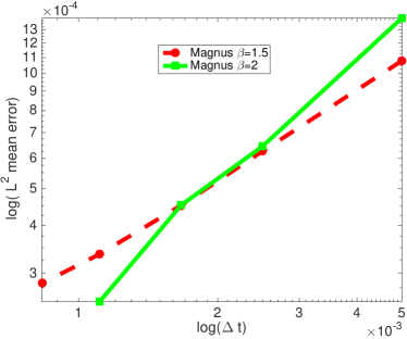
Figure 1. Convergence of the stochastic Magnus scheme for $\beta=1.5$ and $\beta=2$ in (152). The order of convergence in time is $0.995$ for $\beta=2$, and $0.7561$ for $\beta=1.5$. The total number of samples used is $100$.

In Figure 1, we can observe the convergence of the stochastic Magnus scheme for two noise’s parameters. Indeed the order of convergence in time is $0.995$ for $\beta=2$, and $0.7561$ for $\beta=1.5$. These orders are close to the theoretical orders $1$ and $0.75$ obtained in mainresult1 for $\beta=2$ and $\beta=1.5$ respectively.

References

• [1] H. Amann, On abstract parabolic fundamental solutions. J. Math. Soc. Jpn. 39(1987) 93-116
• [2] J. M. Clark and R. J. Cameron, The maximum rate of convergence of discrete approximations for stochastic differential equations. Stochastic Differential Systems (Proc. IFIP-WG 7/1 in Control and Information Science, Vol. 25 (1980). Berlin: Springer 162–171.
• [3] S. Blanes and P. C. Moan, Fourth- and sixth-order commutator-free Magnus integrators for linear and non-linear dynamical systems. Appl. Numer. Math. 56 (2006) 1519–1537.
• [4] F. Casas and A. Murua, An efficient algorithm for computing the Baker-Hausdorff series and some of its applications. J. Math. Phys. 50 (2009) 033513
• [5] P. L. Chow, Stochastic partial differential equations. Chapman & Hall/CRC. Appl. Math. Nonlinear Sci. ser., 2007.
• [6] C. M. Elliot and S. Larsson, Error estimates with smooth and nonsmooth data for a finite element method for the Cahn-Hilliard equation. Math. Comput. 58 (1992) 603–630.
• [7] L. C. Evans, Partial Differential Equations. Grad. Stud. Vol. 19 (1997)
• [8] H. Fujita and T. Suzuki, Evolutions problems (part1) in: P. G. Ciarlet and J. L. Lions(eds.), Handb. Numer. Anal., vol. II, North-Holland, pp. 789–928 (1991).
• [9] C. González, A. Ostermann and M. Thalhmmer, A second-order Magnus-type integrator for non autonomous parabolic problems. J. Comput. Appl. Math. 189 (2006) 142–156.
• [10] C. González and A. Ostermann, Optimal convergence results for Runge-Kutta discretizations of linear nonautonomous parabolic problems. BIT 39(1) (1999) 79-95.
• [11] D. Henry, Geometric Theory of semilinear parabolic equations. Lecture notes in Mathematics, vol. 840, Berlin : Springer, 1981.
• [12] D. Hipp, M. Hochbruck and A. Ostermann, An exponential integrator for non-autonomous parabolic problems. Elect. Trans. on Numer. Anal. 41 (2014) 497-511.
• [13] M. Hochbruck and C. Lubich, On Magnus integrators for time-dependent Schrödinger equations. SIAM. J. Numer. Anal. 41 (2003) 945-963.
• [14] A. Iserles, H. Z. Munthe-Kaas, S. P. Nørsett and A. Zanna, Lie group methods. Acta Numer. 9 (2000) 215-365.
• [15] A. Jentzen, P. E. Kloeden and G. Winkel, Efficient simulation of nonlinear parabolic SPDEs with additive noise. Ann. Appl. Probab. 21(3) (2011) 908-950.
• [16] A. Jentzen and M. Röckner, Regularity analysis for stochastic partial differential equations with nonlinear multiplicative trace class noise. J. Diff. Equat. 252 (2012) 114-136.
• [17] P. E. Kloeden, G. J. Lord, A. Neuenkirch and T. Shardlow, The exponential integrator scheme for stochastic partial differential equations: Pathwise error bounds. J. Comput. Appl. Math. 235 (2011) 1245-1260.
• [18] P. E. Kloeden and E. Platen, Numerical solutions of differential equations. Springer Verlag (1992)
• [19] R. Kruse, Optimal error estimates of Galerkin finite element methods for stochastic partial differential equations with multiplicative noise. IMA J. Numer., 34 (2014) 217-251.
• [20] R. Kruse ans S. Larsson, Optimal regularity for semilinear stochastic partial differential equations with multiplicative noise. Electron. J. Probab. 17(65) (2012) 1-19.
• [21] M. Kovács, S. Larsson and F. Lindgren, Strong convergence of the finite element method with truncated noise for semilinear parabolic stochastic equations with additive noise. Numer. Algor. 53 (2010) 309-220.
• [22] S. Larsson, Semilinear parabolic partial differential equations : theory, approximation, and application. In new Trends in the Mathematical and computer sciences, pp. 153-194. Cent. Math. Comp. Sci. (ICMCS), Lagos, 2006.
• [23] S. Larsson, Nonsmooth data error estimates with applications to the study of the long-time behavior of the finite elements solutions of semilinear parabolic problems. Preprint 6, Departement of Mathematics, Chalmers University of Technology (1992). Available at http://www.math.chalmers.se/∼stig/papers/index.html.
• [24] J. L. Lions, Espaces d´interpolation et domaines de puissances fractionnaires d´operateurs. Soc. Jpn. 14 (1962) 233-241.
• [25] G. J. Lord and A. Tambue, Stochastic exponential integrators for the finite element discretization of SPDEs for multiplicative and additive noise. IMA J. Numer. Anal. 33(2) (2013) 515-543.
• [26] G. J. Lord and A. Tambue, A modified semi-implict Euler-Maruyama scheme for finite element discretization of SPDEs with additive noise. Appl. Math. Comput. 332 (2018) 105-112.
• [27] Y. Y. Lu, A fourth-order Magnus scheme for Helmholtz equation. J. Compt. Appl. Math. 173 (2005) 247-253.
• [28] M. Magnus, On the exponential solution of a differential equation for a linear operator. Comm. Pure Appl. Math. 7 (1954) 649-673.
• [29] B. Mielnik and A. Murua, Combinatorial approach to Baker-Hausdorff exponents. Ann. Inst. Henri Poincaré A, 12(3) (1970) 215–254.
• [30] J. D. Mukam and A. Tambue, Strong convergence analysis of the stochastic exponential Rosenbrock scheme for the finite element discretization of semilinear SPDEs driven by multiplicative and additive noise. J. Sci. Comput. 74 (2018) 937-978.
• [31] T. Nambu, Characterization of the Domain of Fractional Powers of a Class of Elliptic Differential Operators with Feedback Boundary Conditions. J. Diff. Eq. 136 (1997) 294-324.
• [32] A. Pazy, Semigroup of Linear Operators and Applications to Partial Differential Equations. Springer, new York, 1983.
• [33] D. G. Prato, and J. Zabczyk, Stochastic equations in infinite dimensions. Encyclopedia of Mathematics and its Applications, vol. 44. Cambridge : Cambridge University press, 1992.
• [34] C. Prévôt and M. Röckner, A Concise Course on Stochastic Partial Differential Equations. Lecture Notes in Mathematics, vol. 1905, Springer, Berlin, 2007.
• [35] R. Seely, Norms and domains of the complex powers $A_{B^{z}}$. Amer. J. Math. 93 (1971) 299-309.
• [36] J. Seidler and Praha, Da Prato-Zabczyk’s maximal inequality revisited I. Math. Bohem. 118(1) (1993) 67-106.
• [37] D. Scholz and M. Weyrauch, A note on the Zassenhaus product formula. J. Math. Phys. 47(3) (2006) 033505.
• [38] A. Tambue and J. D. Mukam, Convergence analysis of the Magnus-Rosenbrock type method for the finite element discretization of semilinear non autonomous parabolic PDE with nonsmooth initial data. https://arxiv.org/abs/1809.03227,2018.
• [39] A. Tambue and J. D. Mukam, Magnus-type integrator for the finite element discretization of semilinear parabolic non autonomous SPDEs driven by multiplicative noise. https://arxiv.org/abs/1809.04438, 2018.
• [40] A. Tambue and J. M. T. Ngnotchouye, Weak convergence for a stochastic exponential integrator and finite element discretization of stochastic partial differential equation with multiplicative & additive noise. Appl. Numer. Math. 108 (2016) 57-86.
• [41] H. Tanabe, Equations of Evolutions. Pitman, London, 1979.
• [42] V. Thomée, Galerkin Finite Element Methods for Parabolic Problems, 2nd edn. Springer Series in Computational Mathematics, Vol. 25. Berlin: Springer, 2006.
• [43] X. Wang, Strong convergence rates of the linear implicit Euler method for the finite element discretization of SPDEs with additive noise. IMA J. Numer. Anal. 37 (2017) 965-984.
• [44] X. Wang and Q. Ruisheng, A note on an accelerated exponential Euler method for parabolic SPDEs with additive noise. Appl. Math. Lett. 46 (2015) 31-37.
• [45] X. Wang, An exponential integrator scheme for time discretization of nonlinear wave equation. J. Sci. Comput. 64 (2015) 234-263.
• [46] Y. Yan, Galerkin finite element methods for stochastic parabolic partial differential equations. SIAM J. Num. Anal., 43(4) (2005) 1363-1384.