Improving Reinforcement Learning Based Image Captioning with Natural Language Prior

Abstract

Recently, Reinforcement Learning (RL) approaches have demonstrated advanced performance in image captioning by directly optimizing the metric used for testing. However, this shaped reward introduces learning biases, which reduces the readability of generated text. In addition, the large sample space makes training unstable and slow. To alleviate these issues, we propose a simple coherent solution that constrains the action space using an $n$-gram language prior. Quantitative and qualitative evaluations on benchmarks show that RL with the simple add-on module performs favorably against its counterpart in terms of both readability and speed of convergence. Human evaluation results show that our model is more human readable and graceful. The implementation will become publicly available upon the acceptance of the paper.

1 Introduction

Image captioning Farhadi et al. (2010); Kulkarni et al. (2011); Yao et al. (2017); Lu et al. (2016); Dai et al. (2017); Li et al. (2017) aims at generating natural language descriptions of images. Advanced by recent developments of deep learning, many captioning models rely on an encoder-decoder based paradigm Vinyals et al. (2015), where the input image is encoded into hidden representations using a Convolutional Neural Network (CNN) followed by a Recurrent Neural Network (RNN) decoder to generate a word sequence as the caption. Further, the decoder RNN can be equipped with spatial attention mechanisms Xu et al. (2015) to incorporate precise visual contexts, which often yields performance improvements empirically.

Although the encoder-decoder framework can be effectively trained with maximum likelihood estimation (MLE) Salakhutdinov (2010), recent research Ranzato et al. (2015) have pointed out that the MLE based approaches suffer from the so-called exposure bias problem. To address this problem, Ranzato et al. (2015) proposed a Reinforcement Learning (RL) based training framework. The method, developed on top of the REINFORCE algorithm Williams (1992), directly optimizes the non-differentiable test metric (e.g. BLEU Papineni et al. (2002), CIDEr Vedantam et al. (2015), METEOR Banerjee and Lavie (2005) etc.), and achieves promising improvements. However, learning with RL is a notoriously difficult task due to the high-variance of gradient estimation. Actor-critic Sutton and Barto (1998) methods are often adopted, which involves training an additional value network to predict the expected reward. On the other hand, Rennie et al. (2017) designed a self-critical method that utilizes the output of its own test-time inference algorithm as the baseline to normalize the rewards, which leads to further performance gains.

Beside to the high-variance problem, we notice that there are two other drawbacks of RL-based captioning methods that are often overlooked in the literature. First, while these methods can directly optimize the non-differentiable rewards and achieve high test scores, the generated captions contain many repeated trivial patterns, especially at the end of the sequence. Table 1 shows examples of bad-endings generated by a self-critical based RL algorithm (model details refer to Section 4). Specifically, 46.44% generated captions end with phrases as “with a”, “on a”, “of a”, etc. (for detailed statistics see Appendix A), on the MSCOCO Chen et al. (2015) validation set with the standard data splitting by Karpathy and Li (2015). The reason is that the shaped reward function biases the learning. In Figure 1, we see these additive patterns at the end of captions, although make no sense to humans, yield to a higher reward. Empirically, removing these endings results in a huge performance drop of around 6%. Paulus et al. (2017) has also reported that in abstractive summarization, using RL only achieves high ROUGE Lin (2004) score, yet the human-readability is very poor. The second drawback is that RL-based text generation is sample-inefficient due to the large action space. Specifically, the search space is of size $O(|\mathcal{V}|^{T})$, where $\mathcal{V}$ is a set of words, $T$ is the sentence length, and $|\cdot|$ denotes the cardinality of a set. This often makes training unstable and converge slowly.

In this work, to tackle these two issues, we propose a simple yet effective solution by introducing coherent language constraints on local action selections in RL. Specifically, we first obtain word-level $n$-gram Kneser and Ney (1995) model from the training set and then use it as an effective prior. During the action sampling step in RL, we reduce the search space of actions based on the constitution of the previous word contexts as well as our $n$-gram model. To further promote samples with high rewards, we sample multiple sentences during the training and update the policy based on the best-rewarded one. Such simple treatments prevent the appearance of bad endings and expedite the convergence while maintaining comparable performance to the pure RL counterpart. In addition, the proposed framework is generic, which can be applied to many different kinds of neural structures and applications.

Image ID	Generated sentence	CIDEr
262262	a tall building with a clock tower with a	160.1
262148	a man doing a trick on a skateboard on a	146.5
52413	a person holding a cell phone in a	132.4
393225	a bow of soup with carrots and a	118.5

Table 1: Examples of bad sequences generated by a self-critical based RL baseline. Blue color indicates the bad ending. Sequences with bad endings have high CIDEr scores.

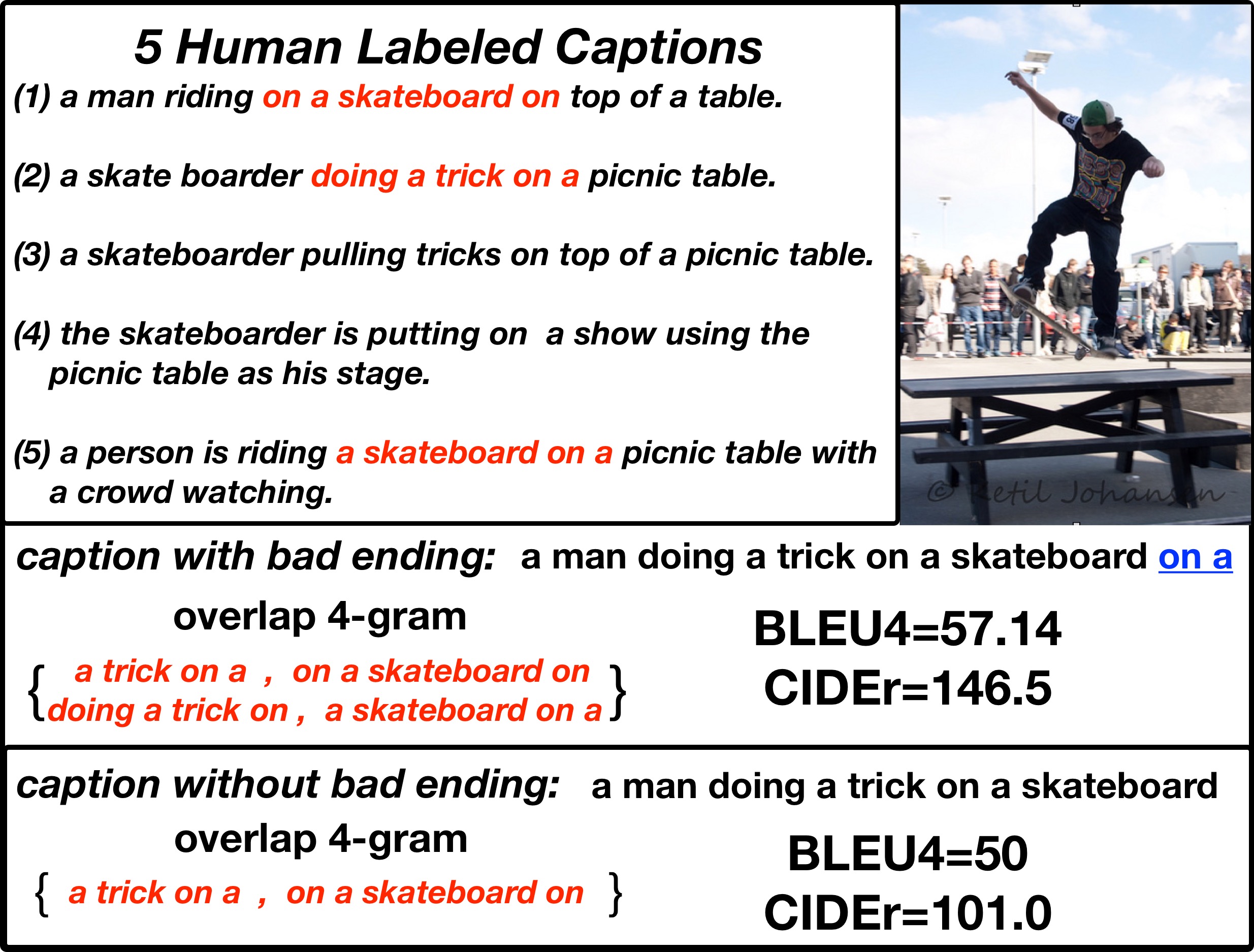
Figure 1: A demonstration of the sequence with bad ending has higher BLEU and CIDEr scores compared to the one without.

2 Model Architecture

Encoder-Decoder Model:

We adopt a similar structure as GNIC Vinyals et al. (2015), which first encodes an image $I$ to a dense vector $h_{I}$ by CNN. The vector $h_{I}$ is then fed as the input to an LSTM-based Hochreiter and Schmidhuber (1997) language model decoder. At each step $t$, the LSTM receives the previous output $w_{t-1}$ as the input; computes the hidden state $h_{t}$; and predicts the next word $w_{t}$ as below:

$$h_{t}=\text{LSTM}(h_{t-1},w_{t-1}),~{}~{}l_{t}=W_{l}h_{t}$$ (1)

$$w_{t}\sim\text{softmax}(l_{t}),$$

where $w_{0}=h_{I}$ and $h_{0}$ and $c_{0}$ are initialized to zero. The generation ends if a special token *end* is predicted.

Attention Model:

Instead of utilizing a static representation of the image, attention mechanism dynamically reweights the spatial features from CNN to focus on the different region of the image at each word generation. We specifically consider the standard architecture used in Xu et al. (2015), where $\mathcal{A}=\{a_{1},a_{2},...,a_{L}\}$ is the spatial feature set and each $a_{i}\in R^{D}$ corresponds to features extracted at different image locations. Then the hidden states of the LSTM is computed as

$$e_{ti}=f_{\text{att}}(a_{i},h_{t-1}),~{}~{}\beta_{ti}=\frac{\text{exp}(e_{ti})}{\sum_{k=1}^{L}\text{exp}(e_{tk})},$$ (2)

$$z_{t}=\sum_{k=1}^{L}\beta_{tk}a_{k},~{}~{}h_{t}=\text{LSTM}([h_{t-1},z_{t}],w_{t-1}),$$

where $f_{\text{att}}$ is an attention model, which we use a single fully connected layer conditioned on the previous hidden state. Once $h_{t}$ is obtained, the word generation is same as equation (1).

Sequence Generation with RL:

We follow the training procedure of Rennie et al. (2017). The decoder LSTM can be viewed as a “policy” denoted by $p_{\theta}$, where $\theta$ is the set of parameters of the network. At each time step $t$, the policy chooses an action by generating a word $w_{t}$ and obtains a new “state” (i.e. hidden states of LSTM, attention weights, etc.). Once the end token is generated, a “reward” $r$ is given based on the score (e.g. CIDEr or BLEU) of the predicted sentence. The goal is to maximize the expected reward as

$$L(\theta)=\mathbb{E}_{w^{s}\sim p_{\theta}}[r(w^{s})],$$ (3)

where $w^{s}=\{w^{s}_{1},w^{s}_{2},...,w^{s}_{T}\}$ are sampled words at every time step. The REINFORCE algorithm Williams (1992) provides unbiased gradient estimation of $\theta$ as

$$\nabla_{\theta}{L}(\theta)\approx r(w^{s})\nabla_{\theta}{\log{p_{\theta}(w^{s})}},$$ (4)

using a single sequence.

Variance Reduction with Self-Critical:

We reduce the variance of the gradient estimator by using the self-critical approach as

$$\nabla_{\theta}{L}(\theta)\approx(r(w^{s})-r(\bar{w}))\nabla_{\theta}{\log{p_{\theta}(w^{s})}},$$ (5)

where $\bar{w}_{t}$ is the baseline reward calculated by the current model under the inference algorithm used at test time defined as

$$\bar{w}_{t}=\mathop{\arg\max}_{w_{t}}p_{\theta}(w_{t}|h_{t}).$$ (6)

Then, sequences have rewards higher than $\bar{w}$ will be increased in probability, while samples result in lower reward will be suppressed.

3 Prior Language Constraint with $N$-Gram Model

Method:

We collect all $n$-grams ($n$=3 or 4 in our experiments) from a corpus of captions. We use the training set from MSCOCO to avoid the usage of the additional resource. Thus, a fair comparison to previous methods is guaranteed. Then, we filter the $n$-grams with frequencies lower than five. The set of remaining ones is denoted as $\mathcal{F}$. During training, given the previous tokens predicted by the decoder, we constraint the sample space the current prediction by

$$\vspace{-0.05in}w_{t}\sim\text{softmax}(p_{\theta}(w^{s}_{t})\cdot\boldsymbol{\alpha_{t}}),$$ (7)

where $\boldsymbol{\alpha_{i}}$ is an indicator vector whose length is the vocabulary size $|\mathcal{V}|$ and its elements are non-zero only if the corresponding word and the previous ($n-1$)-gram constitute a valid $n$-gram in $\mathcal{F}$ as

$$\boldsymbol{\alpha_{t}}[k]= \begin{cases}1&\mbox{if $\{w^{s}_{t-n+1},\cdots,w^{s}_{t-1},k\}\in\mathcal{F}$}\\ 0&\mbox{otherwise}\end{cases}.$$ (8)

	Methods	CIDEr	BLEU4	ROUGE-L	METEOR	BadEnd-Rate
Published	Karpathy and Li (2015)	66.0	23.0	- -	19.5	0.0
	Xu et al. (2015)	- -	25.0	- -	23.0	0.0
	MIXER Ranzato et al. (2015)	- -	29.1	- -	- -	- -
	Ren et al. (2017)	93.7	30.4	52.5	25.1	- -
Implemented	ED-XE	89.8	28.0	51.7	24.2	0.0
	Att-XE	95.1	29.2	52.8	24.8	0.0
	ED-SC Rennie et al. (2017)	101.8 / 96.1	31.2 / 30.3	53.1 / 52.9	24.6 / 23.9	46.4% / 0.0
	Att-SC Rennie et al. (2017)	105.7 / 100.8	32.3 / 30.8	53.8 / 53.1	25.2 / 24.1	43.7% / 0.0
	Ours-ED-4-gram	96.7	29.1	51.4	23.9	0.0
	Ours-Att-4-gram	102.0	30.2	53.6	25.6	0.0
	Ours-ED-tri-gram	95.1	29.8	52.4	24.1	0.0
	Ours-Att-tri-gram	100.4	28.7	51.8	25.0	0.0

Table 2: Quantitative evaluation of our method compared to baselines on MSCOCO. Blue text indicates the performance after adjustments and red text indicates the best performance.

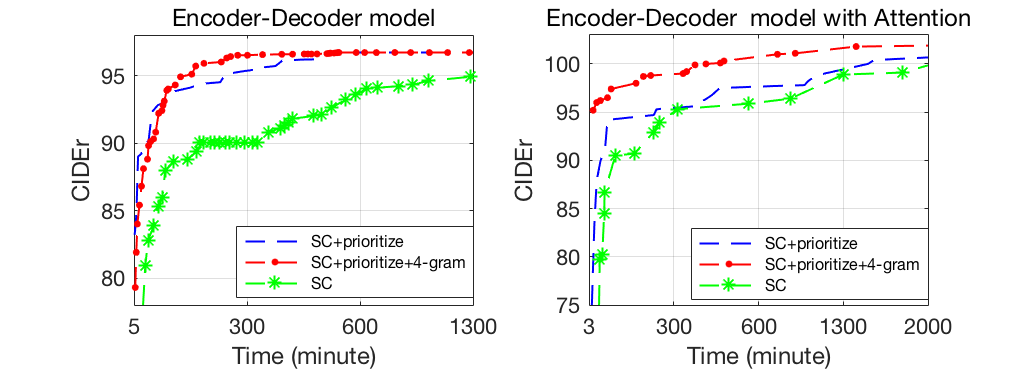
Figure 2: Training time of models with (right) and without (left) spatial attention.

Discussion:

The key motivation for applying the above constraint is two-fold: (1) this ensures generated captions always formed by valid $n$-grams, which provides us a direct way of eliminating the repeated common phrases and bad-endings like the ones in Table 1; and (2) this shrinks the size of action space, which makes the training converges much faster. For MSCOCO, action space is changed from more than 9,000 to 56 on average.

4 Experiments

Dataset:

We perform both quantitative and qualitative evaluations on MSCOCO dataset. The dataset contains 123,287 images and each image has at least five human captions. To seek fair comparison to others, we use the publicly available splits, which contains 82,783 training, 5,000 validation and 5,000 testing images.

Implementation Details:

Our implementations are based on the publicly project. We use an ImageNet pre-trained 101-layered ResNet He et al. (2016) to extract visual features. We consider two types (see Section 2) of architectural training with RL: (1) the plain encoder-decoder, and (2) the encoder-decoder with attention. For the former one, we represent each image by a 2,048-dimension vector by extracting the features from the last convolutional layer with average pooling. For the attention model, we apply spatial adaptive max pooling and the output feature map has the size of $14\times 14\times 2,048$. At each time step, the attention model produces weights over 196 spatial locations. The size of word embeddings and the hidden dimension of the LSTM are set to 512 for all experiments. More details are in Appendix B.

Compared Methods:

We report our results in four different settings, which include the combinations of with/without attention and using tri-/four-gram. We directly compare with our counterparts that have the same structures but no $n$-gram modules. Specifically, they are encoder-decoder based self-critical (ED-SC), and the one with attention (Att-SC). In addition, since our experimental setup is almost identical to many existing works, we also include their reported results, which include Karpathy and Li (2015); Xu et al. (2015); Ranzato et al. (2015); Ren et al. (2017). At last, we also include the performance of our warm-start models - the models trained by MLE Vinyals et al. (2015) using cross entropy (ED-XE and Att-XE) - as a reference.

Evaluation Metric and Performance Adjustment:

We report performance on FIVE metrics: BLEU4, METEOR, ROUGE-L,CIDEr and Bad Ending Rate. For the self-critical baselines, we report two sets of performances: 1) the captions directly generated by the model; and 2) the sequences of removing bad endings of the generated captions, based on the distribution in Appendix A.

Results:

Table 2 summarizes the performances of our models compared with other baselines. We see that without performance adjustments, the self-critical RL with attention performs the best. However, since it contains many bad endings, our method achieves supreme results after these repeated patterns are removed. We also provide some qualitative comparison between our attention model and self-critical in Appendix C.

Efficient Training:

We show that constraining the action space leads to a more efficient RL training in Figure 2. CIDEr score is calculated after removing bad endings. We plot three curves using architectures with/without attentions. The Green curve is the self-critical, the blue one is with prioritized sampling, and the red one is our final model with 4-gram constraint. We observe that we can speed up almost twice than its counterpart.

Online Evaluation:

We also evaluate our attention model on COCO online server and results are reported in Table 3. Att-SC gets a higher score than ours in the online test, however, with a lot of bad endings where the bad ending ratio is 72.7$\%$.

Methods	CIDEr	BLEU4	METEOR	ROUGE-L	BadEnd-Rate
Att-SC	109.3	61.9	32.9	67.7	72.7%
Att-4-gram	104.7	59.8	33.0	66.2	0
Att-LSTM-LM	104.3	61.0	33.9	68.5	0

Table 3: Quantitative results on online server (C40 test).Red text indicates the best performance.

Methods	CIDEr	BLEU4	ROUGE-L	METEOR	BadEnd-Rate
Att-SC Rennie et al. (2017)	105.7 / 100.8	32.3 / 30.8	53.8 / 53.1	25.2 / 24.1	43.7% / 0.0
Ours-ED-4-gram	96.7	29.1	51.4	23.9	0.0
Ours-Att-4-gram	102.0	30.2	53.6	25.6	0.0
ED-LSTM-LM	99.4	30.9	52.7	24.6	0.0
Att-LSTM-LM	105.9	32.8	54.1	25.4	0.0

Table 4: Quantitative evaluation with our extension methods on MSCOCO. Blue text indicates the performance after adjustments and red text indicates the best performance.

Human Evaluation:

We also implement human evaluation on the results generated by our Att-4-gram compared with Att-SC. We randomly select 200 images from the test set. Each time, one image with two captions generated by two different models are shown to the volunteer and three choices are provided: (1) the first one is better; (2) both are the same level; (3) the second one is better. See more details in Appendix D. In Table 5, our model wins 400 times and performs more closely to human than Att-SC.

Methods	4-gram win	Same level	4-gram lose
4-gram VS SC	400	349	251

Table 5: Human evaluation results for attention models

Evaluating Captions Diversity:

To further evaluate the quality of the caption model, we follow Shetty et al. (2017) to measure the diversity of the generated captions. We compute the novelty score of our 4-gram model, which is defined as whether a particular caption has been observed in the training set. When two models have the same level predictive performances (e.g. CIDEr), a higher novelty score usually indicates more diverse generations. We conduct the experiment five times and report the averaged novelty score of our 4-gram model and the Att-SC, which are 77.83% and 59.28% respectively. As the reference, the METEOR and novelty scores reported in Shetty et al. (2017) are 23.6, and 79.84%, respectively.

5 Neural Language Models Extension

Inspired by the paper reviews, we extend our model by adopting another language prior to evaluating the effectiveness of constraining action space during REINFORCE training. We train our neural language model based on the MSCOCO caption corpus with an LSTM unit.

LSTM Language Model:

Given a word series $\{w_{0},w_{1},...,w_{T}\}$, the target of a neural language model is to maximize the log-likelihood as:

$$\mathop{\max}_{\theta}\log p_{\theta}(w_{0},w_{1},...,w_{T}).$$ (9)

We model $p_{\theta}(w_{0},w_{1},...,w_{T})$ by an LSTM unit:

$$\log p_{\theta}( w_{0},...,w_{T})=\sum_{t=1}^{T}\log p_{\theta_{LM}}(w_{t}|h_{t-1})$$ (10)

$$h_{t}=\text{LSTM}_{LM}(h_{t-1},w_{t-1}),$$

where $w_{0}$ is set to a *start* token for all sentences. $h_{0}$ and $c_{0}$ are initialized to zero. After obtaining the optimized $\theta^{*}_{LM}$, we can use it to constrain the action space similar to the N-gram language model. Specifically, given previous $t-1$ sampled words from current caption model, we compute $p_{\theta^{*}_{LM}}(w_{t}|w_{0},w_{1},...,w_{t-1})$, which is the probability of the next word over the entire vocabulary. We then apply a simple thresholding rule to form a subset of valid words for the captioning model.

$$\boldsymbol{\alpha_{t}}[k]=\begin{cases}1&\mbox{if $\{k\}\in\mathcal{F}$}\\ 0&\mbox{otherwise}\end{cases},\text{where}$$ (11)

$$\mathcal{F}= \{w_{t}|p_{\theta^{*}_{LM}}(w_{t}|w_{0},w_{1},...,w_{t-1})\geq\eta\}.$$

$\eta$ is a hyperparameter.

Additional Experiments

The word embedding size and hidden dimension of $\theta_{LM}$ are set to 256 for this experiment. We use Adam optimizer for training language model and the learning rate is set to 0.001. The batch size of language model training and REINFORCE training are both set to 20 in the experiments. $\eta$ is set to 0.00005 for the first word and increases by a factor of two for every timestep. We report our results in two settings, which include the combination of with/without attention for the caption model (termed ED-LSTM-LM and Att-LSTM-LM). We use the same warm-start models as in the N-gram experiments. The performances are summarized in Table 4 and Table 3. We see that the neural language model provides further performance gains compared to the N-gram model without introducing any bad-endings. This is because that the LSTM language model covers a larger context than N-gram, which helps to generate more accurate captions.

6 Conclusion

In this paper, we present a simple but efficient approach to RL-based image caption by considering $n$-gram language prior to constrain the action space. Our method converges faster and achieves better results than self-critical setting after removing bad endings in the generated captions. In addition, captions generated by our models are more human readable and graceful. We further extend our ideas using neural language model. The results demonstrate that the captioning models are more beneficial from the neural language model than the N-gram model.

Appendix A Statistics of Bad Endings

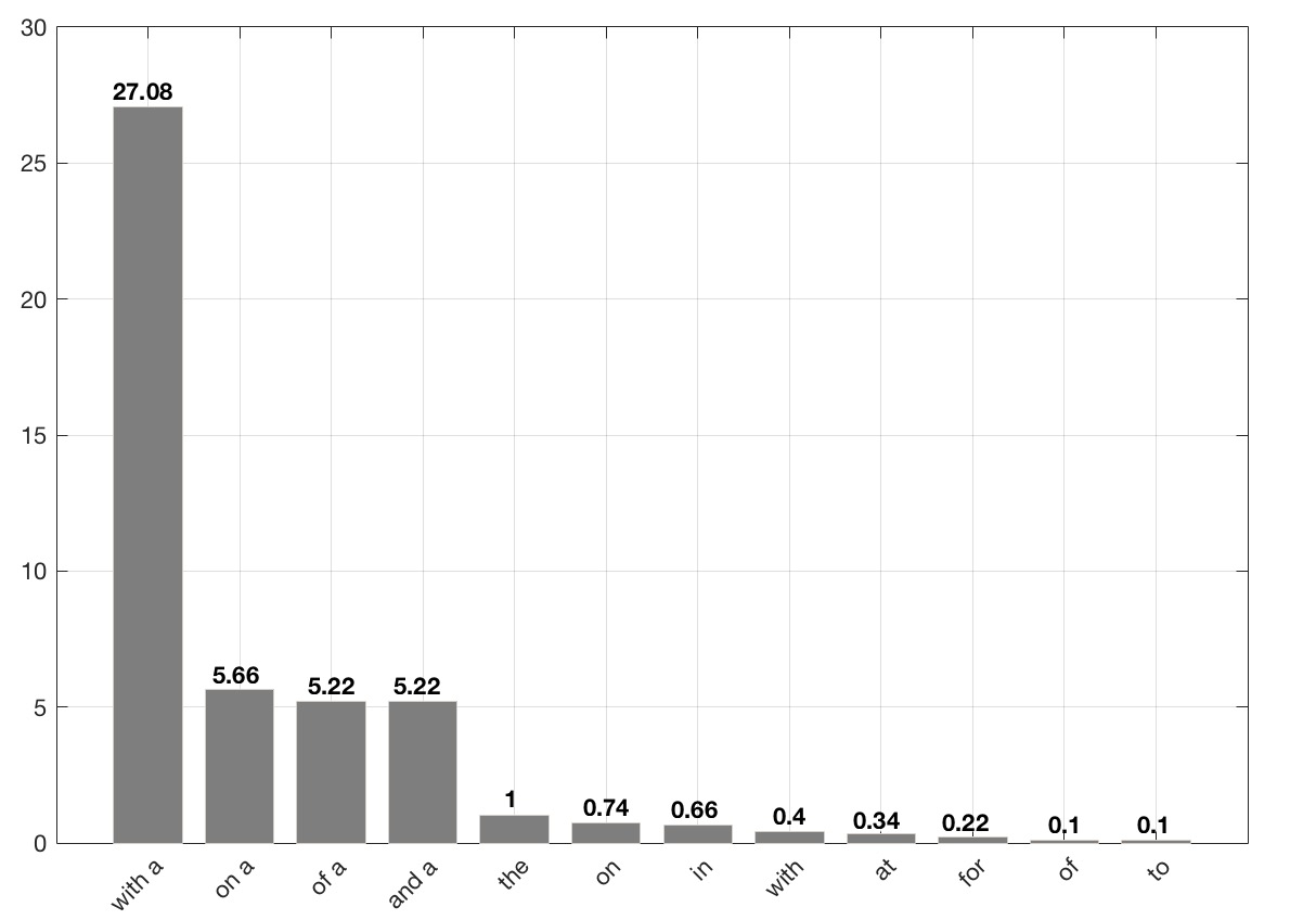
Figure 3: Statistics of bad endings over 5,000 validation instances generated by self-critical method optimized on the CIDEr metric.

Appendix B More training details

We drop any words that have appeared less than five times. The vocabulary size is 9,488. We do not rescale or crop the images when extracting CNN features for the attention model. At the beginning of RL training, the learning rate is $5\times 10^{-5}$ and we anneal it by a factor of 0.2 when the CIDEr score on validation set has no improvement for over 10 epochs. The CNN weights are fixed during our RL training process. We use a Gumbel sampler and perform our action sampling on GPU devices which is much faster than CPU device. The batch size is set to 50 in all our experiments. In our observation, we discover that a very powerful warm-start model is necessary to maintain the stability and convergence speed of self-critical without our prioritized sampling and n-gram constraints while our methods need not.

We warm-start all models by training them under the cross-entropy objective. We use ADAM Kingma and Ba (2015) optimizer with an initial learning rate of $5\times 10^{-4}$. We select the model with best CIDEr scores on the development set to initialize RL training and use a Gumbel sampler Kusner and Hernándezlobato (2016) to improve action sampling efficiency. In order to promote captions with higher reward, we sample multiple sequences (we set 10 in our experiments) during the training and update the parameters based on the sample with the highest rewards. We find that this technique empirically helps convergence.

Appendix C Qualitative Comparison

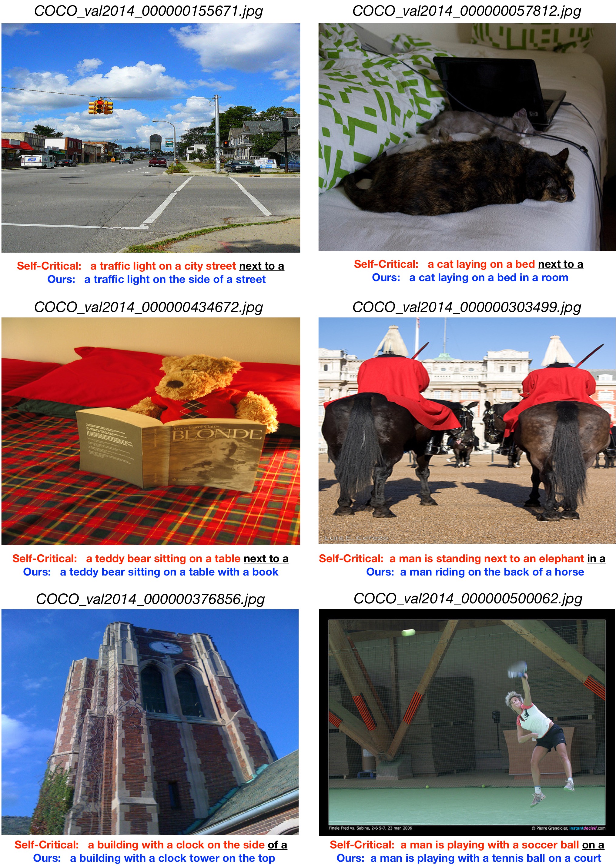
Figure 4: Examples generated by our model with attention compared to the self-critical counterpart. After adding N-gram constraints, our results are more accurate and human-readable.

Appendix D Human Evaluation Details

We recruit 10 volunteers who are under the correct guidance for finishing the human evaluation process.We implement our human evaluation experiment on a web page (see Figure 5).

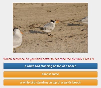
Figure 5: Web page for human evaluation

Every time the volunteer must make a choice among these three choices. And ”almost same” means that two captions are both good or both bad for the given images. Each image must be evaluated by at least 5 volunteers.

The order of caption generated from given model is random so the volunteers have no idea where these captions come from which model. Some times the first one comes from Ours-Att-4-gram, and some times from Att-SC.

References

- Banerjee and Lavie (2005) Satanjeev Banerjee and Alon Lavie. 2005. Meteor: An automatic metric for mt evaluation with improved correlation with human judgments. In ACL-workshop, pages 228–231.
- Chen et al. (2015) Xinlei Chen, Hao Fang, Tsung Yi Lin, Ramakrishna Vedantam, Saurabh Gupta, Piotr Dollar, and C. Lawrence Zitnick. 2015. Microsoft coco captions: Data collection and evaluation server. Computer Science.
- Dai et al. (2017) Bo Dai, Sanja Fidler, Raquel Urtasun, and Dahua Lin. 2017. Towards diverse and natural image descriptions via a conditional gan. In ICCV, pages 2989–2998.
- Farhadi et al. (2010) Ali Farhadi, Mohsen Hejrati, Mohammad Amin Sadeghi, Peter Young, Cyrus Rashtchian, Julia Hockenmaier, and David Forsyth. 2010. Every picture tells a story: generating sentences from images. Lecture Notes in Computer Science, 21(10):15–29.
- He et al. (2016) Kaiming He, Xiangyu Zhang, Shaoqing Ren, and Jian Sun. 2016. Deep residual learning for image recognition. In CVPR, pages 770–778.
- Hochreiter and Schmidhuber (1997) Sepp Hochreiter and Jürgen Schmidhuber. 1997. Long short-term memory. Neural Computation, 9(8):1735–1780.
- Karpathy and Li (2015) Andrej Karpathy and Fei Fei Li. 2015. Deep visual-semantic alignments for generating image descriptions. In CVPR, pages 3128–3137.
- Kingma and Ba (2015) Diederik Kingma and Jimmy Ba. 2015. Adam: A method for stochastic optimization. In ICLR.
- Kneser and Ney (1995) Reinhard Kneser and Hermann Ney. 1995. Improved backing-off for m-gram language modeling. In Acoustics, Speech, and Signal Processing, 1995. ICASSP-95., 1995 International Conference on, volume 1, pages 181–184. IEEE.
- Kulkarni et al. (2011) G. Kulkarni, V. Premraj, S. Dhar, Siming Li, Yejin Choi, A. C. Berg, and T. L. Berg. 2011. Baby talk: Understanding and generating simple image descriptions. In CVPR, pages 1601–1608.
- Kusner and Hernándezlobato (2016) Matt J. Kusner and José Miguel Hernándezlobato. 2016. Gans for sequences of discrete elements with the gumbel-softmax distribution.
- Li et al. (2017) Yikang Li, Wanli Ouyang, Bolei Zhou, Kun Wang, and Xiaogang Wang. 2017. Scene graph generation from objects, phrases and region captions. In ICCV, pages 1270–1279.
- Lin (2004) Chin-Yew Lin. 2004. Rouge: A package for automatic evaluation of summaries. In ACL-workshop, page 10.
- Lu et al. (2016) Jiasen Lu, Caiming Xiong, Devi Parikh, and Richard Socher. 2016. Knowing when to look: Adaptive attention via a visual sentinel for image captioning. pages 3242–3250.
- Papineni et al. (2002) Kishore Papineni, Salim Roukos, Todd Ward, and Wei-Jing Zhu. 2002. Bleu: a method for automatic evaluation of machine translation. In ACL, pages 311–318.
- Paulus et al. (2017) Romain Paulus, Caiming Xiong, and Richard Socher. 2017. A deep reinforced model for abstractive summarization. arXiv preprint arXiv:1705.04304.
- Ranzato et al. (2015) Marc’Aurelio Ranzato, Sumit Chopra, Michael Auli, and Wojciech Zaremba. 2015. Sequence level training with recurrent neural networks. Computer Science.
- Ren et al. (2017) Zhou Ren, Xiaoyu Wang, Ning Zhang, Xutao Lv, and LiJia Li. 2017. Deep reinforcement learning-based image captioning with embedding reward. In CVPR, pages 1151–1159.
- Rennie et al. (2017) Steven J Rennie, Etienne Marcheret, Youssef Mroueh, Jarret Ross, and Vaibhava Goel. 2017. Self-critical sequence training for image captioning. In CVPR, pages 1179–1195.
- Salakhutdinov (2010) Ruslan Salakhutdinov. 2010. Learning deep generative models. 2(1):361–385.
- Shetty et al. (2017) Rakshith Shetty, Marcus Rohrbach, Lisa Anne Hendricks, Mario Fritz, and Bernt Schiele. 2017. Speaking the same language: Matching machine to human captions by adversarial training. In ICCV, pages 4155–4164.
- Sutton and Barto (1998) Richard S Sutton and Andrew G Barto. 1998. Reinforcement learning: An introduction, volume 1. MIT press Cambridge.
- Vedantam et al. (2015) Ramakrishna Vedantam, C Lawrence Zitnick, and Devi Parikh. 2015. Cider: Consensus-based image description evaluation. In CVPR, pages 4566–4575.
- Vinyals et al. (2015) Oriol Vinyals, Alexander Toshev, Samy Bengio, and Dumitru Erhan. 2015. Show and tell: A neural image caption generator. In CVPR, pages 3156–3164.
- Williams (1992) Ronald J Williams. 1992. Simple statistical gradient-following algorithms for connectionist reinforcement learning. In Reinforcement Learning, pages 5–32. Springer.
- Xu et al. (2015) Kelvin Xu, Jimmy Ba, Ryan Kiros, Aaron Courville, Ruslan Salakhutdinov, Richard Zemel, and Yoshua Bengio. 2015. Show, attend and tell: Neural image caption generation with visual attention. In ICML, pages 2048–2057.
- Yao et al. (2017) Ting Yao, Yingwei Pan, Yehao Li, Zhaofan Qiu, and Tao Mei. 2017. Boosting image captioning with attributes. In ICCV, pages 4904–4912.