Ensemble learning with 3D convolutional neural networks for functional connectome-based prediction

Abstract

The specificty and sensitivity of resting state functional MRI (rs-fMRI) measurements depend on preprocessing choices, such as the parcellation scheme used to define regions of interest (ROIs). In this study, we critically evaluate the effect of brain parcellations on machine learning models applied to rs-fMRI data. Our experiments reveal an intriguing trend: On average, models with stochastic parcellations consistently perform as well as models with widely used atlases at the same spatial scale. We thus propose an ensemble learning strategy to combine the predictions from models trained on connectivity data extracted using different (e.g., stochastic) parcellations. We further present an implementation of our ensemble learning strategy with a novel 3D Convolutional Neural Network (CNN) approach. The proposed CNN approach takes advantage of the full-resolution 3D spatial structure of rs-fMRI data and fits non-linear predictive models. Our ensemble CNN framework overcomes the limitations of traditional machine learning models for connectomes that often rely on region-based summary statistics and/or linear models. We showcase our approach on a classification (autism patients versus healthy controls) and a regression problem (prediction of subject’s age), and report promising results.

1 Introduction

Functional connectivity, as often captured by correlations in resting state functional MRI (rs-fMRI) data, has produced novel insights linking differences in brain organization to individual or group-level characteristics. Recently, machine learning models are being increasingly applied to study and exploit individual variation in functional connectivity data [1, 2, 3]. These models often employ hand-engineered features, such as pairwise correlations between regions of interest (ROIs) and network topological measures of clustering, modularity, small-worldness, integration, or segregation [4, 5, 6]. The ROIs are usually computed based on a pre-defined atlas or a parcellation scheme. The choice of the ROIs can have a significant impact on downstream analyses [7, 8, 9].

Brain ROIs can be defined based on macro-anatomical features, cytoarchitecture, functional activations, and/or connectivity patterns [10, 11, 12, 13]. A common approach is to derive the ROIs either based on input from experts and/or using a data-driven strategy on a small number of subjects. Expert-defined ROIs are challenging to standardize across studies [14] and often rely on arbitrary decisions. Data-driven ROIs, on the other hand, can be biased by the selection of the subjects, especially for regions that exhibit large variability across the population. Popular data-driven techniques include clustering, dictionary learning and Independent Component Analysis (ICA) [15, 16, 9]. Such methods can be sensitive to confounds such as motion, while initialization, optimization, and other algorithmic choices can also significantly influence the results [17]. A parcellation scheme not only defines the boundaries of ROIs, but also restricts the analysis to a certain spatial scale. Abraham et al. [18] showed that among various preprocessing decisions, the choice of region definition has the greatest impact on predictive accuracy with data-driven extraction based on dictionary learning outperforming ICA/clustering and other reference atlases.

Given the arbitrary nature of a chosen parcellation scheme and its impact on predictive models, we hypothesized that machine learning models can benefit markedly from an ensemble strategy that integrates across different scales and ROI definitions. Figure 1 shows a general schematic of our proposed framework. In this work, we conducted a thorough empirical evaluation of different choices for brain parcellations.

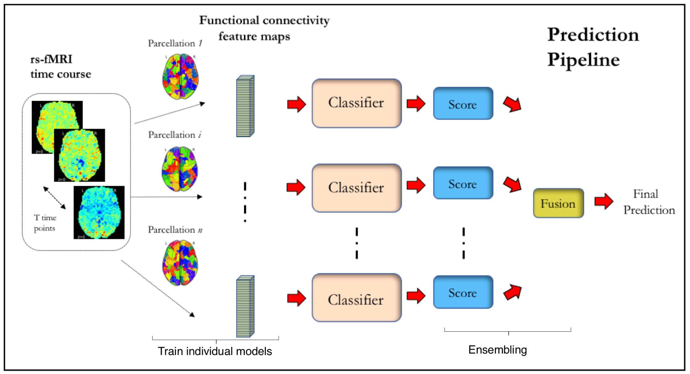
Figure 1: A general illustration of the proposed approach

Another important factor in connectome-based machine learning pertains to the choice of the classification algorithm. A large body of related work in the literature has focused on simple linear predictive models using vectorized connectivity data. A relatively recent trend is to exploit neural networks for graph-structured data, such as Graph Convolution Networks or BrainNet-CNN, to make individual-level predictions on connectomes. Ktena et al. [19] applied spectral graph convolutions in a distance-metric learning framework to train a k-nearest neighbor classifier on connectivity data. In a similar vein, Kawahara et al. [20] proposed the BrainNetCNN architecture that extends convolutional neural networks (CNNs) to handle graph-structured data. CNNs are motivated via the translation-invariance property of image-based classification problems and can exploit voxel/pixel resolution data. On the other hand, BrainNetCNN works directly with an adjacency matrix derived from the connectome data, while disregarding spatial information. The model parameter count would scale according to the number of ROIs, making the utilization of voxel-level connectivity infeasible with this approach. As we discuss below, we propose an alternative representation of connectivity data, which allows us to leverage modern deep learning architectures, like CNNs, to build a prediction model that exploits the full-resolution 3D spatial structure of rs-fMRI without having to learn too many model parameters.

In this work, we consider two applications: discrimination of autism patients and healthy controls; and regression of age. The first problem is a particularly challenging one. Several previous studies have reported altered functional connectivity patterns in Autism Spectrum Disorder (ASD) patients [21, 22, 23, 24]. While studies using small samples have reported classification accuracies over 75% [25], application of similar models on large heterogeneous datasets, such as ABIDE [26], have shown more modest performance levels over a wide range of connectome preprocessing schemes (accuracies that range 60-67%) [18].

Our main contributions in this paper are:

• An extensive evaluation of the influence of brain parcellations on functional connectome-based machine learning models

• An ensemble learning strategy for combining predictions from multiple classifiers corresponding to different brain parcellations

• An easy-to-implement 3D CNN framework for connectome-based classification

2 Materials and Methods

2.1 Dataset

The Autism Brain Imaging Data Exchange (ABIDE) is a multi-site consortium aggregating and openly sharing anatomical, functional MRI and phenotypic datasets of individuals diagnosed with ASD, as well as healthy controls (HC) [26]. The first phase of ABIDE (ABIDE-I) collected data from 1,112 individuals, comprising 539 individuals diagnosed with ASD and 573 typical controls across 17 sites. The second phase (ABIDE-II) aggregated 1,114 additional datasets, comprising 521 individuals with ASD and 593 healthy controls across 19 sites.

2.2 Preprocessing of fMRI Data

The Preprocessed Connectomes Project (PCP) released preprocessed versions of ABIDE-I using several pipelines [27]. We used the data processed through the Configurable Pipeline for the Analysis of Connectomes (CPAC). This pipeline performs motion correction, global mean intensity normalization and standardization of functional data to MNI space (3x3x3 mm resolution) before the extraction of ROI time series. Among the different strategies in the release, our analysis used data de-noised by regression of nuisance signals including motion parameters, CompCor WM+CSF components, and global signal, followed by band-pass filtering (0.01-0.1Hz). We note that we have experimented with alternate preprocessing strategies that include/exclude the global signal regression and CompCor steps. These results are presented in the Supplementary Section 7.6.

We preprocessed the ABIDE-II dataset following the same sequence of steps listed for ABIDE-I in CPAC (using the version v1.0.2a). Since manual quality control (QC) was not yet available for ABIDE-II, we performed an automatic QC by selecting those subjects that retained at least 100 frames or 4 minutes of fMRI scans after motion scrubbing [28]. Motion scrubbing was performed based on Framewise Displacement (FD), discarding one volume before and two volumes after the frame with FD exceeding 0.5mm [29].

2.3 Cohort selection

In our experiments, we used ABIDE-I subject data that passed manual QC by all the functional raters. This yielded a final sample size of 774 ABIDE-I subjects, comprising 379 subjects with ASD and 395 typical controls. As an independent test dataset, we employed ABIDE-II subjects from sites that participated in ABIDE-I and used the same MRI sequence parameters for data collection. After automatic QC, we ended up with a final ABIDE-II sample size of 163 individuals with ASD and 230 healthy controls. For age prediction, we only considered healthy controls. Furthermore, subjects whose age were more than 3.5 standard deviations away from the median were excluded from the task of age prediction. Table 1 summarizes the dataset characteristics for the two prediction tasks considered in this study.

Dataset	Prediction	Sample Size	Median Age (Range) in yrs
ABIDE-I	Age	387	13.8 (6.5-29.1)
ABIDE-I	ASD/HC	379/395	13.9 (6.5-56.2)
ABIDE-II	Age	213	10.6 (5.8-18.8)
ABIDE-II	ASD/HC	163/230	11.0 (5.2-38.9)

Table 1: Composition of Cohorts

2.4 Extracting ROI time series from atlases

In our experiments, we considered all atlases that were used for ROI time series extraction in PCP. These include the following seven atlases: Talaraich and Tournoux (TT, R=97), Harvard-Oxford (HO, R=111), Automated Anatomical Labelling (AAL, R=116), Eickhoff-Zilles (EZ, R=116), Dosenbach 160 (DOS160, R=161), Craddock 200 (CC200, R=200), and Craddock 400 (CC400, R=392), where R is the number of ROIs [30, 31, 32, 33, 34, 35, 36, 37, 38].

For our 3D CNN model, described below, the parcellated regions were used as target ROIs to derive the input connectivity features at the voxel level. For the non-CNN benchmark models, also described below, each atlas was used to define a corresponding connectivity matrix which was fed as input to each model after collapsing into a vector. We report results for ensemble learning strategies as well, where we combined the predictions of models corresponding to individual atlases.

2.5 Creating stochastic parcellations

Stochastic parcellations were created by Poisson Disk Sampling using the method described in [39]. Given a number of ROIs, this approach divides the gray matter voxels (as defined by a given mask) into roughly equal-sized parcels while ensuring that the parcels do not cross hemisphere boundaries. Stochasticity is introduced in the ROI center locations, and all the remaining voxels are assigned to the closest region center. These centers are kept a minimum distance apart based on the desired number of regions in the parcellation. Further details about the sampling approach are provided in Supplementary Section 7.2. All parcellations were created in the MNI152 template at a 3mm resolution, same as the resolution of the preprocessed functional data. For creating these parcellations, we relied on a whole brain gray matter mask including sub-cortical structures. To create the mask, we took the union of the gray matter tissue prior provided in the standard MNI152 template and the cortical mantle mask used in [16]. Some example stochastic parcellations are shown in Figure 2 against atlases at similar resolutions.

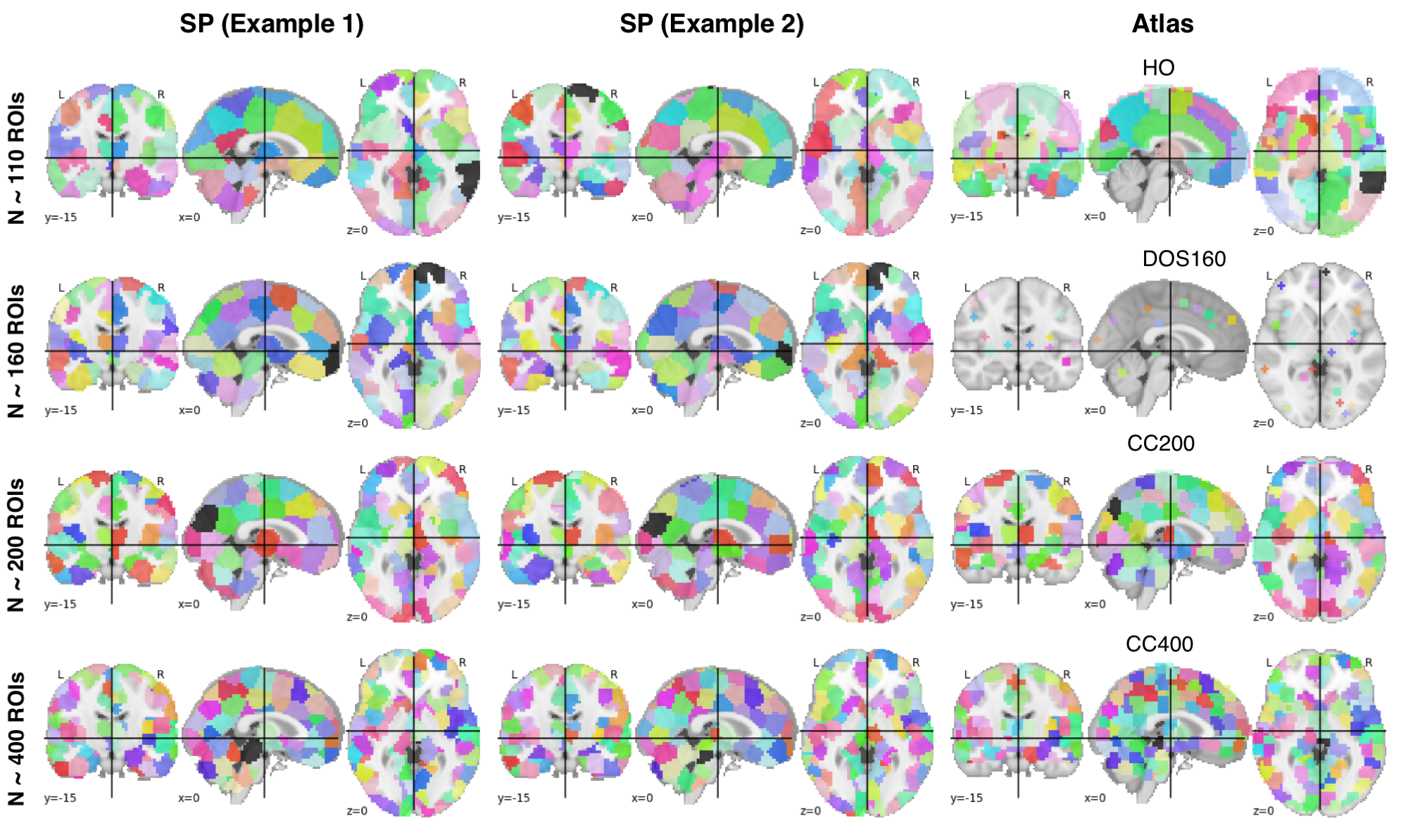
Figure 2: ROI masks for example SPs and atlas at each of the four spatial scales considered in this study.

2.6 3D Convolutional Neural Network Approach

Here, we present our novel strategy to adopt a 3D CNN architecture for use with connectomic data.

Loosely reminiscent of the biological visual system, CNNs use spatially localized filters to detect local image features. Unlike fully connected layers where every unit is connected to all other units of the previous layer, convolutional layers employ a structured arrangement where each unit is connected to only a small subset of spatially connected units in the input image channels. Further, the weights of these connections are shared between the units of the convolutional layer so that the same feature can be detected regardless of its spatial location. Mathematically, a convolutional layer of the form Y=$O_{w}$(X) operates on an M-dimensional input X(v)=($X_{1}$(v),….,$X_{M}$(v)) by applying a set of filters {W={$w_{m,n}$}, m=1,…,M; n=1,…,N}. Here, v is used to index the pixel or voxel (in case of 3D convolution). After applying an elementwise non-linearity $\phi$ (such as a logistic function) , this produces an N-dimensional output Y(v)=($Y_{1}$(v),….,$Y_{N}$(v)). Each element $Y_{n}$(v), known as a feature map, is thus given as,

$$Y_{n}(v)=\phi(\sum_{m=1}^{M}(X_{m}*w_{m,n})(v)),$$ (1)

where * denotes the standard spatial convolution operation.The convolutional layers in CNNs are often interspersed with pooling layers that reduce the size of feature maps and offer translation invariance. Max-pooling is the most popular pooling operation. It down-samples each input feature map (commonly referred to as a channel) separately by selecting the maximum feature response in pre-fixed local neighborhoods. A max-pooling $Y_{i}=P(X_{i})$ operation on channel i is thus defined as, $Y_{i}$(v)=Max($X_{i}$($\bar{v}$): $\bar{v}$ in neighborhood of v). In 3D, for example, the neighborhood can be a 3 x 3 x 3 cube around each voxel. The convolutional and max-pooling layers form the backbone of a CNN. A CNN architecture is constructed by combining multiple layers that successively learn more complex features from the input images. For example, with L layers the output can be mathematically expressed as ($O_{w(L)}$,…P $\circ$ $O_{w(1)}$)(X). Since we are considering an image classification problem, we add fully connected layers to the flattened output at the end of a CNN.

Research in visual recognition has shown that fully connected feedforward architectures don’t scale well to full images. Instead, neural network architectures with local connectivity, such as CNNs, are much more suitable when dealing with high-dimensional images. The shared weights of the CNN architecture facilitate learning with fewer parameters. 3D Convolutional layers thus transform an input 4D (3D multi-channel) volume to an output 4D volume. Each layer learns a set of spatial filters that activate in response to distinct visual patterns. Replicating or convolving each filter across the volume allows the corresponding pattern to be detected irrespective of its spatial location. Finally, the outputs from all filters are stacked along the 4th dimension to create a 4D feature map. Multiple convolutional layers coupled with pooling operations create global representations from local patterns. Stacking fully connected layers at the end after convolutional and down-sampling operations dramatically reduces the model parameter count for classification.

In our proposed approach, the input to the CNN is formed by concatenating voxel-level maps of “connectivity fingerprints”, which are represented as a multi-channel 3D volume. Each channel is a connectivity feature, such as the Pearson correlation between each voxel’s time series and the average signal within a target ROI. In our implementation, we use both atlas-based and stochastic brain parcellation schemes to define target ROIs. The total number of input channels thus represents the number of ROIs used for creating voxel-level fingerprints. For each parcellation scheme (atlas-based or stochastic), we trained a separate model.

In our experiments, we employed a simple CNN architecture, illustrated in Fig. 3. Our architecture has several convolutional layers, interspersed with max-pooling based down-sampling layers, followed by a couple of densely connected layers. The models were trained with a mini-batch size of 64, until convergence of validation loss. For classification, we used binary cross-entropy, whereas for regression we adopted mean squared difference as the loss function. The neural network weights were optimized via stochastic gradient descent (SGD) for classification and Adam for regression. The learning rate and momentum for SGD were set to 0.001 and 0.9 respectively. Learning rate of Adam was set to 0.0005. For age regression, we employ a stochastic weight averaging strategy where we average the neural network weights over last 20 epochs. The same architecture and settings were used for all atlases and stochastic parcellations. We note that each atlas is defined on a unique gray matter mask. To ensure that all prediction models (benchmark and proposed) relied on information from the same voxels, the atlas-specific gray matter mask was applied to the voxel-level connectivity fingerprint data before feeding into the proposed convolutional architecture. For stochastic parcellations, the custom gray matter mask as described above was used for masking the fingerprints. The code and stochastic parcellations have been made available at: https://github.com/mk2299/Ensemble3DCNN_connectomes.

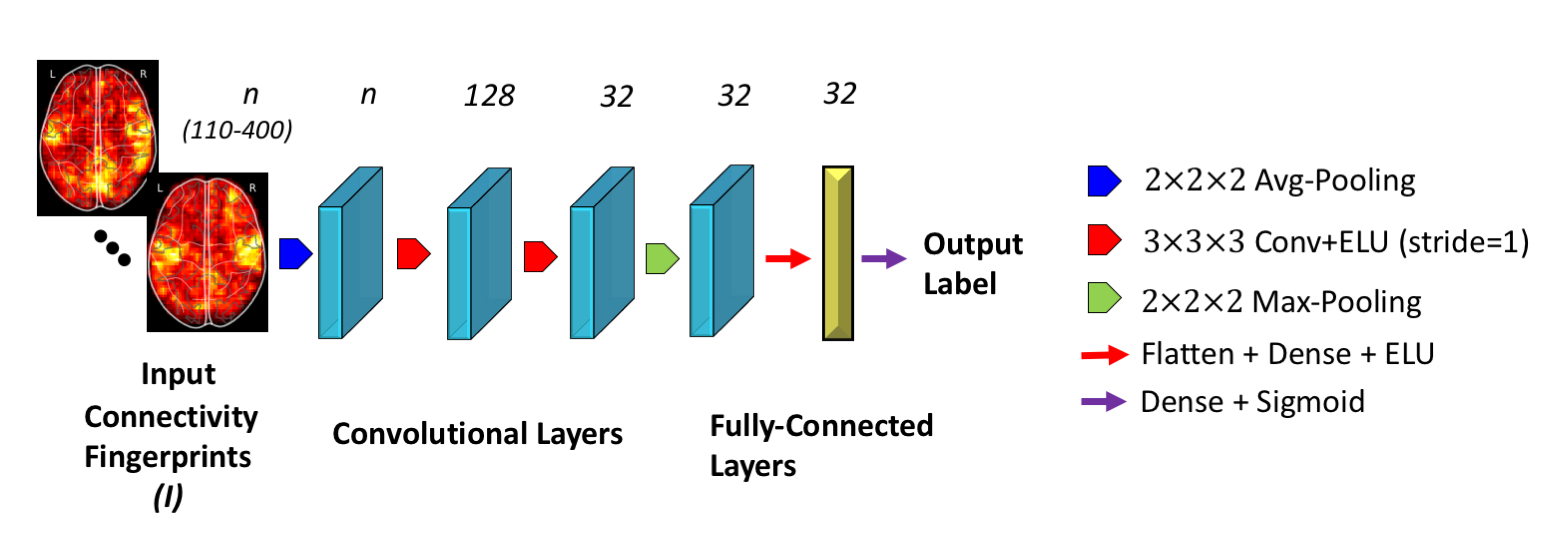
Figure 3: Proposed CNN approach. All operations are in 3D volume. 2D correlation maps are shown for illustration only. For the age prediction task, an additional Max-Pooling and Batch-Normalization[40] operation followed the first and second convolutional layer.

2.7 Benchmark Methods

In our experiments, we implemented following benchmark methods.

2.7.1 Ridge Regression

A linear regression model was trained with squared loss and $\alpha$ times the squared norm of the weight vector (See Appendix). For classification, the ground truth labels were encoded as $\pm$ 1 for the two output categories. We tested 10 linearly spaced values for the hyper-parameter $\alpha$ in the range [0.1,10] and report for the value with the highest cross-validation accuracy.

2.7.2 Support Vector Machine

We implemented a standard SVM as a benchmark (See Appendix). We found that a radial basis function (RBF) kernel performed better than a linear model. Thus we report results for the RBF-kernel SVM. The two hyper-parameters (RBF kernel width $\gamma$ and and misclassification cost weight $C$) were fine-tuned by maximizing cross-validation accuracy via a grid search. For regression, we implemented the standard SVR scheme with an $\epsilon$- insensitive loss function, optimizing for the $\epsilon$-tube and penalty parameter of the error term via grid search.

2.7.3 Fully Connected Architecture

The fully-connected neural network (FCN) architecture takes as input functional connectivity estimates between pairs of ROIs, which is vectorized and processed by a feed-forward network. We implemented following architecture, which performed best on ABIDE-I cross-validation: 4 fully connected hidden layers, with 800, 500, 100 and 20 numbers of features and each linear layer followed by an elementwise Exponential Linear Unit (ELU) activation. Dropout regularization parameter was set to 0.2 and applied to each layer during training. For classification, the output node was a sigmoid, and cross-entropy loss was used. For age prediction, the sigmoidal output was replaced with a linear activation and mean squared difference was used as the loss function. The models were trained with a mini-batch size of 64, until convergence of validation loss.

SGD was used as the optimizer with learning rate and momentum set to 0.01 and 0.9 respectively for classification. For age prediction, a smaller learning rate of 0.001 was used.

2.7.4 BrainNet Convolutional Neural Networks

BrainNet CNN, originally proposed in [20], utilizes specialized kernels to handle connectomic data. Their work described novel edge-to-edge, edge-to-node and node-to-graph convolutional layers that can potentially capture topological relationships between network edges. For BrainNet CNN, we implemented the following architecture that worked best on ABIDE-I cross-validation: 1 edge-to-node layer with 256 filters, followed by a node-to-graph layer with 128 output nodes and finally a dense layer with single output. A leaky ReLU non-linearity with alpha equal to 0.33 was applied to the output of each layer except the last layer. The activation of the last layer was set to linear and sigmoid for the regression and classification tasks, respectively. Dropout regularization with rate 0.2 was used for the edge-to-node layer. Similar to [20], Euclidean loss was minimized for age regression, whereas cross-entropy loss was used to optimize the classification models. The models were trained for 1000 iterations using SGD with momentum equal to 0.9. The learning rate was set to 0.0005 for age prediction and 0.008 for ASD/Healthy classification. The training curves were monitored for atlases to ensure convergence.

2.8 Ensemble Learning

In our experiments, we explored two ensemble learning strategies. The first one is what we call multi-atlas ensemble (or MA-Ensemble). MA-Ensemble averages the predictions of the models of a specific method (e.g., BrainNet CNN) computed using each one of the seven atlases. For classification, the final prediction is computed as the majority vote of the individual binary class predictions. For regression, the ensemble prediction is simply the mean. The second ensemble strategy (SP-Ensemble) averages across the models of a specific method computed using stochastic parcellations. In our experiments, unless stated otherwise, we used 30 stochastic parcellations at each of the following four spatial scales: 110, 160, 200 and 400 ROIs. These scales were chosen in accordance with existing atlases. Thus the SP-Ensemble’s prediction was computed based on fusing 120 ($30\times 4$ scales) models. We also implemented single-scale SP-Ensemble models, which averaged over the 30 parcellations at the same spatial scale.

2.9 Visualizing the CNN model

In order to understand the connectivity features captured by the CNN model, we employed the saliency map approach of [41]. This visualization technique computes the gradient of the output prediction with respect to the input image voxel values, i.e., the 3D volume, using a single backward pass through the trained neural network. We then computed voxel-level saliency as the maximum absolute gradient value across all input channels corresponding to different target ROIs. More formally, consider an input image I, representing the connectivity fingerprints of V voxels with R ROI signals. The saliency weights w $\epsilon\mathbb{R}^{V\times R}$ are computed by taking the absolute value of the gradient of neural network output O with respect to the input image, i.e., $w=|\frac{\partial O}{\partial I}|$. In order to obtain the saliency at the voxel level $S$ $\epsilon$ $\mathbb{R}^{V}$, we take the maximum across all the ROIs, i.e., $S_{i}=\max_{1\leq j\leq R}w_{ij}$. Finally, to visualize an ensemble model, we averaged the individual saliency maps that made up the ensemble.

Table 2: Classification accuracy for ASD vs. Control: Independent test on ABIDE-II of baseline models and proposed CNN approach. For each row, best results are bolded. For each column, best results are italicized. Green indicates better performance, whereas orange/red highlights worse performance.

3 Results

3.1 Experiments

In our experiments, we considered two tasks: i) binary classification of autism vs healthy, and ii) age prediction. For each task, we implemented two evaluation schemes. First, we conducted 10-fold cross-validation on the ABIDE-I dataset, so that we could present results that were comparable to previously reported classification results such as  [1, 18]. Second, we trained each model on the entire ABIDE-I dataset and computed test performance on the independent ABIDE-II set. We report classification accuracy and the receiver operating curves (ROC), along with corresponding area under the curves (AUC) for each of these scenarios under various combinations of parcellation schemes and prediction algorithms. For age prediction, we report the root mean squared error (RMSE).

Table 3: Root mean squared error (RMSE in years) for age prediction: Independent test on ABIDE-II for benchmark models and proposed CNN approach. For each row, best results are bolded. For each column, best results are italicized.

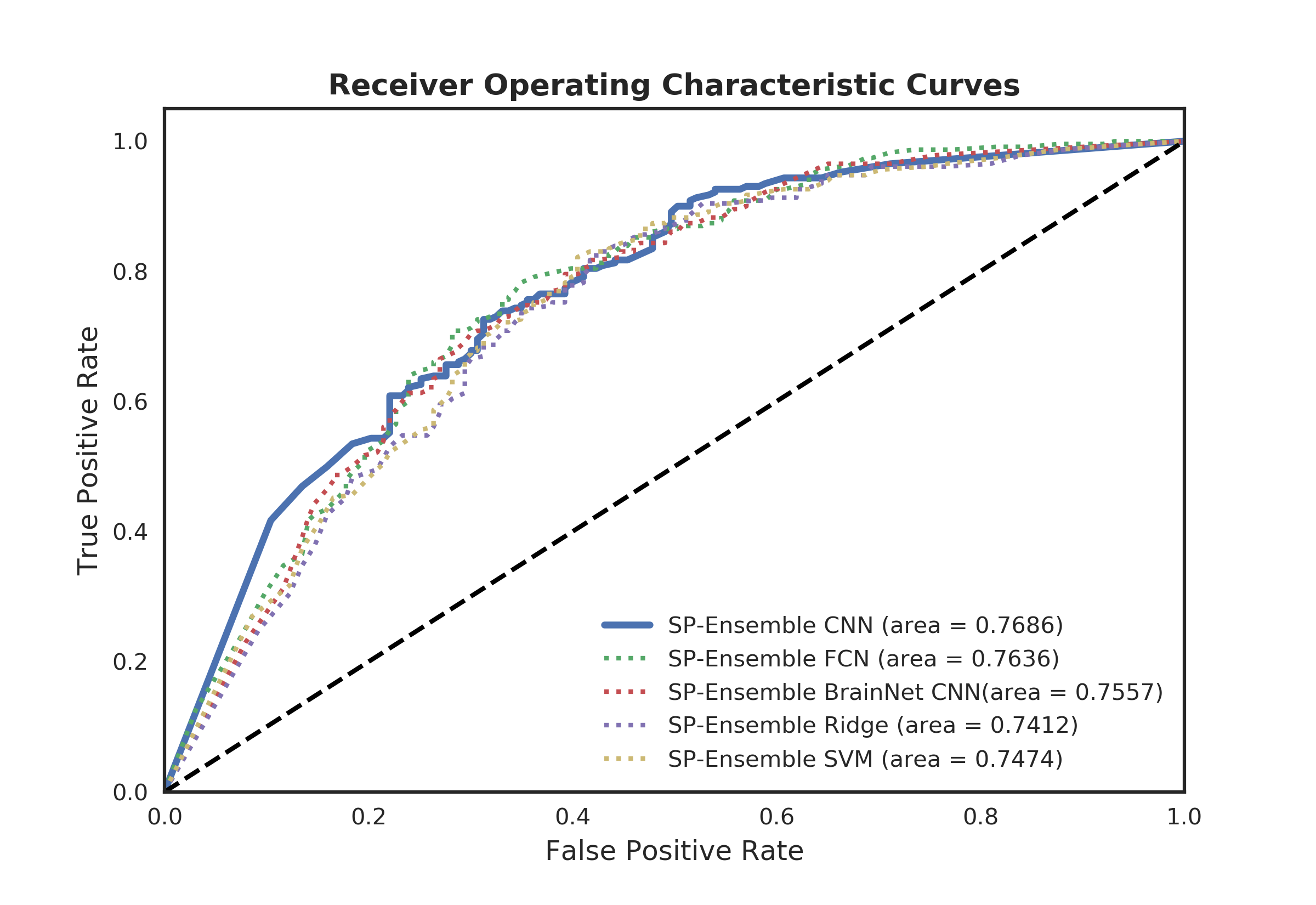
Figure 4: ASD-HC Classification: Receiver Operating Curves for independent validation on ABIDE-2

3.2 Evaluation of Prediction Performance

Table 2 shows the independent test performance for different models on the classification problem. The proposed 3D CNN approach performs at least as good as, and often better than, the benchmark methods, including the fully-connected deep neural network (FCN) and BrainNetCNN. In particular, the 3D CNN approach performs favorably against other algorithms for all but two parcellation schemes, including the ensembles. Similarly, the SP-Ensemble achieves the best ABIDE-I cross-validation for most algorithms, including the 3D CNN. The ABIDE-I cross-validation results, reported in Table S.2, are in general compatible with the independent test results, where the 3D CNN and SP-Ensemble techniques mostly outperform the competition. Figure 4 shows the Receiver Operating Characteristic (ROC) curves for SP-Ensemble models for the different algorithms on the independent ABIDE-II test dataset. We observe that the 3D-CNN SP-Ensemble achieves an AUC of $\sim 77\%$ and an accuracy of $\sim 72\%$ on independent ABIDE-II data, slightly better than the state-of-the-art cross-validation on ABIDE-I for ASD/HC classification [24], with FCN and Brain-Net CNN ensembles yielding a similar performance. ROC Curves for individual atlases are shown in Figure S.4.

Table 3 lists independent test results for the age prediction task on ABIDE-II, and Table S.3 reports the 10-fold cross-validation error on ABIDE-I. The 3D CNN approach consistently shows superior performance, yielding the best results for all parcellation schemes. Similar to the classification scenario, SP-Ensemble or MA-Ensemble also yield the best cross-validation and independent test performance values for the majority of the algorithms, including 3D CNN. Overall, the best accuracy is achieved by SP-Ensemble 3D CNN, which yields a root mean squared error of 3.28 years on ABIDE-I cross-validation and 2.15 years on the independent ABIDE-II dataset. We also estimated mean absolute error (MAE) of all models on ABIDE-II and observed a similar trend, as reported in Table S.6.

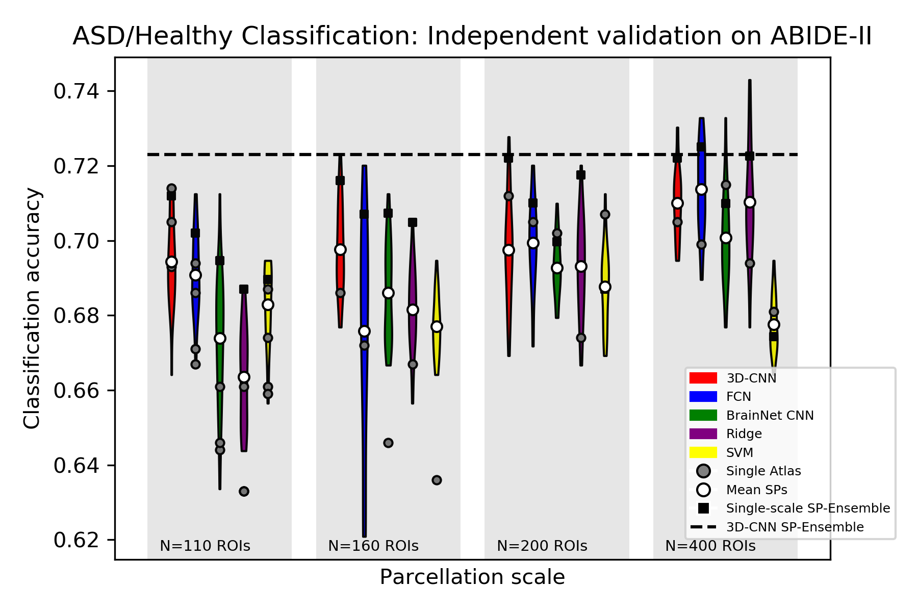
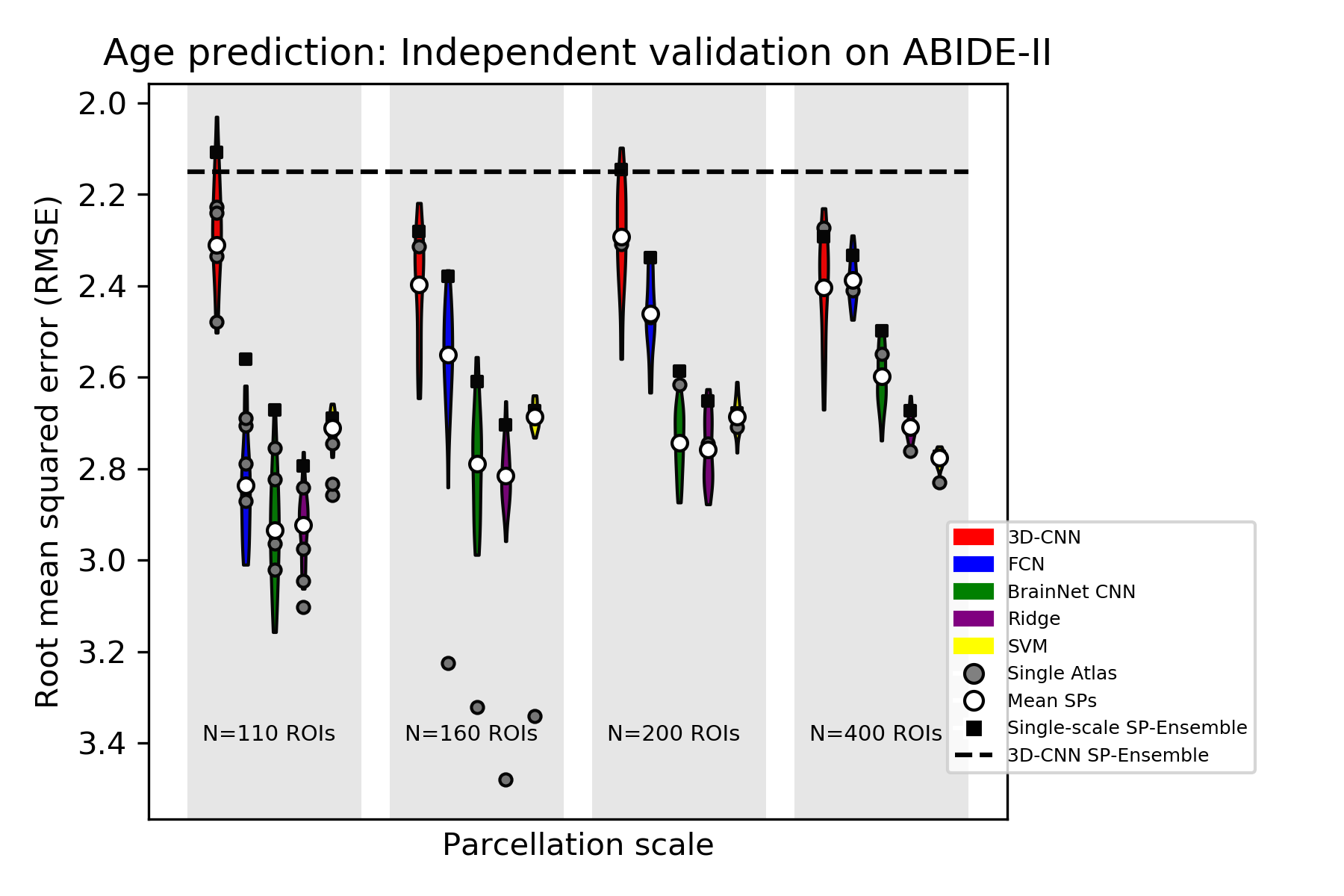
Figure 5: Violin plots showing the spread of prediction accuracies/errors for stochastic parcellations at multiple network scales for different classification models. Mean accuracy/error of individual violins is denoted by ’Mean SPs’. Performance of individual atlases is compared with SPs with the closest # of ROIs and is denoted as ’Single Atlas’. Results are computed by training models on entire ABIDE-1 cohort and testing on the independent ABIDE-2 cohort.

3.3 Comparison of stochastic parcellations and atlases

Here, our objective is to conduct a detailed investigation of how the choice of ROIs affects prediction performance for different machine learning (ML) algorithms. For each ML algorithm and each parcellation we have a model trained on the ABIDE-I data, which we then used on the independent ABIDE-II data to quantify prediction accuracy. Figure 5 shows the distribution of accuracy values (estimated with a kernel density model) obtained using stochastic parcellations , while also illustrating the results for each of the atlases and the scale-specific SP-ensembles. The scale-specific SP-Ensemble strategy, as the name implies, averaged the models corresponding to the 30 stochastic parcellations in each scale. We observe that the atlas-based models performed no better than typical stochastic parcellation models, independent of scale and algorithm. This result offers an intriguing possibility: perhaps we do not need anatomically or functionally derived brain parcellations to train machine learning models since stochastic parcellations perform equally well or no worse in practice.

Our proposed SP-Ensemble CNN strategy yielded accuracy results that were about as good as the best scale-specific SP-Ensemble model. Finally, the ensemble models were almost always better than the atlas-based models and they compared favorably against the individual stochastic parcellation models. The same observations can be made for ABIDE-I cross-validation (see Supplementary Figure S.1).

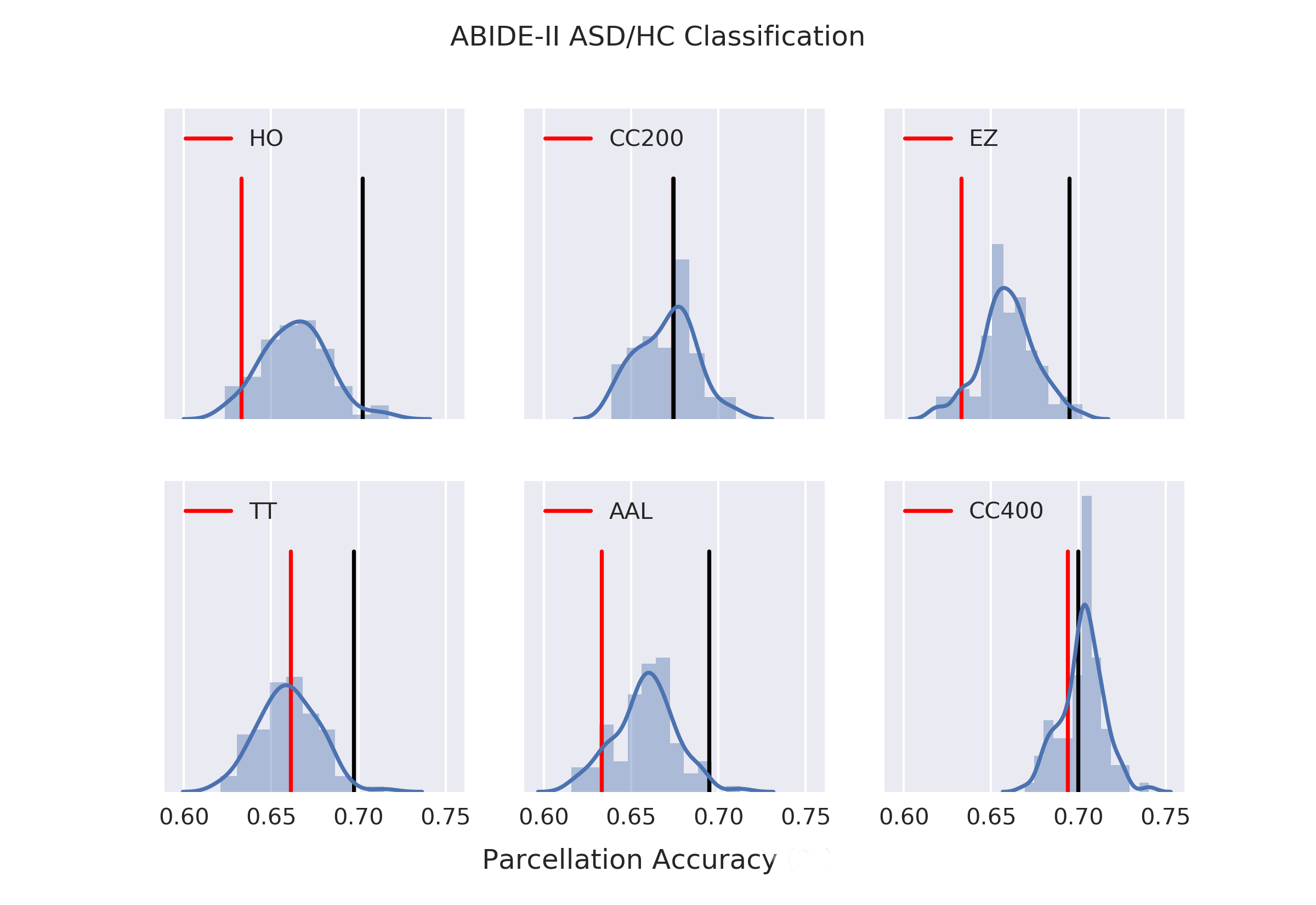
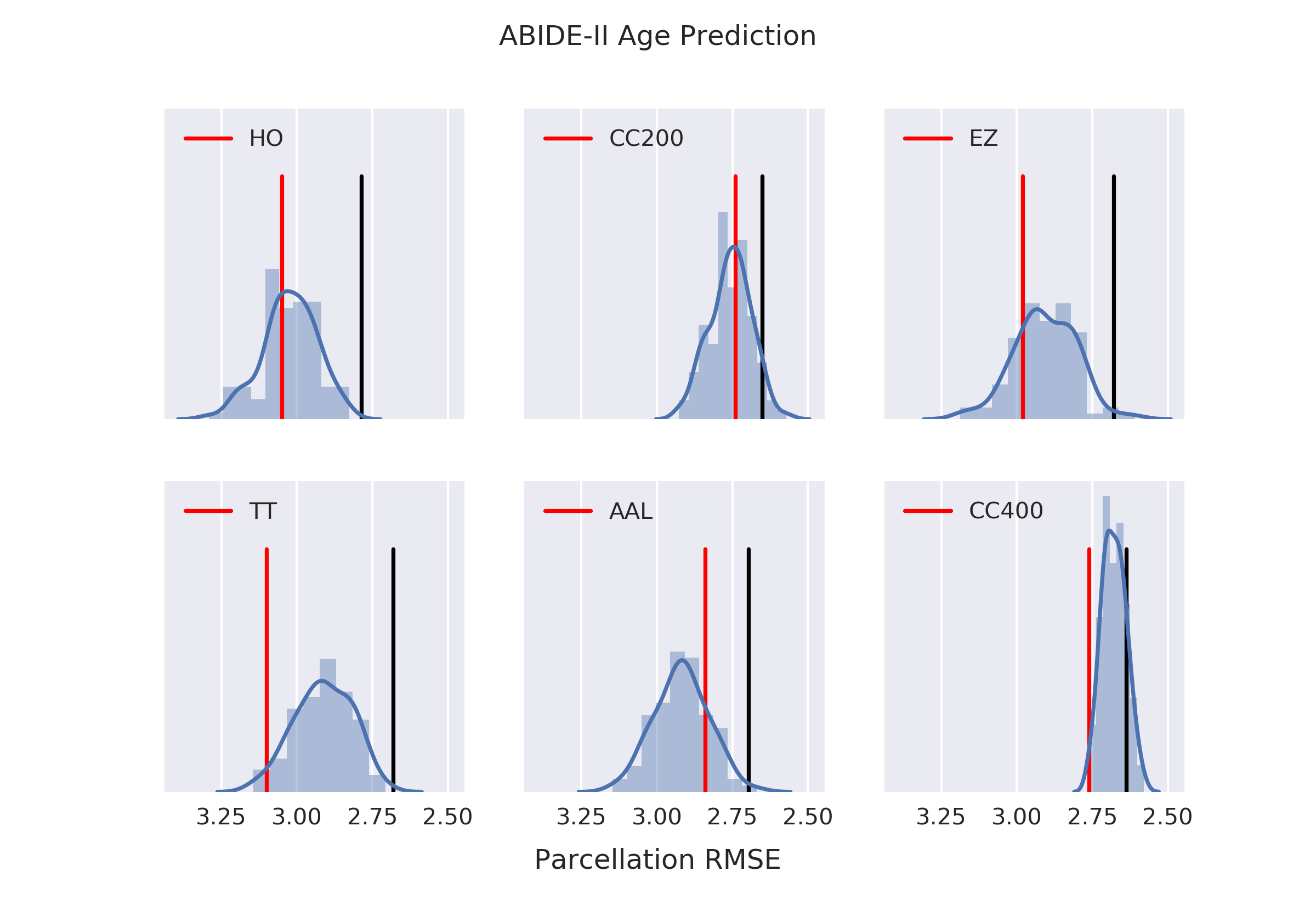
Figure 6: Distribution of Ridge models’ performance for stochastic parcellations created using the same gray-matter mask as the corresponding atlas. Red denotes the atlas model’s accuracy and black indicates the SP-Ensemble accuracy.

In above analysis, one potential confound was the different gray matter masks of atlases and stochastic parcellations (SPs). In order to account for this confound, we conducted following analysis. For each of the atlases, we generated 100 SPs using the same gray matter mask as the atlas. We excluded DOS160 because it does not rely on a well-defined gray matter mask and places discontiguous 4.5 mm spherical regions over fixed coordinates in the brain (sampling only 5% of brain voxels). We then trained on each of these SPs using the same hyper-parameters that were found to be optimal for the corresponding atlas. Here, we show the results for ridge regression (the model that was fastest to train), but we obtained similar results for all other algorithms as well. As can be seen from Figure 6, for most atlases and corresponding gray matter masks, the model trained on the atlas ROIs performed no better than an average SP model. Furthermore, and importantly, the SP-Ensemble (computed by averaging across SPs on the atlas-specific mask) yielded better performance than the atlas models for all atlases.

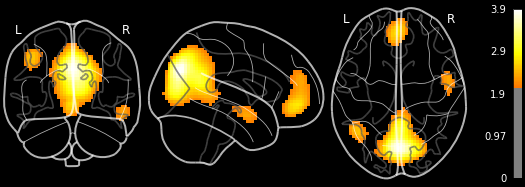
(a) ASD/Healthy Classification

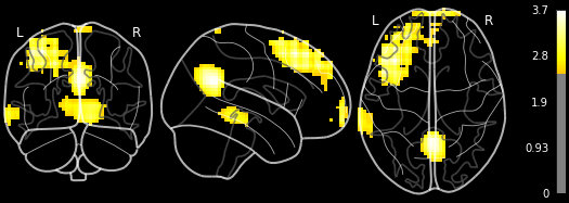
(b) Age prediction

Figure 7: Mean saliency maps of trained 3D-CNN models for SP-Ensemble

3.4 Visualization

An important goal of machine-learning tools in neuroimaging is to generate novel insights linking imaging biomarkers with disease or phenotypic traits. Visualization techniques for CNNs can help reveal important features used by the model for discriminating between output classes. Figure 7 shows the saliency maps computed for the SP-Ensemble CNN ASD classification and age prediction models. As can be seen from these maps, the precuneus, often considered a core node of the default mode network [42], seems to play a significant role for both prediction problems. However, there are also salient regions that are unique to each problem. For example, the anterior cingulate/ventromedial prefrontal cotex, a region that has been linked to autism [43], was distinctly highlighted for the ASD classification problem. The left parietal cortex was also emphasized for ASD prediction, which is consistent with the laterilized activation observed in this region in Autism patients [44]. On the other hand, for age prediction, the left dorsolateral prefrontal cortex (dlPFC) is a uniquely salient region. The dlPFC is associated with executive functions, such as working memory and abstract reasoning. For working memory, dlPFC’s function seems to be age-associated and more lateralized in younger adults [45].

4 Discussion

In this study, we presented a detailed empirical analysis of how the choice of ROIs can impact the performance of machine learning models trained on functional connectomes. We considered several machine learning algorithms, together with a range of spatial scales and parcellation schemes, including the popular atlas-based techniques and a stochastic approach. Our analysis suggests that using a single atlas for summarizing the connectome data is often sub-optimal for training machine learning models, and significantly more accurate predictions can be achieved with an ensemble approach that averages across models trained with different parcellation schemes. Furthermore, we demonstrated that averaging across stochastic parcellations can achieve very high accuracy values, often surpassing atlas-based models. Our findings resonate with several other studies that compare stochastic parcellations and atlases, although in different contexts. Craddock et al. [46] compared spatially constrained functional parcellations obtained from spectral clustering with anatomically constrained parcellations produced from random clustering. Random parcellations performed as well as functional parcellations and better than anatomical atlases on metrics of cluster homogeneity and representation accuracy. Based on this, the study reflected that sufficiently small ROIs perform well for functional network analysis regardless of their spatial position. Fornito et al. [47] generated stochastic parcellations by randomly sub-dividing the AAL atlas and showed that functional organizational properties are independent of the parcellation template at the same network resolution, although significant variability is observed across scales. Studies on diffusion-MRI based anatomical networks have similarly shown that topological attributes and network organizational parameters are consistent across different parcellation schemes, including random parcellations [48, 39].

Another main contribution of this study is a novel approach to employ a 3D CNN architecture on functional connectivity data. Convolutional neural networks achieve state-of-the-art performance on many image-based prediction tasks, as they take advantage of the full spatial resolution of the data and the translation invariance property of the problem. Our proposed approach treats voxel-level connectivity fingerprints as input channels to a conventional 3D CNN framework. Spatial convolutions can capture local structural or topographic patterns in the data, such as connectivity gradients. Successively stacking convolutional layers in our architecture would hierarchically yield higher-order features that can capture information relevant for classification. Studies have shown that individual-level network topography serves as a fingerprint of human behavior [49]. Our multi-channel input image comprising connectivity fingerprints, coupled with CNNs, provides a natural framework to capture individual-level differences in topography as they relate to behavior or disease. This strategy contrasts with current practice where the input to machine learning models are pairwise ROI functional correlations. This makes the model more susceptible to uncertainty caused by parcellation choice. This can be seen in our experiments where there is relatively larger variance in prediction performance across atlases for the fully-connected neural network. Thus, CNNs with connectivity map inputs can offer a more robust alternative to classification approaches that only rely on ROI-level connectivity information, such as the BrainNet-CNN. Our results demonstrate that when tailored for connectomes, CNNs offer a promising opportunity to probe brain networks in disease.

Machine learning practitioners have to make a number of preprocessing choices in extracting connectomic features to analyze. While there is no one-size-fits-all solution across different tasks, in the context of machine learning models of functional connectivity, we present some interesting empirical observations below.

4.1 Ensemble learning

The motivation behind using multiple stochastic parcellations for prediction is grounded in the concept of ensemble learning. The core idea is to integrate out a latent variable (i.e., parcels or ROI definitions) from the learning problem [50]. This approach also makes the predictions more robust to the precise parcellation scheme. As shown above, the performance of atlas-based models can vary significantly ($\sim$5-10% for parcellations at the same scale). In such a scenario, ensemble learning over multiple stochastic parcellations can be a robust strategy that yields reliable predictions.

4.2 Network granularity

We explored the impact of network granularity on prediction performance of machine learning algorithms for connectomes. Our analysis suggests that better prediction performance can be expected with parcellations at higher granularity upto $\sim$ 400 ROIs. To further investigate this trend on ROI-level models, we trained the fully-connected network (FCN), that is generally the best performing baseline algorithm, on both the prediction tasks for the 1024 node parcellation proposed in [48]. As can be seen from Table 4, an atlas with 1024 regions is comparable to the CC200 atlas for ASD/HC classification in ABIDE-II. However, the performance actually degrades significantly (in comparison to CC200 or CC400) for the age prediction task.

Table 4: Classification/regression performance of FCN with a high-resolution parcellation ( $\sim$ 1024 ROIs) [48]

Our evaluations contradict with a previously reported result that a coarser network scale ($\sim$ 100-150 ROIs) is more suitable for autism classification [18]. In their paper, these conclusions were drawn by comparing the performances achieved with a few atlases. However, inferring trends from a small number of atlases can be misleading, since factors like the boundary definitions of structures (cortical/subcortical) or the particular gray matter mask used, will effect results. Stochastic parcellations can control for these confounds and depict unbiased trends across network scales.

4.3 Number of gray matter voxels

Our empirical study suggests that there is no direct correlation between the number of voxels in the gray matter mask and a model’s prediction performance. However, we do observe that the choice of gray matter mask can impact results. For example, the DOS160 atlas with as few as $\sim$ 3,039 voxels shows performance no worse than other atlases at the same resolution (HO, EZ, TT and AAL) with $\sim$ 20x more voxels.

4.4 Visualization

Saliency maps provide a valuable visualization strategy to probe deep neural network models. We visualized the saliency maps from 3D CNN models trained on ROIs extracted using both atlases and stochastic parcellations. As shown in Figure 7 and Supplementary Figures S.2 and S.3, these maps are remarkably consistent.

These maps reveal that the precuneus, which is a hub of the default mode network and associated with ASD and age, plays an important role for both prediction problems. There were also uniquely highlighted regions, such as the anterior cingulate/ventromedial prefrontal cortex for ASD classification and the left dorsolateral prefrontal cortex (dlPFC) for age prediction. Several studies have suggested the potential of DMN connectivity as a neurophenotype of autism. Chen at el. [51] trained a random forest classifier that distinguished ASD subjects from healthy controls with high accuracy, and showed that default mode and somatosensory regions contribute significantly to diagnostic accuracy. Similarly, Abraham et al. [18] revealed discriminative connections in the DMN for ASD/HC classification within a larger heterogeneous cohort of the ABIDE dataset. Furthermore, it has been shown that the connectivity of posterior cingulate cortex (PCC) and aberrations in the medial prefrontal cortex node of the DMN can predict social deficits in children with ASD [52]. Our results corroborate the findings of these studies, and suggest a crucial involvement of DMN in autism.

4.5 Influence of motion

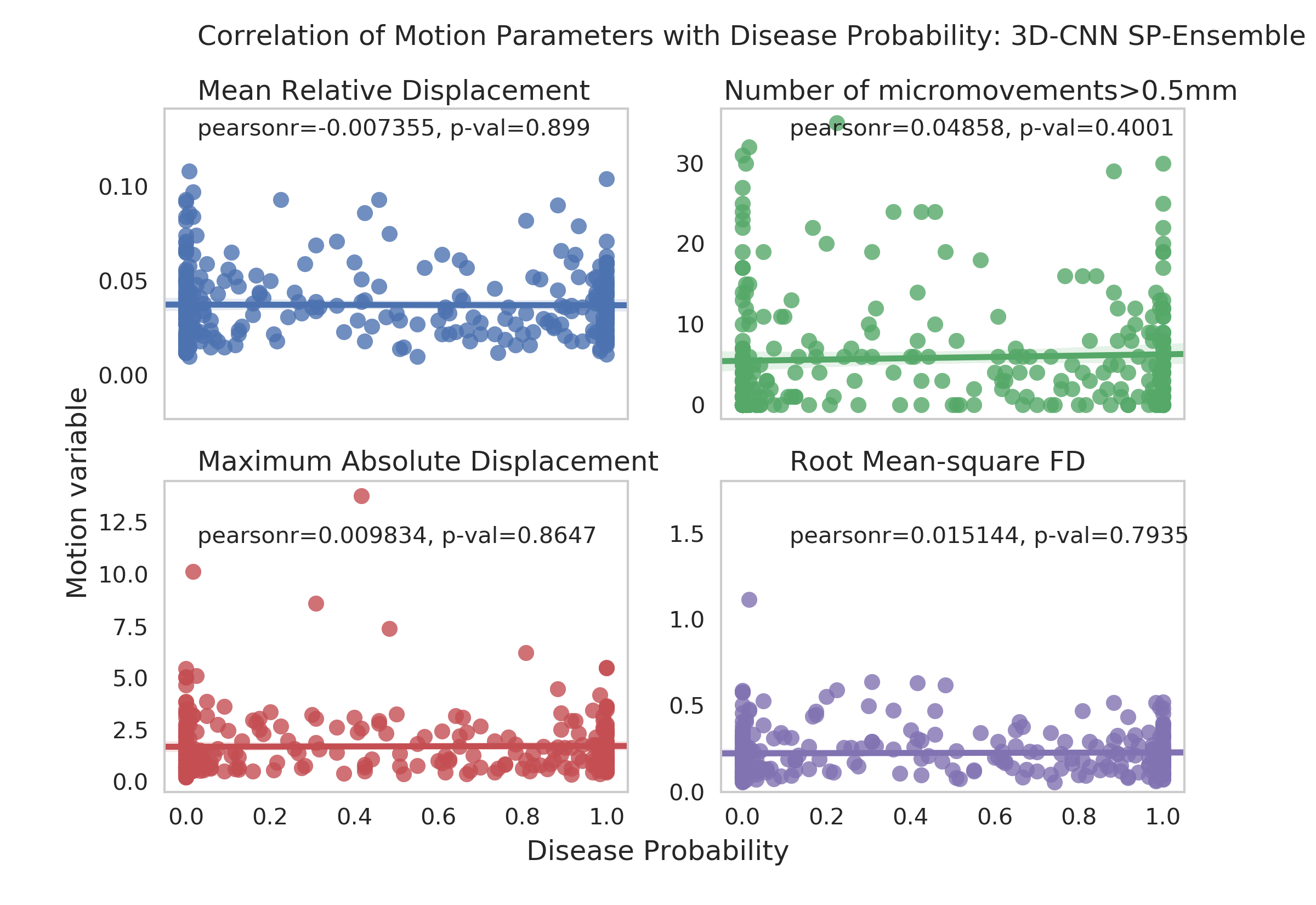
Figure 8: Motion correlations

Several studies have shown differences in head motion parameters during fMRI between healthy controls and diseased populations, or between subjects from different age groups [53, 54]. This, in turn, can manifest as artifacts in the derived resting-state connectivity [55]. Although our independent test data was motion scrubbed, we performed additional analyses to rule out the confounding effect of motion in classifier decisions. We selected a cohort of 151 ASD subjects with motion-matched healthy controls from our independent dataset and analyzed the correlation of 4 motion parameters with classifier predictions. These include the root-mean-square framewise displacement, mean relative displacement, maximum absolute displacement and the number of micro-movements greater than 0.5mm. These summary statistics were chosen in accordance with previous reports of motion artifacts in rs-fMRI[28]. As shown in Figure 8, no significant correlations were observed between motion variables and the predictions of SP-Ensemble (model average over all atlases). In this motion-matched cohort, classification accuracy of 71.8% was obtained using 3D-CNN.

For our regression task, there was no significant correlation between a subject’s age and any of these motion parameters in our cohorts.

4.6 Recommendations

Based on our experiments, we make two claims in this study: (a) 3D-CNN performs favorably compared to alternative baseline algorithms, and (b) Ensemble models that average across parcellation schemes consistently perform better than individual atlas-based models and are thus a safer choice for supervised machine learning on connectomes. This is because individual atlases can show significant variability in classification/regression performance and finding the optimal atlas for a prediction task among the wide range of available atlases might not be feasible. Figure 9 shows the probability density estimates for the difference in performance between (a) 3D-CNN versus baseline algorithms as evaluated with the SP-Ensemble strategy, and (b) SP-Ensemble versus single atlas implemented with the 3D-CNN model. These estimates are presented for both our prediction tasks. For this experiment, we estimate the evaluation metrics (AUC-ROC for ASD/HC classification and RMSE for age regression) on 10,000 bootstrapped samples from ABIDE-II. These results demonstrate that the SP-Ensemble approach consistently achieves an accuracy as good as the best performing single-atlas model. Further, the 3D-CNN model consistently outperforms the baseline algorithms for the age prediction task, with more prominent improvements for individual atlas models. This can be seen from Tables 2 and 3. We note that when using the ensemble strategy, the differences between models are marginal and might be irrelevant in some practical applications. For instance, the SP-Ensemble performance on ASD/HC classification task is comparable among 3D-CNN, FCN or BrainNet-CNN, with slight improvements over linear models. Thus, if time and/or computational resources impose constraints, it might be more suitable to prefer simpler models like FCN or SVM over 3D-CNN for example, especially with the ensemble approach.

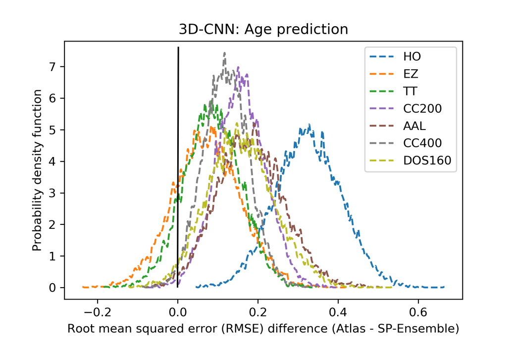
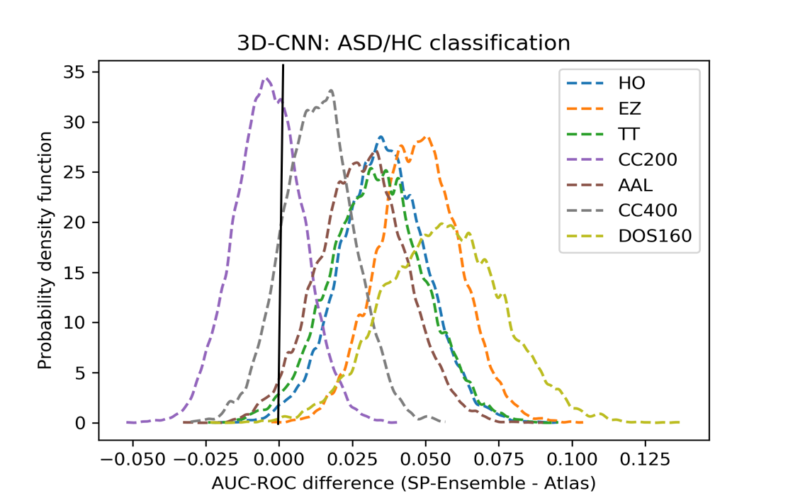
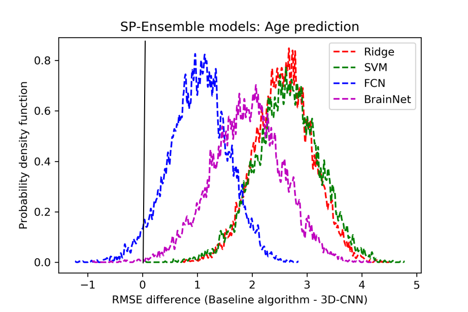
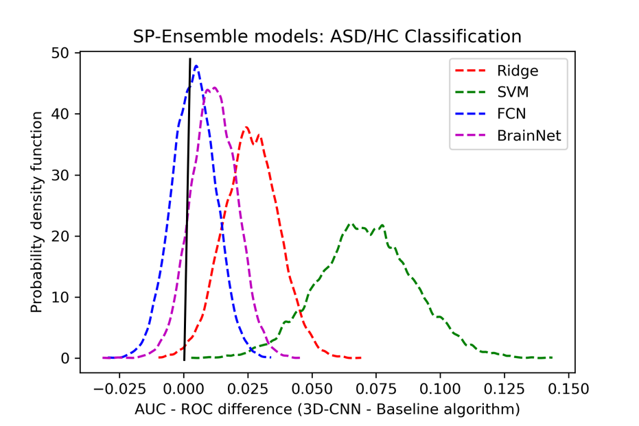
Figure 9: Kernel density estimates of the probability distributions for the performance difference between models, computed based on 10000 bootstrap samples from ABIDE-II. Values to the left of the black vertical line indicate bootstrap samples where the proposed approach (3D CNN or SP-Ensemble) under-performed compared to the competing method.

4.7 Limitations and future work

Throughout our analysis, Pearson’s correlation was chosen to measure functional connectivity strength between different brain regions. Several other correlation metrics, including tangent-based and partial correlation have been shown to yield superior classification performance in prior studies [9, 18]. While we do not expect this to affect the general conclusions and findings of our study, the choice of the correlation metric still remains an arbitrary decision in any machine learning pipeline for connectomes.

Due to the heavy computational burden required for training multiple deep learning models, we only considered one particular scheme for creating stochastic parcellations, i.e., Poisson Disk Sampling. Alternative strategies for creating random parcellations have also been proposed, for instance, through stochastic sub-division of anatomically derived ROIs into smaller parcels [56]. It is also possible to randomize several other more popular schemes for parcellating the brain, such as, using Ward’s clustering on functional data from sub-samples of the population [50] or creating Geometric parcellations with different initializations [13].

While the proposed CNN approach achieves promising accuracy on autism detection and age prediction, there is room for further improvement. We have not yet conducted a comprehensive optimization of the convolutional architecture. Furthermore, there are likely more optimal choices than target ROI-based correlations that are used as input to the model. An interesting alternative would be select random gray matter vertices for connectivity profiling, as proposed in [16]. We envision an end-to-end learning strategy that can enable the optimization of these connectomic features.

Saliency maps provide an appealing visualization technique by mapping the neural network activations back to input voxel space. Several modifications to gradient-based back-propagation have been reported in literature that can potentially highlight more informative features learnt by the model [57, 58]. Further, the use of saliency maps need not be restricted to depicting group-averaged discriminative features. Unsupervised learning on saliency maps can provide novel insights into clinical subtypes of disease. It is also important to note that machine learning techniques do not unequivocally provide evidence for the salient features being directly associated with the disease or other target variables. However, when combined with detailed future investigations, they can spur clinical discoveries.

4.8 Conclusion

The results presented in our paper showcase the utility of ensemble learning for connectomes. Functional network based prediction models are impacted by several a priori choices, the most pivotal of which is the ROI definition. We demonstrate that ensembles of stochastic parcellations yield predictions that are significantly more robust and accurate compared to single atlas-based approaches. Further, our experiments highlight the potential of convolutional neural network models for connectome-based classification.

5 Acknowledgements

This work was supported by NIH grants R01LM012719 (MS), R01AG053949 (MS), R21NS10463401 (AK), R01NS10264601A1 (AK), the NSF NeuroNex grant 1707312 (MS) and Anna-Maria and Stephen Kellen Foundation Junior Faculty Fellowship (AK).

6 References

7 Supplementary Material

7.1 Atlas Summary

Atlas	$\#$ of ROIs	Total Vol.	Median Vol.($\pm$ std)	Min Vol.	Max Vol.
TT	97	1656.34	12.5 ($\pm 16.02$)	0.03	69.71
HO	111	1611.39	10.04 ($\pm 15.26$)	0.05	97.33
EZ	116	1941.65	14.11 ($\pm 11.96$)	0.97	56.35
AAL	116	1843.10	13.78 ($\pm 11.05$)	1.35	53.33
DOS160	160	82.05	0.51 ($\pm 0.04$)	0.03	0.51
CC200	200	1172.15	5.83 ($\pm 1.26$)	1.81	9.96
CC400	400	1172.15	2.97 ($\pm 0.68$)	0.76	5.35

Table S.1: Summary descriptors of ROIs in individual atlases. All volumes are in $cm^{3}$.

7.2 Poisson Disk Sampling

Poisson disk sampling is a stochastic sampling procedure where drawn samples are required to be at least a distance d apart for some user-specific distance metric and density parameter. Since we use this sampling procedure to draw parcel centers, d is estimated a priori based upon the desired number of parcels, and spatial proximity is used to compute the distance. We use the fast poisson disk sampling algorithm as proposed in [59]. This is an efficient sampling procedure that generalizes to arbitrary dimensions and allows volumetric sampling. The algorithm is outlined below:

• Step1: A parcel center is arbitrarily chosen from all gray matter voxels and stored in an initially empty ‘active’ list.

• Step 2: A sample c is drawn from this active list of voxels. The next candidate parcel center is randomly selected from the list of all voxels within a spherical annulus between radius d and 2d around c. A candidate is accepted and added to the active list if it is atleast a distance d apart from all the existing parcel centers; otherwise another candidate is chosen. If no candidate is accepted from the annulus, c is removed from the active list and another sample c is drawn. This procedure is repeated until the active list is empty.

• Step 3: Once the centers are sampled, every gray matter voxel is assigned to its closest parcel center. Sampling is performed for the left and right hemispheres separately to avoid parcels that cross hemispheric boundaries.

7.3 Linear Classifiers

7.3.1 Ridge Classifier

Given feature vectors $x_{i}$ for n subjects and the corresponding prediction variables denoted by $y_{i}$, we approximate the fit using a linear regression model. An $L_{2}$ regularization for the weights (w) is added to the mean squared error to yield the following loss function of ridge regression:

$$\mathcal{L_{R}}=\left\|Xw-y\right\|^{2}+\alpha\left\|w\right\|^{2}$$ (2)

During classification, the output labels y are encoded as $\pm$ 1 for the two output categories to minimize the above loss.

7.3.2 Support Vector Machines

(a) Classification
Support Vector Machine Classifiers optimize for a hyperplane with maximum margin between the output classes. This results in a decision function of the form, f(x)= sign($w^{T}x+b$). The weights {w, b} are obtained by minimizing the following convex loss function consisting of a data loss component ($\mathcal{L_{D}}$) and a regularization loss for the weights ($\mathcal{L_{W}}$),

$$\mathcal{L_{SVC}}=C\mathcal{L_{D}}+\mathcal{L_{W}}$$ (3)

$\mathcal{L_{D}}$ is modeled using a hinge loss function, $\sum_{i=1}^{n}$max$(0,1-y_{i}(w^{T}x_{i}+b))$ over all n training samples {($x_{1}$,$y_{1}$),…,($x_{n}$,$y_{n}$)}. $\mathcal{L_{W}}$ is modeled using a Euclidean norm, i.e., $\left\|w\right\|^{2}$. Here, C is a tuning parameter that controls the trade-off between regularization and data loss.
(b) Regression
The $\epsilon$-Support Vector Regression (SVR) scheme optimizes for a decision function of the form, f(x)=$w^{T}x+b$, that has at most $\epsilon$ deviation from the true prediction variables y (allowing for errors when the problem is infeasible). The loss function ($\mathcal{L_{SVR}}$) can be formulated as,

$$\mathcal{L_{SVR}}=C\mathcal{L_{\epsilon}}+\mathcal{L_{W}}$$ (4)

$\mathcal{L_{\epsilon}}$ is traditionally referred to as the $\epsilon$-insensitive loss function, and is formulated as $\sum_{i=1}^{n}$max$(0,|w^{T}x_{i}+b-y_{i}|-\epsilon)$ over all n training samples {($x_{1}$,$y_{1}$),…,($x_{n}$,$y_{n}$)}. The regularization term ($\mathcal{L_{W}}$) is modeled using a Euclidean norm, i.e., $\left\|w\right\|^{2}$. The tuning parameter C controls the trade-off between the regularization (i.e., the flatness of the decision function) and the amount up to which deviations beyond $\epsilon$ are tolerated.
Both the classification and regression problems yield weights w that can be represented completely as a linear combination of the training inputs $x_{i}$. Thus, w is represented as $\sum_{i=1}^{n}\alpha_{i}x_{i}$, and the decision function becomes f(x)=$\sum_{i=1}^{n}\alpha_{i}x_{i}^{T}x+b$. This makes it easier to extend SVMs for non-linear decision functions using the kernel technique, i.e., by applying transformations $\phi$(x) that map x to a high-dimensional space and replacing the inner product $\langle x_{i},x\rangle$ with the kernel $K(x_{i},x)$=$\langle\phi(x_{i}),\phi(x)\rangle$. For our experiments, we observed that the radial basis function kernel, $K(x_{i},x)=$exp(-$\frac{\left\|x_{i}-x\right\|^{2}}{2\sigma^{2}})$, yields the best results among linear, sigmoid and polynomial kernels up to degree 4.

7.4 Neural network hyperparameter settings

We note that since it is more expensive to train a 3D-CNN, we could experiment with only a limited configuration of hyperparameters during cross-validation on ABIDE-I data, compared to FCN and Brain-Net CNN, which work with vectorized connectivity matrices and are thus faster to train. For all three neural network models, we relied on a random search over the learning rate, number of layers, number of units or feature maps in each layer and the choice of non-linearity. For this search we employed the HO atlas. The hyper-parameter configuration that yielded the best ABIDE-I cross-validation accuracy was subsequently used for all other parcellation schemes. Note that except for some minor changes, the models for age prediction and ASD/HC classification are almost identical. Furthermore, in our primary analyses we compare models based on ABIDE-II performance, which was not used for hyper-parameter tuning.

For the FCN, we initially started with the architecture proposed by Heinsfeld et al.[24] for ASD/HC classification. We increased the number of layers before the softmax output until the ABIDE-I cross-validation accuracy stopped improving. Also, we noticed that adding batch-normalization after each layer had no noticeable impact on classification performance. Hence, we didn’t include this layer in our FCN architecture.

7.5 ABIDE-I cross-validation results

Table S.2: Classification accuracy for ASD vs. Control: 10-fold cross-validation on ABIDE-I for benchmark models and proposed CNN approach. For each row, best results are bolded. For each column, best results are italicized. Green indicates better performance, whereas orange/red highlights worse performance.

Table S.3: Root mean squared error (RMSE in years) for age prediction: 10-fold cross-validation on ABIDE-I for benchmark models and proposed CNN approach. For each row, best results are bolded. For each column, best results are italicized. Green indicates better performance, whereas orange/red highlights worse performance.

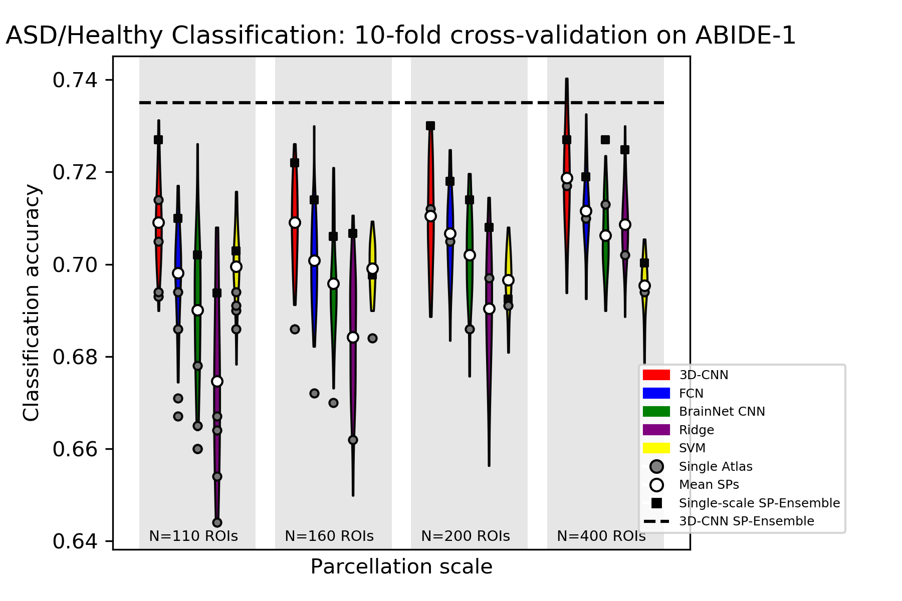
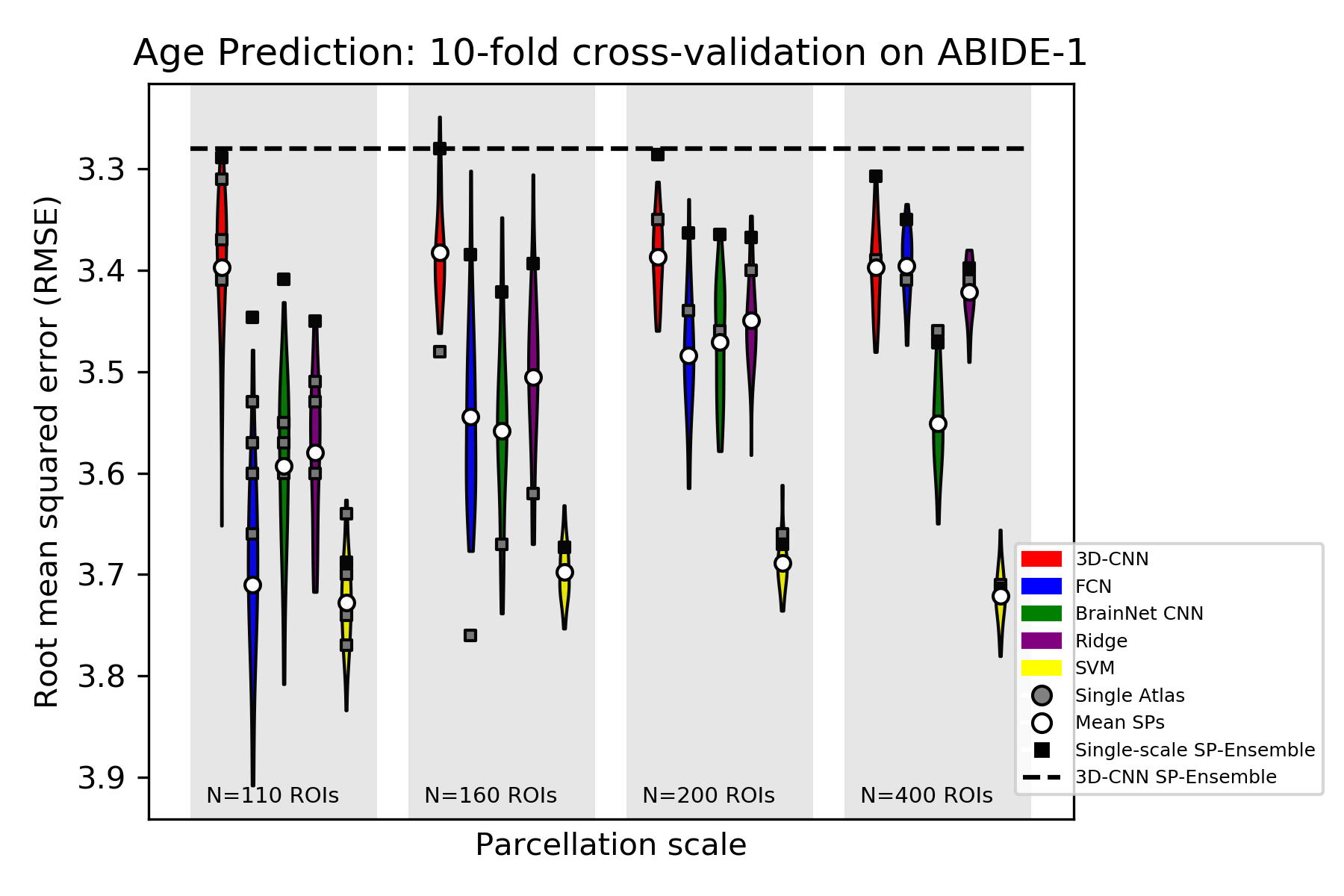
Figure S.1: Violin plots showing the spread of prediction accuracies/errors for stochastic parcellations at multiple network scales for different classification models. Mean accuracy/error of individual violins is denoted by ’Mean SPs’. Performance of individual atlases is compared with SPs with the closest # of ROIs and is denoted as ’Single Atlas’. Results are computed by 10-fold cross-validation on the entire ABIDE-1 cohort.

In order to ensure a fair comparison with other studies that report 10-fold cross-validation performance on ABIDE-I, we report the performance obtained using our benchmark and proposed models (along with the ensemble learning strategy) for both stochastic parcellations and atlases in the form of kernel density plots (Figure  S.1 and Tables S.2, S.3). Clearly, the results and conclusions on ABIDE-I remain consistent with ABIDE-II, with the 3D-CNN ensemble strategy outperforming all the baseline methods.

7.6 Saliency maps for individual parcellations

Visualizing the saliency maps for models trained on different brain parcellations can reveal interesting differences in the features captured by these models. We visualized the saliency maps of the 3D-CNN model for individual stochastic parcellations at multiple scales for the task of ASD/HC Classification. As shown in Figure S.2, models trained using distinct parcellation schemes are relying on the same basic underlying connectivity patterns for prediction, with small differences in their information content, that can be utilized efficiently by the ensemble learning scheme. Further, the saliency maps of atlas-based (see Figure S.3) and stochastic parcellation-based models are remarkably similar, suggesting that the connectivity patterns of the same set of voxels are guiding the classifier predictions, irrespective of the precise scheme of ROI extraction.

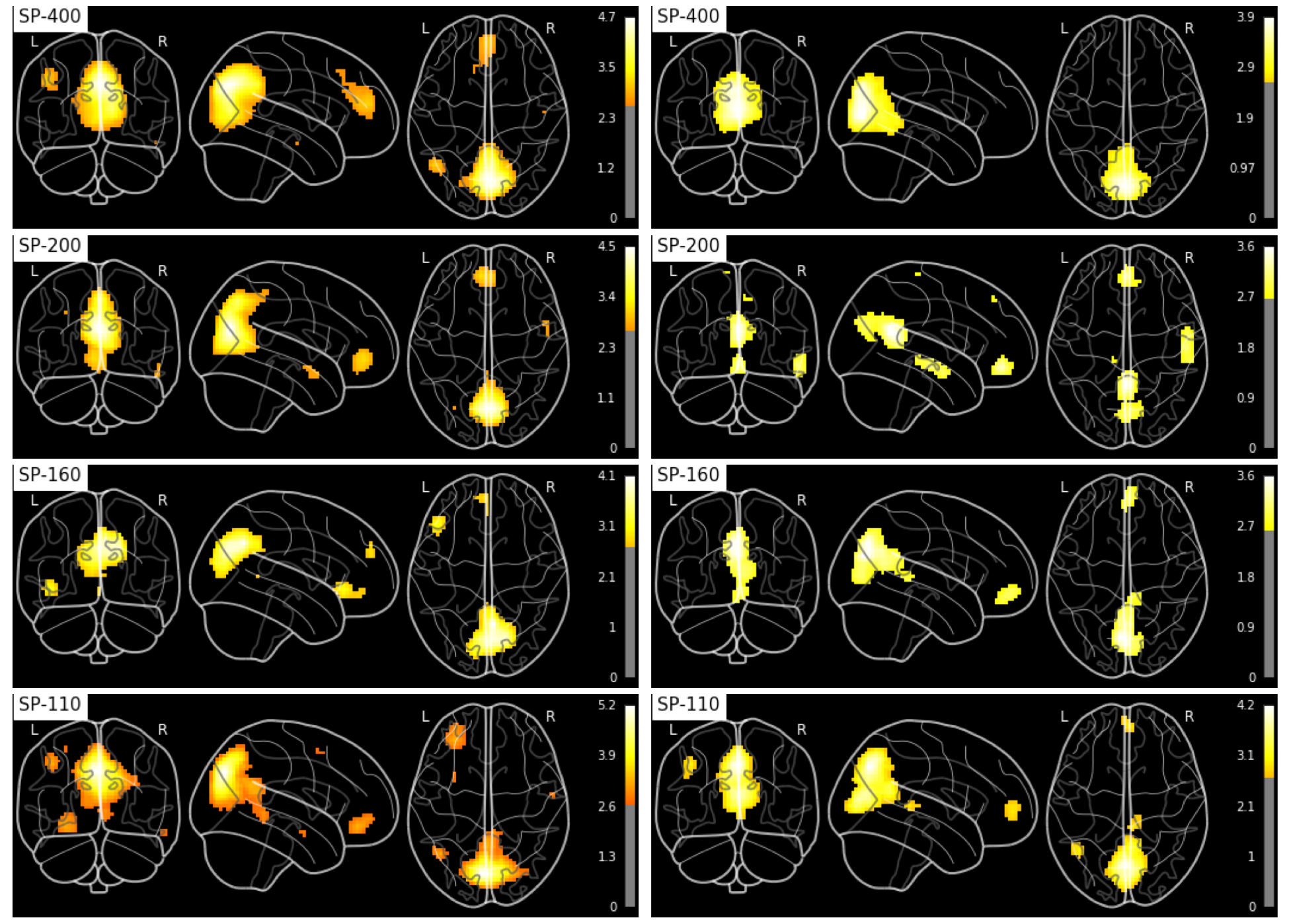
Figure S.2: Saliency maps of trained CNN models for 2 randomly chosen stochastic parcellations at each scale for ASD-HC classification.

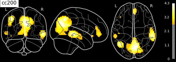
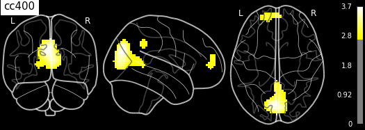
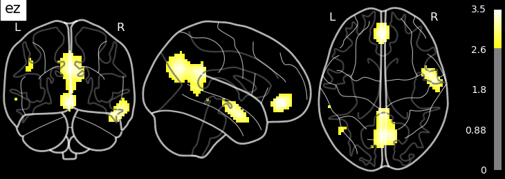
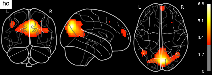
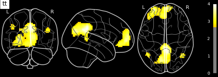
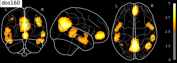
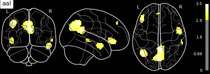
Figure S.3: Saliency maps for atlas-based ASD-HC classification models.

7.7 Comparison of different preprocessing strategies

Since preprocessing options such as nuisance regression have been a point of contention in several studies, we conducted another set of experiments with standard atlas masks in three preprocessing scenarios (a) without global signal regression(GSR) + with CompCor (b) without GSR + without CompCor and (c) with GSR + without CompCor. Below, we include the results obtained with models trained on the ABIDE-1 data using the hyperparameters optimized in our original experiments presented in the paper. The accuracy values were computed based on test predictions on the independent ABIDE-2 dataset, following our original evaluation protocol. As can be seen from Tables  S.4 and S.5, when neither GSR nor CompCor is employed during preprocessing, the prediction performance on both the tasks, i.e., ASD/HC Classification and age prediction, drops significantly. However, similar performance is obtained when using either or both of CompCor and GSR in preprocessing. Importantly, the trend remains the same: the 3D-CNN fares favorably against the baseline algorithms and the MA-Ensemble models generally perform better than or similar to the best-performing atlas.

Table S.4: Classification accuracy for ASD vs. Control: Independent results on ABIDE-II for benchmark models and proposed CNN approach. Green indicates better performance, whereas orange/red highlights worse performance.

Table S.5: Root mean squared error (RMSE in years) for age prediction: Independent results on ABIDE-II for benchmark models and proposed CNN approach. Green indicates better performance, whereas orange/red highlights worse performance.

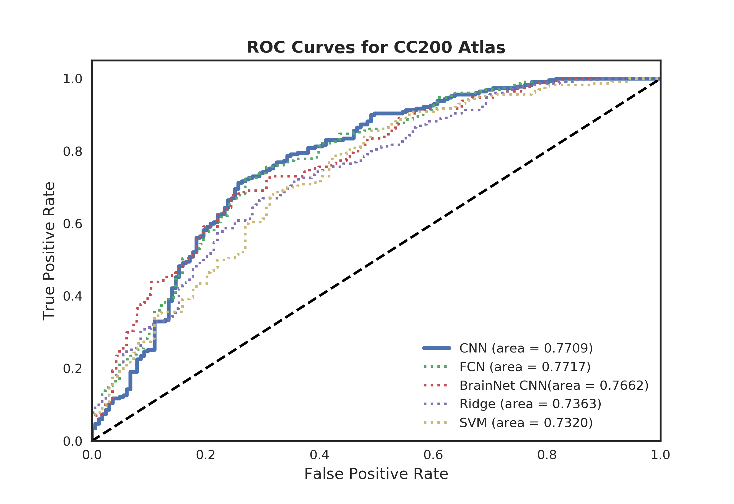
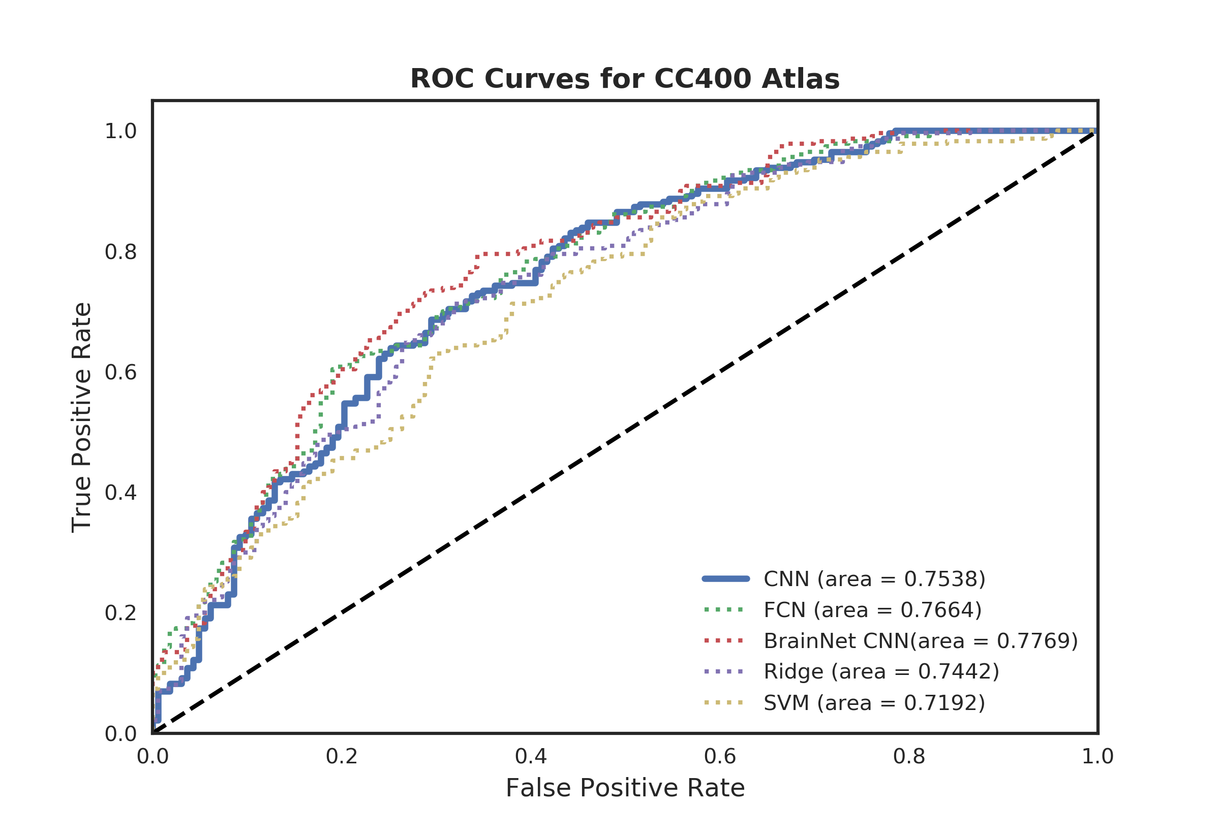
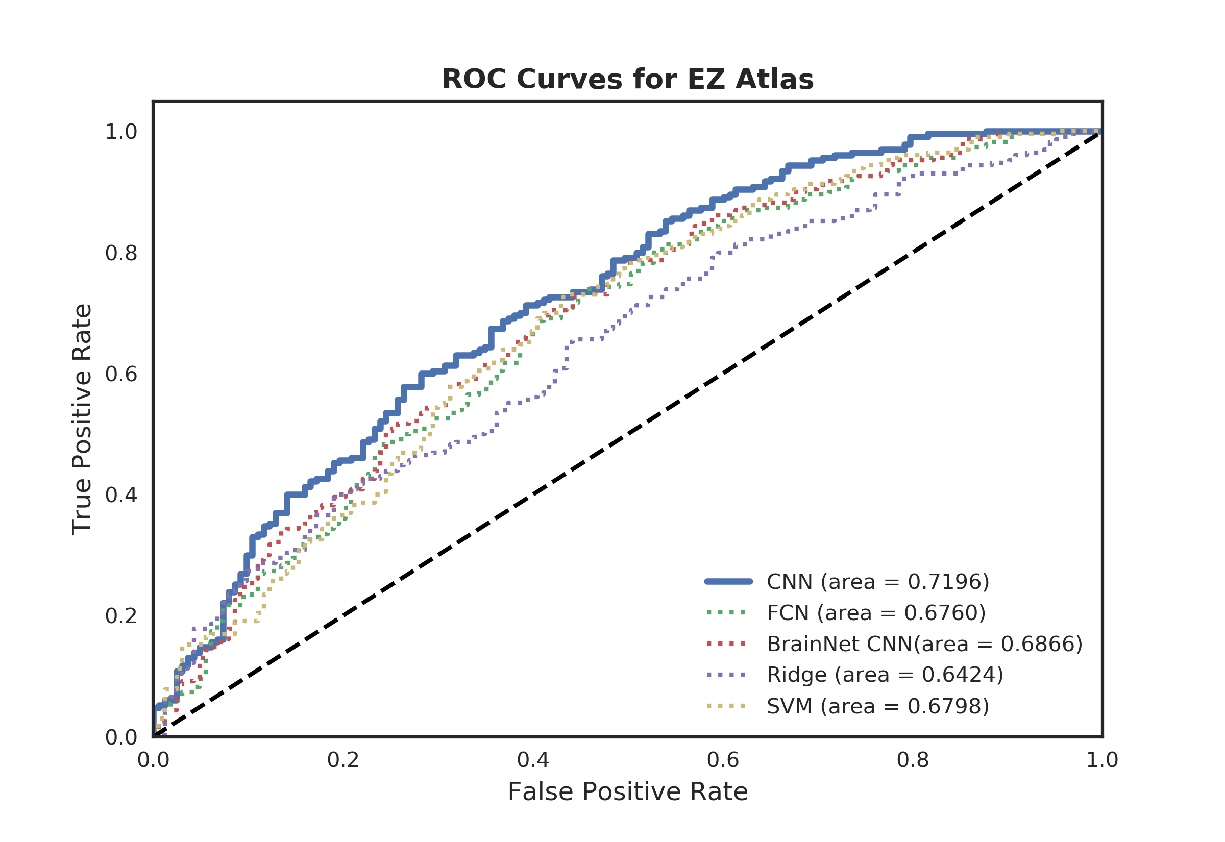
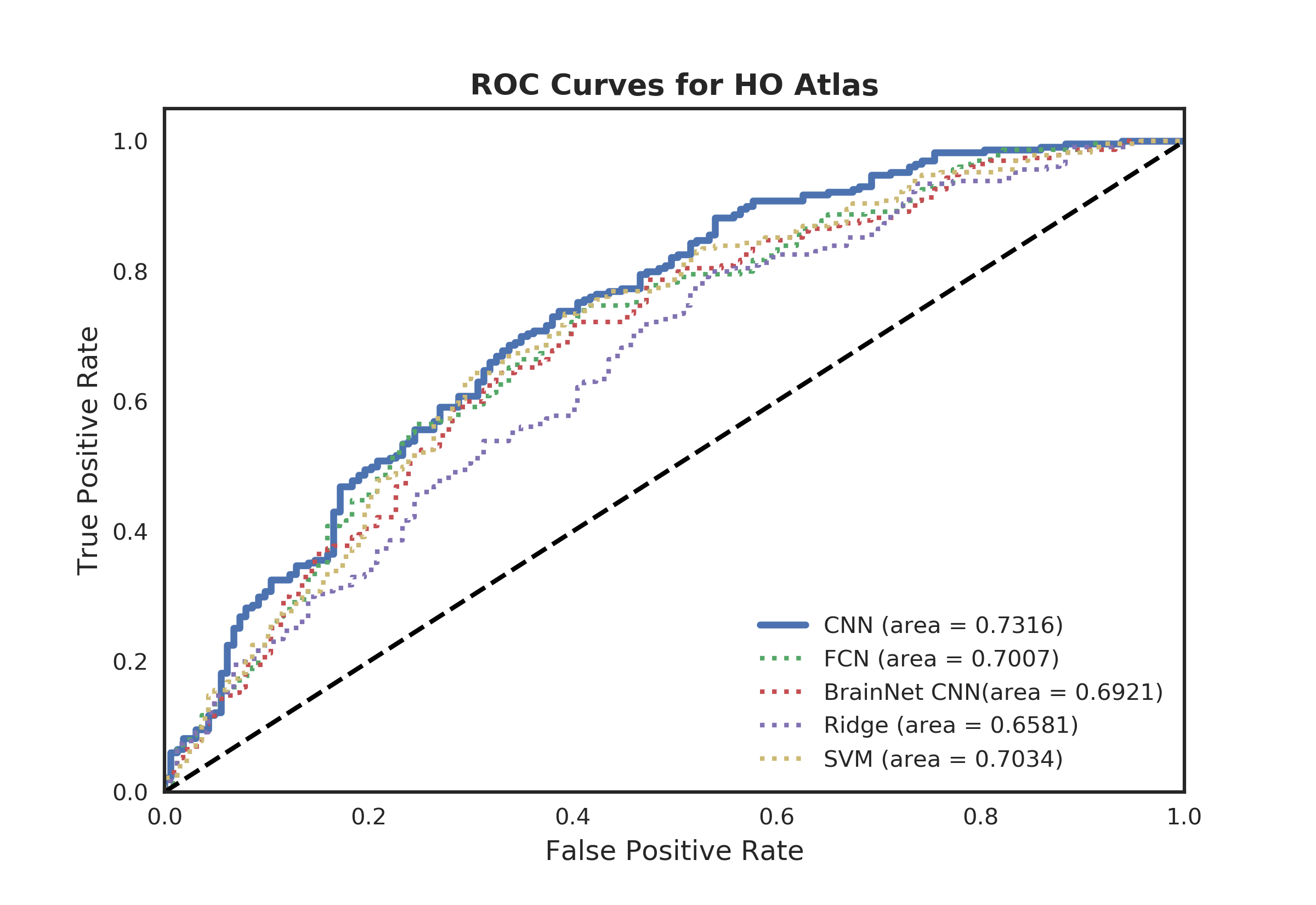
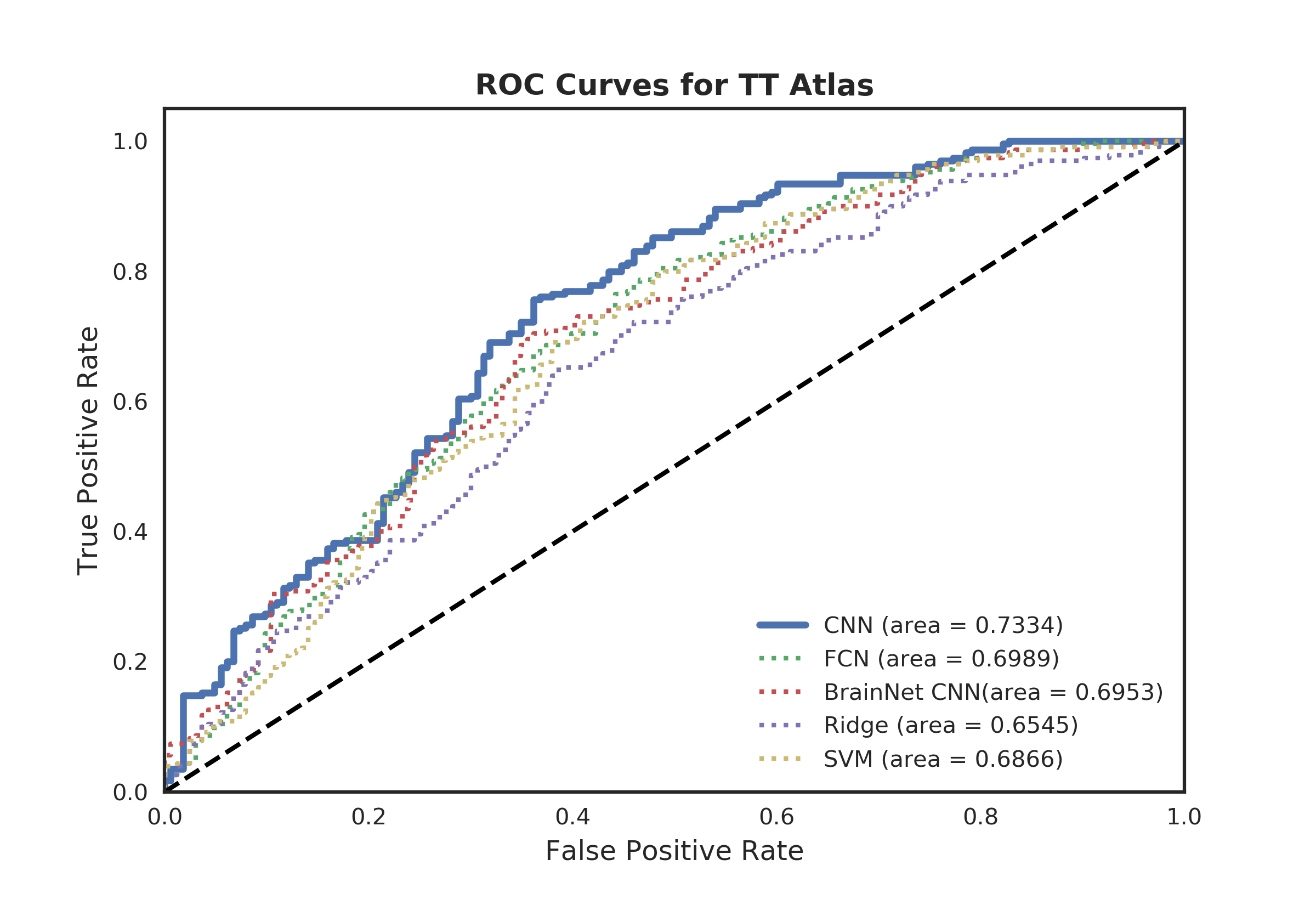
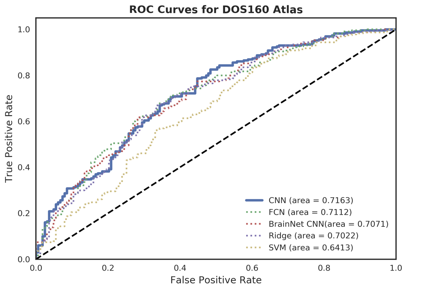
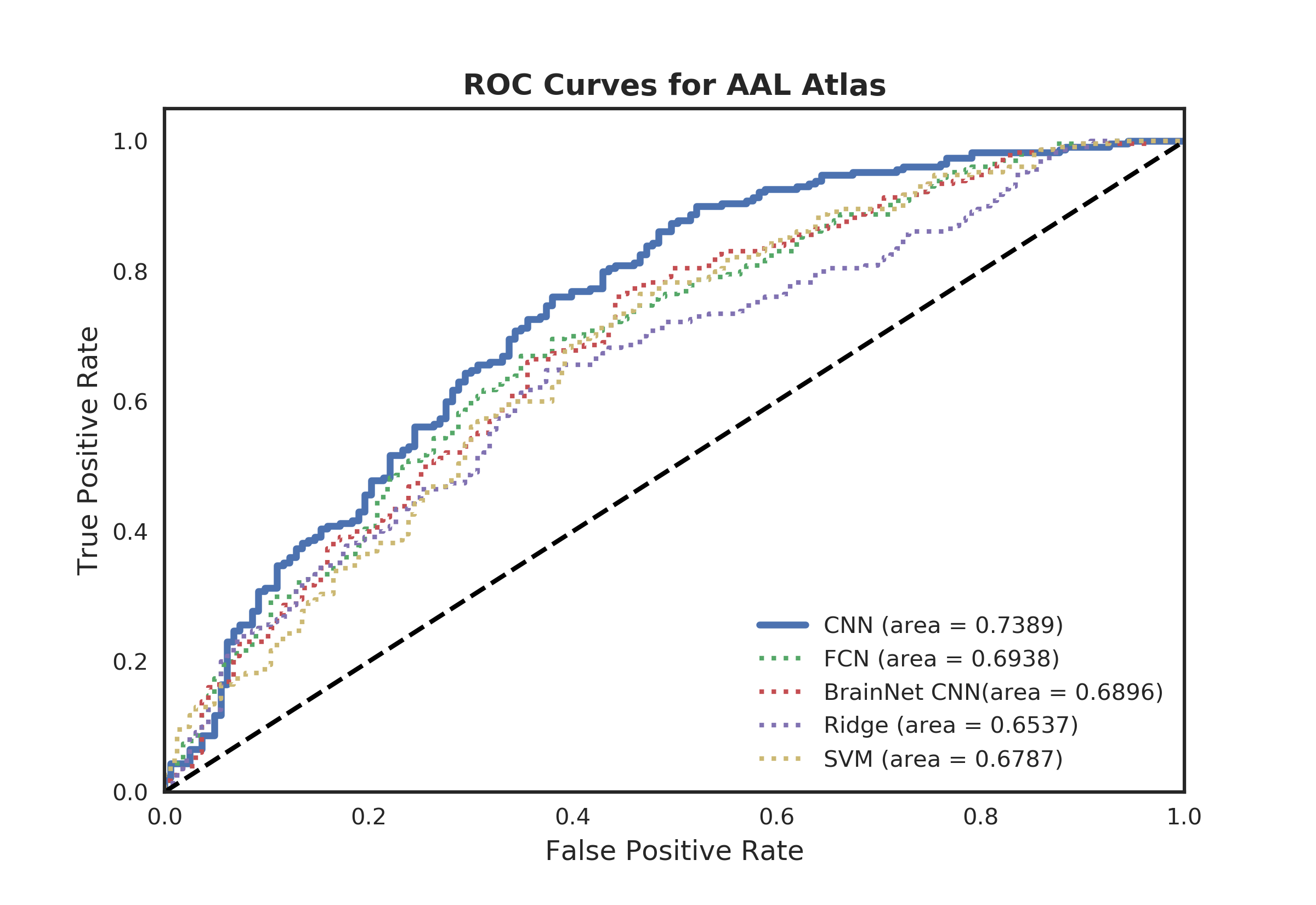
Figure S.4: ROC Curves for individual atlas based ASD-HC classification models.

Table S.6: Mean absolute error (MAE in years) for age prediction: Independent testing on ABIDE-II for benchmark models and proposed CNN approach. For each row, best results are bolded. For each column, best results are italicized. Green indicates better performance, whereas orange/red highlights worse performance.

References

- Plitt et al. [2015] M. Plitt, K. A. Barnes, A. Martin, Functional connectivity classification of autism identifies highly predictive brain features but falls short of biomarker standards, Neuroimage Clin 7 (2015) 359–366.
- Mennes et al. [2011] M. Mennes, N. Vega Potler, C. Kelly, A. Di Martino, F. X. Castellanos, M. P. Milham, Resting state functional connectivity correlates of inhibitory control in children with attention-deficit/hyperactivity disorder, Front Psychiatry 2 (2011) 83.
- Varoquaux et al. [2010] G. Varoquaux, F. Baronnet, A. Kleinschmidt, P. Fillard, B. Thirion, Detection of brain functional-connectivity difference in post-stroke patients using group-level covariance modeling, Med Image Comput Comput Assist Interv 13 (2010) 200–208.
- Brown and Hamarneh [2016] C. J. Brown, G. Hamarneh, Machine learning on human connectome data from MRI, CoRR 1611.08699 (2016).
- Kaiser [2011] M. Kaiser, A Tutorial in Connectome Analysis: Topological and Spatial Features of Brain Networks, ArXiv e-prints (2011).
- Alexander-Bloch et al. [2013] A. Alexander-Bloch, P. E. Vértes, R. Stidd, F. Lalonde, L. Clasen, J. L. Rapoport, J. N. Giedd, E. T. Bullmore, N. Gogtay, The anatomical distance of functional connections predicts brain network topology in health and schizophrenia., Cerebral cortex 23 1 (2013) 127–38.
- Smith et al. [2011] S. M. Smith, K. L. Miller, G. Salimi-Khorshidi, M. Webster, C. F. Beckmann, T. E. Nichols, J. D. Ramsey, M. W. Woolrich, Network modelling methods for FMRI (2011).
- Yao et al. [2015] Z. Yao, B. Hu, Y. Xie, P. Moore, J. Zheng, A review of structural and functional brain networks: small world and atlas, Brain Informatics 2 (2015) 45–52.
- Dadi et al. [2018] K. Dadi, M. Rahim, A. Abraham, D. Chyzhyk, M. Milham, B. Thirion, G. Varoquaux, Benchmarking functional connectome-based predictive models for resting-state fMRI, 2018. Working paper or preprint.
- Fischl et al. [2002] B. Fischl, D. H. Salat, E. Busa, M. Albert, M. Dieterich, C. Haselgrove, A. Van Der Kouwe, R. Killiany, D. Kennedy, S. Klaveness, et al., Whole brain segmentation: automated labeling of neuroanatomical structures in the human brain, Neuron 33 (2002) 341–355.
- Glasser et al. [2016] M. F. Glasser, T. S. Coalson, E. C. Robinson, C. D. Hacker, J. Harwell, E. Yacoub, K. Ugurbil, J. Andersson, C. F. Beckmann, M. Jenkinson, et al., A multi-modal parcellation of human cerebral cortex, Nature 536 (2016) 171–178.
- Eickhoff et al. [2015] S. B. Eickhoff, B. Thirion, G. Varoquaux, D. Bzdok, Connectivity-based parcellation: Critique and implications, Human brain mapping 36 (2015) 4771–4792.
- Arslan et al. [2018] S. Arslan, S. I. Ktena, A. Makropoulos, E. C. Robinson, D. Rueckert, S. Parisot, Human brain mapping: A systematic comparison of parcellation methods for the human cerebral cortex, NeuroImage 170 (2018) 5 – 30. Segmenting the Brain.
- Yushkevich et al. [2015] P. A. Yushkevich, R. S. Amaral, J. C. Augustinack, A. R. Bender, J. D. Bernstein, M. Boccardi, M. Bocchetta, A. C. Burggren, V. A. Carr, M. M. Chakravarty, et al., Quantitative comparison of 21 protocols for labeling hippocampal subfields and parahippocampal subregions in in vivo mri: towards a harmonized segmentation protocol, Neuroimage 111 (2015) 526–541.
- Varoquaux et al. [2011] G. Varoquaux, A. Gramfort, F. Pedregosa, V. Michel, B. Thirion, Multi-subject dictionary learning to segment an atlas of brain spontaneous activity, in: Biennial International Conference on Information Processing in Medical Imaging, Springer, pp. 562–573.
- Thomas Yeo et al. [2011] B. T. Thomas Yeo, F. M. Krienen, J. Sepulcre, M. R. Sabuncu, D. Lashkari, M. Hollinshead, J. L. Roffman, J. W. Smoller, L. Zöllei, J. R. Polimeni, B. Fischl, H. Liu, R. L. Buckner, The organization of the human cerebral cortex estimated by intrinsic functional connectivity, Journal of Neurophysiology 106 (2011) 1125–1165. PMID: 21653723.
- Thirion et al. [2014] B. Thirion, G. Varoquaux, E. Dohmatob, J.-B. Poline, Which fmri clustering gives good brain parcellations?, Frontiers in neuroscience 8 (2014) 167.
- Abraham et al. [2017] A. Abraham, M. P. Milham, A. D. Martino, R. C. Craddock, D. Samaras, B. Thirion, G. Varoquaux, Deriving reproducible biomarkers from multi-site resting-state data: An autism-based example, NeuroImage 147 (2017) 736 – 745.
- Ktena et al. [2018] S. I. Ktena, S. Parisot, E. Ferrante, M. Rajchl, M. Lee, B. Glocker, D. Rueckert, Metric learning with spectral graph convolutions on brain connectivity networks, NeuroImage 169 (2018) 431 – 442.
- Kawahara et al. [2016] J. Kawahara, C. Brown, S. P Miller, B. Booth, V. Chau, R. Grunau, J. Zwicker, G. Hamarneh, Brainnetcnn: Convolutional neural networks for brain networks; towards predicting neurodevelopment 146 (2016).
- Cherkassky et al. [2006] V. L. Cherkassky, R. K. Kana, T. A. Keller, M. A. Just, Functional connectivity in a baseline resting-state network in autism., Neuroreport 17 16 (2006) 1687–90.
- Assaf et al. [2010] M. Assaf, K. Jagannathan, V. Calhoun, L. Miller, M. Stevens, R. Sahl, J. O’Boyle, R. Schultz, G. Pearlson, Abnormal functional connectivity of default mode sub-networks in autism spectrum disorder patients 53 (2010) 247–56.
- Monk et al. [2009] C. S. Monk, S. J. Peltier, J. L. Wiggins, S.-J. Weng, M. Carrasco, S. Risi, C. Lord, Abnormalities of intrinsic functional connectivity in autism spectrum disorders,, NeuroImage 47 (2009) 764 – 772.
- Heinsfeld et al. [2018] A. S. Heinsfeld, et al., Identification of autism spectrum disorder using deep learning and the abide dataset, in: NeuroImage: Clinical.
- Yahata et al. [2016] N. Yahata, J. Morimoto, R. Hashimoto, G. Lisi, K. Shibata, K. Y, A small number of abnormal brain connections predicts adult autism spectrum disorder, Nature Communications 7 (2016).
- Di Martino et al. [2017] A. Di Martino, D. O’Connor, B. Chen, K. Alaerts, J. S. Anderson, M. Assaf, J. H. Balsters, L. Baxter, A. Beggiato, S. Bernaerts, L. M. E. Blanken, S. Y. Bookheimer, B. B. Braden, L. Byrge, F. X. Castellanos, M. Dapretto, R. Delorme, D. A. Fair, I. Fishman, J. Fitzgerald, L. Gallagher, R. J. J. Keehn, D. P. Kennedy, J. E. Lainhart, B. Luna, S. H. Mostofsky, R.-A. Müller, M. B. Nebel, J. T. Nigg, K. O’Hearn, M. Solomon, R. Toro, C. J. Vaidya, N. Wenderoth, T. White, R. C. Craddock, C. Lord, B. Leventhal, M. P. Milham, Enhancing studies of the connectome in autism using the autism brain imaging data exchange ii, Scientific data 4 (2017) 170010.
- Craddock et al. [2013] C. Craddock, Y. Benhajali, C. Chu, F. Chouinard, A. Evans, A. Jakab, B. S. Khundrakpam, J. D. Lewis, Q. Li, M. Milham, C. Yan, P. Bellec, The neuro bureau preprocessing initiative: open sharing of preprocessed neuroimaging data and derivative, Frontiers in Neuroinformatics (2013).
- Power et al. [2014] J. D. Power, A. Mitra, T. O. Laumann, A. Z. Snyder, B. L. Schlaggar, S. E. Petersen, Methods to detect, characterize, and remove motion artifact in resting state fMRI, NeuroImage 84 (2014) 320–341.
- Muschelli et al. [2014] J. Muschelli, M. B. Nebel, B. S Caffo, A. Barber, J. J Pekar, S. H Mostofsky, Reduction of motion-related artifacts in resting state fmri using acompcor 96 (2014).
- Frazier et al. [2005] J. A. Frazier, et al., Structural brain magnetic resonance imaging of limbic and thalamic volumes in pediatric bipolar disorder., The American journal of psychiatry 162 7 (2005).
- Goldstein et al. [2007] J. M. Goldstein, L. J. Seidman, N. Makris, T. Ahern, L. M. O’Brien, V. S. Caviness, D. N. Kennedy, S. V. Faraone, M. T. Tsuang, Hypothalamic abnormalities in schizophrenia: sex effects and genetic vulnerability, Biol. Psychiatry 61 (2007) 935–945.
- Makris et al. [2006] N. Makris, J. M. Goldstein, D. Kennedy, S. M. Hodge, V. S. Caviness, S. V. Faraone, M. T. Tsuang, L. J. Seidman, Decreased volume of left and total anterior insular lobule in schizophrenia, Schizophr. Res. 83 (2006) 155–171.
- Smyser et al. [2016] C. D. Smyser, N. U. Dosenbach, T. A. Smyser, A. Z. Snyder, C. E. Rogers, T. E. Inder, B. L. Schlaggar, J. J. Neil, Prediction of brain maturity in infants using machine-learning algorithms, Neuroimage 136 (2016) 1–9.
- Desikan et al. [2006] R. S. Desikan, F. Segonne, B. Fischl, B. T. Quinn, B. C. Dickerson, D. Blacker, R. L. Buckner, A. M. Dale, R. P. Maguire, B. T. Hyman, M. S. Albert, R. J. Killiany, An automated labeling system for subdividing the human cerebral cortex on MRI scans into gyral based regions of interest, Neuroimage 31 (2006) 968–980.
- Tzourio-Mazoyer et al. [2002] N. Tzourio-Mazoyer, B. Landeau, D. Papathanassiou, F. Crivello, O. Etard, N. Delcroix, B. Mazoyer, M. Joliot, Automated anatomical labeling of activations in SPM using a macroscopic anatomical parcellation of the MNI MRI single-subject brain, Neuroimage 15 (2002) 273–289.
- Cameron et al. [2011] C. Cameron, G. James, P. Holtzheimer, X. Hu, M. HS., A whole brain fmri atlas generated via spatially constrained spectral clustering, Human Brain Mapping 33 (2011) 1914–1928.
- Lancaster et al. [2000] J. L. Lancaster, M. G. Woldorff, L. M. Parsons, M. Liotti, C. S. Freitas, L. Rainey, P. V. Kochunov, D. Nickerson, S. A. Mikiten, P. T. Fox, Automated talairach atlas labels for functional brain mapping, Human Brain Mapping 10 (2000) 120–131.
- Eickhoff et al. [2005] S. B. Eickhoff, K. E. Stephan, H. Mohlberg, C. Grefkes, G. R. Fink, K. Amunts, K. Zilles, A new SPM toolbox for combining probabilistic cytoarchitectonic maps and functional imaging data, Neuroimage 25 (2005) 1325–1335.
- Schirmer [2015] M. D. Schirmer, Developing Brain Connectivity - Effects of Parcellation Scale on Network Analysis in Neonates (Doctoral dissertation, King’s College London) (2015).
- Ioffe and Szegedy [2015] S. Ioffe, C. Szegedy, Batch normalization: Accelerating deep network training by reducing internal covariate shift, CoRR abs/1502.03167 (2015).
- Simonyan et al. [2013] K. Simonyan, A. Vedaldi, A. Zisserman, Deep Inside Convolutional Networks: Visualising Image Classification Models and Saliency Maps, ArXiv e-prints (2013).
- Utevsky et al. [2014] A. V. Utevsky, D. V. Smith, S. A. Huettel, Precuneus is a functional core of the default-mode network, Journal of Neuroscience 34 (2014) 932–940.
- Watanabe et al. [2012] T. Watanabe, N. Yahata, O. Abe, H. Kuwabara, H. Inoue, Y. Takano, N. Iwashiro, T. Natsubori, Y. Aoki, H. Takao, et al., Diminished medial prefrontal activity behind autistic social judgments of incongruent information, PloS one 7 (2012) e39561.
- Koshino et al. [2005] H. Koshino, P. A. Carpenter, N. J. Minshew, V. L. Cherkassky, T. A. Keller, M. A. Just, Functional connectivity in an fmri working memory task in high-functioning autism, Neuroimage 24 (2005) 810–821.
- Reuter-Lorenz et al. [2000] P. A. Reuter-Lorenz, J. Jonides, E. E. Smith, A. Hartley, A. Miller, C. Marshuetz, R. A. Koeppe, Age differences in the frontal lateralization of verbal and spatial working memory revealed by pet, Journal of cognitive neuroscience 12 (2000) 174–187.
- Craddock et al. [2012] R. C. Craddock, G. James, P. E. Holtzheimer, X. P. Hu, H. S. Mayberg, A whole brain fMRI atlas generated via spatially constrained spectral clustering, Human Brain Mapping 33 (2012) 1914–1928.
- Fornito et al. [2010] A. Fornito, A. Zalesky, E. T. Bullmore, Network scaling effects in graph analytic studies of human resting-state FMRI data, Front Syst Neurosci 4 (2010) 22.
- Zalesky et al. [2010] A. Zalesky, A. Fornito, I. H. Harding, L. Cocchi, M. Yucel, C. Pantelis, E. T. Bullmore, Whole-brain anatomical networks: does the choice of nodes matter?, Neuroimage 50 (2010) 970–983.
- Kong et al. [2018] R. Kong, J. Li, C. Orban, M. R. Sabuncu, H. Liu, A. Schaefer, N. Sun, X. N. Zuo, A. J. Holmes, S. B. Eickhoff, B. T. T. Yeo, Spatial Topography of Individual-Specific Cortical Networks Predicts Human Cognition, Personality, and Emotion, Cereb. Cortex (2018).
- Da Mota et al. [????] B. Da Mota, V. Fritsch, G. Varoquaux, V. Frouin, J. Poline, T. B., Enhancing the reproducibility of group analysis with randomized brain parcellations, in: Medical Image Computing and Computer-Assisted Intervention - MICCAI 2013. Lecture Notes in Computer Science, vol 8150. Springer, Berlin, Heidelberg.
- Chen et al. [2015] C. P. Chen, C. L. Keown, A. Jahedi, A. Nair, M. E. Pflieger, B. A. Bailey, R. A. Muller, Diagnostic classification of intrinsic functional connectivity highlights somatosensory, default mode, and visual regions in autism, Neuroimage Clin 8 (2015) 238–245.
- Menon [2013] V. Menon, Developmental pathways to functional brain networks: emerging principles, Trends Cogn. Sci. (Regul. Ed.) 17 (2013) 627–640.
- Satterthwaite et al. [2012] T. D. Satterthwaite, D. H. Wolf, J. Loughead, K. Ruparel, M. A. Elliott, H. Hakonarson, R. C. Gur, R. E. Gur, Impact of in-scanner head motion on multiple measures of functional connectivity: Relevance for studies of neurodevelopment in youth, NeuroImage 60 (2012) 623 – 632.
- Fair et al. [2013] D. Fair, J. Nigg, S. Iyer, D. Bathula, K. Mills, N. Dosenbach, B. Schlaggar, M. Mennes, D. Gutman, S. Bangaru, J. Buitelaar, D. Dickstein, A. Di Martino, D. Kennedy, C. Kelly, B. Luna, J. Schweitzer, K. Velanova, Y.-F. Wang, S. Mostofsky, F. Castellanos, M. Milham, Distinct neural signatures detected for adhd subtypes after controlling for micro-movements in resting state functional connectivity mri data, Frontiers in Systems Neuroscience 6 (2013) 80.
- Van Dijk et al. [2012] K. R. Van Dijk, M. R. Sabuncu, R. L. Buckner, The influence of head motion on intrinsic functional connectivity mri, Neuroimage 59 (2012) 431–438.
- Hagmann et al. [2008] P. Hagmann, L. Cammoun, X. Gigandet, R. Meuli, C. J. Honey, V. J. Wedeen, O. Sporns, Mapping the structural core of human cerebral cortex, PLOS Biology 6 (2008) 1–15.
- Zintgraf et al. [2017] L. M. Zintgraf, T. S. Cohen, T. Adel, M. Welling, Visualizing deep neural network decisions: Prediction difference analysis, CoRR abs/1702.04595 (2017).
- Selvaraju et al. [2016] R. R. Selvaraju, A. Das, R. Vedantam, M. Cogswell, D. Parikh, D. Batra, Grad-cam: Why did you say that? visual explanations from deep networks via gradient-based localization, CoRR abs/1610.02391 (2016).
- Bridson [2007] R. Bridson, Fast poisson disk sampling in arbitrary dimensions, in: ACM SIGGRAPH 2007 Sketches, SIGGRAPH ’07, ACM, New York, NY, USA, 2007.