Periodic orbits of discrete and continuous dynamical systems via Poincaré-Miranda theorem

Abstract

We present a systematic methodology to determine and locate analytically isolated periodic points of discrete and continuous dynamical systems with algebraic nature. We apply this method to a wide range of examples, including a one-parameter family of counterexamples to the discrete Markus-Yamabe conjecture (La Salle conjecture); the study of the low periods of a Lotka-Volterra-type map; the existence of three limit cycles for a piece-wise linear planar vector field; a new counterexample of Kouchnirenko’s conjecture; and an alternative proof of the existence of a class of symmetric central configuration of the $(1+4)$-body problem.

Mathematics Subject Classification 2010: 37C25, 39A23 (Primary); 13P15, 34D23, 70F15, 70K05 (Secondary).

Keywords: Poincaré-Miranda theorem; Periodic orbits; Lotka-Volterra maps; Thue-Morse maps; Discrete Markus-Yamabe conjecture; Kouchnirenko’s conjecture; Limit cycles; Planar piecewise linear systems; Central configurations.

1 Introduction and main results

Periodic orbits are one of the main objects of study of the theory of dynamic systems. A priori there are many ways to prove the existence periodic orbits, for instance one can try to apply the plenty of available fixed point theorems [15] or results guaranteeing the existence of zeros, since periodic orbits are always solutions of equations of the form $G(\mathbf{x})=\mathbf{x}$, where $G$ is a return map in the continuous case, and $G=F^{p}$ for some $p\in{\mathbb{N}}$ in the case of a discrete system given by a map $F$. However when one tries to apply these results to a particular case it is not always easy to find effective ways to check the hypotheses. An example of this fact appears when trying to use the Newton-Kantorovich Theorem [19]. By using this approach, some bounds of the partial derivatives of the involved functions must be obtained. The work done in [3] exemplifies clearly the difficulties of this approach.

In this work we present an effective procedure to prove the existence, determine the number and locate periodic orbits of dynamical systems of both discrete and continuous nature. This procedure is explained in detail in the next sections. As we will see, one of the main features of this procedure is the use of the Poincaré-Miranda theorem (PMT for short). We believe that one of the advantages of using PMT for finding fixed points of a given function is that only the signs of the components of it have to be controlled on some suitable sets, which is straightforward in the case that either the equations are polynomial or the problem can be polynomialized (see for instance the proof of Theorem 6 in Section 5). Recall that the use of Sturm sequences for polynomials in $\mathbb{Q}[x]$ allows to control their signs on intervals with rational endpoints ([32]).

The PMT is the extension of the Bolzano theorem to higher dimensions. It was formulated and proved by H. Poincaré in 1883 and 1886 respectively, [29, 30]. C. Miranda re-obtained the result as an equivalent formulation of Brouwer fixed point theorem in 1940, [28]. Recent proofs are presented in [21, 33]. For completeness, we recall it. As usual, $\overline{S}$ and $\partial S$ denote, respectively, the closure and the boundary of a set $S\subset{\mathbb{R}}^{n}.$

Theorem 1 (Poincaré-Miranda).

Set $\mathcal{B}=\{\mathbf{x}=(x_{1},\ldots,x_{n})\in{\mathbb{R}}^{n}\,:\,L_{i}<x_{i}<U_{i},1\leq i\leq n\}$. Suppose that $f=(f_{1},f_{2},\ldots,f_{n}):\overline{\mathcal{B}}\rightarrow R^{n}$ is continuous, $f(\mathbf{x})\neq\mathbf{0}$ for all $\mathbf{x}\in\partial\mathcal{B}$, and for $1\leq i\leq n,$

$$f_{i}(x_{1},\ldots,x_{i-1},L_{i},x_{i+1},\ldots,x_{n})\leq 0\,\mbox{ and }\,f_{i}(x_{1},\ldots,x_{i-1},U_{i},x_{i+1},\ldots,x_{n})\geq 0,$$

Then, there exists $\mathbf{s}\in\mathcal{B}$ such that $f(\mathbf{s})=\mathbf{0}$.

For short, when given a map $f$ we have a box $\mathcal{B}$ such that the hypotheses of the PMT hold we will say that $\mathcal{B}$ is a PM box. When we try to apply PMT to some $f,$ sometimes it is better to consider some permutation of its components.

The paper is structured as follows: we start giving a new degree 6 counterexample of Kouchnirenko conjecture to illustrate the use and utility of our approach. In Section 3, we prove the existence of a 1-parameter family of rational counterexamples to a conjecture of La Salle (also known as discrete Markus-Yamabe conjecture) that extends the results of [6] providing also an alternative proof of them. In Section 4 we prove the existence of exactly two $5$-periodic orbits and three $6$-periodic orbits in a certain region for a Lotka-Volterra-type map correcting and complementing some results that appear in the literature. In Section 5 we provide another example of planar piecewise linear differential system with two zones having $3$-limit cycles. Finally, in Section 6 we use PMT to give an alternative proof of the existence of a type of symmetric central configuration of the $(1+4)$-body problem.

2 A new counterexample to Kouchnirenko conjecture

Descartes’ rule asserts that a 1-variable real polynomial with $m$ monomials has at most $m-1$ simple positive real roots. The Kouchnirenko conjecture was posed as an attempt to extend this rule to the several variables context. In the 2-variables case this conjecture said that a real polynomial system $f_{1}(x,y)=f_{2}(x,y)=0$ would have at most $(m_{1}-1)(m_{2}-1)$ simple solutions with positive coordinates, where $m_{i}$ is the number of monomials of each $f_{i}$. This conjecture was stated by A. Kouchnirenko in the late 70’s, and published in the A. G. Khovanskiĭ’s paper [20]. In 2000, B. Haas ([17]) constructed a family of counterexamples given by two trimonomials, being the minimal degree of these counterexamples 106. In 2007 a much simpler family of counterexamples was presented in [9], being the simplest one again formed by two trimonomials, but of degree $6.$ Both examples have exactly $5$ simple solutions with positive coordinates instead of the $4$ predicted by the conjecture. In 2003, it was proved in [23] that any pair of bivariate trinomials has at most 5 simple solutions.

We will prove in a very simple way, by using PMT, that system

$$\left\{\begin{array}[]{l}P(x,y):=x^{6}+ay^{3}-y=0,\\ Q(x,y):=y^{6}+ax^{3}-x=0,\end{array}\right.$$

with $a=61/43\simeq 1.41860465$ is a counterexample of the conjecture. We remark that in [9] it was given the counterexample with $a=44/31.$ The reason why we have changed this parameter is that it can be proved that when $a=\overline{a}=7\times 12^{4/5}/36\simeq 1.14195168$ the above system has the multiple solution $(s,s)$ with $s=12^{3/5}/6\simeq 0.74021434$ and $\overline{a}$ is quite close to $44/31\simeq 1.4193548,$ making that, for that system, 3 of the its 5 solutions with positive entries are very close to each other. By using the approach developed in [12, 13], or the tools of [9], it can be proved that counterexamples to the conjecture only appear for $a\in(\underline{a},\overline{a}),$ where $\underline{a}\simeq 1.4176595.$ Both values are zeroes of some irreducible factor of the polynomial $\Delta_{y}(\mathrm{Res}(P,Q;x)),$ where $\Delta_{y}$ and $\mathrm{Res}$ denote, as usual, the discriminant and the resultant respectively. Hence, our value of $a$ has also small numerator and denominator and, moreover, it is near the middle point of this interval, making that in the computations of our proof the rational numbers involved are simpler that the ones needed to use our approach when $a=44/31.$ We prove:

Proposition 2.

The bivariate trinomial system

$$\left\{\begin{array}[]{l}P(x,y)=x^{6}+\frac{61}{43}y^{3}-y=0,\\ Q(x,y)=y^{6}+\frac{61}{43}x^{3}-x=0,\end{array}\right.$$ (1)

has 5 real simple solutions with positive entries.

Proof.

It is not difficult to find numerically 5 approximated solutions of the system. They are $(\widetilde{x}_{1},\widetilde{x}_{5})$, $(\widetilde{x}_{2},\widetilde{x}_{4})$, $(\widetilde{x}_{3},\widetilde{x}_{3})$, $(\widetilde{x}_{4},\widetilde{x}_{2})$, $(\widetilde{x}_{5},\widetilde{x}_{1})$, where $\widetilde{x}_{1}=0.59679166,$ $\widetilde{x}_{2}=0.68913517,$ $\widetilde{x}_{3}=0.74035310,$ $\widetilde{x}_{4}=0.77980435$ and $\widetilde{x}_{5}=0.81602099.$ We consider the following 5 intervals, with $\widetilde{x}_{i}\in I_{i},$

$$I_{1} =\left[{\frac{1}{2}},{\frac{1619}{2500}}\right],\,I_{2}=\left[{\frac{1619}{2500}},{\frac{18}{25}}\right],\,I_{3}=\left[{\frac{18}{25}},{\frac{75857}{100000}}\right],$$

$$I_{4} =\left[{\frac{75857}{100000}},{\frac{4}{5}}\right],\,I_{5}=\left[{\frac{4}{5}},{\frac{83}{100}}\right].$$

Let us prove that system (1) has 5 actual solutions $(x_{1},x_{5})$, $(x_{2},x_{4})$, $(x_{3},x_{3})$, $(x_{4},x_{2})$, $(x_{5},x_{1})$, with $x_{i}\in I_{i}.$ Firstly, since $P(x,x)=Q(x,x)=x^{6}+{61}x^{3}/43-x,$ by Descartes rule we know that there is exactly one simple positive real root of $P(x,x).$ By Bolzano theorem it belongs to $I_{3}.$ So there is a solution $(x_{3},x_{3})$ of the system in $I_{3}\times I_{3}$.

By the symmetry of the system, if $(x^{*},y^{*})$ is one of its solutions then $(y^{*},x^{*})$ also is. Hence, we only need to prove that there are two suitable different solutions. This will be proved by applying the PMT to the boxes $I_{1}\times I_{5},$ and $I_{2}\times I_{4},$ which are depicted in Figure 1.

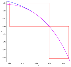
Figure 1: Intersection of the curves $P(x,y)=0$ (in blue) and $Q(x,y)=0$ (in magenta). The PM boxes $I_{1}\times I_{5}$, $I_{2}\times I_{4}$ (left and right respectively, in red).

We start applying the PMT to the box $I_{1}\times I_{5}.$ Consider the polynomials

$$P\left(\frac{1}{2},y\right)=\frac{61}{43}\,{y}^{3}-y+\frac{1}{2^{6}}\quad\mbox{and}\quad P\left(\frac{1619}{2500},y\right)=\frac{61}{43}\,{y}^{3}-y+\left(\frac{1619}{2500}\right)^{6}.$$

By computing their corresponding Sturm sequences we get that both have no roots in $[4/5,83/100].$ Moreover $P(1/2,y)<0$ and $P({1619}/{2500},y)>0$ on this interval. Similarly we get that

$$Q\left(x,\frac{4}{5}\right)={\frac{61}{43}}\,{x}^{3}-x+\left(\frac{4}{5}\right)^{6}<0\quad\mbox{and}\quad Q\left(x,\frac{83}{100}\right)={\frac{61}{43}}\,{x}^{3}-x+\left(\frac{83}{100}\right)^{6}>0$$

on $[1/2,{1619}/{2500}]$. Hence, $I_{1}\times I_{5}$ is under the hypotheses of the PMT, and system (1) has a solution $(x_{1},x_{5})$ in this box.

By using the same arguments one gets that the box $I_{2}\times I_{4},$ contains another solution $(x_{2},x_{4})$ of our system. In this case the polynomials involved are even simpler. In this occasion, for $y\in[75857/100000,4/5]$ it holds that

$$Q\left(\frac{1619}{2500},y\right)=y^{6}-\frac{176243010801}{671875\times 10^{6}}<0\quad\mbox{and}\quad Q\left(\frac{18}{25},y\right)=y^{6}-\frac{127998}{671875}>0,$$

and for $x\in[1619/2500,18/25],$ that

$$P\left(x,\frac{75857}{10^{5}}\right)=x^{6}-\frac{5991841917684627}{43\times 10^{15}}<0\,\,\mbox{and}\,\,P\left(x,\frac{4}{5}\right)=x^{6}-\frac{810993}{43\times 10^{6}}>0.$$

The above facts prove that in the boxes $I_{1}\times I_{5}$, $I_{2}\times I_{4}$ and their symmetric ones, $I_{5}\times I_{1}$ and $I_{4}\times I_{2}$, there are at least $4$ solutions of the studied system. These solutions together with the solution in the diagonal give the $5$ announced solutions with positive coordinates. To prove they are simple solutions we first compute

$$J(x,y):=\det{\rm D}(P,Q)=36{x}^{5}{y}^{5}-{\frac{33489}{1849}}{x}^{2}{y}^{2}+{\frac{183}{43}}{x}^{2}+{\frac{183}{43}}{y}^{2}-1.$$

Since $\mathrm{Res}(\mathrm{Res}(P,Q;x),\mathrm{Res}(P,J;x);y)\neq 0$, $J$ does not vanish on the solutions (real or complex) of system (1). Hence all their solutions are simple. In fact, by using that a bivariate trinomial system hay at most five different solutions ([23]) or the tools of the so-called discard procedure, that we will introduce in Section 4 we get that 5 is the exact number of solutions with positive entries and that these solutions together with $(0,0)$ are the only real solutions of the system.    

3 A counterexample to the discrete Markus-Yamabe conjecture revisited

In [22], J. P. La Salle proposed some possible sufficient conditions for discrete dynamical systems with a fixed point, $x_{n+1}=F(x_{n}),\,x\in\mathbb{R}^{n},$ to be globally asymptotically stable (GAS). One of these conditions is:

$$\mbox{ For all }x\in\mathbb{R}^{n},\,\rho\left(\mathrm{D}F(x)\right)<1,$$ (2)

where $\rho$ is the spectral radius of the differential matrix. This condition is known as a discrete Markus-Yamabe-type condition because of its similarity with the conditions of Markus-Yamabe conjecture for ordinary differential equations, stated by L. Markus and H. Yamabe in 1960 [27], that has been proved to be true in dimension two and false in superior dimensions, see for instance [7, 16].

In [6] the authors consider rational maps of the form

$$F(x,y)=\left(y,-bx+\frac{a}{(1+y^{2})^{2}}\right),$$ (3)

and prove that there exist some real values, $a=a^{*}$ and $b=b^{*},$ such that the map (3) satisfies the Markus-Yamabe condition (2) and it has the 3-periodic point $(-0.1,0.25).$ Moreover they show numerically that for $a^{*}=1.8$ and $b^{*}=0.9$ a $3$-periodic orbit seems to exist. This example was proposed to simplify the previous one given by W. Szlenk, see [5, Appendix]; and to show that even for systems coming from rational difference equations the discrete Markus-Yamabe conjecture does not hold.

In this section we apply the PMT to give a simple proof of the following result, that in particular fixes the numerical counterexample presented in [6].

Proposition 3.

For $b\in\mathbf{B}:=[113/128,2916/3125]\simeq[0.883,0.933]$ the map

$$F(x,y;b)=\left(y,-bx+\frac{2b}{(1+y^{2})^{2}}\right),$$

satisfies the Markus-Yamabe condition (2) and has a $3$-periodic orbit.

Prior to prove this proposition, we recall the following auxiliary lemma, that is a simplified version of a result given in [12].

Lemma 4.

Let $G(x;b)=g_{n}(b)x^{n}+g_{n-1}(b)x^{n-1}+\cdots+g_{1}(b)x+g_{0}(b)$ be a family of real polynomials that depend continuously on one real parameter $b\in\mathbf{B}=[b_{1},b_{2}]\subset\mathbb{R}$. Fix $J=[\underline{x},\overline{x}]\subset{\mathbb{R}}$ and assume that:

1. There exists $b_{0}\in\mathbf{B}$ such that $G(x;b_{0})$ has no real roots in $J$.

2. For all $b\in\mathbf{B}$, $G(\underline{x};b)\cdot G(\overline{x};b)\cdot\Delta_{x}(G_{b})\neq 0,$ where $\Delta_{x}(G(\cdot;b))$ is the discriminant of $G(x;b)$ with respect to $x.$

Then for all $b\in\mathbf{B}$, $G(x;b)$ has no real roots in $J$.

Proof of Proposition 3.

We start noticing that in [6], it is proved that the maps (3) satisfy condition (2) if and only if $|a|<\sqrt{{11664}/{3125}}$ and $b\in({3125a^{2}}/{11664},1).$ When $a=2b$ these conditions reduce to $b\in\left(0,{2916}/{3125}\right).$

The 3-periodic points are solutions of system $F^{2}(x,y;b)=F^{-1}(x,y;b)$, that can be studied trough the equivalent system

$$g_{i}(x,y;b):=\operatorname{Numer}\left(F^{2}_{i}(x,y;b)-F^{-1}_{i}(x,y)\right)=0,\quad i=1,2,$$ (4)

where, as usual, $G_{i}$ denotes the $i$-th component of a map $G$. Some computations give

$$g_{1}(x,y;b)=\!\!-{b}^{2}{x}^{5}{y}^{4}-2{b}^{2}{x}^{5}{y}^{2}-2{b}^{2}{x}^{3}{y}^{4}+{x}^{4}{y}^{5}-{b}^{2}{x}^{5}-4{b}^{2}{x}^{3}{y}^{2}-{b}^{2}x{y}^{4}+2{x}^{4}{y}^{3}$$

$$+2{x}^{2}{y}^{5}+2{b}^{2}{x}^{4}-2{b}^{2}{x}^{3}-2{b}^{2}x{y}^{2}-2b{y}^{4}+{x}^{4}y+4{x}^{2}{y}^{3}+{y}^{5}+4{b}^{2}{x}^{2}-{b}^{2}x-4b{y}^{2}$$

$$+2{x}^{2}y+2{y}^{3}+2{b}^{2}-2b+y$$

and that $g_{2}(x,y;b)$ has degree 21 in $(x,y)$ and degree $5$ in $b.$ We omit its expression.

We claim, now, that for any $b\in(\underline{b},\overline{b})=(113/128,123/128)\simeq(0.883,0.961)$ there is a solution of system (4) in the box $\mathcal{B}:=\left[-0.2,0\right]\times\left[0,0.5\right]$, corresponding with a $3$-periodic point, where this interval of values of $b$ is not optimal. Notice that the box $\mathcal{B}$ does not contain points on the diagonal line $y=x$ and so, the found solution is not a fixed point, but a $3$-periodic one. The curves $g_{1}(x,y;0.9)=0$ (in blue) and $g_{2}(x,y;0.9)=0$ (in magenta), together with the box $\mathcal{B},$ are depicted in Figure 2.

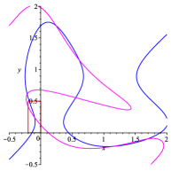
Figure 2: Intersection the curves $g_{1}(x,y;0.9)=0$ (in blue) and $g_{2}(x,y;0.9)=0$ (in magenta). It can be seen that there are seven intersection corresponding to one fixed point and two different $3$-periodic orbits. In red, a PM box of one of the solutions of system (4).

In consequence, for $b\in\mathbf{B}$ the map satisfies the Markus-Yamabe condition (2) and has a $3$-periodic point, as we wanted to prove. The claim will follow from PMT applied to the map $f=(g_{1},g_{2})$, once we prove for all $b\in\mathbf{B}$:

1. $h_{1}(y;b):=g_{1}(-0.2,y;b)\cdot g_{1}(0,y;b)<0$ for $y\in[0,0.5],$

2. $h_{2}(x;b):=g_{2}(x,0;b)\cdot g_{1}(x,0.5;b)<0$ for $x\in[-0.2,0].$

Items (I) and (II) will be consequences of Lemma 4. We only give the details to prove item (I).

Condition (i) of the lemma holds taking $b^{*}=0.9,$ because

$$g_{1}(-0.2,y;0.9)={\frac{676}{625}}{y}^{5}-{\frac{126936}{78125}}{y}^{4}+{\frac{1352}{625}}{y}^{3}-{\frac{253872}{78125}}{y}^{2}+{\frac{676}{625}}y+{\frac{9954}{78125}}$$

and $g_{1}(0,y;0.9)={y}^{5}-\frac{9}{5}{y}^{4}+2{y}^{3}-{\frac{18}{5}}{y}^{2}+y-{\frac{9}{50}}$ do not vanish in $[0,0.5],$ as can be seen by computing their Strum sequences, and $h_{1}(0;0.9)<0.$

To check condition (ii) we prove that the polynomial in the variable $b$, with rational coefficients and degree $71$, $h_{1}(0;b)\cdot h_{1}(0.5;b)\cdot\Delta_{y}(h_{1}(y,b))$, has no roots for $b\in\mathbf{B}.$ This can be done again by computing its Sturm sequence.    

By using, the approach introduced in next section it is easy to prove for instance that the exact number of 3-periodic orbits of the map given in Proposition 3 when $b=0.9$ is two, see again Figure 2.

4 Periodic orbits of a Lotka-Volterra map

We consider the following Lotka-Volterra type map

$$T(x,y)=\left(x(4-x-y),xy\right).$$ (5)

The interest for this map has grown after its consideration by A.N. Sharkovskiĭ [31]. Notice that it unfolds the logistic map. It appears in many applications ([10]), being one of the most relevant ones, its relationship with some solutions of the Schrödinger equations modeling 1-dimensional quasi-cristalls with Thue-Morse sequence distributions, see [1].

This map is typically studied in the triangle $\triangle\subset{\mathbb{R}}^{2}$ with vertices $(0,0)$, $(4,0)$, $(0,4)$, which is invariant. The low-period orbits of the map (5) were studied in [2, 26]. It is known that in $\mathrm{Int}(\triangle)$ the fixed point $(1,2)$ is unique; there are not $2$ and $3$-periodic points; there is a unique $4$-periodic orbit (which is explicitly known, [2]); and that there are $5$ and $6$-periodic points. The $5$-periodic orbit is claimed to be unique in [2]. The following result completes and corrects those obtained in the above references.

Theorem 5.

The following statements hold:

1. There exist exactly two different periodic orbits of minimal period $5$ of $T$ in $\mathrm{Int}(\triangle)$.

2. There exist exactly three different periodic orbits of minimal period $6$ of $T$ in $\mathrm{Int}(\triangle)$. Moreover one of them is

   $$(u,1)\rightarrow(1,u)\rightarrow(3-u,u)\rightarrow(3-u,1)\rightarrow(1,3-u)\rightarrow(u,3-u)\rightarrow(u,1),$$

   where $u=(3-\sqrt{5})/2$ satisfies $u(3-u)=1.$

Notice that taking as $u=(3+\sqrt{5})/2$ the other root of the same polynomial we obtain the same orbit.

To prove the above result we use a methodology developed in [14], that can be summarized as:

• We fix the period $p$. By using resultants, we include the solutions of $T^{p}(x,y)=(x,y),$ into the ones of an uncoupled system of equations given by two 1-variable polynomials.

• We use the corresponding Sturm sequences for isolating the real roots of each 1-variable polynomials, and we apply a discard procedure in order to remove those solutions of the later system that do not correspond with the periodic points.

• We apply the PMT to prove that the non discarded solutions are actual solutions of the first system of polynomial equations.

Proof of Proposition 5.

(a) We start noticing that imposing $T^{5}(x,y)=(x,y)$, one has the system of equations

$$x\cdot T_{5,1}(x,y)=0,\quad y\cdot T_{5,2}(x,y)=0,$$ (6)

where $T_{5,1}$ and $T_{5,2}$ are polynomials with degree 31, and 263 and 222 monomials respectively. We consider the resultants of these polynomials, and we remove the repeated factors and those factors corresponding to $x=0$ and $y=0$.

$$P(x):=\frac{\mathrm{Res}(T_{5,1},T_{5,2};y)}{{x}^{100}\left(x-2\right)^{99}}=\left(x-2\right)\left(x-1\right)\left({x}^{5}-136{x}^{4}+1784{x}^{3}-5957{x}^{2}+5850x-1\right)$$

$$\left({x}^{10}-41{x}^{9}+482{x}^{8}-2624{x}^{7}+7847{x}^{6}-13837{x}^{5}+14655{x}^{4}-9088{x}^{3}+3019{x}^{2}-414x\right.$$

$$\left.+1\right)\left({x}^{15}-178{x}^{14}+7997{x}^{13}-153777{x}^{12}+1588330{x}^{11}-9901048{x}^{10}+39727694{x}^{9}\right.$$

$$\left.-106108582{x}^{8}+190846457{x}^{7}-229400781{x}^{6}+179062441{x}^{5}-85605963{x}^{4}+22367351{x}^{3}\right.$$

$$\left.-2429213{x}^{2}+6279x-1\right),$$

​​and

$$Q(y):=\mathrm{Res}(T_{5,1},T_{5,2};x)=\left(y-2\right)\left({y}^{5}+14520{y}^{4}+2662000{y}^{3}+121121000{y}^{2}+878460000y\right.$$

$$\left.+1464100000\right)\left({y}^{10}+594{y}^{9}+16280{y}^{8}+56320{y}^{7}-567248{y}^{6}+220704{y}^{5}+2656192{y}^{4}\right.$$

$$\left.-2725888{y}^{3}-2385152{y}^{2}+4088832y-1362944\right)\left({y}^{15}+15156{y}^{14}+11338084{y}^{13}\right.$$

$$+1961135256{y}^{12}+120710774176{y}^{11}+2862490382720{y}^{10}+25795669773184{y}^{9}$$

$$+52844703170304{y}^{8}-280355579032320{y}^{7}-811324992569856{y}^{6}+760407187850240{y}^{5}$$

$$\left.+2215201573881856{y}^{4}-1452783687979008{y}^{3}-1660265095602176{y}^{2}+1449013276164096y\right.$$

$$\left.-281389965541376\right).$$

By using the Sturm approach we obtain that $P(x)$ has 32 different real roots (all of them positive), and $Q(x)$ has 31 different real roots, 11 of them positive. Hence, each solution in the positive quadrant of system (6) is contained in isolation in one of the $352=32\times 11$ boxes $\mathcal{I}_{i,j}=I_{i}\times J_{j},$ $i=1,\cdots,32;$ $j=1,\ldots,11,$ where all $I_{i}$ and $J_{j}$ are intervals with positive rational endpoints such that each one of them contains a positive root of $P$ and $Q$, respectively, in isolation.

As we have already explained, to discard those sets $\mathcal{I}_{i,j}$ that do not contain any solution of system (6), we apply the discard method presented in [14].

We consider all boxes $\mathcal{I}_{i,j}$. For each one we want to know whether the function $f(x,y)=\sum_{\ell}M_{\ell}(x,y)$, where $f$ can be either $T_{5,1}$ or $T_{5,2},$ has or not a fixed sign.

Setting

$$\mathcal{I}_{i,j}=[\underline{x},\overline{x}]\times[\underline{y},\overline{y}]\subset({\mathbb{R}}^{+})^{2},$$

for each monomial $M_{\ell}(x,y)=a_{\ell}x^{\ell_{1}}y^{\ell_{2}}$ one has $\underline{M}_{\ell}\leq M(x,y)\leq\overline{M}_{\ell}$, where $\underline{M}_{\ell}=a_{\ell}\,\underline{x}^{\ell_{1}}\underline{y}^{\ell_{2}}$ and $\overline{M}_{\ell}=a_{\ell}\,\overline{x}^{\ell_{1}}\overline{y}^{\ell_{2}}$ if $a_{\ell}>0$, or $\underline{M}_{\,\ell}=a_{\ell}\,\overline{x}^{\ell_{1}}\overline{y}^{\ell_{2}}$ and $\overline{M}_{\ell}=a_{\ell}\,\underline{x}^{\ell_{1}}\underline{y}^{\ell_{2}}$ if $a_{\ell}<0$.

If either $0<\sum_{\ell}\underline{M}_{\,\ell}<\sum_{\ell}M_{\ell}(x,y)=f(x,y)$ or $f(x,y)=\sum_{\ell}M_{\ell}(x,y)<\sum_{\ell}\overline{M}_{\,\ell}<0$ then we can discard the box $\mathcal{I}_{i,j}$. If not, but we suspect (by our previous numerical computations) that it should be discarded, we substitute it by one of smaller size.

To apply the discard procedure efficiently we need to compute the intervals $I_{i}$ and $J_{j}$ with maximum length $10^{-40}$ which are given in the appendix. It gives that each solution of system (6) must be contained in one of the following $11$ non-discarded boxes

$$\begin{array}[]{llllllllll}\mathcal{I}_{5,7},&\mathcal{I}_{6,11},&\mathcal{I}_{7,9},&\mathcal{I}_{8,6},&\mathcal{I}_{9,10},&\mathcal{I}_{10,2},&\mathcal{I}_{14,3},&\mathcal{I}_{20,1},&\mathcal{I}_{23,5},&\mathcal{I}_{24,4}\\ \end{array}$$ (7)

and $\mathcal{I}_{11,8}=[1,1]\times[2,2]$ which, obviously corresponds with the unique fixed point of $T$ $(x,y)=(1,2)$, so we discard it.

To prove that there is a (unique) solution of system (6) in each box, and therefore there are 2-periodic orbits with $10$ periodic points of minimal period $5$ we apply the PMT. To illustrate the type of computations we deal with, we only show one of the computations. We prove that there is a unique solution in the box $\mathcal{I}_{9,10}$.

To obtain simpler expressions and work more comfortably we will show that the hypotheses of the PMT are verified for a bigger box $\mathcal{B}=:=\left[0.6,1\right]\times\left[2.3,2.9\right],$ which has been obtained by visual inspection, see Figure 3, instead of using the actual box. It is easy to check that the only box of (7) contained in $\mathcal{B}$ is $\mathcal{I}_{9,10}$, and therefore if there is a solution of system (6) in $\mathcal{B}$ then it must be in $\mathcal{I}_{9,10}$, and be unique by construction.

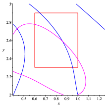
Figure 3: The PM box of a solution of system (6) used in the proof of Theorem 5 (in red). It corresponds to the intersection of the curves defined by the curves $T_{5,1}(x,y)=0$ (in blue) and $T_{5,2}(x,y)=0$ (in magenta).

We take, $g_{1}(y):=T_{5,1}(0.6,y)\cdot T_{5,1}(1,y)$ where

$$T_{5,1}\left(0.6,y\right)={\frac{16679880978201{y}^{11}}{95367431640625}}-{\frac{1167478199895987{y}^{10}}{476837158203125}}+{\frac{6483464101392579{y}^{9}}{476837158203125}}$$

$$-{\frac{86310474195914829{y}^{8}}{2384185791015625}}+{\frac{447004829071396386{y}^{7}}{11920928955078125}}+{\frac{8389294048378453266{y}^{6}}{298023223876953125}}$$

$$-{\frac{148429346693234077422{y}^{5}}{1490116119384765625}}+{\frac{80721993185246247282{y}^{4}}{1490116119384765625}}+{\frac{317995739735111299953{y}^{3}}{7450580596923828125}}$$

$$-{\frac{1653153957629818831467{y}^{2}}{37252902984619140625}}+{\frac{4929661459397407475239y}{931322574615478515625}}+{\frac{3868538667523044137292}{4656612873077392578125}}.$$

​​and

$$T_{5,1}\left(1,y\right)= \left(y-2\right)\times$$

$$\left({y}^{10}-15{y}^{9}+97{y}^{8}-353{y}^{7}+792{y}^{6}-1130{y}^{5}+1022{y}^{4}-566{y}^{3}+177{y}^{2}-27y+1\right).$$

​​and prove that $g_{1}$ it is negative for $y\in[2.3,2.9].$ This can be done by using the Sturm sequences of both polynomials.

Proceeding in an analogous way we obtain that $g_{2}(y):=T_{5,2}(x,2.3)\cdot T_{5,2}(x,2.9)$ is a polynomial of degree $62$ and it is negative for $x\in[0.6,1].$ Hence the map $f=\left(T_{5,1},T_{5,2}\right)$ satisfies the hypothesis of the PMT and there exists a solution of system (6) in $\mathcal{B}$.

(b) By imposing $T^{6}(x,y)=(x,y)$, we get

$$x\cdot T_{6,1}(x,y)=0,\quad y\cdot T_{6,2}(x,y)=0,$$ (8)

where $T_{6,1}$ and $T_{6,2}$ are polynomials with degree 63, and 967 and 910 monomials respectively. We compute the resultants of these polynomials, and remove the repeated factors and those factors corresponding to $x=0$ and $y=0$.

$$P(x):=\frac{\mathrm{Res}(T_{6,1},T_{6,2};y)}{{x}^{420}\left(x^{2}-3x+1\right)\left(x-1\right)^{2}\left(x-2\right)^{405}}=A\,\left({x}^{3}-10{x}^{2}+17x-1\right)\left({x}^{2}-3x+1\right)$$

$$\left({x}^{6}-25{x}^{5}+184{x}^{4}-547{x}^{3}+669{x}^{2}-254x+1\right)\left(128{x}^{12}-2816{x}^{11}+25280{x}^{10}-124256{x}^{9}\right.$$

$$\left.+372768{x}^{8}-713136{x}^{7}+876616{x}^{6}-677024{x}^{5}+309828{x}^{4}-74692{x}^{3}+7552{x}^{2}-272x+1\right)$$

$$\left({x}^{12}-40{x}^{11}+638{x}^{10}-5436{x}^{9}+27664{x}^{8}-88424{x}^{7}+181016{x}^{6}-237152{x}^{5}+195072{x}^{4}\right.$$

$$\left.-96608{x}^{3}+26624{x}^{2}-3456x+128\right)\left({x}^{6}-11{x}^{5}+44{x}^{4}-78{x}^{3}+60{x}^{2}-16x+1\right)\left(x-1\right)$$

$$\left(x-2\right)\left({x}^{3}-9{x}^{2}+14x-1\right),$$

​and

$$Q(y):=\frac{\mathrm{Res}(T_{6,1},T_{6,2};x)}{y^{6}(y-1)(y^{2}-3y+1)}=B\,\left(y-2\right)\left({y}^{3}+26{y}^{2}+104y+104\right)\left({y}^{3}+36{y}^{2}+180y+216\right)$$

$$\left({y}^{6}+182{y}^{5}+3136{y}^{4}+16072{y}^{3}+25872{y}^{2}+15680y+3136\right)\left(128{y}^{12}+23808{y}^{11}+602304{y}^{10}+\right.$$

$$\left.2820832{y}^{9}-4126176{y}^{8}-29841552{y}^{7}+8077160{y}^{6}+52324032{y}^{5}-24120108{y}^{4}-9219772{y}^{3}\right.$$

$$\left.+3690240{y}^{2}-133920y+837\right)\left(16384{y}^{12}+671744{y}^{11}+5943296{y}^{10}+1502208{y}^{9}-62922752{y}^{8}\right.$$

$$\left.-53763840{y}^{7}+165704768{y}^{6}+167848384{y}^{5}-52858224{y}^{4}-48703232{y}^{3}\right.$$

$$\left.+5309928{y}^{2}-133920y+837\right)\left(y-1\right)\left({y}^{2}-3y+1\right),$$

​where $A$ and $B$ are non-zero constants.

By using the Sturm method we obtain that $P(x)$ has 46 different real roots (all of them positive), and $Q(x)$ has 40 different real roots (16 of them positive). Hence, each solution in the positive quadrant of system (8) is contained in isolation in one of the $736=46\times 16$ sets of the form

$$\mathcal{I}_{i,j}=I_{i}\times J_{j},\,i=1,\cdots,46;\,j=1,\ldots,16.$$

where $\{I_{i}\subset\mathbb{R}^{+},$ $i=1,\ldots,46\}$ and $\{J_{j}\subset\mathbb{R}^{+},$ $j=1,\ldots,16\}$ are intervals with rational ends such that each one of them contains a positive root of $P$ and $Q$, respectively, in isolation.

In our computations we have obtained these intervals, with rational ends and maximum length bounded by $10^{-100}$ (in order to apply the discard procedure efficiently). We don’t give these intervals in this paper. But in order to facilitate the reproduction of our results and allow the reader to determine and locate the $6$-periodic orbits, we indicate that these intervals (and therefore the roots) are ordered, in the sense that if $\ell<m$ then $I_{\ell}$ (respectively $J_{\ell}$) is completely to the left of $I_{m}$ (respectively $J_{m}$).

To discard those sets $\mathcal{I}_{i,j}$ that do not contain any solution of system (8), we apply the discard method. The procedure allows to eliminate $717$ boxes. Moreover, the box $\mathcal{I}_{17,12}=[1,1]\times[2,2]$ corresponds with the fixed point $(1,2)$ and the boxes $I_{11,10},$ $I_{17,7},$ $I_{31,7},$ $I_{31,10},$ $I_{17,15}$ and $I_{11,15}$ correspond to the explicit 6-periodic orbit given in the statement. Hence the remaining solutions of system (8) must be contained in one of the following $12$ non-discarded boxes:

$$\mathcal{I}_{8,6},\,\mathcal{I}_{9,3},\,\mathcal{I}_{12,14},\,\mathcal{I}_{13,11},\,\mathcal{I}_{16,16},\,\mathcal{I}_{18,1},\,\mathcal{I}_{20,13},\,\mathcal{I}_{21,8},\,\mathcal{I}_{30,4},\,\mathcal{I}_{34,9},\,\mathcal{I}_{35,2},\,\mathcal{I}_{37,5}.$$ (9)

Again, the PMT can be used to prove that in each of them there is a solution of system (8). Since the solution must be unique, we prove that in total there are $18$ periodic points of minimal period $6$. Since the computation are quite similar to the ones used to study the 5-periodic points we skip them.    

4.1 Determination of the $5$-periodic orbits

By using the boxes computed in the proof of the above result, it is easy to determine which points correspond to each orbit. Indeed, first we concentrate on the $5$-periodic orbits. Let us denote $P_{i,j}=(x,y)$ the (unique) $5$-periodic point lying in the box $\mathcal{I}_{i,j}$ of (7). We notice that the two $5$-periodic orbits of $T$ in $\mathrm{Int}(\triangle)$ are given by $P_{9,10}\rightarrow P_{7,9}\rightarrow P_{8,6}\rightarrow P_{14,3}\rightarrow P_{23,5},$ and $P_{5,7}\rightarrow P_{10,2}\rightarrow P_{20,1}\rightarrow P_{24,4}\rightarrow P_{6,1},$ where

$$\begin{array}[]{|c|}\hline\cr\mbox{Orbit 1}\\ \hline\cr P_{9,10}\simeq\left(0.8581419568,2.587834436\right)\\ \hline\cr P_{7,9}\simeq\left(0.4754309022,2.220729307\right)\\ \hline\cr P_{8,6}\simeq\left(0.6198857282,1.055803338\right)\\ \hline\cr P_{14,3}\simeq\left(1.440807176,0.6544774210\right)\\ \hline\cr P_{23,5}\simeq\left(2.744327621,0.9429757645\right)\\ \hline\cr\end{array}\quad\begin{array}[]{|c|}\hline\cr\mbox{Orbit 2}\\ \hline\cr P_{5,7}\simeq\left(0.3667104103,1.192698099\right)\\ \hline\cr P_{10,2}\simeq\left(0.8949903070,0.4373748091\right)\\ \hline\cr P_{20,1}\simeq\left(2.387507364,0.3914462147\right)\\ \hline\cr P_{24,4}\simeq\left(2.915257323,0.9345807202\right)\\ \hline\cr P_{6,11}\simeq\left(0.4377607446,2.724543288\right)\\ \hline\cr\end{array}$$

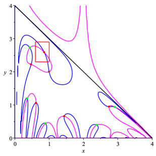
Figure 4: Two $5$-periodic orbits of the map (5) in $\mathrm{Int}(\triangle)$ (Orbit 1 in red and Orbit 2 in green). They correspond to the intersection of the curves defined by the curves $T_{5,1}(x,y)=0$ (in blue) and $T_{5,2}(x,y)=0$ (in magenta). The fixed point $(1,2)$ (in brown). The PM box containing the point $P_{9,10}$ used in the proof of Theorem 5 (in red).

These decimal approximations have obtained using the intervals given in the appendix. Remember that they give an approximation with a maximum error of $10^{-40}.$ The points are depicted in Figure 4.

The above assertions can be proved, by using the fact that taking $\mathcal{I}_{i,j}=[\underline{x},\overline{x}]\times[\underline{y},\overline{y}]$, and setting $(\widetilde{x},\widetilde{y})=T(P_{i,j})$, since $\widetilde{y}=xy$ it must satisfy $\underline{x}\,\underline{y}<\widetilde{y}<\overline{x}\,\overline{y}$, and from these inequalities is easy to identify in which box of (7) is $(\widetilde{x},\widetilde{y})$. For instance, for the point $P_{9,10}\in\mathcal{I}_{9,10}$, and setting $\widetilde{y}=T(P_{9,10})_{2}$, one has that $a:=\underline{x}\,\underline{y}<\widetilde{y}<b:=\overline{x}\,\overline{y}$ where

$$a=\frac{16852116181629561083016478047392649752537328677768476306665633800018763276864769965}{7588550360256754183279148073529370729071901715047420004889892225542594864082845696},$$

$$b=\frac{4213029045407390270754119511848162438134407216162333392848558471828944039611220943}{1897137590064188545819787018382342682267975428761855001222473056385648716020711424}.$$

Now, it is easy to check that the only interval $J_{j}$ for $j\in\{1,2,\ldots,10,11\}$ with nonempty intersection with $(a,b)$ is $J_{9}$, hence $P_{7,9}=T(P_{9,10})$.

4.2 Determination of the $6$-periodic orbits

Proceeding as in the previous section, we determine the points of two of the $6$-periodic orbits. The third one is explicit. Again we denote $P_{i,j}=(x,y)$ the (unique) $6$-periodic point lying in the box $\mathcal{I}_{i,j}$ of (9). The points are depicted in Figure 5.

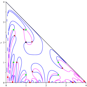
Figure 5: Three $6$-periodic orbits of the map (5) in $\mathrm{Int}(\triangle)$ (Orbit 1,2 and 3 in brown, red and green, respectively). They correspond to the intersection of the curves defined by the curves $T_{6,1}(x,y)=0$ (in blue) and $T_{6,2}(x,y)=0$ (in magenta). The fixed point $(1,2)$ (in black).

We have, Orbit 1: $P_{20,13}\rightarrow P_{16,16}\rightarrow P_{12,14}\rightarrow P_{13,11}\rightarrow P_{21,8}\rightarrow P_{34,9};$ Orbit 2: $P_{8,6}\rightarrow P_{9,3}\rightarrow P_{18,1}\rightarrow P_{35,2}\rightarrow P_{30,4}\rightarrow P_{37,5};$ and Orbit 3: $P_{11,10}\rightarrow P_{17,7}\rightarrow P_{31,7}\rightarrow P_{31,10}\rightarrow P_{17,15}\rightarrow P_{11,15},$ where the points of Orbit 3 are the ones of the statement and

$$\begin{array}[]{|c|}\hline\cr\mbox{Orbit 1}\\ \hline\cr P_{20,13}\simeq\left(1.300802119,2.018868702\right)\\ \hline\cr P_{16,16}\simeq\left(0.8849736378,2.626148686\right)\\ \hline\cr P_{12,14}\simeq\left(0.4326438557,2.324072356\right)\\ \hline\cr P_{13,11}\simeq\left(0.5378990919,1.005495625\right)\\ \hline\cr P_{21,8}\simeq\left(1.321405751,0.5408551836\right)\\ \hline\cr P_{34,9}\simeq\left(2.824820695,0.7146891501\right)\\ \hline\cr\end{array}\quad\begin{array}[]{|c|}\hline\cr\mbox{Orbit 2}\\ \hline\cr P_{8,6}\simeq\left(0.09022635321,0.2685661106\right)\\ \hline\cr P_{9,3}\simeq\left(0.3285328773,0.02423174076\right)\\ \hline\cr P_{18,1}\simeq\left(1.198236734,0.007960923513\right)\\ \hline\cr P_{35,2}\simeq\left(3.347636595,0.009539070990\right)\\ \hline\cr P_{30,4}\simeq\left(2.151942266,0.03193334313\right)\\ \hline\cr P_{37,5}\simeq\left(3.908194837,0.06871871076\right)\\ \hline\cr\end{array}$$

The decimal approximations have obtained using the intervals computed in the proof of Theorem 5. They gave an approximation with a maximum error of $10^{-100}.$ The points are depicted in Figure 5.

5 Limit cycles of piecewise linear differential systems

The study of the number of limit cycles for planar differential systems is a classical topic in the theory of dynamical systems. In the last years, many attention has been devoted to the study of nested limit cycles of piecewise linear systems, steered by the applicability of these systems in the modelling of biological and mechanical applications. In 2012, S.M. Huan and X.S. Yang gave numerical evidences of a piecewise linear system with two zones and a discontinuity straight line, having three nested limit cycles ([18]). A proof based on the Newton–Kantorovich theorem of the existence of these limit cycles for this example and a nearby one, was given by J. Llibre and E. Ponce ([25]). A different proof, from a bifurcation viewpoint, was presented by E. Freire, E. Ponce and F. Torres in [11]. Until now, as far as we know, three is the maximum observed number of limit cycles in piecewise linear differential systems with two zones and a discontinuity straight line, but it is not known if this is the maximum number that such type of systems can have.

In this section we present a new example, again with 3 limit cycles, inspired on the ones given in [18, 25]. The main difference is that our proof of their existence is based on the PMT.

Theorem 6.

The two-zones piecewise linear differential system

$$\dot{\mathbf{x}}=\left\{\begin{array}[]{ll}A^{+}\mathbf{x}&\mbox{if }x\geq 1,\\ A^{-}\mathbf{x}&\mbox{if }x\leq 1,\end{array}\right.$$ (10)

where $\mathbf{x}=(x,y)^{t}$,

$$A^{-}:=\left(\begin{array}[]{cc}\frac{67}{50}&-\frac{833}{125}\\ \frac{1}{2}&-\frac{87}{50}\end{array}\right)\,\mbox{ and }\,A^{+}:=\left(\begin{array}[]{cr}\frac{3}{8}&-1\\ 1&\frac{3}{8}\end{array}\right),$$

has at least three nested hyperbolic limit cycles surrounding the origin.

To prove the above result, we will use systematically the following lemma, that is a straightforward consequence of Taylor’s formula.

Lemma 7.

Set $h(x)=A\cos(\alpha x)+B\sin(\alpha x)+C\mathrm{e}^{\beta x}+D\mathrm{e}^{-\beta x}$, with $A,B,C,D\in{\mathbb{R}}$, $\alpha\neq 0,$ $\beta>0$ and $x\in[\underline{x},\overline{x}]\subset{\mathbb{R}}^{+}$. Then for each $n\geq 0$ we have $h(x)=\sum\limits_{j=0}^{n}a_{j}x^{j}+m_{n}(x)x^{n+1}$, where

$$a_{j}=\frac{1}{j!}\left(\alpha^{j}\left[A\cos\left(j\frac{\pi}{2}\right)+B\sin\left(j\frac{\pi}{2}\right)\right]+\beta^{j}\left[C+(-1)^{j}D\right]\right),$$

$$\left|m_{n}(x)\right|\leq\overline{m}=\frac{\left|\alpha\right|^{n+1}\left(|A|+|B|\right)+\left|\beta\right|^{n+1}\left(|C|\mathrm{e}^{\beta\overline{x}}+|D|\mathrm{e}^{-\beta\underline{x}}\right)}{(n+1)!}.$$ (11)

Proof of Theorem 6.

Let $\varphi^{\pm}(t;p)=(x^{\pm}(t;p),x^{\pm}(t;p))$ denote the flows associated to the linear systems $\dot{\mathbf{x}}=A^{\pm}\mathbf{x}$. Observe that if there exists a limit cycle then it must lie on both sides of the line $x=1$, so let $t^{-}>0$ be the smaller time such that $x^{-}(t^{-};(1,y))=1$ for a point $(1,y)$ with $y>0$, and let $t^{+}>0$ be the smaller time such that $x^{+}(-t^{+};(1,y))=1$. Then any limit cycle must satisfy $x^{+}(-t^{+};(1,y))-1=0,$ $x^{-}(t^{-};(1,y))-1=0,$ $y^{+}(-t^{+};(1,y))-y^{-}(t^{-};(1,y))=0,$ or equivalently

$$\mathrm{e}^{-\frac{3}{8}u}\left(\cos\left(u\right)+y\sin\left(u\right)\right)-1=0,$$ (12)

$$\frac{1}{35}\left(35\cos\left({\frac{49}{50}}v\right)+\left(-238y+55\right)\sin\left({\frac{49}{50}}v\right)\right)\mathrm{e}^{-\frac{1}{5}v}-1=0,$$ (13)

$$\frac{1}{49}\left(-49\cos\left({\frac{49}{50}v}\right)y+\left(77y-25\right)\sin\left({\frac{49}{50}v}\right)\right){{\rm e}^{-\frac{v}{5}}}+{{\rm e}^{-\frac{3}{8}u}}\left(\cos\left(u\right)y-\sin\left(u\right)\right)=0,$$ (14)

where $u=t^{+}>0$ and $v=t^{-}>0$.

By solving equation (12) we get $y=\big{(}\mathrm{e}^{-\frac{3}{8}u}-\cos(u)\big{)}/{\sin(u)}.$ By substituting this expression in equations (13) and (14), we obtain

$$\begin{array}[]{ll}g_{1}(u,v):=&a(v)\cos(u)+b(v)\sin(u)-a(v)\mathrm{e}^{\frac{3}{8}u}=0,\\ g_{2}(u,v):=&c(v)\cos(u)+d(v)\sin(u)+e(v)\mathrm{e}^{\frac{3}{8}u}+f(v)\mathrm{e}^{-\frac{3}{8}u}=0,\end{array}$$ (15)

where

$$\begin{array}[]{ll}a(v)=238\,{{\rm e}^{-\frac{v}{5}}}\sin\left({\frac{49}{50}\,v}\right),&b(v)=55\,{{\rm e}^{-\frac{v}{5}}}\sin\left({\frac{49}{50}\,v}\right)+35\,{{\rm e}^{-\frac{v}{5}}}\cos\left({\frac{49}{50}\,v}\right)-35,\\ \end{array}$$

and

$$\begin{array}[]{ll}c(v)=49\,{{\rm e}^{-\frac{v}{5}}}\cos\left({\frac{49}{50}\,v}\right)-77\,{{\rm e}^{-\frac{v}{5}}}\sin\left({\frac{49}{50}\,v}\right)+49,&d(v)=-25\,{{\rm e}^{-\frac{v}{5}}}\sin\left({\frac{49}{50}\,v}\right),\\ e(v)=77\,{{\rm e}^{-\frac{v}{5}}}\sin\left({\frac{49}{50}\,v}\right)-49\,{{\rm e}^{-\frac{v}{5}}}\cos\left({\frac{49}{50}\,v}\right),&f(v)=-49.\end{array}$$

  

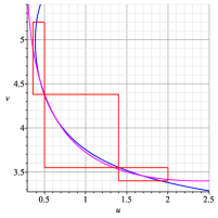
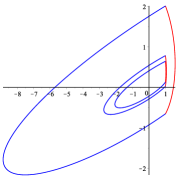
Figure 6: Left part: Intersection points between $g_{1}(u,v)=0$ (in blue) and $g_{2}(u,v)=0$ (in magenta) and some PM boxes containing them. Right part: the 3 limit cycles of system (10).

Numerically it is easy to guess that there are 3 different solutions of system (15), see Figure 6. Their approximate values in $(u,v)$ variables are $(0.441441,4.554696),$ $(0.639391,4.105752)$ and $(1.686596,3.458345).$ Once we prove that near these values there are actual solutions of system (15), each one of them will correspond to a solution of the system of equations (12)–(14) and, consequently, all them will give rise to 3 limit cycles of system (10), see again Figure 6.

To prove the existence of 3 solutions of system (15), we consider the 3 boxes:

$$\mathcal{B}_{1}:=\left[{\frac{9}{25}},\frac{1}{2}\right]\times\left[{\frac{219}{50}},{\frac{26}{5}}\right],\,\mathcal{B}_{2}:=\left[\frac{1}{2},\frac{7}{5}\right]\times\left[\frac{71}{20},{\frac{219}{50}}\right]\,\mathcal{B}_{3}:=\left[\frac{7}{5},2\right]\times\left[{\frac{17}{5}},{\frac{71}{20}}\right]$$

and prove that they are PM boxes for $(g_{1},g_{2}).$

To see that we are under the hypotheses of the PMT, in all the cases we proceed systematically in the following form: We suppose that we want to prove that a function $h(x)$ of the form of Lemma 7 is positive (resp. negative) in $[\underline{x},\overline{x}]\subset{\mathbb{R}}^{+}$. Firstly, we use this lemma to have its Taylor polynomial at $x=0$ up to a certain order $n.$ Secondly, we minorize (resp. majorize) the polynomial by a polynomial with rational coefficients, obtained by truncating the decimal expression up to some suitable order $k$, and subtracting (resp. adding) $10^{-k}$ to the obtained quantity, that is

$$a_{j}^{\pm}:=\mathrm{Trunc}(a_{j}\cdot 10^{k})\cdot 10^{-k}\pm 10^{-k}\in\mathbb{Q},$$

where $\mathrm{Trunc}$ stands for the truncation to the next nearest integer towards $0$. Finally we consider $P_{n,k}^{\pm}(x)=\sum\limits_{j=0}^{n}a_{j}^{\pm}x^{j}\pm Mx^{n+1}$, where $M\in\mathbb{Q}$ is a suitable upper bound of the right-hand side expression in (11), so that

$$P_{n,k}^{-}(x)-Mx^{n+1}\leq h(x)\leq P_{n,k}^{+}(x)+Mx^{n+1}.$$

Now we only have to check if $P_{n,k}^{-}(x)>0$ (resp. $P_{n,k}^{+}(x)<0$) in $[\underline{x},\overline{x}]$. To do this we use the Sturm sequences of these polynomials.

Applying this approach we prove that $\mathcal{B}_{1}$, $\mathcal{B}_{2}$ and $\mathcal{B}_{3}$ are PM boxes by setting the following parameters $n$, $k$ and $M$ in each face (we use the notation $\mathcal{B}=[\underline{u},\overline{u}]\times[\underline{v},\overline{v}]$):

Box $\mathcal{B}_{1}$:

$$\begin{array}[]{|r|c|c|c|c|}\hline\cr\mathrm{Face}&u=\underline{u}&u=\overline{u}&v=\underline{v}&v=\overline{v}\\ \hline\cr\mbox{Target function }h\mbox{ and sign}&g_{1}<0&g_{1}>0&g_{2}>0&g_{2}<0\\ \hline\cr\mbox{Polynomial }&P_{n,k}^{+}&P_{n,k}^{-}&P_{n,k}^{-}&P_{n,k}^{+}\\ \hline\cr\mbox{Parameters: }n&16&16&4&4\\ k&15&15&3&3\\ \hline\cr\mbox{Bound }M&10^{-13}&10^{-12}&\frac{7}{10}&\frac{4}{5}\\ \hline\cr\end{array}$$

Box $\mathcal{B}_{2}$:

$$\begin{array}[]{|r|c|c|c|c|}\hline\cr\mathrm{Face}&u=\underline{u}&u=\overline{u}&v=\underline{v}&v=\overline{v}\\ \hline\cr\mbox{Target function }h\mbox{ and sign}&\mathrm{e}^{\frac{v}{5}}\cdot g_{2}>0&\mathrm{e}^{\frac{v}{5}}\cdot g_{2}<0&g_{1}<0&g_{1}>0\\ \hline\cr\mbox{Polynomial }&P_{n,k}^{-}&P_{n,k}^{+}&P_{n,k}^{+}&P_{n,k}^{-}\\ \hline\cr\mbox{Parameters: }n&16&16&6&4\\ k&14&10&2&2\\ \hline\cr\mbox{Bound }M&10^{-13}&10^{-12}&\frac{1}{50}&\frac{13}{10}\\ \hline\cr\end{array}$$

Box $\mathcal{B}_{3}$:

$$\begin{array}[]{|r|c|c|c|c|}\hline\cr\mathrm{Face}&u=\underline{u}&u=\overline{u}&v=\underline{v}&v=\overline{v}\\ \hline\cr\mbox{Target function }h\mbox{ and sign}&\mathrm{e}^{\frac{v}{5}}\cdot g_{1}<0&\mathrm{e}^{\frac{v}{5}}\cdot g_{1}>0&g_{2}>0&g_{2}<0\\ \hline\cr\mbox{Polynomial }&P_{n,k}^{+}&P_{n,k}^{-}&P_{n,k}^{-}&P_{n,k}^{+}\\ \hline\cr\mbox{Parameters: }n&13&11&6&7\\ k&8&8&3&2\\ \hline\cr\mbox{Bound }M&10^{-8}&10^{-6}&10^{-2}&10^{-2}\\ \hline\cr\end{array}$$

We only give details of some of the computations for $\mathcal{B}_{1}$. For instance we show that $g_{2}(u,\underline{v})>0$ for all $u\in[\underline{u},\overline{u}]$. All the other computations can be reproduced using the information given above. Indeed, we take $\mathcal{B}_{1}$ and we observe that

$$g_{2}(u,\underline{v})=c\left({\frac{219}{50}}\right)\cos(u)+d\left(\frac{219}{50}\right)\sin(u)+e\left({\frac{219}{50}}\right)\mathrm{e}^{\frac{3}{8}u}+f\left({\frac{219}{50}}\right)\mathrm{e}^{-\frac{3}{8}u},$$

which has the form of the function $h$ in Lemma 7, where

$$\begin{array}[]{l}A=c\left(\frac{219}{50}\right)=49\,{{\rm e}^{-{\frac{219}{250}}}}\cos\left({\frac{10731}{2500}}\right)-77\,{{\rm e}^{-{\frac{219}{250}}}}\sin\left({\frac{10731}{2500}}\right)+49,\\ B=d\left(\frac{219}{50}\right)=-25\,{{\rm e}^{-{\frac{219}{250}}}}\sin\left({\frac{10731}{2500}}\right),\\ C=e\left(\frac{219}{50}\right)=\left(-49\,\cos\left({\frac{10731}{2500}}\right)+77\,\sin\left({\frac{10731}{2500}}\right)\right){{\rm e}^{-{\frac{219}{250}}}},\\ D=f\left(\frac{219}{50}\right)=-49.\end{array}$$

By applying this lemma with $n=4,$ we obtain $P_{4}(u)=\sum_{j=0}^{4}a_{j}u^{j}.$ After taking $a_{j}^{-}:=\mathrm{Trunc}(a_{j}\cdot 10^{3})\cdot 10^{-3}-10^{-3}$ for each $j=0,\ldots,4$ we get

$$P_{4,3}^{-}(u)=-{\frac{1}{1000}}+{\frac{1001}{50}\,u}-{\frac{39899}{1000}\,{u}^{2}}-{\frac{669}{500}\,{u}^{3}}+{\frac{357}{125}\,{u}^{4}}.$$

By using (11) we also obtain that

$$\overline{m}_{4}=\left({\frac{49\,{{\rm e}^{-{\frac{219}{250}}}}}{120}}+{\frac{3969\,{{\rm e}^{-{\frac{1377}{2000}}}}}{1310720}}\right)\cos\left({\frac{10731}{2500}}\right)+\\ \left(-{\frac{17\,{{\rm e}^{-{\frac{219}{250}}}}}{20}}-{\frac{6237\,{{\rm e}^{-{\frac{1377}{2000}}}}}{1310720}}\right)\sin\left({\frac{10731}{2500}}\right)+{\frac{49}{120}}+{\frac{3969\,{{\rm e}^{-{\frac{27}{200}}}}}{1310720}}\simeq 0.6664<\frac{7}{10}=M.$$

By using the Sturm sequence of $P_{4,3}^{-}(u)-Mu^{5}$ we prove that it has no roots in $[\underline{u},\overline{u}]$ and, moreover, it is positive in this interval. Hence $0<P_{4,3}^{-}(u)-Mu^{5}<g_{2}(u,\underline{v})\,\mbox{ for all }u\in[\underline{u},\overline{u}].$

To prove the hyperbolicity of the limit cycles we can follow the same ideas that in [25].     

6 On the existence of a symmetric central configuration

Central configurations are a very special type of solutions of the $N$-body problem in Celestial Mechanics, in which the acceleration of every body is proportional to the position vector of the body with respect the center of mass of the system. They play an important role in practical applications and there is a vast literature on the topic, both classical and recent. An account of known facts and open problems can be found in [24].

In the $(1+n)$-body problem it is supposed that there is one body with a large mass and $n$ bodies whose masses can be neglected in comparison with the large one. These bodies are named as infinitesimal masses. With our approach we prove in a very simple way the existence of a special planar central configurations of the $(1+4)$-body problem, already given in [8].

According to the results in [4, 8], all planar central configurations in the $(1+n)$-body problem lie on a circle centered at the position of the large mass. Furthermore, denoting by $\alpha_{i}\in\mathbb{S}^{1},$ with $\alpha_{1}<\alpha_{2}<\ldots<\alpha_{n},$ the angles defined by the position of the $i$th infinitesimal masses on a circle centered at the origin, central configurations must satisfy the system of $n$ equations, $i=1,\ldots,n,$

$$\sum\limits_{j=1}^{n}f(\alpha_{j}-\alpha_{i})=0,\quad\mbox{with}\quad f(\theta):=\Big{(}1-\dfrac{\sqrt{2}}{4\sqrt{(1-\cos(\theta))^{3}}}\Big{)}\sin(\theta).$$

Notice that $f(-\theta)=-f(\theta).$

When $n=4,$ we introduce the variables $u=\alpha_{2}-\alpha_{1},$ $v=\alpha_{3}-\alpha_{1}$ and $w=\alpha_{4}-\alpha_{1}.$ Then the above system is equivalent to the system (with only 3 equations):

$$f(u)+f(v)+f(w)=0,-f(u)+f(v-u)+f(w-u)=0,-f(v)+f(u-v)+f(w-v)=0.$$

Although our point of view could be applied to prove the existence of solutions of the above system (and so of central configurations), for simplicity we will look for a symmetric one, the one satisfying tat $\alpha_{4}-\alpha_{3}=\alpha_{2}-\alpha_{1}$. In our coordinates this implies that $w=u+v$ and hence the system reduces to the system with 2 equations

$$g_{1}(u,v):=f(u)+f(v)+f(u+v)=0,\quad g_{2}(u,v):=f(u)-f(v)-f(v-u)=0.$$

​​​

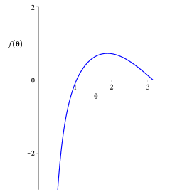
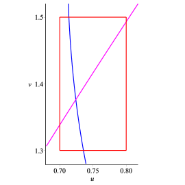
Figure 7: Left figure: graph of $f(\theta)$ in $(0,\pi]$. Right figure: intersection of the curves $g_{1}(u,v)=0$ (in blue) and $g_{2}(u,v)=0$ (in magenta). In red, a PM box.

Let us prove that we can apply PMT to the box $[0.7,0.8]\times[1.3,1.5],$ see Figure 7. To simplify the notation we denote by $g_{i}(I)+g_{j}(J)$ the set of all values $g_{i}(x)+g_{j}(y),$ with $x\in I$ and $y\in J.$ Then, simply using that $f$ is increasing between in $(0,\theta^{*})$ and decreasing in $(\theta^{*},\pi)$, where $\theta^{*}\simeq 1.891\in(1.8,1.9)$, see again Figure 7, we get:

$$\left.g_{1}(0.7,v)\right|_{v\in[1.3,1.5]} =\left.f(0.7)+f(v)+f(0.7+v)\right|_{v\in[1.3,1.5]}$$

$$=f(0.7)+f([1.3,1.5])+f([2,2.2])$$

$$\leq f(0.7)+f(1.5)+f(2)\simeq-0.031<0.$$

Similarly, $\left.g_{1}(0.8,v)\right|_{v\in[1.3,1.5]}=f(0.8)+f([1.3,1.5])+f([2.1,2.3])\geq f(0.8)+f(1.3)+f(2.3)\simeq 0.24>0,$ $\left.g_{2}(u,1.3)\right|_{u\in[0.7,0.8]}=f([0.7,0.8])-f(1.3)-f([0.5,0.6])\geq f(0.7)-f(1.3)-f(0.6)\simeq 0.40>0,$ and $\left.g_{2}(u,1.5)\right|_{u\in[0.7,0.8]}=f([0.7,0.8])-f(1.5)-f([0.7,0.8])\leq f(0.8)-f(1.5)-f(0.7)\simeq-0.052<0.$ Hence we have proved the existence of a symmetric central configuration for this problem. In fact, numerically this solution is $u=u^{*}\simeq 0.7242718590,$ $v=v^{*}\simeq 1.376255451$ and it corresponds with the values $x^{*}=\cos((u^{*}+v^{*})/4)\simeq 0.86525786$ and $y^{*}=\sin((v^{*}-u^{*})/4)\simeq 0.162275119$ given in the proof of [8, Prop 13] and found using the variables $x=\cos((\alpha_{2}+\alpha_{3}-2\alpha_{1})/4)$ and $y=\sin((\alpha_{3}-\alpha_{2})/4).$

Appendix.

The 32 intervals of maximum length $10^{-40}$ containing in isolation the positive roots of the polynomial $P(x)$ that appear in the proof of Theorem 1 are:

$$I_{1}=\left[{\frac{30416172743817963645774671148052190959399}{178405961588244985132285746181186892047843328}},{\frac{60832345487635927291549342296104381918799}{356811923176489970264571492362373784095686656}}\right],$$

$$I_{2}=,\left[{\frac{61004111234951360792324423318169046946281}{356811923176489970264571492362373784095686656}},{\frac{30502055617475680396162211659084523473141}{178405961588244985132285746181186892047843328}}\right],$$

$$I_{3}=,\left[{\frac{27421400457977260353638941607050001933877}{11150372599265311570767859136324180752990208}},{\frac{54842800915954520707277883214100003867755}{22300745198530623141535718272648361505980416}}\right],$$

$$I_{4}=,\left[{\frac{55177596464914226273769532370430091204151}{22300745198530623141535718272648361505980416}},{\frac{6897199558114278284221191546303761400519}{2787593149816327892691964784081045188247552}}\right],$$

$$I_{5}=,\left[{\frac{63889964233534261969205802666073326201313}{174224571863520493293247799005065324265472}},{\frac{31944982116767130984602901333036663100657}{87112285931760246646623899502532662132736}}\right],$$

$$I_{6}=,\left[{\frac{76268678313703396955788049048149760899577}{174224571863520493293247799005065324265472}},{\frac{38134339156851698477894024524074880449789}{87112285931760246646623899502532662132736}}\right],$$

$$I_{7}=,\left[{\frac{82831745394319077306596661336176030777141}{174224571863520493293247799005065324265472}},{\frac{41415872697159538653298330668088015388571}{87112285931760246646623899502532662132736}}\right],$$

$$I_{8}=,\left[{\frac{26999831398533091510037286533787056284381}{43556142965880123323311949751266331066368}},{\frac{53999662797066183020074573067574112568763}{87112285931760246646623899502532662132736}}\right],$$

$$I_{9}=,\left[{\frac{74754707508083115080188235040108949111941}{87112285931760246646623899502532662132736}},{\frac{37377353754041557540094117520054474555971}{43556142965880123323311949751266331066368}}\right],$$

$$I_{10}=,\left[{\frac{77964651533856060199939131867310019005089}{87112285931760246646623899502532662132736}},{\frac{38982325766928030099969565933655009502545}{43556142965880123323311949751266331066368}}\right],$$

$$I_{11}=,\left[1,1\right],$$

$$I_{12}=,\left[{\frac{238239449906197613139925190460054741169}{170141183460469231731687303715884105728}},{\frac{121978598351973177927641697515548027478529}{87112285931760246646623899502532662132736}}\right],$$

$$I_{13}=,\left[{\frac{61150748376490059476117465769766977687027}{43556142965880123323311949751266331066368}},{\frac{122301496752980118952234931539533955374055}{87112285931760246646623899502532662132736}}\right],$$

$$I_{14}=,\left[{\frac{31378001665582463990512894476418249863733}{21778071482940061661655974875633165533184}},{\frac{125512006662329855962051577905672999454933}{87112285931760246646623899502532662132736}}\right],$$

$$I_{15}=,\left[{\frac{173371830902734537060512513441447388046677}{87112285931760246646623899502532662132736}},{\frac{86685915451367268530256256720723694023339}{43556142965880123323311949751266331066368}}\right],$$

$$I_{16}=,\left[{\frac{43530335013270399357309383085115875521389}{21778071482940061661655974875633165533184}},{\frac{174121340053081597429237532340463502085557}{87112285931760246646623899502532662132736}}\right],$$

$$I_{17}=,\left[2,2\right],$$

$$I_{18}=,\left[{\frac{43581896065820670510185474007765782536433}{21778071482940061661655974875633165533184}},{\frac{174327584263282682040741896031063130145733}{87112285931760246646623899502532662132736}}\right],$$

$$I_{19}=,\left[{\frac{175074047096038860833682791052723868617523}{87112285931760246646623899502532662132736}},{\frac{43768511774009715208420697763180967154381}{21778071482940061661655974875633165533184}}\right],$$

$$I_{20}=,\left[{\frac{207981224135133170727752198124246427433217}{87112285931760246646623899502532662132736}},{\frac{103990612067566585363876099062123213716609}{43556142965880123323311949751266331066368}}\right],$$

$$I_{21}=,\left[{\frac{53389351149121164414177573637629460658781}{21778071482940061661655974875633165533184}},{\frac{213557404596484657656710294550517842635125}{87112285931760246646623899502532662132736}}\right],$$

$$I_{22}=,\left[{\frac{213578718968144293553725465775995745176425}{87112285931760246646623899502532662132736}},{\frac{106789359484072146776862732887997872588213}{43556142965880123323311949751266331066368}}\right],$$

$$I_{23}=,\left[{\frac{59766163097780263153587646066230635923515}{21778071482940061661655974875633165533184}},{\frac{239064652391121052614350584264922543694061}{87112285931760246646623899502532662132736}}\right],$$

$$I_{24}=,\left[{\frac{253954729472389360941133632461626408129629}{87112285931760246646623899502532662132736}},{\frac{126977364736194680470566816230813204064815}{43556142965880123323311949751266331066368}}\right],$$

$$I_{25}=,\left[{\frac{243357617176921003857605925220978518350987}{43556142965880123323311949751266331066368}},{\frac{486715234353842007715211850441957036701975}{87112285931760246646623899502532662132736}}\right],$$

$$I_{26}=,\left[{\frac{487996318307203475975406100394067486420489}{87112285931760246646623899502532662132736}},{\frac{243998159153601737987703050197033743210245}{43556142965880123323311949751266331066368}}\right],$$

$$I_{27}=,\left[{\frac{854083577046230668182843971813839810572423}{87112285931760246646623899502532662132736}},{\frac{106760447130778833522855496476729976321553}{10889035741470030830827987437816582766592}}\right],$$

$$I_{28}=,\left[{\frac{854169231180689628527098761743375311769429}{87112285931760246646623899502532662132736}},{\frac{427084615590344814263549380871687655884715}{43556142965880123323311949751266331066368}}\right],$$

$$I_{29}=,\left[{\frac{562325002245556480093549131285848700772183}{21778071482940061661655974875633165533184}},{\frac{2249300008982225920374196525143394803088733}{87112285931760246646623899502532662132736}}\right],$$

$$I_{30}=,\left[{\frac{2252874711653478373358567435415938516285773}{87112285931760246646623899502532662132736}},{\frac{1126437355826739186679283717707969258142887}{43556142965880123323311949751266331066368}}\right],$$

$$I_{31}=,\left[{\frac{10605493671441752150124990095059709232394013}{87112285931760246646623899502532662132736}},{\frac{5302746835720876075062495047529854616197007}{43556142965880123323311949751266331066368}}\right],$$

$$I_{32}=,\left[{\frac{10620731390948027186722372703422173139084449}{87112285931760246646623899502532662132736}},{\frac{5310365695474013593361186351711086569542225}{43556142965880123323311949751266331066368}}\right].$$

The 11 intervals of maximum length $10^{-40}$ containing in isolation the positive roots of the polynomial $Q(y)$ are:

$$J_{1}=\left[{\frac{34099774584992488192779339819330125093373}{87112285931760246646623899502532662132736}},{\frac{68199549169984976385558679638660250186747}{174224571863520493293247799005065324265472}}\right],$$

$$J_{2}=\left[{\frac{76201438867882234589322968824595491762585}{174224571863520493293247799005065324265472}},{\frac{38100719433941117294661484412297745881293}{87112285931760246646623899502532662132736}}\right],$$

$$J_{3}=\left[{\frac{7126628029028087048991427050514157728201}{10889035741470030830827987437816582766592}},{\frac{57013024232224696391931416404113261825609}{87112285931760246646623899502532662132736}}\right],$$

$$J_{4}=\left[{\frac{20353365730967257062570091063747267693705}{21778071482940061661655974875633165533184}},{\frac{81413462923869028250280364254989070774821}{87112285931760246646623899502532662132736}}\right],$$

$$J_{5}=\left[{\frac{20536193605572751128435745571834887603857}{21778071482940061661655974875633165533184}},{\frac{82144774422291004513742982287339550415429}{87112285931760246646623899502532662132736}}\right],$$

$$J_{6}=\left[{\frac{5748340141743633609606285424423240727937}{5444517870735015415413993718908291383296}},{\frac{91973442267898137753700566790771851646993}{87112285931760246646623899502532662132736}}\right],$$

$$J_{7}=\left[{\frac{103898657804950550140822640990534612319235}{87112285931760246646623899502532662132736}},{\frac{25974664451237637535205660247633653079809}{21778071482940061661655974875633165533184}}\right],$$

$$J_{8}=\left[2,2\right],$$

$$J_{9}=\left[{\frac{193452806356507885400952564030524665947305}{87112285931760246646623899502532662132736}},{\frac{96726403178253942700476282015262332973653}{43556142965880123323311949751266331066368}}\right],$$

$$J_{10}=\left[{\frac{225432173349181613519899061972772631001865}{87112285931760246646623899502532662132736}},{\frac{112716086674590806759949530986386315500933}{43556142965880123323311949751266331066368}}\right],$$

$$J_{11}=\left[{\frac{237341193967033134227594463359390906202991}{87112285931760246646623899502532662132736}},{\frac{14833824622939570889224653959961931637687}{5444517870735015415413993718908291383296}}\right].$$

References

- [1] Y. Avishai, D. Berend. Transmission through a Thue-Morse chain, Phys. Rev. B. 45 (1992), 2717–2724.
- [2] F. Balibrea, J.L. García Guirao, M. Lampart, J. Llibre. Dynamics of a Lotka-Volterra map, Fundamenta Mathematicae 191 (2006), 265–279.
- [3] J. Bernat, J. Llibre. Counterexample to Kalman and Markus-Yamabe conjectures in dimension larger than 3, Dynam. Contin. Discrete Impuls. Systems 2 (1996), 337–379.
- [4] J. Casasayas, J. Llibre, A. Nunes. Central configurations of the planar -body problem. Celestial Mech. Dynam. Astronom. 60 (1994), 273–288.
- [5] A. Cima, A. Gasull, F. Mañosas. The discrete Markus-Yamabe problem, Nonlinear Anal. TMA 35 (1999), 343–354.
- [6] A. Cima, A. Gasull, F. Mañosas. On the global asymptotic stability of difference equations satisfying a Markus-Yamabe condition, Publ. Mat. Extra vol. (2014), 167–178.
- [7] A. Cima, A. van den Essen, A. Gasull, E. Hubbers, F. Mañosas. A polynomial counterexample to the Markus-Yamabe conjecture, Adv. Math. 131 (1997), 453–457.
- [8] J. M. Cors, J. Llibre, M. Ollé. Central configurations of the planar coorbital satellite problem, Celestial Mech. Dynam. Astronom. 89 (2004), 319–342.
- [9] A. Dickenstein, J. M. Rojas, K. Rusek, J. Shih. Extremal Real Algebraic Geometry and -Discriminants. Moscow Math. Journal 7 (2007), 425–452.
- [10] G.H. Erjaee, F.M. Dannan. Stability analysis of periodic solutions to the nonstandard discretized model of the Lotka-Volterra predator-prey system, Int. J. Bifurcation and Chaos 14 (2004), 4301–4308.
- [11] E. Freire, E. Ponce, F. Torres. The discontinuous matching of two planar linear foci can have three nested crossing limit cycles, Publ. Mat. Extra vol. (2014), 221–253.
- [12] J. García-Saldaña, A. Gasull, H. Giacomini. Bifurcation diagram and stability for a one–parameter family of planar vector fields, J. Math. Anal. Appl. 413 (2014), 321–342.
- [13] J. García-Saldaña, A. Gasull, H. Giacomini. Bifurcation values for a familiy of planar vector fields of degree five. Discrete Contin. Dyn. Syst., 35 (2015), 669–701.
- [14] A. Gasull, M. Llorens, V. Mañosa. Periodic points of a Landen transformation, Commun. Nonlinear Sci. Numer. Simulat. 64 (2018) 232–245.
- [15] A. Granas, J. Dugundji. Fixed point theory. Springer, New York 2003.
- [16] C. Gutierrez. A solution to the bidimensional global asymptotic stability conjecture, Ann. Inst. H. Poincaré Anal. Non Linéaire 12 (1995), 627–671.
- [17] B. Haas. A simple counterexample to Kouchnirenko’s conjecture, Beiträge zur Algebra und Geometrie 43 (2002), 1–8.
- [18] S.M. Huan, X.S. Yang. On the number of limit cycles in general planar piecewise linear systems, Discrete Contin. Dyn. Syst. 32 (2012), 2147–2164.
- [19] E. Isaacson, H.B. Keller. Analysis of numerical methods. Dover Publications, New York 1994.
- [20] A.G. Khovanskiĭ On a class of systems of transcendental equations Doklady Akad. Nauk. SSSR, 255 (1980), 804–807; Soviet Math. Dokl. 22 (1980) 762–765.
- [21] W. Kulpa. The Poincaré-Miranda Theorem, Amer. Math. Month. 104 (1997), 545–550.
- [22] J.P. La Salle. The stability of Dynamical Systems, CBMS-NSF Regional Conference Series in Applied Math. 25, SIAM 1976, (2nd printing 1993).
- [23] T.-Y. Li, J.M. Rojas, X. Wang. Counting real connected components of trinomial curve intersections and -nomial hypersurfaces, Discrete Comput. Geom. 30 (2003), 379–414.
- [24] J. Llibre. On the central configurations of the -body problem, Preprint. November, 2017.
- [25] J. Llibre, E. Ponce. Three nested limit cycles in discontinuous piecewise linear differential systems with two zones, Dynam. Contin. Discrete Impuls. Systems 19 (2012), 325–335.
- [26] P. Malic̆ký. Interior periodic points of a Lotka-Volterra map, J. Difference Eq. Appl. 18 (2012), 553–567.
- [27] L. Markus, H. Yamabe. Global stability criteria for differential systems, Osaka Math. Journal 12 (1960), 305–317.
- [28] C. Miranda. Un’osservazione su un teorema di Brouwer, Boll. Unione Mat. Ital. 3 (1940), 527–527.
- [29] H. Poincaré. Sur certaines solutions particulieres du probléme des trois corps, C. R. Acad. Sci. Paris 97 (1883), 251–252; and Bull. Astronomique 1 (1884), 63–74.
- [30] H. Poincaré. Sur les courbes définies par une équation différentielle IV, J. Math. Pures Appl. 85 (1886), 151–217.
- [31] A.N. Sharkovskiĭ. Low dimensional dynamics, Tagungsbericht 20/1993, Proceedings of Mathematisches Forschungsinstitut Oberwolfach, 1993, 17.
- [32] J. Stoer, R. Bulirsch. Introduction to Numerical Analysis. Springer, New York 2002.
- [33] M.N. Vrahatis. A short proof and a Generalization of Miranda’s existence Theorem, Proc. AMS 107 (1989), 701–703.