A Conjugate-Gradient Approach to the Parameter Estimation Problem of Magnetic Resonance Advection Imaging

Abstract

We consider the inverse problem of estimating the spatially varying pulse wave velocity in blood vessels in the brain from dynamic MRI data, as it appears in the recently proposed imaging technique of Magnetic Resonance Advection Imaging (MRAI). The problem is formulated as a linear operator equation with a noisy operator and solved using a conjugate gradient type approach. Numerical examples on experimental data show the usefulness and advantages of the developed algorithm in comparison to previously proposed methods.

Keywords. Brain Imaging, MRI, Cerebral Hemodynamics, Pulse Wave Velocity, Magnetic Resonance Advection Imaging, Inverse Problems, Space-Time Discretization, Regularization, CGNE

1 Introduction

With every beat of the human heart a pulse wave is created which travels through the blood vessels in the body somewhat like the waves produced by a rock thrown into the water. The speed of the this wave, termed pulse wave velocity (PWV), is closely related to material properties of the blood vessel it travels through [14, 20, 11]; a high PWV indicates a stiffer blood vessel than a lower PWV, given the same vessel wall thickness and vessel diameter. Arterial pulse wave velocity (PWV) is the gold standard for aortic stiffness assessment in cardiovascular disease [13, 16, 28] and provides normative values for healthy and increased arterial stiffness [18, 2, 17]. Arterial stiffness is related to arterial compliance [4, 3, 27], the ratio of blood volume change to blood pressure change. Arterial compliance absorbs the impact of the pulse pressure waves and enables steady blood flow throughout the whole cardiac cycle [6, 26]. Pulse wave velocity and arterial compliance are reliable prognostic markers for cardiovascular morbidity and mortality in adult populations such as the elderly, subjects with diabetes, arteriosclerosis, coronary heart disease, and hypertension [12, 15, 1, 8, 21, 9, 23, 19, 18, 2, 17].

It would be desirable if measurements of the PWV could not only be performed for the major arteries in the body but also in the brain using Magnetic Resonance Imaging (MRI). Brain MRI already provides high-resolution angiograms of arteries deep inside the brain. Adding the pulsatile component of blood flow could allow for the measurement of the cerebral PWV along cerebral arteries. The long-term goal would be to provide a novel clinical biomarker to assess cerebrovascular integrity, namely the cerebrovascular PWV. As a first attempt to non-invasively measure the PWV using MRI, Voss et al. [25]recently introduced the technique of Magnetic Resonance Advection Imaging (MRAI). They propose to measure the pulsatile component of blood flow from dynamic echo-planar imaging (EPI) data, such as acquired in functional and resting-state functional MRI experiments [24, 22]. The fundamental idea is that the PWV and the associated MRI data can be connected via the advection equation

$$\frac{\partial}{\partial t}\rho(x,y,z,t)+v(x,y,z)\cdot\nabla\rho(x,y,z,t)=0\,,$$ (1.1)

where $\rho(x,y,z,t)$ denotes the time-dependent MRI data and $v(x,y,z)$ the spatially varying PWV, which is assumed to be divergence-free. Equation (1.1) was derived from physical considerations and multiple regression was used to estimate $v(x,y,z)$. While leading to promising first results, for example a correct identification of the pulse wave direction following the main cerebral arteries, it was determined that this approach is not suitable to quantitatively estimate the PWV. The main reason is insufficient accuracy of the EPI data and limited temporal resolution.

Hence, in [10] the authors proposed a stable and efficient algorithm for estimating $v(x,y,z)$ via (1.1) based on a formulation of this parameter estimation problem within the framework of Inverse Problems [5]. The resulting nonlinear inverse problem was solved using a fast gradient-based iterative regularization method, which yielded stable reconstructions of the PWV in a reasonable computational time for the given spatio-temporal resolution of the considered MRI data sets. Unfortunately, as with the regression approach, only qualitative estimates of the PWV could be obtained, since the spatio-temporal resolution of the MRI data set was too low to yield quantitative results. However, it is expected that the resolution of MRI data will increase in the years to come, hopefully allowing also quantitative estimates of the PWV. While the algorithm proposed in [10] is, in principle, able to deal with data sets of higher resolution, it may, in practice, not be able to handle the resulting large amount of data in a reasonable time. Thus, there is the need for a faster and robust algorithm for estimating the PWV, which scales well with respect to the size of the involved data sets.

In this paper, we present an algorithm satisfying the above requirements, which is based on a reformulation of the problem into a linear system of equations with both a noisy operator and a noisy right-hand side. This system is then solved by the method of Conjugate Gradients for the Normal Equations (CGNE), where the required calculations can be written down explicitly in terms of simple calculations without having to assemble or store the system matrix, which allows for effective implementation. The remaining part of this paper is structured as follows: in Section 2, we derive the exact mathematical model and reformulate the problem into a system of linear equations, based on a suitable space-time discretization of the problem. In Section 3, we consider the application of CGNE to the problem, deriving an explicit algorithm to carry out the required computations, and which avoids the assembly of the system matrix. In Section 4, we present numerical results of the application of our algorithm to experimental data, and finally, in Section 5, we give some short conclusions.

Since the aim of this paper is mainly the design and presentation of an effective algorithm for solving the parameter estimation problem of MRAI, the interested reader is referred to [25, 10]for a detailed medical and physical background on MRAI.

2 Mathematical Model and Discretization

In this section, we consider a suitable mathematical model and numerical discretization for the parameter estimation problem of MRAI, leading to a linear inverse problem with both a noisy operator and a noisy right-hand side.

As originally proposed in [25], the physics-based model of MRAI implied that the MRI signal $\rho$ is a conserved quantity advected (transported) by the velocity vector field $v$. In its general form, the advection (transport, continuity) equation is given by

$$\rho_{t}(x,y,z,t)+\nabla\cdot(\rho(x,y,z,t)\,v(x,y,z))=0\,,\qquad(x,y,z)\in\Omega\,,t\in[0,T]\,.$$ (2.1)

Under the assumption of a divergence-free vector field $v$, which is reasonable for an incompressible flow, this leads to model equation (1.1) used in [25, 10]. However, since this assumption does not necessarily hold in practice, we directly work with equation (2.1) here.

A typical MRI data set does not provide continuous information over the whole area of the brain but rather consists of averaged values given on a voxel grid. Hence, we assume (for simplicity) that the domain $\Omega$ corresponding to the observed region of the brain is a cuboid. Furthermore, since the voxels are typically uniform, we set

$$x_{i}:=x_{0}+i\Delta x\,,\quad y_{j}:=y_{0}+j\Delta y\,,\quad z_{k}:=z_{0}+k\Delta z\,,$$

and define the voxels $\Omega_{i,j,k}:=[x_{i-1},x_{i}]\times[y_{j-1},y_{j}]\times[z_{k-1},z_{k}]$. Then it follows from integrating (2.1) over the sets $\Omega_{i,j,k}$ that

$$\frac{\partial}{\partial t}\int_{\Omega_{i,j,k}}\rho(x,y,z,t)\,d(x,y,z)+\int_{\partial\Omega_{i,j,k}}\rho(x,y,z,t)\,v(x,y,z)\cdot n(x,y,z)\,dS=0\,,$$ (2.2)

where $n(x,y,z)$ denotes the unit outward normal and $1\leq i\leq I$, $1\leq j\leq J$, $1\leq k\leq K$.

Since neither $\rho$ nor $v$ are known everywhere, all integrals are approximated using some quadrature rules. If one uses midpoint rules, then the values at the boundaries of $\Omega_{i,j,k}$ have to be approximated via interpolation. Therefore, we suggest the following rules that are exact for bilinear and trilinear functions, respectively:

$$\int_{x_{i-1}}^{x_{i}}\int_{y_{j-1}}^{y_{j}}f(x,y)\,d(x,y)\approx{} \frac{\Delta x\Delta y}{4}\Big{(}f(x_{i-1},y_{j-1})+f(x_{i},y_{j-1})$$

$$\hskip 42.67912pt+\,f(x_{i-1},y_{j})+f(x_{i},y_{j})\Big{)},$$

$$\int_{x_{i-1}}^{x_{i}}\int_{y_{j-1}}^{y_{j}}\int_{z_{k-1}}^{z_{k}}f(x,y,z)\,d(x,y,z)\approx{} \frac{\Delta x\Delta y\Delta z}{8}\Big{(}f(x_{i-1},y_{j-1},z_{k-1})+f(x_{i},y_{j-1},z_{k-1})$$

$$\hskip 56.9055pt+\,f(x_{i-1},y_{j},z_{k-1})+f(x_{i},y_{j},z_{k-1})$$

$$\hskip 56.9055pt+\,f(x_{i-1},y_{j-1},z_{k})+f(x_{i},y_{j-1},z_{k})$$

$$\hskip 56.9055pt+\,f(x_{i-1},y_{j},z_{k})+f(x_{i},y_{j},z_{k})\Big{)}.$$

Thus, we obtain the semi-discrete system

$$\frac{\partial}{\partial t}D_{i,j,k}(t)=\frac{2}{\Delta x}A_{i,j,k}(t)+\frac{2}{\Delta y}B_{i,j,k}(t)+\frac{2}{\Delta z}C_{i,j,k}(t)\,,$$ (2.3)

where $1\leq i\leq I$, $1\leq j\leq J$, $1\leq k\leq K$,

$$D_{i,j,k}(t):={} \rho_{i-1,j-1,k-1}(t)+\rho_{i,j-1,k-1}(t)+\rho_{i-1,j,k-1}(t)+\rho_{i,j,k-1}(t)$$

$$+\,\rho_{i-1,j-1,k}(t)+\rho_{i,j-1,k}(t)+\rho_{i-1,j,k}(t)+\rho_{i,j,k}(t)\,,$$

$$A_{i,j,k}(t):={} \Big{(}\rho_{i-1,j-1,k-1}(t)\,v_{1,i-1,j-1,k-1}+\rho_{i-1,j,k-1}(t)\,v_{1,i-1,j,k-1}$$

$$\;\;+\,\rho_{i-1,j-1,k}(t)\,v_{1,i-1,j-1,k}+\rho_{i-1,j,k}(t)\,v_{1,i-1,j,k}\Big{)}$$

$$-\,\Big{(}\rho_{i,j-1,k-1}(t)v_{1,i,j-1,k-1}+\rho_{i,j,k-1}(t)v_{1,i,j,k-1}$$

$$\quad\;\,+\,\rho_{i,j-1,k}(t)v_{1,i,j-1,k}+\rho_{i,j,k}(t)v_{1,i,j,k}\Big{)},$$

$$B_{i,j,k}(t):={} \Big{(}\rho_{i-1,j-1,k-1}(t)\,v_{2,i-1,j-1,k-1}+\rho_{i,j-1,k-1}(t)\,v_{2,i,j-1,k-1}$$

$$\;\;+\,\rho_{i-1,j-1,k}(t)\,v_{2,i-1,j-1,k}+\rho_{i,j-1,k}(t)\,v_{2,i,j-1,k}\Big{)}$$

$$-\,\Big{(}\rho_{i-1,j,k-1}(t)v_{2,i-1,j,k-1}+\rho_{i,j,k-1}(t)v_{2,i,j,k-1}$$

$$\quad\;\,+\,\rho_{i-1,j,k}(t)v_{2,i-1,j,k}+\rho_{i,j,k}(t)v_{2,i,j,k}\Big{)},$$

$$C_{i,j,k}(t):={} \Big{(}\rho_{i-1,j-1,k-1}(t)\,v_{3,i-1,j-1,k-1}+\rho_{i,j-1,k-1}(t)\,v_{3,i,j-1,k-1}$$

$$\;\;+\,\rho_{i-1,j,k-1}(t)\,v_{3,i-1,j,k-1}+\rho_{i,j,k-1}(t)\,v_{3,i,j,k-1}\Big{)}$$

$$-\,\Big{(}\rho_{i-1,j-1,k}(t)v_{3,i-1,j-1,k}+\rho_{i,j-1,k}(t)v_{3,i,j-1,k}$$

$$\quad\;\,+\,\rho_{i-1,j,k}(t)v_{3,i-1,j,k}+\rho_{i,j,k}(t)v_{3,i,j,k}\Big{)},$$

and

$$\rho_{i,j,k}(t):=\rho(x_{i},y_{j},z_{k},t)\quad\text{and}\quad v_{m,i,j,k}:=v_{m}(x_{i},y_{j},z_{k})\,,$$

$0\leq i\leq I$, $0\leq j\leq J$, $0\leq k\leq K$, and $m=1,2,3$.

In a final step, the derivative with respect to $t$ is approximated by a differential quotient. If one wants to calculate $\rho$ for given $v$, it is more appropriate to use a forward differential quotient, since it is much faster (but not as stable).

However, we are interested in calculating $v$ from measurements of $\rho$. Therefore, we can as well use a backwards differential quotient. Unfortunately, measurements of $\rho$ do not exist at all time steps for all grid points, due to what is called the slice-time acquisition problem. The issue is that MRI data are usually gathered slice by slice, meaning that for each time step the data $\rho_{i,j,k}$ are only measured for a fixed $k$ depending on the time-step. Different scanning set-ups allow for different orders of the slices on which the data are acquired. As in [10], we here focus (without loss of generality) on the case of ascending slice-time acquisition, i.e., measurements are available at points

$$(x_{i},y_{j},z_{k},t_{k,l})\,,\qquad 0\leq i\leq I,\,0\leq j\leq J,\,0\leq k\leq K,\,0\leq l\leq L,$$ (2.4)

where

$$t_{k,l}:=(k+(K+1)l)\Delta t\,.$$

This means that in each time step only one $z$-layer can be measured and after a full cycle it restarts again. The measurements are abbreviated by $\rho_{i,j,k,l}:=\rho(x_{i},y_{j},z_{k},t_{k,l})$.

To reduce the size of the linear system obtained from (2.3), we use the following fully discrete system

$$\frac{D_{i,j,k}(t_{k,l})-D_{i,j,k}(t_{k,l-1})}{(K+1)\Delta t}=\frac{2}{\Delta x}A_{i,j,k}(t_{k,l})+\frac{2}{\Delta y}B_{i,j,k}(t_{k,l})+\frac{2}{\Delta z}C_{i,j,k}(t_{k,l})\,,$$ (2.5)

where $1\leq i\leq I$, $1\leq j\leq J$, $1\leq k\leq K$, $1\leq l<L$. Since measurements for $\rho$ are not available at all points, we have to use (linear) interpolation, i.e.,

$$\rho_{i,j,k}(t_{k,l}) =\rho_{i,j,k,l}\,,\hskip 204.85974pt0\leq l\leq L\,,$$

$$\rho_{i,j,k-1}(t_{k,l}) =\rho_{i,j,k-1,l}\left(1-\frac{1}{K+1}\right)+\rho_{i,j,k-1,l+1}\frac{1}{K+1}\,,\qquad 0\leq l<L\,.$$

If we also allow $l=L$ in (2.5), then $\rho_{i,j,k-1}(t_{k,L})$ has to be approximated via extrapolation. Note that other slice-time acquisition procedures can be treated in a similar way using a suitably different interpolation scheme.

For our further calculations we assume that $\Delta x=\Delta y=\Delta z:=\Delta$. Then the system (2.5) may be written as the following discrete linear equation

$$Tv=b\,,$$ (2.6)

where $v\in X:=\mathbb{R}^{3(I+1)(J+1)(K+1)}$ and $b\in Y:=\mathbb{R}^{I\cdot J\cdot K\cdot(L-1)}$ is defined by

$$b_{i,j,k,l}:=\frac{(D_{i,j,k}(t_{k,l})-D_{i,j,k}(t_{k,l-1}))\Delta}{2(K+1)\Delta t}\,.$$

According to (2.5)

$$(Tv)_{i,j,k,l}:=A_{i,j,k}(t_{k,l})+B_{i,j,k}(t_{k,l})+C_{i,j,k}(t_{k,l})\,.$$

One can solve equation (2.6) using the CGNE method, as described in the next section.

Remark.

Note that there are different possibilities to discretize the advection equation (2.1). For example, higher order schemes can often improve the quality of the solution to the forward problem, which, due to the influence of noise in the data, unfortunately does not necessarily translate to the inverse problem.

The advantage of the proposed discretization scheme is two-fold. On the one hand, it is well adapted to the structure and properties of the measured data. On the other hand, and more importantly, it ultimately allows to derive the explicit form of CGNE presented in Algorithms 3.1 and 3.2 below without actually having to compute the matrices $T$, $T^{*}$ or $T^{*}T$ explicitly. Extending the derivation to other (higher order) schemes might certainly be possible, but appears to be impracticable, due to the involved high computational effort. As reasonable results can also be obtained with our scheme, an extension in this direction is out of the scope of this work.

3 Solving the Discrete Inverse Problem using CGNE

In this section, we consider CGNE for solving (2.6), which is based on the observation that a least squares solution of (2.6) is given as a solution of the normal equations

$$T^{*}Tv=T^{*}b\,,$$

where $T^{*}$ denotes the adjoint of $T$. Since $T^{*}T$ is positive semi-definite, the method of conjugate gradients (CG) can be applied for solving (3), which leads to CGNE.

This method has been extensively studied, especially in the framework of inverse problems with noisy data (see for example [5] and the references therein). In particular, it is known that CGNE gives rise to a convergent regularization method if combined with a suitable stopping rule, and that the iterates converge to the minimum-norm solution.

For the CGNE method we need inner products in $X$ and $Y$. In $Y$ we choose the standard Euclidean inner product

$$\left\langle\,b,c\,\right\rangle:=\sum_{i=1}^{I}\sum_{j=1}^{J}\sum_{k=1}^{K}\sum_{l=1}^{L-1}b_{i,j,k,l}c_{i,j,k,l}\,.$$

Since the functions $(v_{1},v_{2},v_{3})$ are assumed to be differentiable, especially $v_{1}$ with respect to $x$, $v_{2}$ with respect to $y$, and $v_{3}$ with respect to $z$, we suggest the following inner product in $X$:

$$\left\langle\,v,w\,\right\rangle :=\sum_{i=0}^{I}\sum_{i=0}^{J}\sum_{k=0}^{K}(v_{1,i,j,k}w_{1,i,j,k}+v_{2,i,j,k}w_{2,i,j,k}+v_{3,i,j,k}w_{3,i,j,k})$$

$$+\,\frac{1}{\Delta^{2}}\sum_{i=1}^{I}\sum_{i=0}^{J}\sum_{k=0}^{K}(v_{1,i,j,k}-v_{1,i-1,j,k})(w_{1,i,j,k}-w_{1,i-1,j,k})$$

$$+\,\frac{1}{\Delta^{2}}\sum_{i=0}^{I}\sum_{i=1}^{J}\sum_{k=0}^{K}(v_{2,i,j,k}-v_{2,i,j-1,k})(w_{2,i,j,k}-w_{2,i,j-1,k})$$

$$+\,\frac{1}{\Delta^{2}}\sum_{i=0}^{I}\sum_{i=0}^{J}\sum_{k=1}^{K}(v_{3,i,j,k}-v_{3,i,j,k-1})(w_{3,i,j,k}-w_{3,i,j,k-1})\,,$$

which is a discretized version of the inner product

$$\left\langle\,v,w\,\right\rangle_{L^{2}(\Omega)}\,+\,\left\langle\,\frac{\partial v_{1}}{dx},\frac{\partial w_{1}}{dx}\,\right\rangle_{L^{2}(\Omega)}+\,\left\langle\,\frac{\partial v_{2}}{dy},\frac{\partial w_{2}}{dy}\,\right\rangle_{L^{2}(\Omega)}+\,\left\langle\,\frac{\partial v_{3}}{dz},\frac{\partial w_{3}}{dz}\,\right\rangle_{L^{2}(\Omega)}\,.$$

We also need the adjoint of $T$ with respect to these inner products, i.e.,

$$\left\langle\,Tv,d\,\right\rangle_{Y}=\left\langle\,v,T^{*}d\,\right\rangle_{X}\,.$$

Note that

$$\sum_{i=0}^{I}\sum_{i=0}^{J}\sum_{k=0}^{K}v_{1,i,j,k}w_{1,i,j,k}+\frac{1}{\Delta^{2}}\sum_{i=1}^{I}\sum_{i=0}^{J}\sum_{k=0}^{K}(v_{1,i,j,k}-v_{1,i-1,j,k})(w_{1,i,j,k}-w_{1,i-1,j,k})$$

$$=\frac{1}{\Delta^{2}}\sum_{i=0}^{J}\sum_{k=0}^{K}(v_{1,0,j,k},\ldots,v_{1,I,j,k})\left(\begin{array}[]{rrrrr}a&-1&0&0&0\\ -1&b&-1&0&0\\ \ddots&\ddots&\ddots&\ddots&\ddots\\ 0&0&-1&b&-1\\ 0&0&0&-1&a\end{array}\right)\left(\begin{array}[]{c}w_{1,0,j,k}\\ w_{1,1,j,k}\\ \vdots\\ w_{1,I-1,j,k}\\ w_{1,I,j,k}\end{array}\right)$$

with $a:=\Delta^{2}+1$ and $b:=a+1$. A similar formula holds for the parts concerning $v_{2,\cdot,\cdot,\cdot}$ and $v_{3,\cdot,\cdot,\cdot}$.

For the calculation of the adjoint $T^{*}d$ we need the following numbers

$$r_{-1}:=1\,,\qquad r_{0}:=a\,,\qquad r_{i}:=b\,r_{i-1}-r_{i-2}\,,\quad i=1,\ldots,\max\{I,J,K\}\,,$$

$$\bar{r}_{I}:=r_{I}-r_{I-1}\,,\qquad\bar{r}_{J}:=r_{J}-r_{J-1}\,,\qquad\bar{r}_{K}:=r_{K}-r_{K-1}\,.$$

Using the above equality, $T^{*}d$ may be calculated componentwise as follows:

Algorithm 3.1.

Calculation of $T^{*}d$

• Set $\kappa:=0$

• Calculate: $c_{\alpha,\beta,\gamma,i,j,k}:=\displaystyle\sum_{l=1}^{L-1}d_{i+\alpha,j+\beta,k+\gamma,l}\rho_{i,j,k}(t_{k+\gamma,l})\,,\qquad\alpha,\beta,\gamma\in\{0,1\}$,
                   $i=1-\alpha,\ldots,I-\alpha\,,\quad j=1-\beta,\ldots,J-\beta\,,\quad k=1-\gamma,\ldots,K-\gamma$.
                   For all other indices $i,j,k$: $c_{\alpha,\beta,\gamma,i,j,k}:=0$.

• For $j=0,\ldots,J$ and $k=0,\ldots,K$ do:

  For $i=0,\ldots,I$ do:
           $e_{i}:=c_{1,1,1,i,j,k}+c_{1,0,1,i,j,k}+c_{1,1,0,i,j,k}+c_{1,0,0,i,j,k}$
                   $-\,c_{0,1,1,i,j,k}-c_{0,0,1,i,j,k}-c_{0,1,0,i,j,k}-c_{0,0,0,i,j,k}$
           If ($i=0)$ {
               $w_{1,i,j,k}:=e_{i}$
           } else {
               $w_{1,i,j,k}:=e_{i}\,r_{i-1}+w_{1,i-1,j,k}$
           }

  $w_{1,I,j,k}:=w_{1,I,j,k}/\bar{r}_{I}\qquad\kappa:=\kappa+e_{I}*w_{1,I,j,k}$

  For $i=I-1,\ldots,0$ do:
               $w_{1,i,j,k}:=(w_{1,i,j,k}+r_{i-1}w_{1,i+1,j,k})/r_{i}\qquad\kappa:=\kappa+e_{i}*w_{1,i,j,k}$

• For $i=0,\ldots,I$ and $k=0,\ldots,K$ do:

  For $j=0,\ldots,J$ do:
           $e_{j}:=c_{1,1,1,i,j,k}+c_{0,1,1,i,j,k}+c_{1,1,0,i,j,k}+c_{0,1,0,i,j,k}$
                   $-\,c_{1,0,1,i,j,k}-c_{0,0,1,i,j,k}-c_{1,0,0,i,j,k}-c_{0,0,0,i,j,k}$
           If ($j=0)$ {
               $w_{2,i,j,k}:=e_{j}$
           } else {
               $w_{2,i,j,k}:=e_{j}\,r_{j-1}+w_{2,i,j-1,k}$
           }

  $w_{2,i,J,k}:=w_{2,i,J,k}/\bar{r}_{J}\qquad\kappa:=\kappa+e_{J}*w_{2,i,J,k}$

  For $j=J-1,\ldots,0$ do:
               $w_{2,i,j,k}:=(w_{2,i,j,k}+r_{j-1}w_{2,i,j+1,k})/r_{j}\qquad\kappa:=\kappa+e_{j}*w_{2,i,j,k}$

• For $i=0,\ldots,I$ and $j=0,\ldots,J$ do:

  For $k=0,\ldots,K$ do:
           $e_{k}:=c_{1,1,1,i,j,k}+c_{1,0,1,i,j,k}+c_{0,1,1,i,j,k}+c_{0,0,1,i,j,k}$
                   $-\,c_{1,1,0,i,j,k}-c_{1,0,0,i,j,k}-c_{0,1,0,i,j,k}-c_{0,0,0,i,j,k}$
           If ($k=0)$ {
               $w_{3,i,j,k}:=e_{k}$
           } else {
               $w_{3,i,j,k}:=e_{k}\,r_{k-1}+w_{3,i,j,k-1}$
           }

  $w_{3,i,j,K}:=w_{3,i,j,K}/\bar{r}_{K}\qquad\kappa:=\kappa+e_{K}*w_{3,i,j,K}$

  For $k=K-1,\ldots,0$ do:
               $w_{3,i,j,k}:=(w_{3,i,j,k}+r_{k-1}w_{3,i,j,k+1})/r_{k}\qquad\kappa:=\kappa+e_{k}*w_{3,i,j,k}$

• Then $(T^{*}d)_{m,i,j,k}:=\Delta^{2}w_{m,i,j,k}$ and $\left\langle\,T^{*}d,T^{*}d\,\right\rangle_{X}:=\Delta^{2}\kappa$.

The CGNE method in algorithmic form is now given as follows:

Algorithm 3.2.

(CGNE)

• Calculate the numbers $h:=\Delta^{2}$, $a:=h+1$, $b:=a+1$, and $r_{i}$, $\bar{r}_{I}$, $\bar{r}_{J}$, $\bar{r}_{K}$ as above.

• Set $v:=0$, $it:=0$, and choose $itmax$.

• While $it<itmax)\,\{$

  If (it = 0) {

  $d:=b$
           Calculate $w$ and $\kappa$ as in Algorithm 3.1
           $\gamma:=\kappa$ and $p:=w$

  } else {

  $d:=d-\alpha q$
           Calculate $w$ and $\kappa$ as in Algorithm 3.1
           $\beta:=\kappa/\gamma$, $\gamma:=\kappa$, and $p:=w+\beta p$

  }

  Calculate $q:=Tp$
       $\alpha:=\gamma/\left\langle\,q,q\,\right\rangle_{Y}$
       $v:=v+\alpha p$
       $it$++

  }

Remark.

Note that in Algorithm 3.2 the matrices $T$ and $T^{*}$ are not needed explicitly, which makes its application very time-efficient.

Remark.

In Algorithm 3.2, the iteration is stopped after itmax steps in order to avoid instabilities due to data noise, which are unavoidable due to the ill-posed nature of the problem. Thus, the stopped iteration only yields an approximation of the minimum-norm solution of the normal equation. Among other factors, the quality of this approximation depends on the stopping rule used to determine itmax.

Unfortunately, many common choices are not suitable in our case for two reasons: firstly, no reliable estimate of the noise in the data is known, and secondly, it is not clear whether they are suitable in the case of a noisy operator. A partial remedy for this problem might be so-called noise-free stopping rules, which, however, have not yet been thoroughly analysed for the case of noisy operators with unknown noise levels.

Thus, for our numerical problems described below, we have chosen itmax via a comparison between the behaviour of the residual $\left\|Tv-b\right\|$ and the image quality.

4 Numerical Results

In this section, we consider the application of our CGNE method to experimental data.

In order to be able to compare our methods to the existing techniques, we use the same MRI data sets as in [10], namely the MRI scans of subjects $2$ and $16$ of a publicly available data set obtained on a $7.0$ T MRI scanner [7]. As in [10] we use the first $20$ seconds of the second $15$ min segments of the data. For these data sets we have that $\Delta=1.4\,\text{mm}$ and $(K+1)\Delta t=2\,\text{s}$, which means that once every $2$ s the scanner has completed a single scan of the brain.

As already mentioned in the last remark of the previous section, we have used a monitoring of the residual $\left\|Tv-b\right\|$ and the image quality during the iteration to determine a suitable stopping index itmax. The choice of $\text{\emph{itmax}}=10$ was found to give the best results for our data sets, especially since the behaviour of the residual becomes unstable for higher numbers of iterations.

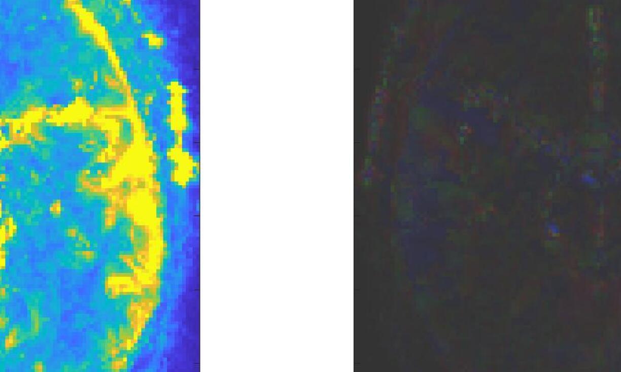
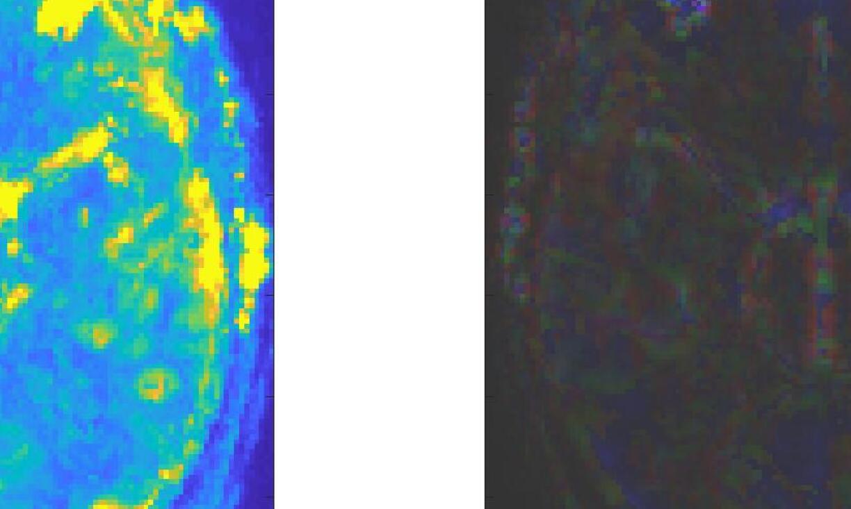
Figure 4.1: Results of our proposed algorithm applied to subject 2 (upper two figures) and subject 16 (lower two figures) of the data set. Velocity norm MIPs (left) and colour direction MIPs (right).

Figure 4.1 shows the results of our CGNE algorithm terminated after $10$ iterations, in the same way as in [10]. The left images in the figure show maximum intensity projections (MIPs) over the $z$-axis of the norm of the reconstructed PWV vector field $v$. One can clearly see the location of some of the major blood vessels as well as (relative) information on the absolute velocity of the PWV. The right images show colour direction MIPs, created by assigning an RGB value to every pixel of the MIP by first identifying the voxel whose velocity norm entered the MIP at that pixel, and then taking the absolute values of the components $v_{1}$, $v_{2}$, and $v_{3}$ of the PWV at that voxel as the red, green, and blue values of the RGB triplet at that pixel, respectively. For example, a red pixel in the colour direction MIP indicates movement along the $x$-axis, a green pixel along the $y$-axis and a blue pixel along the $z$-axis. uniform scaling was applied to the resulting figures to enhance their colours. From this one can get some idea about the direction of the PWV.

From a visual comparison with the results in [25, 10], one can see that our CGNE approach yields much better results than the one proposed in [25]and leads to similar results as the algorithm proposed in [10]. However, it is much faster than the iterative algorithm from [10], requiring only around $4$ instead of $14$ s per iteration on the same workstation (Intel(R) Xeon(R) CPU E5-1620 v4 @3.50GHz). Furthermore, it also scales much better with respect to the size of the input, as all calculations are explicit and no matrices need to be assembled or stored. This difference in speed makes it possible to process MRI data sets with a much higher spatio-temporal resolution.

5 Conclusion and Outlook

In this paper we proposed a CGNE-based algorithm for solving the parameter estimation problem of MRAI. Based on a reformulation of the problem as a linear operator equation with both a noisy operator and a noisy right-hand side, this algorithm allows for an efficient numerical implementation which can also handle MRI data sets with a high spatio-temporal resolution, which will be available in the near future. Numerical experiments on experimental data show the competitiveness of our algorithm in comparison with existing reconstruction algorithms.

6 Support

S. Hubmer and R. Ramlau were (partly) funded by the Austrian Science Fund (FWF): F6805-N36, project 5 and W1214-N15, project DK8.

H. Voss acknowledges support by the Nancy M. and Samuel C. Fleming Research Scholar Award in Intercampus Collaborations, Cornell University.

References

- [1] H. G. Bogren, R. H. Mohiaddin, R. K. Klipstein, D. N. Firmin, R. S. Underwood, S. R. Rees, and D. B. Longmore. The function of the aorta in ischemic heart-disease - a magnetic-resonance and angiographic study of aortic compliance and blood-flow patterns. American Heart Journal, 118(2):234–247, 1989.
- [2] P. Boutouyrie, S. Vermersch, S. Laurent, and M. Briet. Cardiovascular risk assessment through target organ damage: Role of carotid to femoral pulse wave velocity. Clinical and Experimental Pharmacology and Physiology, 35(4):530–533, 2008.
- [3] J. C. Bramwell. The velocity of the pulse wave in man. Proceedings of the Royal Society of London Series B-Containing Papers of a Biological Character, 93(652):298–306, 1922.
- [4] P. Elter. Methoden und Systeme zur nichtinvasiven, kontinuierlichen und belastungsfreien Blutdruckmessung. Thesis, Karlsruher Institut für Technologie, 2001.
- [5] H. W. Engl, M. Hanke, and A. Neubauer. Regularization of inverse problems. Dordrecht: Kluwer Academic Publishers, 1996.
- [6] A. C. Guyton and J. E. Hall. Textbook of Medical Physiology. Saunders/Elsevier, Philadelphia, Pa., 11th edition, 2006.
- [7] M. Hanke, F. J. Baumgartner, P. Ibe, F. R. Kaule, S. Pollmann, O. Speck, W. Zinke, and J. Stadler. A high-resolution 7-Tesla fMRI dataset from complex natural stimulation with an audio movie. Scientific Data, 1:140003:1–18, 2014.
- [8] B. Heintz, T. Gillessen, F. Walkenhorst, J. V. Dahl, R. Dorr, W. Krebs, P. Hanrath, and H. G. Sieberth. Evaluation of segmental elastic properties of the aorta in normotensive and medically treated hypertensive patients by intravascular ultrasound. Journal of Hypertension, 11(12):1253, 1993.
- [9] T. Honda, K. Yano, H. Matsuoka, M. Hamada, and K. Hiwada. Evaluation of aortic distensibility in patients with essential-hypertension by using cine magnetic-resonance-imaging. Angiology, 45(3):207–211, 1994.
- [10] S. Hubmer, A. Neubauer, R. Ramlau, and H. U. Voss. On the parameter estimation problem of magnetic resonance advection imaging. Inverse Problems and Imaging, 12(1):175–204, 2018.
- [11] D. J. Korteweg. Über die fortpflanzungsgeschwindigkeit des schalles in elastischen röhren. Annalen der Physik, 241(12):525–542, 1878.
- [12] M. Kozakova, C. Morizzo, D. Guarino, G. Federico, M. Miccoli, C. Giannattasio, and C. Palombo. The impact of age and risk factors on carotid and carotid-femoral pulse wave velocity. Journal of Hypertension, 33(7):1446–1451, 2015.
- [13] S. Laurent, J. Cockcroft, L. Van Bortel, P. Boutouyrie, C. Giannattasio, D. Hayoz, B. Pannier, C. Vlachopoulos, I. Wilkinson, H. Struijker-Boudier, and European Network Non-invasive. Expert consensus document on arterial stiffness: Methodological issues and clinical applications. European Heart Journal, 27(21):2588–2605, 2006.
- [14] J. K. J. Li. Dynamics of the Vascular System. Series on Bioengineering and Biomedical Engineering. World Scientific, River Edge, N.J., 2004.
- [15] C. K. Macgowan, S. J. Stoops, Y. Q. Zhou, L. S. Cahil, and J. G. Sled. Evaluation of cerebrovascular impedance and wave reflection in mouse by ultrasound. Journal of Cerebral Blood Flow and Metabolsim, 35(3):521–6, 2015.
- [16] G. Mancia. 2007 Guidelines for the Management of Arterial Hypertension: The task force for the management of arterial hypertension of the European Society of Hypertension and of the European Society of Cardiology. Journal of Hypertension, 25(8):1749–1749, 2007.
- [17] F. U. S. Mattace-Raso, A. Hofman, G. C. Verwoert, J. C. M. Witteman, I. Wilkinson, J. Cockcroft, C. McEniery, Yasmin, S. Laurent, P. Boutouyrie, E. Bozec, T. W. Hansen, C. Torp-Pedersen, H. Ibsen, J. Jeppesen, S. J. Vermeersch, E. Rietzschel, M. De Buyzere, T. C. Gillebert, L. Van Bortel, P. Segers, C. Vlachopoulos, C. Aznaouridis, C. Stefanadis, A. Benetos, C. Labat, P. Lacolley, C. D. A. Stehouwer, G. Nijpels, J. M. Dekker I. Ferreira, J. W. R. Twisk, S. Czernichow, P. Galan, S. Hercberg, B. Pannier, A. Guerin, G. London, J. K. Cruickshank, S. G. Anderson, A. Paini, E. A. Rosei, M. L. Muiesan, M. Salvetti, J. Filipovsky, J. Seidlerova, and M. Dolejsova. Determinants of pulse wave velocity in healthy people and in the presence of cardiovascular risk factors: “establishing normal and reference values”. European Heart Journal, 31(19):2338–2350, 2010.
- [18] C. M. McEniery, Yasmin, I. R. Hall, A. Qasem, I. B. Wilkinson, J. R. Cockcroft, and ACCT Investigators. Normal vascular aging: Differential effects on wave reflection and aortic pulse wave velocity - The Anglo-Cardiff Collaborative Trial (ACCT). Journal of the American College of Cardiology, 46(9):1753–1760, 2005.
- [19] S. Meaume, A. Benetos, O. F. Henry, A. Rudnichi, and M. E. Safar. Aortic pulse wave velocity predicts cardiovascular mortality in subjects ¿ 70 years of age. Arteriosclerosis Thrombosis and Vascular Biology, 21(12):2046–2050, 2001.
- [20] A. I. Moens. Over de voortplantingssnelheid van den pols [On the speed of propagation of the pulse]. PhD thesis, University of Leiden, Leiden, The Netherlands, 1877.
- [21] R. H. Mohiaddin, D. N. Firmin, and D. B. Longmore. Age-related-changes of human aortic flow wave velocity measured noninvasively by magnetic-resonance-imaging. Journal of Applied Physiology, 74(1):492–497, 1993.
- [22] S. Ogawa, T. M. Lee, A. R. Kay, and D. W. Tank. Brain magnetic-resonance-imaging with contrast dependent on blood oxygenation. Proceedings of the National Academy of Sciences of the United States of America, 87(24):9868–9872, 1990.
- [23] W. J. Rogers, Y. L. Hu, D. Coast, D. A. Vido, C. M. Kramer, R. E. Pyeritz, and N. Reichek. Age-associated changes in regional aortic pulse wave velocity. Journal of the American College of Cardiology, 38(4):1123–1129, 2001.
- [24] M. K. Stehling, R. Turner, and P. Mansfield. Echo-planar imaging - magnetic-resonance-imaging in a fraction of a second. Science, 254(5028):43–50, 1991.
- [25] H. U. Voss, J. P. Dyke, K. Tabelow, N. D. Schiff, and D. J. Ballon. Magnetic resonance advection imaging (MRAI) of cerebrovascular pulse dynamics. Journal of Cerebral Blood Flow and Metabolism, 37:1223 – 1235, 2017.
- [26] Z. Vrselja, H. Brkic, S. Mrdenovic, R. Radic, and G. Curic. Function of circle of Willis. Journal of Cerebral Blood Flow and Metabolism, 34(4):578–84, 2014.
- [27] S. Vulliemoz, N. Stergiopulos, and R. Meuli. Estimation of local aortic elastic properties with MRI. Magnetic Resonance in Medicine, 47(4):649–654, 2002.
- [28] A. L. Wentland, T. M. Grist, and O. Wieben. Review of MRI-based measurements of pulse wave velocity: a biomarker of arterial stiffness. Cardiovasc Diagn Ther, 4(2):193–206, 2014.