The Fast and the Flexible: training neural networks to learn to follow instructions from small data

Abstract

Learning to follow human instructions is a long-pursued goal in artificial intelligence. The task becomes particularly challenging if no prior knowledge of the employed language is assumed while relying only on a handful of examples to learn from. Work in the past has relied on hand-coded components or manually engineered features to provide strong inductive biases that make learning in such situations possible. In contrast, here we seek to establish whether this knowledge can be acquired automatically by a neural network system through a two phase training procedure: A (slow) offline learning stage where the network learns about the general structure of the task and a (fast) online adaptation phase where the network learns the language of a new given speaker. Controlled experiments show that when the network is exposed to familiar instructions but containing novel words, the model adapts very efficiently to the new vocabulary. Moreover, even for human speakers whose language usage can depart significantly from our artificial training language, our network can still make use of its automatically acquired inductive bias to learn to follow instructions more effectively.

1 Introduction

Learning to follow instructions from human speakers is a long-pursued goal in artificial intelligence, tracing back at least to Terry Winograd’s work on SHRDLU (Winograd, 1972). This system was capable of interpreting and following natural language instructions about a world composed of geometric figures. While this first system relied on a set of hand-coded rules to process natural language, most of recent work aimed at using machine learning to map linguistic utterances into their semantic interpretations (Chen and Mooney, 2011; Artzi and Zettlemoyer, 2013; Andreas and Klein, 2015). Predominantly, they assumed that users speak all in the same natural language, and thus the systems could be trained offline once and for all. However, recently Wang et al. (2016) departed from this assumption by proposing SHRDLURN, a coloured-blocks manipulation language game. There, users could issue instructions in any arbitrary language to a system that must incrementally learn to interpret it (see Figure 1 for an example). This learning problem is particularly challenging because human users typically provide only a handful of examples for the system to learn from. Therefore, the learning algorithms must incorporate strong inductive biases in order to learn effectively. That is, they need to complement the scarce input with priors that would help the model make the right inferences even in the absence of positive data. A way of giving the models a powerful inductive bias is by hand-coding features or operations that are specific to the given domain where the instructions must be interpreted. For example, Wang et al. (2016) propose a log-linear semantic parser which crucially relies on a set of hand-coded functional primitives. While effective, this strategy severely curtails the portability of a system: For every new domain, human technical expertise is required to adapt the system. Instead, we would like these inductive biases to be learned automatically without human intervention. That is, humans should be free from the burden of thinking what are useful primitives for a given domain, but still obtain systems that can learn fast from little data.

Figure 1: Illustration of the SHRDLURN task of Wang et al. (2016)

In this paper, we introduce a neural network system that learns domain-specific priors directly from data. This system can then be used to quickly learn the language of new users online. It uses a two phase regime: First, the network is trained offline on easy-to-produce artificial data to learn the mechanics of a given task. Next, the network is deployed to real human users who will train it online with just a handful of examples. While this implies that some of the manual effort needed to design useful primitive functions would go in developing the artificial data, we envision that in many real-world situations it could be easier to provide examples of expected interactions than thinking of what could be useful primitives involved in them. On controlled experiments we show that our system can recover the meaning of sentences where some words where scrambled, even though it does not display evidence of compositional learning. On the other hand, we show that the offline training phase allows it to learn faster from limited data, compared to a neural network system that did not go through this pre-training phase. We hypothesize that this system learns useful inductive biases, such as the types of operations that are likely to be requested. In this direction, we show that the performance of our best-performing system correlates with that of Wang et al., where these operations were encoded by hand.

The work in this paper is organized as follows: We first start by creating a large artificially generated dataset to train the systems in the offline phase. We then experiment with different neural network architectures to find which general learning system adapts best for this task. Then, we propose how to adapt this network by training it online and confirm its effectiveness on recovering the meaning of scrambled words and on learning to process the language from human users, using the dataset introduced by Wang et al. (2016).

2 Related Work

Learning to follow human natural language instructions has a long tradition in NLP, dating at least back to the work of Terry Winograd Winograd (1972), who developed a rule-based system for this endeavour. Subsequent work centered around automatically learning the rules to process language (Shimizu and Haas, 2009; Chen and Mooney, 2011; Artzi and Zettlemoyer, 2013; Vogel and Jurafsky, 2010; Andreas and Klein, 2015). This line of work assumes that users speak all in the same language, and thus a system can be trained on a set of dialogs pertaining to some of those speakers and then generalize to new ones. Instead, Wang et al. (2016) describe a block manipulation game in which a system needs to learn to follow natural language instructions produced by human users using the correct outcome of the instruction as feedback. What distinguishes this from other work is that every user can speak in their own –natural or invented– language. For the game to remain engaging, the system needs to quickly adapt to the user’s language, thus requiring a system that can learn much faster from small data. The system they propose is composed of a set of hand-coded primitives (e.g., remove, red, with) that can manipulate the state of the block piles and a log-linear learning model that learns to map n-gram features from the linguistic instructions (like, for instance, ‘remove red’) to expressions in this programming language (e.g., remove(with(red))). Our work departs from this base in that we provide no hand-coded primitives to solve this task, but aim at learning an end-to-end system that follows natural language instructions from human feedback. Another line of research that is closely related to ours, is that of fast mapping (Lake et al., 2011; Trueswell et al., 2013; Herbelot and Baroni, 2017), where the goal is to acquire a new concept from a single example of its usage in context. While we don’t aim at learning new concepts here, we do want to learn from few examples to draw an analogy between a new term and a previously acquired concept. Finally, our work can be seen as an instance of the transfer learning paradigm (Pan and Yang, 2010), which has been successful in both linguistic (Mikolov et al., 2013; Peters et al., 2018) and visual processing (Oquab et al., 2014). Rather than transferring knowledge from one task to another, we are transferring between artificial and natural data.

3 Method

A model aimed at following natural language instructions must master at least two skills. First, it needs to process the language of the human user. Second, it must act on the target domain in sensible ways (and not trying actions that a human user would probably never ask for). Whereas the first aspect is dependent on each specific user’s language, the second requirement is not related to a specific user, and could – as illustrated by the successes of Wang et al.’s log-linear model – be learned beforehand. To allow a system to acquire these skills automatically from data, we introduce a two-step training regime. First, we train the neural network model offline on a dataset that mimics the target task. Next, we allow this model to independently adapt to the language of each particular human user by training it online with the examples that each user provides.

3.1 Offline learning phase

The task at hand is, given a list of piles of coloured blocks and a natural language instruction, to produce a new list of piles that matches the request. The first step of our method involves training a neural network model to perform this task. We used supervised learning to train the system on a dataset that we constructed by simulating a user playing the game. In this way, we did not require any real data to kick-start our model. Below we describe, first, the procedure used to generate the dataset and, second, the neural network models that were explored in this phase.

Data

The data for SHRDLURN task takes the form of triples: a start configuration of colored blocks grouped into piles, a natural language instruction given by a user and the resulting configuration of colored blocks that comply with the given instruction (Figure 1). We generated 88 natural language instructions following the grammar in Figure 2(a). The language of the grammar was kept as minimal as possible, with just enough variation to capture the simplest possible actions in this game. Furthermore, we sampled as many as needed initial block configurations by building 6 piles containing a maximum of 3 randomly sampled colored blocks each. The piles in the dataset were serialized into a sequence by encoding them into 6 lists delimited by a special symbol, each of them containing a sequence of color tokens or a special empty symbol. We then computed the resulting target configuration using a rule-based interpretation of our grammar. An example of our generated data is depicted in Figure 2(b).

S	$\rightarrow$	VERB COLOR at POS tile
VERB	$\rightarrow$	add $|$ remove
COLOR	$\rightarrow$	red $|$ cyan $|$ brown $|$ orange
POS	$\rightarrow$	1st $|$ 2nd $|$ 3rd $|$ 4th $|$
		5th $|$ 6th $|$ even $|$ odd $|$
		leftmost $|$ rightmost $|$ every

(a) Grammar of our artificially generated language

Instruction	remove red at 3rd tile
Initial Config.	BROWN X X # RED X X # ORANGE RED X
Target Config.	BROWN X X # RED X X # ORANGE X X

(b) Example of an entry in our dataset. We show three rather than six columns for conciseness.

Figure 2: Artificially generated data

Model

To model this task we used an encoder-decoder (Sutskever et al., 2014) architecture: The encoder reads the natural language utterance $\mathbf{w}=w_{1},\dots,w_{m}$ and transforms it into a sequence of feature vectors $\mathbf{h_{1}},\dots,\mathbf{h}_{m}$, which are then read by the decoder through an attention layer. This latter module reads the sequence describing the input block configurations $\mathbf{x}=x_{1},\dots,x_{n}$ and produces a new sequence $\mathbf{\hat{y}}=\hat{y}_{1},\dots,\hat{y}_{n}$ that is construed as the resulting block configuration. To pass information from the encoder to the decoder, we equipped the decoder with an attention mechanism (Bahdanau et al., 2014; Luong et al., 2015). This allows the decoder, at every timestep, to extract a convex combination of the hidden vectors $\mathbf{h}$. We trained the system parameters $\theta=(\theta_{\text{enc}},\theta_{\text{dec}})$ so that the output matches the target block configuration $\mathbf{y}=y_{1},\dots,y_{n}$ (represented as 1-hot vectors) using a cross-entropy loss:

$$\mathbf{h} =\operatorname{encoder}_{\theta_{\text{enc}}}(\mathbf{w})$$

$$\mathbf{\hat{y}} =\operatorname{decoder}_{\theta_{\text{dec}}}(\mathbf{x}|\mathbf{h})$$

$$\mathcal{L}(\mathbf{y},\mathbf{\hat{y}}) =\sum_{i=1}^{n}y_{i}\log\hat{y}_{i}$$

Both the encoder and decoder modules are sequence models, meaning that they read a sequence of inputs and compute, in turn, a sequence of outputs, and that can be trained end-to-end. We experimented with two state-of-the-art sequence models: A standard recurrent LSTM (Hochreiter and Schmidhuber, 1997) and a convolutional sequence model (Gehring et al., 2016; Gehring et al., 2017), which has been shown to outperform the former on a range of different tasks (Bai et al., 2018). For the convolutional model we used kernel size $k=3$ and padding to make the size of the output match the size of the input sequence. Because of the invariant structure of the block configuration that is organized into lists of columns, we expected the convolutional model (as a decoder) to be particularly well-fit to process them. We explored all possible combinations of architectures for the encoder and decoder components. Furthermore, as a simple baseline, we also considered a bag-of-words encoder that computes the average of trainable word embeddings.

3.2 Online learning phase

Once the model has been trained to follow a specific set of instructions given by a simulated user, we want it to serve a new, real user, who does not know anything about how the model was trained and is encouraged to communicate with the system using her own language. To do so, the model will have to adapt to follow instructions given in a potentially very different language from the one it has seen during offline training. One of the first challenges it will encounter is to quickly master the meaning of new words. This challenge of inferring the meaning of a word from a single exposure goes by the name of ‘fast-mapping’ (Lake et al., 2011; Trueswell et al., 2013). Here, we take inspiration from the method proposed by Herbelot and Baroni (2017), who learn the embeddings for new words with gradient descent, freezing all the other network weights. We further develop it by experimenting with different variations of this method: Like them, we try learning only new word embeddings, but also learning the full embedding layer (thus allowing words seen during offline training to shift their meaning). Additionally, we test what happens when the full encoder weights are unfrozen, allowing to adapt not only the embeddings but also how they are processed sequentially. In the latter two cases, we incorporate $L_{2}$ regularization over the embeddings and the model weights.

Human users interact with the system by asking it in their own language to perform transformations on the colored block piles, providing immediate feedback on what was the intended target configuration. In our system, each new example that the model observes is added to a buffer $B$. Then, the model is further trained with a fixed number of gradient descent steps $S$ on predicting the correct output using examples randomly drawn from a subset $B_{\text{TR}}\subseteq B$ of this buffer.

In order to reduce the impact of local minima that the model could encounter when learning from just a handful of examples, we train $k$ different copies (rather than training a single model) each with a set of differently initialized embeddings for new words. In this way, we can pick the best model to make a future prediction, not only based on how well it has fitted previously seen data, but also by how well it generalizes to other examples. For choosing which model to use, we use a different (not necessarily disjoint) subset of examples called $B_{\text{VA}}\subseteq B$. We experimented with two model selection strategies: greedy, by which we pick the model with the lowest loss computed over the full training buffer examples ($B_{\text{VA}}=B_{\text{TR}}=B$); and 1-out, where we save the last example for validation and pick the model that has the lowest loss on that example ($B_{\text{VA}}=B[\texttt{LAST}]$, $B_{\text{TR}}=B[0:\texttt{LAST}-1]$) . Algorithm 1 summarizes our approach.

Algorithm 1 Online Training

1:Initialize models $m_{1},\dots,m_{k}$

2:Let $B$ be an empty training buffer

3:for t = 1,2,…,T do

4:    Observe the input utterance $\mathbf{w}_{t}$ and block configuration $\mathbf{x}_{t}$

5:    Select best model $m_{i}$ using data $B_{\text{VA}}$

6:    Predict $\hat{\mathbf{y}_{t}}=m_{i}(\mathbf{w}_{t},\mathbf{x}_{t})$

7:    Observe feedback $\mathbf{y}_{t}$.

8:    Record prediction accuracy ($\mathbf{y}_{t}==\hat{\mathbf{y}}_{t}$)

9:    Add $(\mathbf{w}_{t},\mathbf{x}_{t},\mathbf{y}_{t})$ to $B$

10:    Train $m_{1},\dots,m_{k}$ on data $B_{\text{TR}}$

11:procedure Select($m_{1},\dots,m_{k}$, $B_{\text{VA}}$)

12:    Let $C_{i}\leftarrow\sum_{\mathbf{(\mathbf{w},\mathbf{x},\mathbf{y})}\in B_{\text{VA}}}{\mathcal{L}(\mathbf{y},m_{i}(\mathbf{w},\mathbf{x}))}$

13:    return $m_{i}$ having minimal $C_{i}$

14:procedure Train($m_{1},\dots,m_{k}$, $B_{\text{TR}}$)

15:    for $i=1,\dots,k$, $s=1,\dots,S$ do

16:         Draw $\mathbf{w},\mathbf{x},\mathbf{y}\sim B_{\text{TR}}$

17:         Predict $\hat{\mathbf{y}_{t}}=m_{i}(\mathbf{w}_{t},\mathbf{x}_{t})$

18:         Compute $\nabla_{\theta_{i}}\mathcal{L}(\mathbf{y},\hat{\mathbf{y}_{t}})$

19:         Update $m_{i}$ by a gradient step on $\theta_{i}$     

4 Experiments

We seek to establish whether we can train a neural network system to learn the rules and structure of a task while communicating with a scripted teacher and then having it adapt to the particular nuances of each human user. We tackled this question incrementally. First, we explored what is the best architectural choice for solving the SHRDLURN task on our large artificially-constructed dataset. Next, we ran multiple controlled experiments to investigate the adaptation skills of our online learning system. In particular, we first tested whether the model was able to recover the original meaning of a word that had been replaced with a new arbitrary symbol – e.g. “red” becomes “roze”– on an online training regime. Finally, we proceeded to learn from real human utterances using the dataset collected by Wang et al. (2016).

4.1 Offline training

We used the data generation method described in the previous section to construct a dataset to train our neural network systems. To evaluate the models in a challenging compositional setting, rather than producing a random split of the data, we create validation and test sets that have no overlap with training instructions or block configurations. To this end, we split all the 88 possible utterances that can be generated from our grammar into 66 utterances for training, 11 for validation and 11 for testing. Similarly, we split all possible 85 combinations that make a valid column of blocks into 69 combinations for training, 8 for validation and 8 for testing, sampling input block configurations using combinations of 6 columns pertaining only to the relevant set. In this way, we generated 42000 instances for training, 4000 for validation and 4000 for testing.

We explored all possible combinations of encoder and decoder models: LSTM encoder and LSTM decoder (seq2seq), LSTM encoder and convolutional decoder (seq2conv), convolutional encoder and LSTM decoder (conv2seq), and both convolutional encoder and decoder (conv2conv). Furthermore, we explored a bag of words encoder with an LSTM decoder (bow2seq). We trained 5 models with our generated dataset and use the best performing for the following experiments. We conducted a hyperparameter search for all these models, exploring the number of layers (1 or 2 for LSTMs, 4 or 5 for the convolutional network), the size of the hidden layer (32, 64, 128, 256) and dropout rate (0, 0.2, 0.5). For each model, we picked the hyperparameters that maximized accuracy on our validation set and report validation and test accuracy in Table 1.

As it can be noticed, seq2conv is the best model for this task by a large margin, performing perfectly or almost perfectly on this challenging test split featuring only unseen utterances and block configurations. Furthermore, this validates our hypothesis that the convolutional decoder is better fitted to process the structure of the block piles.

Model	Val. Accuracy	Test Accuracy
seq2seq	$78$	$79$
seq2conv	$\mathbf{99}$	$\mathbf{100}$
conv2seq	$73$	$67$
conv2conv	$64$	$74$
bow2seq	$57$	$63$

Table 1: Model’s accuracies (in percentages) evaluated on block configurations and utterances that were completely unseen during offline training. Results expressed in percentages.

4.2 Recovering corrupted words

Next, we ask whether our system could adapt quickly to controlled variations in the language. To test this, we presented the model with a simulated user producing utterances drawn from the same grammar as before, but where some words have been systematically corrupted so the model cannot recognize them anymore. We then evaluated the model on whether it can recover the meaning of these words during online training. For this experiment, we combined the validation and test sections of our dataset, containing in all 22 different utterances, to make sure that the presented utterances were completely unseen during training time. We then split the vocabulary in two disjoint sets of words that we want to corrupt, one for validation and one for testing. For validation, we take one verb (“add”), 2 colors (“orange” and “red”), and 4 positions (“1st”, “3rd; ; “5th” and “even”), keeping the remaining alternatives for testing. We then extracted a set of 15 utterances containing these words and corrupted each occurrence of them by replacing them with a new token (consistently keeping the same new token for each occurrence of the word). In this way, we obtained a validation set where we can calibrate hyper-parameters for all the test conditions that we describe below. We further extracted, for each of these utterances, 3 block configurations to pair them with, resulting in a simulated session with 45 instruction examples. For testing, we created controlled sessions where we corrupted: one single word, two words of different type (e.g. verb and color), three words of different types and finally, all words from the test set vocabulary. Each condition allows for different a number of sessions because of the number of ways one can chose words from these sets. By keeping the two vocabularies disjoint we make sure that by optimizing the hyperparameters of our online training scheme, we don’t happen to be good at recovering words from a particular subset.

We use the validation set to calibrate the hyperparameters of the online training routine. In particular, we vary the optimization algorithm to use (Adam or SGD), the number of training steps (100, 200 or 500), the regularization weight ($0$, $10^{-2}$, $10^{-3}$, $10^{-4}$), the learning rate ($10^{-1}$, $10^{-2}$, $10^{-3}$), and the model selection strategy (greedy or 1-out), while keeping the number of model parameters that are trained in parallel fixed to $k=7$. For this particular experiment, we considered learning only the embeddings for the new words, leaving all the remaining weights frozen (model 1). To assess the relative merits of this model, we compared it with ablated versions where the encoder has been randomly initialized but the decoder is kept fixed (model 2) and a fully randomly initialized model (model 3). Furthermore, we evaluated the impact of having multiple ($k=7$) concurrently trained model parameters by comparing it with just having a single set of parameters trained (model 4). We report the best hyperparameters for each model in the supplementary materials. We use online accuracy as our figure of merit, computed as $\frac{1}{T}\sum_{t=1}^{T}{\mathbb{I}[\mathbf{\hat{y}}_{t}==\mathbf{y}_{t}]}$, where $T$ is the length of the session. We report the results in Table 2.

			N. of corrupted words
	Transfer	Adapt	1	2	3	all
$k=7$
1.	Enc+Dec	Emb.	$90.9$	$\mathbf{88.1}$	$\mathbf{86.1}$	$\mathbf{73.3}$
2.	Dec.	Enc.	$\mathbf{93.8}$	$85.9$	$82.4$	$55.5$
3.	$\emptyset$	Enc + Dec	$43.3$	$35.5$	$36.1$	$36.7$
$k=1$
4.	Enc+Dec	Emb.	$86.1$	$84.3$	$81.8$	$55$

Table 2: Online accuracies (in percentages) for the word recovery task averaged over 7 sessions for 1 word, 17 for 2 words, 10 for 3 words and a single interaction for the all words condition, having 45 instructions each. “Transfer” stands for the components whose weights were saved (and not reinitialized) from the offline training. “Adapt” stands for the components whose weights get updated during the online training.

First, we can see that –perhaps not too surprisingly– the model that adapts only the word embeddings performs best overall. Notably, it can reach 73% accuracy even when all words have been corrupted (whereas, for example, the model of Wang et al. (2016) obtains 55% on the same task). The only exception comes in the single corrupted word condition, where re-learning the full encoder seems to be performing even better. A possible explanation is given by the discrepancy between this condition and the validation set, which was more akin to the “all” condition, resulting in suboptimal hyperparameters for the condition with a single word changed. Nevertheless, it is encouraging to see that the model can quickly learn to perform the instructions even in the most challenging setting where all words have been changed. In addition, we can observe the usefulness of having multiple sets of parameters trained, by comparing the “Embeddings” models by default trained with $k=7$ models and when $k=1$, noting that the former is consistently better.

4.3 Adapting to human speakers

Having established our model’s ability to recover the meaning of masked known concepts, albeit in similar contexts as those seen seen during training, we moved to the more challenging setting where the model needs to adapt to real human speakers. In this case, the language can significantly depart from the one seen during the offline learning phase, both in surface form and in their underlying semantics. For these experiments we used the dataset made available by Wang et al. (2016), collected from turkers playing SHRDLURN in collaboration with their log-linear/symbolic model. The dataset contains 100 sessions with nearly 8k instruction examples. We first selected three sessions in this dataset to produce a validation set to tune the online learning hyperparameters. All the remaining 97 sessions were left for testing. In order to assess the relative importance of our pre-training procedure on each of our model’s components, we explored 6 different variants of our model. On one hand, we varied which set of pre-trained weights were kept without reinitializing them: (a) All the weights in the encoder plus all the weights of the decoder; (b) only the decoder weights while randomly initializing the encoder; or (c) no weights and thus, resetting them all (this taking the role of a baseline for our method). On the other hand, we explored which subset of weights we adapt, leaving all the rest frozen: (1) Only the word embeddings, (2) the full weights of the encoder or (3) the full network (both encoder and decoder). Among the 9 possible combinations, we restricted to the 6 that wouldn’t result on random components not being updated (for example (c-2) would result in a model with a randomly initialized decoder that is never trained), thus leaving out (c-1), (c-2) and (b-1). For each of the remaining 6 valid training regimes, we ran an independent hyperparameter search choosing from the same pool of candidate values as in the word recovery task (see Section 4.2). We picked the hyperparameter configuration that maximized the average online accuracy on the three validation sessions. The best hyperparameters are reported on the supplementary materials.

		Adapt
		(1) Embeddings		(2) Encoder		(3) Encoder+Decoder
		acc.	$r$	acc.	$r$	acc.	$r$
Reuse	(c) Nothing (Random)	-	-	-	-	$13.5$	$0.58$
	(b) Decoder (Random Encoder)	-	-	$\mathbf{23}$	$0.83$	$21$	$0.7$
	(a) Encoder + Decoder	$18.2$	$0.74$	$22.6$	$\mathbf{0.84}$	$21.3$	$0.72$

Table 3: For each (valid) combination of set of weights to re-use and weights to adapt online, we report average online accuracy on Wang et al. (2016) dataset and pearson-$r$ correlation between online accuracies obtained by our model and those reported by the author. Results obtained on 220 sessions, with about 39 $\pm$ 31 interactions each.

.

We then evaluated each of the model variants on the 97 interactions in our test set using average online accuracy as figure of merit. Furthermore, we also computed the correlation between the online accuracy obtained by our model on every single session and that obtained by Wang et al.’s system which was endowed with hand-coded functions. The higher the correlation, the more our model behaves in a similar fashion to theirs, learning or failing to do so on the same sessions.

The results of these experiments are displayed in Table 3.

In the first place, we observe that models using knowledge acquired in the offline training phase (rows a and b) perform (in terms of accuracy) better than a randomly initialized model (c-3), confirming the effectiveness of our offline training phase. Second, a randomly initialized encoder with a fixed decoder (b-2) performs slightly better than the pre-trained one (a-2). This result suggests that the model is better off ignoring the specifics of our artificial grammar and learning the language from scratch, even from very few examples. Therefore, no manual effort is required to reflect the specific surface form of a user’s language when training the system offline on artificial data. Finally, we observe that the models that perform the best are those in column (2) which adapt the encoder weights and freeze the decoder ones. This is congruent to what would be expected if the decoder is implementing task-specific knowledge because the task has remained invariant between the two phases and thus, the components presumedly related to solving it should not need to change. Interestingly, variants in these column also correlate the most with the symbolic system. Moreover, performance scores seem to be strongly aligned with the correlation coefficients. As a matter of fact the 7 entries of online accuracy and pearson $r$ are themselves correlated with $r=0.99$, which is highly significant even for these few data points. This result is compatible with our hypothesis that the symbolic system carries learning biases which, the better our models are at capturing, the better they will perform in the end task. Still, evidence for our hypothesis, based both on the effectiveness of the pre-training step and on the fact that similar systems should succeed and fail on similar situations, is still indirect. We leave for future work the interesting question of through which mechanisms the decoder is implementing useful task-specific information, and whether they mimic the functions that are implemented in Wang et al.’s system, or whether they are of a different nature.

Furthermore, to test whether the model was harnessing similarities between our artificial and the human-produced data, we re-trained our model on our artificial dataset after scrambling all words and shuffling word order in all sentences in an arbitrary but consistent way, thus destroying any existing similarity at lexical or syntactic levels. Then, we repeated the online training procedure keeping the decoder weights, obtaining 20.7% mean online accuracy, which is much closer to the results of the models trained on the original grammar than it is to the randomly initialized model. With this, we conclude that a large part of the knowledge that the model exploits comes from the tasks mechanics than from specifics of the language used.

Finally, we note that the symbolic model attains a higher average online accuracy of $33\%$ in this dataset, showing that there is still room for improvement in this task. Yet, it is important to remark that since this model features hand-coded domain knowledge it is expected to have an advantage over a model that has to learn these rules from data alone, and thus the results are not directly comparable but rather serve as a reference point.

5 Analysis

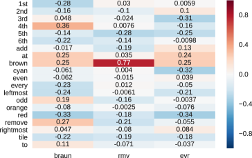
3a Cosine similarities of the newly learned word embedding for the corrupted version of the words “brown”, “remove” and “every” with the rest of the vocabulary.

3b Example of failing case for our system. During offline training it had not seen other colored blocks to be used as referring expressions for locations.

Word recovery

To gain some further understanding of what our model learns, we examined the word embeddings learned by our model in the word recovery task. In particular, we wanted to see whether the embedding that the model had re-learned for the corrupted word was similar to the embedding of the original word. We analyzed a session in which 3 words had been corrupted: “brown”, “remove” and “every”. Recall from Section 4.2 that these sessions are 45-interactions-long with 15 different utterances issued on 3 different inputs each. We then evaluated how close each of the corrupted versions of these words (called “braun”, “rmv” and “evr”) were to their original counterparts in terms of cosine similarity. Interestingly, the model performs very well, with an online accuracy of about 80%, with 50% of the errors concentrated on a single utterance that contains all corrupted words together: “rmv braun at evr tile”. However, as shown on Figure 3a, the system seems to be assigning most of the semantics associated to “brown” to the embedding for “rmv” (“brown” has much higher cosine similarity to “rmv” than to “braun”), implying that the system is confounding these two words. This is consistent with previous findings on machine learning systems (Sturm, 2014), showing that systems can easily learn some spurious correlation that fits the training data rather than the ground-truth generative process. Similar observations were brought forward on a linguistic context by Lake and Baroni (2017), where the authors show that, after a system has learned to perform a series of different instructions (e.g., “run”, “run twice”, “run left”), a new verb is taught to it (“jump”), but then it fails to generalize its usage to previously known contexts (“jump twice”, “jump left”). While our system seems to be capable of compositional processing, as suggested by the high accuracy on our compositional split shown in Section 4.1, it is not able to harness this structure during learning from few examples, as evidenced by this analysis. In other words, it is not capable of compositional learning. One possible route to alleviate this problem could include separating syntax and semantics as is customary on formal semantic methods (Partee et al., 1990) and, as recently suggested in the context of latent tree learning (Havrylov et al., 2019), so that syntax can guide semantics both in processing and learning.

Human data

On the previous section we have shown that the performance of our system correlates strongly with the symbolic system of Wang et al. Yet, this correlation is not perfect, and thus, there are sessions in which our system performs comparatively better or worse on a normalized scale. We looked for examples of such sessions in the dataset. Figure 3b shows a particular case that our system fails to learn. Notably it is using other blocks as referring expressions to indicate positions, a mechanism that the model had not seen during offline training, and thus it struggled to quickly assign a meaning to it.

On more realistic settings, language learning does not take the form of our idealized two-phase learning process, but it is an ongoing learning cycle where new communicative strategies can be proposed or discovered on the fly, as this example of using colors as referring expressions teaches us. Tackling this learning process requires advances that are well out of the scope of this work . However, we see these challenges as exciting problems to pursue in the future.

6 Conclusions

Learning to follow human instructions is a challenging task because humans typically (and rightfully so) provide very few examples to learn from. For learning from this data to be possible, it is necessary to make use of some inductive bias. Whereas work in the past has relied on hand-coded components or manually engineered features, here we sought to establish whether this knowledge can be acquired automatically by a neural network system through a two phase training procedure: A (slow) offline learning stage where the network learns about the general structure of the task and a (fast) online adaptation phase where the network needs to learn the language of a new specific speaker. Controlled experiments demonstrate that when the network is exposed to a language which is very similar to the one it has been trained on except for some new synonymous words, the model adapts very efficiently to the new vocabulary, albeit making non-compositional inferences. Moreover, even for human speakers whose language usage can considerably depart from our artificial language, our network can still make use of the inductive bias that has been automatically learned from the data to learn more efficiently. Interestingly, using a randomly initialized encoder on this task performs equally well or better than the pre-trained encoder, hinting that the knowledge that the network learns to re-use is more specific to the task rather than discovering language universals. This is not too surprising given the minimalism of our grammar.

To the best of our knowledge we are the first to present a neural model to play the SHRDLURN task without any hand-coded components. We believe that an interesting direction to explore in the future is adopting meta-learning techniques (Finn et al., 2017; Ravi and Larochelle, 2017), to tune the network parameters having in mind that they should serve for adaptation, or adopting syntax-aware models, which may improve sample efficiency for learning instructions. We hope that bringing together these techniques with the presented here, we can move closer to having fast and flexible human assistants.

References

- Andreas and Klein (2015) Andreas, J. and D. Klein (2015). Alignment-based compositional semantics for instruction following. In Proceedings of the 2015 Conference on Empirical Methods in Natural Language Processing (EMNLP), pp. 1165–1174.
- Artzi and Zettlemoyer (2013) Artzi, Y. and L. Zettlemoyer (2013). Weakly supervised learning of semantic parsers for mapping instructions to actions. Transactions of the Association of Computational Linguistics 1, 49–62.
- Bahdanau et al. (2014) Bahdanau, D., K. Cho, and Y. Bengio (2014). Neural machine translation by jointly learning to align and translate. In Proceedings of the 3rd International Conference on Learning Representations (ICLR2015).
- Bai et al. (2018) Bai, S., J. Z. Kolter, and V. Koltun (2018). An empirical evaluation of generic convolutional and recurrent networks for sequence modeling. CoRR abs/1803.01271.
- Chen and Mooney (2011) Chen, D. L. and R. J. Mooney (2011). Learning to interpret natural language navigation instructions from observations. In AAAI, Volume 2, pp. 1–2.
- Claeskens et al. (2008) Claeskens, G., N. L. Hjort, et al. (2008). Model selection and model averaging. Cambridge Books.
- Finn et al. (2017) Finn, C., P. Abbeel, and S. Levine (2017). Model-agnostic meta-learning for fast adaptation of deep networks. In International Conference on Machine Learning, pp. 1126–1135.
- Gehring et al. (2016) Gehring, J., M. Auli, D. Grangier, and Y. N. Dauphin (2016). A convolutional encoder model for neural machine translation. In Proceedings of the 55th Annual Meeting of the Association for Computational Linguistics (ACL), pp. 123–135.
- Gehring et al. (2017) Gehring, J., M. Auli, D. Grangier, D. Yarats, and Y. N. Dauphin (2017, 06–11 Aug). Convolutional sequence to sequence learning. In D. Precup and Y. W. Teh (Eds.), Proceedings of the 34th International Conference on Machine Learning, Volume 70 of Proceedings of Machine Learning Research, International Convention Centre, Sydney, Australia, pp. 1243–1252. PMLR.
- Havrylov et al. (2019) Havrylov, S., G. Kruszewski, and A. Joulin (2019). Cooperative learning of disjoint syntax and semantics. Proceedings of NAACL 2019.
- Herbelot and Baroni (2017) Herbelot, A. and M. Baroni (2017). High-risk learning: acquiring new word vectors from tiny data. In Proceedings of the 2017 Conference on Empirical Methods in Natural Language Processing, pp. 304–309.
- Hochreiter and Schmidhuber (1997) Hochreiter, S. and J. Schmidhuber (1997, November). Long short-term memory. Neural Computation 9(8), 1735–1780.
- Lake et al. (2011) Lake, B., R. Salakhutdinov, J. Gross, and J. Tenenbaum (2011). One shot learning of simple visual concepts. In Proceedings of the Annual Meeting of the Cognitive Science Society, Volume 33.
- Lake and Baroni (2017) Lake, B. M. and M. Baroni (2017). Still not systematic after all these years: On the compositional skills of sequence-to-sequence recurrent networks. CoRR abs/1711.00350.
- Luong et al. (2015) Luong, M., H. Pham, and C. D. Manning (2015, September). Effective approaches to attention-based neural machine translation. In Proceedings of the 2015 Conference on Empirical Methods in Natural Language Processing, Lisbon, Portugal, pp. 1412–1421. Association for Computational Linguistics.
- Mikolov et al. (2013) Mikolov, T., I. Sutskever, K. Chen, G. S. Corrado, and J. Dean (2013). Distributed representations of words and phrases and their compositionality. In Advances in neural information processing systems (NIPS), pp. 3111–3119.
- Oquab et al. (2014) Oquab, M., L. Bottou, I. Laptev, and J. Sivic (2014). Learning and transferring mid-level image representations using convolutional neural networks. In Computer Vision and Pattern Recognition (CVPR), 2014 IEEE Conference on, pp. 1717–1724. IEEE.
- Pan and Yang (2010) Pan, S. J. and Q. Yang (2010). A survey on transfer learning. IEEE Transactions on knowledge and data engineering 22(10), 1345–1359.
- Partee et al. (1990) Partee, B. B., A. G. ter Meulen, and R. Wall (1990). Mathematical methods in linguistics, Volume 30. Springer Science & Business Media.
- Peters et al. (2018) Peters, M. E., M. Neumann, M. Iyyer, M. Gardner, C. Clark, K. Lee, and L. Zettlemoyer (2018). Deep contextualized word representations. Proceedings of NAACL 2018.
- Ravi and Larochelle (2017) Ravi, S. and H. Larochelle (2017). Optimization as a model for few-shot learning. In Proceedings of the International Conference of Learning Representations(ICLR).
- Shimizu and Haas (2009) Shimizu, N. and A. R. Haas (2009). Learning to follow navigational route instructions. In IJCAI, Volume 9, pp. 1488–1493.
- Sturm (2014) Sturm, B. L. (2014). A simple method to determine if a music information retrieval system is a “horse”. IEEE Transactions on Multimedia 16(6), 1636–1644.
- Sutskever et al. (2014) Sutskever, I., O. Vinyals, and Q. V. Le (2014). Sequence to sequence learning with neural networks. In Advances in neural information processing systems (NIPS), pp. 3104–3112.
- Trueswell et al. (2013) Trueswell, J. C., T. N. Medina, A. Hafri, and L. R. Gleitman (2013). Propose but verify: Fast mapping meets cross-situational word learning. Cognitive psychology 66(1), 126–156.
- Vogel and Jurafsky (2010) Vogel, A. and D. Jurafsky (2010). Learning to follow navigational directions. In Proceedings of the 48th Annual Meeting of the Association for Computational Linguistics, pp. 806–814. Association for Computational Linguistics.
- Wang et al. (2016) Wang, S. I., P. Liang, and C. D. Manning (2016). Learning language games through interaction. In Proceedings of the 54th Annual Meeting of the Association for Computational Linguistics (ACL), pp. 2368–2378.
- Winograd (1972) Winograd, T. (1972). Understanding natural language. Cognitive psychology 3(1), 1–191.