Incorporating Uncertainties in Atomic Data Into the Analysis of Solar and Stellar Observations: A Case Study in Fe XIII

Abstract

Information about the physical properties of astrophysical objects cannot be measured directly but is inferred by interpreting spectroscopic observations in the context of atomic physics calculations. Ratios of emission lines, for example, can be used to infer the electron density of the emitting plasma. Similarly, the relative intensities of emission lines formed over a wide range of temperatures yield information on the temperature structure. A critical component of this analysis is understanding how uncertainties in the underlying atomic physics propagates to the uncertainties in the inferred plasma parameters. At present, however, atomic physics databases do not include uncertainties on the atomic parameters and there is no established methodology for using them even if they did. In this paper we develop simple models for the uncertainties in the collision strengths and decay rates for Fe XIII and apply them to the interpretation of density sensitive lines observed with the EUV Imagining spectrometer (EIS) on Hinode. We incorporate these uncertainties in a Bayesian framework. We consider both a pragmatic Bayesian method where the atomic physics information is unaffected by the observed data, and a fully Bayesian method where the data can be used to probe the physics. The former generally increases the uncertainty in the inferred density by about a factor of 5 compared with models that incorporate only statistical uncertainties. The latter reduces the uncertainties on the inferred densities, but identifies areas of possible systematic problems with either the atomic physics or the observed intensities.

1 Introduction

Spectral observations of solar and stellar coronae, mostly taken in the X-ray, extreme ultraviolet (EUV), and ultraviolet (UV) part of the spectrum, are regularly combined with atomic data to infer fundamental plasma parameters such as electron temperatures and densities. This information is essential for constraining models of coronal heating. In general in astrophysics, reliable atomic data are essential for interpreting and modeling x-ray observations, as, for example, discussed in Kallman & Palmeri (2007). One key aspect about the modelling is the accuracy of the atomic data, an area which has recently received some attention, see e.g. Luridiana & García-Rojas (2012); Bautista et al. (2013); Loch et al. (2013); Chung et al. (2016). In these studies, guidelines to estimate uncertainties as a routine part of the computations of data have been provided, or some preliminary analysis based on comparisons between different calculations.

Over the years, the accuracy of spectral observations and of the atomic calculations has progressed hand in hand. Current space instruments now provide measurements with accuracy of 20% or better. With the earliest observations and atomic data, discrepancies between measured and predicted line intensities of factors of two or more were common. In the past years, thanks to large-scale atomic structure and scattering calculations (see, e.g. the reviews Jönsson et al., 2017; Badnell et al., 2016), the atomic data have improved significantly. In a series of papers, starting from Del Zanna et al. (2004), one of us (GDZ) has benchmarked the available atomic data for several of the main ions against all available experimental data, from laboratory sources to astrophysical spectra, and found generally good agreement (within 10–20%) between observations and theoretical calculations. Several reasons for the remaining discrepancies have been identified. Sometimes lines were blended, sometimes their identifications were incorrect. In some other cases the radiometric calibration of an instrument was at fault, or the atomic calculations were incorrect.

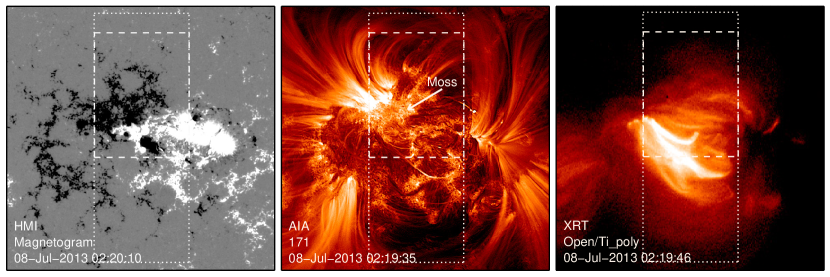
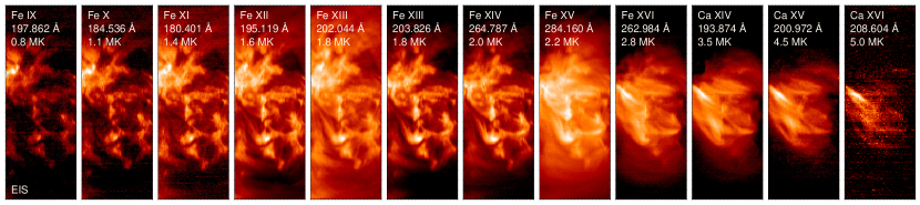
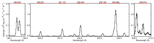
Figure 1: Observations of NOAA active region 11785 on 8 July 2013 near 2 UT. The top panels show the photospheric magnetic field measured with HMI, million degree emission observed with the AIA Fe IX 171 Å channel, and high temperature loops observed with XRT. The middle panels show EIS rasters in a series of emission lines that range in temperature of formation from 0.8 MK to 5.0 MK. The bottom panel shows an EIS spectrum near 202 Å from a single spatial pixel with the Fe XIII lines of interest highlighted. The EIS rasters are from an observation that began at 01:55 UT, and this field of view is indicated by the dotted lines in the top panels. The EIS full CCD spectrum is from an observation that began at 00:20 UT; this field of view is indicated by the dashed lines in the top panels.

The problem of interpreting astrophysical spectra is a complex one and it is tempting to account for any systematic uncertainties in the analysis with broad, ad hoc assumptions. One might assume, for example, an inflated uncertainty for each observed line intensity with the hope of encompassing the uncertainty associated with counting statistics, the radiometric calibration, and the atomic data. Such broad assumptions, however, do not account for obvious correlations within the analysis. For example, the uncertainty in the calibration clearly should be much smaller for two emission lines that are close in wavelength than for two lines that are far apart in wavelength. Similarly, the atomic data for strong lines that are the result of transitions from the ground state are likely to be more accurate than the atomic data for weak lines that are influenced by many different transitions (e.g., Foster et al., 2010).

Fortunately, recent reductions in the cost of computing have made it possible to carry out detailed statistical analysis on complex systems. Lee et al. (2011), for example, have developed a Bayesian approach for sampling from a distribution of plausible calibration curves and incorporating this information into a comprehensive analysis of high-energy Chandra spectra. Along the same theme, here we consider the effect of uncertainties in the atomic data and the problem of propagating them to the determination of plasma parameters. Since the atomic calculations involve many thousands of parameters, we cannot sample the posterior in the usual way. Thus, we develop a method that relies on a relatively small number of realizations of the atomic data to compute posterior distributions for the parameters of interest. While there still exist several computational bottlenecks in the process, we present for the first time a framework that can be applied in general to this class of problems. To begin with, we deploy a simple, but realistic, model to describe the uncertainties in some of the atomic parameters for Fe XIII, use it to generate different realizations of the plasma emissivities, then apply this ensemble of atomic data to analyze the density-sensitive Fe XIII lines observed in solar active region spectra using a Bayesian framework.

We are focusing here on Fe XIII for various reasons: it is one of the most widely used ions; several atomic calculations are available; the main lines, from the 3s² 3p 3d configuration, are well identified and strong in active regions; are mostly free of blends; and fall in a spectral region where they are observed by the EUV Imaging Spectrometer on Hinode (EIS, Culhane et al. 2007) and the radiometric calibration is relatively well understood. EIS is routinely used to measure electron densities from coronal iron ions (e.g., see Watanabe et al. 2009; Young et al. 2009). Furthermore, considering lines from a single ion removes the uncertainties related to the ionization fractions and elemental abundance, greatly simplifying the problem. Future work will expand this analysis to the calculation of the undertainties associated with emission measure distributions, which generally use observations of emission lines from different ionization stages and elements.

This paper is structured in the following way. In Section 2 we describe the Fe XIII emission lines of interest and present the traditional analysis of some representative observations. In Section 3 we develop the models for the uncertainties in the atomic data and describe how they are used to generate different realizations of the plasma emissivities. In Section 4 we present the analysis of a simple test case where we specify the plasma properties. In Section 5 we describe the application to actual observations. In Section 6 we conclude with a summary and a discussion of future work.

2 Modeling EIS Fe XIII Observations

To motivate our thinking about the data analysis, we consider the problem of determining the electron density in loop footpoints using observations of density-sensitive Fe XIII emission lines. The uncertainties in the atomic data and the analysis presented in the next sections are independent of the specific problem to which they are applied. This analysis could, for example, also be applied to measuring densities in million degree loops or measuring densities in the diffuse corona above the limb. We feel, however, that considering a specific application makes the analysis both realistic and tractable.

Figure 1 illustrates a typical observation of a solar active region. The intense magnetic fields in the active region lead to the formation of 3–4 MK plasma on the relatively short loops in the active region core (e.g., Del Zanna, 2013; Del Zanna & Mason, 2014; Warren et al., 2012). The footpoints of these high temperature loops are bright in million degree emission lines, and the footpoints are often referred to as the “moss” because of their mottled appearance in high resolution images (e.g., Berger et al., 1999; Fletcher & De Pontieu, 1999). These footpoint measurements provide information on the boundary conditions in these loops and are important for constraining models of coronal heating (e.g., Peres et al., 1994; Martens et al., 2000; Winebarger et al., 2008). Measurements of the electron density in the moss are of particular utility because they yield information on both the base pressure of the loop as well as the filling factor (Warren et al., 2008).

To further illustrate the concept of the moss, in Figure 2 we show Fe XIII 202.044 Å intensities computed from a simple, one-dimensional hydrodynamic loop model (Schrijver & van Ballegooijen, 2005). Here a relatively large volumetric heating is assumed and a loop with an apex temperature of about 3 MK is produced. As expected, the Fe XIII emission comes from a relatively localized region near the footpoint of the loop. Thus moss observations can yield information on individual loops. The emission at higher temperatures, in contrast, is generally an integration across many different loops along the line of sight, making the interpretation of such observations much more difficult.

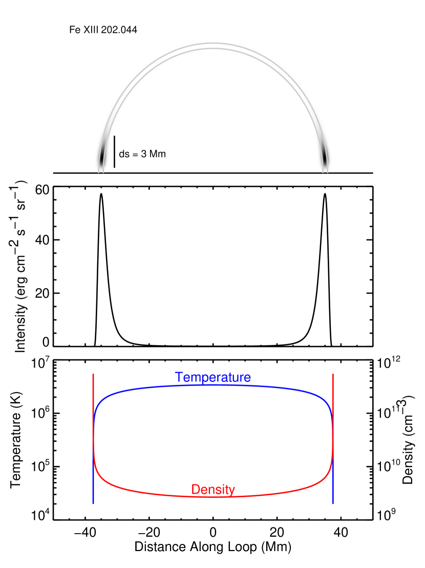
Figure 2: Density measurements in the moss can be used in conjunction with hydrodynamic loop models to infer the properties of high-temperature active region loops. The bottom panel shows the temperature and density as a function of position derived from assuming steady, uniform heating. The middle panel shows the intensity of Fe XIII 202.044 Å as a function of position along the loop. The top panel shows a rendering of the loop as it would appear viewed from the side. See Warren et al. (2008) for additional details.

Table 1: Selected Fe XIII lines observed by Hinode EIS

$i$–$j$	Identification		$\lambda_{\rm exp}$ (Å)	Notes
1–20	3s2 3p2 3P0 –	3s2 3p 3d 3P1	202.044
2–23	3s2 3p2 3P1 –	3s2 3p 3d 3D1	201.126
3–20	3s2 3p2 3P2 –	3s2 3p 3d 3P1	(209.916)	branching ratio
3–25	3s2 3p2 3P2 –	3s2 3p 3d 3D3	203.826	self-blend
3–24	3s2 3p2 3P2 –	3s2 3p 3d 3D2	203.795	self-blend
7–60	3s 3p3 3D1 –	3s 3p2 3d 3F2	203.772	self-blend
8–60	3s 3p3 3D2 –	3s 3p2 3d 3F2	203.835	self-blend
3–23	3s2 3p2 3P2 –	3s2 3p 3d 3D1	(204.942)	branching ratio
1–23	3s2 3p2 3P0 –	3s2 3p 3d 3D1	(197.431)	branching ratio
2–24	3s2 3p2 3P1 –	3s2 3p 3d 3D2	200.021
2–19	3s2 3p2 3P1 –	3s2 3p 3d 3P2	209.619
2–22	3s2 3p2 3P1 –	3s2 3p 3d 3P0	203.165	blended
4–26	3s2 3p2 1D2 –	3s2 3p 3d 1F3	196.525
2–21	3s2 3p2 3P1 –	3s2 3p 3d 1D2	(204.262)	blended

As mentioned previously, the EIS instrument on Hinode observes many emission lines whose intensities can be combined to form density-sensitive ratios. Figure 1 also shows the spectral region observed with EIS near 202 Å, which is dominated by intense Fe XIII lines. A typical analysis of these lines involves fitting each of the spectral features with Gaussians to derive the line intensities and their corresponding statistical errors. For this work we consider the lines at 196.525, 200.021, 201.121, 202.044, 203.165, 203.826, and 209.916 Å (see Table 1) and fit them with single or multiple Gaussians, as appropriate. These lines will be discussed extensively in Section 3. We have randomly selected 1000 pixels from the EIS observations of the moss shown in Figure 1 for analysis. Note that the lines at 202.044 and 209.916 Å originate in the same upper level and they form a branching ratio that is independent of solar conditions. The other five lines form density-sensitive ratios with the 202.044 Å line.

Since it is not obvious how to reconcile all of the individual line ratios, we use a simple empirical model to interpret the observations. We make the standard assumption that the intensity of an emission line can be computed with

$$I_{n}=\epsilon_{n}(n_{e},T_{e})n_{e}^{2}\,ds,$$ (1)

where $\epsilon_{n}(n_{e},T_{e})$ is the plasma emissivity, $n_{e}$ and $T_{e}$ are the electron density and temperature, and $ds$ is the effective path length through the solar atmosphere (see, for example, Mariska 1992). First, we note that since the excitation energies of the levels associated with these wavelengths are very similar, the emissivity ratios used to evaluate the plasma densities are highly insensitive to changes in temperature. Furthermore, as illustrated in Figure 2, most of the Fe XIII emission in high-temperature loops are thought to originate in a narrow region near the footpoint over which the temperatures are close to the peak temperature of formation of the ion, $\approx{1.8}$ MK. We therefore adopt this value of the temperature and henceforth treat the plasma as isothermal. Of course, hydrodynamic models show that there are gradients in temperature and density along the loop, where segments of high $n_{e}$ occupy small $ds$, and segments of small $n_{e}$ cover a large $ds$, so Equation 1 must be treated as an empirical description characterized by a representative density and effective path length.

With this empirical description, however, we can derive information about the solar atmosphere directly from the observations. The physical model shown in Figure 2 depends on additional assumptions about the loop geometry, the plasma composition, and the nature of the heating.

Table 2: Modeling Fe XIII Line Intensities in the Moss

Line	$I_{obs}$	$\sigma_{I}$	$I_{model}$	$|\Delta I|/I$(%)
196.525	1473.1 $\pm$	18.8	1443.6	2.0
200.021	1521.4 $\pm$	29.1	1749.9	15.0
201.121	2373.2 $\pm$	44.4	1987.0	16.3
202.044	2866.5 $\pm$	53.6	2989.1	4.3
203.165	775.2 $\pm$	42.5	767.5	1.0
203.826	9237.6 $\pm$	142.6	8751.2	5.3
209.916	530.2 $\pm$	56.4	516.2	2.6

For this empirical model we can use the observed intensities and their corresponding statistical uncertainties, the computed plasma emissivities, and assumed temperature to infer the best-fit electron density and path length by performing a least-squares fit. The plasma emissivites for each line is computed using version 8 of the CHIANTI atomic data base (Del Zanna et al., 2015; Dere et al., 1997).

The results of an example calculation are shown in Table 2, where we have taken the observed intensities from a single spectral pixel (arbitrarily chosen as #217) from an EIS full-CCD observation (EIS file eis_l0_20130708_002042) and applied Equation 1. The resulting best-fit parameters are $\log n_{e}=9.68\pm 0.01$ (cm^-3) and $\log ds=8.67\pm 0.02$ (cm). The error bars associated with the parameters are very small, suggesting that the parameters are very precisely determined. The uncertainties associated with the intensities, however, are also small and the standard method of determining the best-fit $n_{e}$ and $ds$ by minimizing $\chi^{2}$ results in reduced $\chi^{2}$$\approx$$30$ for this case, indicating that the model is a poor fit to the data.

This example highlights the difficulty in interpreting many solar observations. Since the sun is relatively close, we can obtain observations with high signal-to-noise. This bounty of photons, however, means that models generally do not pass rigorous statistical tests. This can be simply ignored or covered up by inflating the statistical errors with ad hoc assumptions. The real deficiency in the analysis is taking the atomic data as fixed and without uncertainty. In reality, the uncertainties associated with the plasma emissivities are likely to be comparable to or larger than those from counting statistics, and a proper data analysis must include a treatment of them. We now turn to estimating the uncertainties in the atomic data available for Fe XIII.

3 Uncertainties in the Atomic Data

The most recent (and largest) scattering calculation for Fe XIII is an $R$-matrix calculation carried out within the UK APAP network, which had a target of 749 levels up to $n=4$ (Del Zanna & Storey, 2012). The main focus of this calculation was to provide accurate data for the $n=4\to n=3$ soft X-ray transitions. Indeed, new lines in this wavelength range were subsequently identified (Del Zanna, 2012a). The scattering calculation was supplemented by a structure calculation which was used to calculate the radiative data, using either observed or empirically-adjusted theoretical wavelengths. The scattering and radiative data produced in this calculation were recently made available within the CHIANTI database in its version 8 (Del Zanna et al., 2015). We use these data as our baseline.

Storey & Zeippen (2010) previously carried out a similar scattering calculation (using the same $R$-matrix method and the same codes), the only difference being that it was aimed at improving the earlier calculations for the $n=3$ levels. The target had a total of 114 fine-structure levels, and included only some $n=4$ levels.

Del Zanna & Storey (2012) also performed separate calculations for the $n=5,6$ levels, but showed that cascading effects are small when considering the strong EUV lines emitted by the $n=3$ levels. The same paper also showed that the intensities of the transitions from the $n=3$ levels are close to those of the previous Storey & Zeippen (2010) model.

The Storey & Zeippen (2010) atomic data provided very good agreement between observed and theoretical intensities of the strongest EUV lines, as shown in one of the benchmark works by Del Zanna (2011), based on a variety of sources, including Hinode/EIS. Del Zanna (2011) also benchmarked other atomic data for this ion, calculated by Gupta & Tayal (1998) and Aggarwal & Keenan (2005). Various shortcomings in these calculations were found. On the other hand, excellent agreement (to within a relative 10%) was found for the main lines observed by Hinode EIS in an active region moss area and the Storey & Zeippen (2010) atomic data, already indicating an excellent accuracy in both the experimental and theoretical data, as we will also confirm below.

The Del Zanna (2011) benchmark work also reviewed all the previous identifications and determined which lines are likely to be blended, and hence avoided in our analysis. The main lines chosen for our study are listed in Table 1, in order of decreasing intensity. The main line is the straight decay to the ground state, which produces the emission line at 202.044 Å. We note that two transitions from the 3s 3p² 3d ³F₂ were suggested to be blending the main density diagnostic line, already a self-blend at 203.8 Å. However, as noted by Del Zanna (2011), at the high densities that are considered here these lines do not have a significant contribution, so even if the identifications were incorrect the results presented here would still stand. The other lines (at 201.126, 200.021, 209.619, 203.165 Å) have a similar density sensitivity as the 203.8 Å one, except the 196.525 Å, which decays to a more excited level. The 203.165 Å was shown to be blended at low densities. Some lines (with wavelengths in brackets) were not considered since they are branching ratios (decays from the same upper level) with other lines we have included. Further benchmarks were carried out by Del Zanna (2012b).

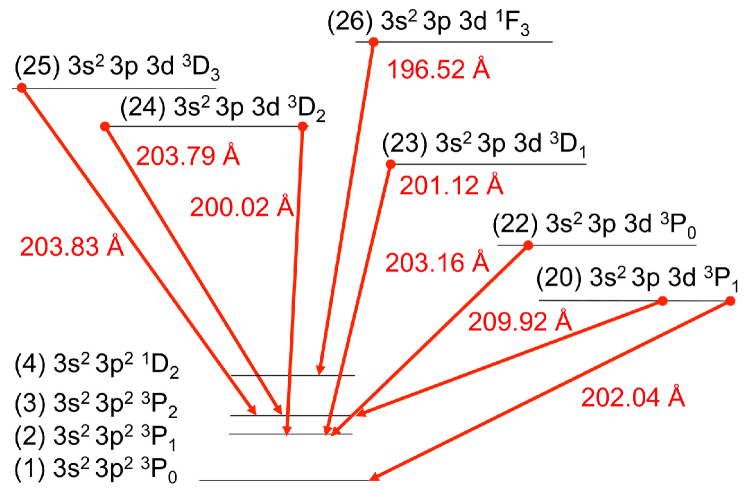
Figure 3: A simplified level diagram for the transitions relevant to the lines considered in this paper.

Figure 4: Percentage difference in the thermally-averaged collision strengths (Storey & Zeippen (2010) vs. Del Zanna & Storey (2012)), for a selection of transitions (top: to the 3s² 3p 3d levels; bottom: to the other $n=3$ levels). The dashed lines represent the approximate uncertainties used to generate alternative realizations of the atomic data for Fe XIII.

The intensity of a spectral line is proportional to the population of the upper level and the spontaneous transition probability (the A-value). To assess which atomic rates affect a spectral line, it is therefore important to check which are the main populating mechanisms for each level. A simplified level diagram for the main transitions discussed in this section is provided in Figure 3, for a specific density. However, the main populating mechanisms for each atomic level normally vary with the density, so the issue can become quite complex to describe. Some details will be discussed in a separate paper, where also the various parameters that can affect an atomic calculation are reviewed. In summary, the 202.044 Å line is mainly populated by direct excitation from the 3s² 3p^{2 3}P₀ ground state via a strong dipole-allowed transition. The various calculations provide the same rate, within a few percent. In turn, the population of the ground state decreases significantly as the population of the metastable levels increases. On the other hand, the populations of the other levels which produce the other lines in Table 1 are mainly driven by excitations from all the 3s² 3p^{2 3}P_0,1,2 levels, although non-negligible contributions (typically 10–30%) come also from cascading from higher levels.

Figure 5: Scatter plot of the thermally-averaged collision strengths calculated by Del Zanna & Storey (2012) with the $R$-matrix codes (as in CHIANTI, present), vs. with the DW approximation. Dash and dot-dash lines indicate a $\pm$ 20, 50%.

It is therefore important to first assess how accurate the rates of excitation from the 3s² 3p^{2 3}P_0,1,2 to the 3s² 3p 3d levels are. We have chosen to compare the latest values with those calculated by Storey & Zeippen (2010), because the two calculations were very similar, i.e. the main differences are caused by the size of the target and not by the method of the calculation. As already shown by Del Zanna & Storey (2012), the largest calculation provides very similar rates for the stronger lines, but significantly increased values for the weaker ones, as one would expect. We have considered only excitations from the 3s² 3p^{2 3}P_J and 3s² 3p^{2 1}D₂ levels (the only ones with significant population) at the temperature of peak ion abundance in ionization equilibrium (2 MK, see Figure 4 top). As an estimate of the uncertainty in the strongest lines, with collision strengths above 1.0, we have taken 5%, which is well above the scatter of values. For the weaker lines, we have taken as an estimate the dashed line, i.e. a linear increase (up to a maximum of 50%).

We have then considered all the excitations to the remainder of the $n=3$ levels calculated by Storey & Zeippen (2010), taking into account the different level orderings of the two calculations. In this case, we have taken a 10% uncertainty for the transitions above 0.1, and the linear increase shown in Figure 4 (bottom, up to a maximum of 50%).

One possible estimate for all the $n=3$ levels not included in Storey & Zeippen (2010) and all the $n=4$ levels is to compare the full scattering calculation with the results of the distorted-wave (DW) calculation carried out by Del Zanna & Storey (2012), which does not include resonance enhancements (see Figure 5). We have taken a 20% uncertainty for the transitions above 0.01 and 50% for the weaker transitions.

Figure 6: Percentage difference in the A-values calculated by Young (2004) and Del Zanna & Storey (2012) within the lowest 27 levels.

The next step is to provide an estimate on the uncertainty of the A-values. As shown by Young (2004), different calculations can provide significantly different values. For our estimates, we have chosen to compare the Del Zanna & Storey (2012) A-values with those calculated by Young (2004) with the SUPERSTRUCTURE program (Eissner et al., 1974). An extended configuration set was used by Young (2004) to calculate radiative data for this ion. This data were made available within CHIANTI version 4 (Young et al., 2003) in 2003. Figure 6 shows comparisons of the A-values for all the transitions within the lowest 27 levels, which include the 3s² 3p 3d.

We have taken for transitions having an A-value above 10¹⁰ an uncertainty of 5%, for those between 10⁸ and 10¹⁰ 10%, while for weaker transitions, 30%. For the forbidden transitions within the ground configuration: we have taken 10%.

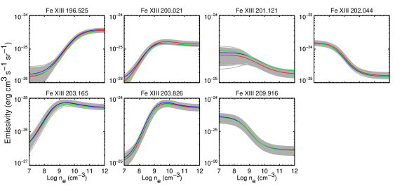
Figure 7: Emissivities of the seven Fe XIII lines considered in this work. The emissivities are computed assuming a temperature of 1.8 MK, the temperature of formation for Fe XIII. The gray lines represent the 1000 realizations of the CHIANTI atomic data. The red curve is the default value from CHIANTI v.8. As discussed in Section 5, the blue curve is identified as being most probable match to the observations (#471) and the green curve the second most probable (#368).

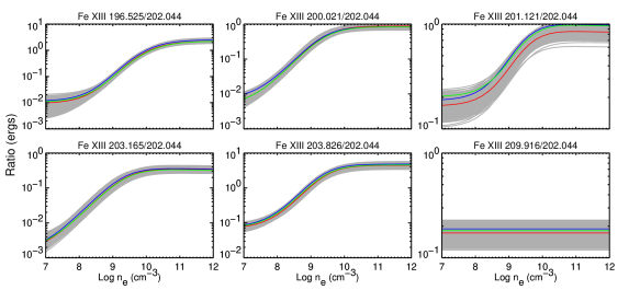
Figure 8: The theoretical ratios of six Fe XIII lines with respect to Fe XIII 202.044. See Figure 7 for additional details.

We have modified the standard CHIANTI IDL routines distributed in SolarSoft (SSW, Freeland & Handy 1998) to assign to each transition an uncertainty in the A-value and in the excitation rate. We used the IDL function randomn to randomly vary each rate within the estimated uncertainty. The distribution is normal, in the sense that if, e.g., an uncertainty is 10%, most values will vary within $\pm$ 20%. We then used the standard CHIANTI routine (emiss_calc) to calculate the line emissivities. For each of the seven chosen lines, we have added any Fe XIII lines within $\pm$ 0.1 Å to take self-blends into account. We have generated a total of 1000 realizations of the emissivities for each line, which are shown in Figure 7. The figure clearly shows how the spectral lines vary their emissivities as a function of the density. Figure 8 shows the variation of ratios with density.

By attaching reasonable uncertainties to the atomic data we can generate realizations of the emissivities that capture this uncertainty. We can then use the ensemble of emissivities to characterize parameters like plasma densities and column heights. Our methodology for combining an ensemble of emissivities with observed data to account for uncertainties in atomic data is described in detail in Section 5.

4 Simulated Datasets

The next step in this analysis is to generate sets of intensities from known densities and path lengths. This will allow us to test our ability to recover physical parameters from the Fe XIII intensities and to illustrate how the variations in the atomic data developed in the previous section lead to variations in the inferred densities and path lengths. These intensities complement the set of observed intensities taken from the data illustrated in Figure 1.

The ratio curves shown in Figure 8 indicate that these lines are sensitive to density in the range of $n_{e}$ of $10^{8}$ to $10^{11}$ cm^-3. Thus we randomly select 1000 densities uniformly on the interval $\log n_{e}=[8.5,10.5]$. To continue with our theme of analyzing observations of active region moss we use the theoretical estimate of the moss path length from Martens et al. (2000) of

$$ds=\frac{2.56\times 10^{8}}{P_{0}},$$ (2)

where $P_{0}=2k_{b}n_{e}T_{e}$ is in dyne cm^-2, $k_{b}$ is the Boltzmann constant, and $ds$ is in cm. Again, we use the peak temperature of formation for Fe XIII, 1.8 MK, for this calculation. Note that this expression was derived for somewhat cooler emission and we do not expect it to track the Fe XIII path lengths exactly.

Each set of density and path length can be used to generate a set of intensities using statistics using the EIS pre-flight effective areas and the assumption of a 60 s exposure time and the 2″ slit. Finally, we do not use these computed intensities directly when attempting to recover them with the model. We first apply a normally distributed random perturbation to each intensity, which mimics the variations in measured counts expected due to the finite exposure time.

Table 3: Modeling Fe XIII Line Intensities in the Moss

Line	$I_{obs}$	$\sigma_{I}$	$I_{model}$	$|\Delta I|/I$(%)
196.525	751.0 $\pm$	9.4	750.7	0.0
200.021	678.7 $\pm$	11.8	694.7	2.4
201.121	750.7 $\pm$	14.8	748.6	0.3
202.044	1012.5 $\pm$	20.6	1011.9	0.1
203.165	313.7 $\pm$	13.7	296.2	5.6
203.826	3533.1 $\pm$	52.2	3498.8	1.0
209.916	168.4 $\pm$	21.0	174.8	3.8

An example set of simulated intensities is given in Table 3 for assumed values of $\log n_{e}=9.90$ and $\log ds=7.80$. If we use the standard set of CHIANTI emissivities to model these intensities we recover the input parameters almost exactly, $\log n_{e}=9.90\pm 0.01$ and $\log ds=7.82\pm 0.03$. As with the example set of observed intensities in Table 2, the uncertainties on these parameters are very small. Unlike the case with the observed intensities, however, we obtain a reduced $\chi^{2}$ of order 1.

5 Inference

The standard method of $\chi^{2}$ minimization (see Section 2) allows best-fit values of the plasma density $n_{e}$ and column depth $ds$ to be determined for a given pixel, under the assumption that the emissivity curves are completely and correctly specified.

Now, equipped with $1000$ datasets corresponding to randomly selected EIS pixels, we can consider the uncertainties in the fitted density and path length in each case that result from both statistical fluctuations in the observed intensities and the atomic data uncertainties incorporated in the ensemble of CHIANTI emissivities. To do so, we develop a Bayesian methodology that first assumes the observed data is uninformative regarding the atomic physics (the so-called pragmatic Bayesian method) and then incorporate the potential information in the observed data to learn about the atomic physics (the fully Bayesian method). The fully Bayesian method is a principled statistical analysis, while the pragmatic method makes simplifying assumptions that tend to overestimate the final uncertainty on the fitted density and path length. More details of the distinction between the two methods is discussed in Section 5.4. We start by providing an introduction to Bayesian inference in Section 5.1.

5.1 Bayesian Inference

We take a Bayesian approach in our statistical analysis because it enables us to build in the complex hierarchical dependencies engendered by atomic uncertainties. Such an approach offers a probability-based formalism for combining information from our prior knowledge and the current data. This requires both a prior distribution, which quantifies the uncertainty in the values of the unknown model parameters before the data is observed, and a likelihood function — the distribution of the data given the model parameters. The likelihood function allows us to assess the viability of a parameter value given the observed data under a proposed statistical model. The likelihood function is combined with the prior distribution to yield the posterior distribution, which quantifies the uncertainty in the values of the unknown model parameters taking account of the observed data. If we let $X$ and $\psi$ represent generic data and unknown model parameters, respectively, Bayes’ theorem provides the posterior distribution as

$$p(\psi|X)=\frac{L(\psi|X)\ p(\psi)}{p(X)},$$ (3)

where $L(\psi|X)$ is the likelihood of $X$ given $\psi$ (sometimes written as $p(X|\psi)$) and $P(\psi)$ the prior distribution of $\psi$. The term $P(X)$ is a normalizing constant necessary to make $p(\psi|X)$ a proper probability distribution. (The term $p(X)$ is sometimes referred to as the ”evidence” in the astrophysics literature.) The posterior distribution, which combines information in the data with our prior knowledge, is our primary statistical tool for deriving parameter estimates and their uncertainties.

To perform a Bayesian analysis of the Fe XIII intensities, we start by defining notation and terminology in Section 5.2. We specify the likelihood function and the prior distribution in Section 5.3. In Section 5.4, we derive the posterior distribution under two sets of assumptions, which result in the aforementioned pragmatic Bayesian and fully Bayesian approaches. In Section 5.5 and Section 5.6 we discuss our model-fitting routines, separate pixel-by-pixel and simultaneous analyses, where we consider the $1000$ pixel datasets individually and simultaneously. In Section 5.7 and Section 5.8 we apply our methodologies to the simulated and the observed intensities, respectively.

5.2 Notation

Suppose that in each of $K=1000$ pixels we observe the intensities of each of $J$ spectral lines with wavelengths $\Lambda=\{\lambda_{1},\ldots,\lambda_{J}\}$. Let $I_{k\lambda}$ be the observed intensity of the line with wavelength $\lambda\in\Lambda$ in pixel $k\in\{1,\ldots,K\}$, $\sigma_{k\lambda}$ its known standard deviation, $D_{k}=(I_{k\lambda_{1}},\ldots,I_{k\lambda_{J}})$, and $\mathcal{D}=\{D_{1},\ldots,D_{K}\}$.

We also have a collection of $M=1000$ realizations of the plasma emissivities, denoted by $\mathcal{M}$,

$$\mathcal{M}=\{\epsilon_{\lambda}^{(m)}(n_{ek},T_{ek}),\lambda\in\Lambda,m=1,\ldots,M\},$$

where $n_{ek}$ and $T_{ek}$ are the electron density and temperature for pixel $k$ and $m$ indexes the emissivity realization (i.e., emissivity curve, $\epsilon_{\lambda}^{(m)}(n_{ek},T_{ek})$), with $m$=$1$ corresponding to the default CHIANTI emissivities.

The expected intensity of the line with wavelength $\lambda$ in pixel $k$ can be rewritten (from Eq (1)) as $\epsilon_{\lambda}(n_{ek},T_{ek})n_{ek}^{2}ds_{k}$, where $ds_{k}$ is the path length through the solar atmosphere for pixel $k$. Let $\theta_{k}=(\log n_{ek},\log ds_{k})$ be the plasma parameters in pixel $k$, and $\Theta=(\theta_{1},\ldots,\theta_{K})$.

5.3 Statistical Model

The first step in specifying our statistical model is to construct the likelihood function. We model the intensities $I_{k\lambda}$ given $m$, $n_{ek}$, and $ds_{k}$ as a normal (i.e. Gaussian) distribution,

$$I_{k\lambda}\mid m,n_{ek},ds_{k}\mathbin{\overset{\rm{indep}}{\kern 0.0pt\sim}}\mathcal{N}\left(\epsilon_{\lambda}^{(m)}(n_{ek},T_{ek})n_{ek}^{2}ds_{k},\,\sigma^{2}_{k\lambda}\right),$$ (4)

for $\lambda\in\Lambda$, where $\mathcal{N}(\mu,\sigma^{2})$ is a normal distribution with mean $\mu$ and variance $\sigma^{2}$. We suppress the conditioning on the $\sigma_{k\lambda}$ throughout for notational simplicity. Thus the likelihood function of $D_{k}$ given emissivity index, $m$, and plasma parameters, $\theta_{k}$, is

$$\begin{split}L(m,\theta_{k}\mid D_{k})&=p(D_{k}\mid m,\theta_{k})\\ &=\prod_{j=1}^{J}\mathcal{N}\left(\left.I_{k\lambda_{j}}\ \right|\ \epsilon_{\lambda_{j}}^{(m)}(n_{ek},T_{ek})n_{ek}^{2}ds_{k},\ \sigma^{2}_{k\lambda_{j}}\right),\end{split}$$ (5)

where $\mathcal{N}(x\mid\mu,\sigma^{2})$ is the density of a normal distribution with mean $\mu$ and variance $\sigma^{2}$ evaluated at $x$. Note that we focus on methods that treat the emissivity index $m$ as an unknown parameter, whose prior is specified below, whose posterior we estimate to determine the most likely emissivity realizations among those in $\mathcal{M}$, and whose uncertainties affect both the fit and error bars of $\theta_{k}$.

Next, we specify the joint prior distribution on the unknown model parameters. For $\log n_{ek}$ and $m$ we specify a continuous uniform distribution and a discrete uniform distribution, respectively,

$$p(\log n_{ek}) =\frac{1}{5}\quad\ \ \text{for }7\leq\log n_{ek}\leq 12,$$ (6)

$$p(m) =\frac{1}{M}\quad\text{for each }m=1,\ldots,M.$$ (7)

This choice of prior on $m$ stipulates that the $1000$ realizations of emissivity curves in $\mathcal{M}$ are all a priori equally likely to be the true emissivity. As the realizations were generated by attaching reasonable uncertainties to the atomic data as described in Section 3, the atomic data uncertainties are contained in $p(m)$ and are thus captured by the corresponding posterior distribution. Therefore, the $1000$ realizations of emissivity curves can also be considered as a sample of $1000$ draws from an implicit prior distribution.

For $\log ds_{k}$, however, a uniform prior, $p(\log ds_{k})\propto 1$, yields an improper posterior distribution because the likelihood converges to a positive constant as $\log ds_{k}$ goes to $-\infty$. Therefore, we specify a Cauchy distribution for $p(\log ds_{k})$,

$$\log ds_{k}\sim\text{Cauchy}(\text{center}=9,\ \text{scale}=5).$$ (8)

which is a broad, fat-tailed distribution covering all conceivable values for the path length that we expect based on all sets of Fe XIII intensities, with an example set of intensities shown in Table 2.

We assume the parameters are independent a priori so that the joint prior distribution is

$$\begin{split}p(m,\theta_{k})&=p(m)\ p(\theta_{k})\\ &=p(m)\ p(\log n_{ek})\ p(\log ds_{k}).\end{split}$$ (9)

Here $\theta$ is indexed by $k$, but $m$ is not. This reflects the fact that, although $\theta_{k}$ vary among the pixels, we expect the true emissivity (i.e., the true value of $m$) to be an underlying physical quantity that is the same for all pixels.

We consider two ways to fit the plasma parameters, $\Theta$, given the observed or simulated intensities, $\mathcal{D}$, while accounting for atomic uncertainty, $\mathcal{M}$. First we can analyze each pixel separately in a sequence of pixel-by-pixel analyses. Although this may yield different estimates of $m$, the index of the preferred emissivity curve among the pixels, it allows us to see if the intensities of each pixel give consistent information as to the best emissivity curve(s). Alternatively, we can simultaneously analyze the intensities from all the pixels to arrive at an overall estimate of the most likely emissivity curve. Using this strategy, uncertainty can be quantified with a list of the most likely emissivity realizations from $\mathcal{M}$ (or their indices, $m$) along with their associated posterior probabilities.

We consider both the separate pixel-by-pixel and simultaneous analyses, and for each develop both pragmatic and fully Bayesian approaches. Specifically, Section 5.4 develops the pragmatic and fully Bayesian approaches to the pixel-by-pixel analyses and Section 5.5 describes the algorithms used to deploy these approaches. The simultaneous analysis and its algorithm are discussed in Section 5.6.

5.4 Pragmatic and fully Bayesian methods for separate pixel-by-pixel analysis

Given the likelihood function in Eq (5) and the prior distribution in Eq (9), the joint posterior distribution for $m$ and $\theta_{k}$ under the separate pixel-by-pixel analyses is

$$p(m,\theta_{k}|D_{k})=\frac{L(m,\theta_{k}\mid D_{k})\ p(m,\theta_{k})}{p(D_{k})},$$ (10)

where $p(D_{k})=\sum_{m=1}^{M}\int L(m,\theta_{k}\mid D_{k})\ p(m,\theta_{k})\ \mathrm{d}\theta_{k}$.

Then the marginal posterior distribution $p(\theta_{k}\mid D_{k})$ can be obtained by summing over $m$,

$$p(\theta_{k}\mid D_{k})=\sum_{m=1}^{M}p(m,\theta_{k}\mid D_{k}).$$ (11)

In this way, we are able to infer $\theta_{k}$ accounting for uncertainties of the atomic data via the ensemble in $\mathcal{M}$.

5.4.1 Pragmatic Bayesian method

For the pragmatic Bayesian method, as described by Lee et al. (2011), we assume that the observed intensities are uninformative as to the most likely emissivities. That is, we do not take into account the information in the intensities for narrowing the uncertainty in the choice of emissivity realizations. Mathematically, this assumption can be written $p(m\mid D_{k})=p(m)$, i.e., $m$ and $D_{k}$ are independent. Thus, the pragmatic Bayesian joint posterior distribution of $m$ and $\theta_{k}$ is

$$p(m,\theta_{k}\mid D_{k}) =p(\theta_{k}\mid D_{k},m)\ p(m\mid D_{k})$$ (12)

$$=p(\theta_{k}\mid D_{k},m)\ p(m),$$ (13)

and the marginal posterior distribution of $\theta_{k}$ (from Eq (11)) is

$$\begin{split}p(\theta_{k}\mid D_{k})&=\sum_{m=1}^{M}p(m,\theta_{k}\mid D_{k})\\ &=\sum_{m=1}^{M}p(\theta_{k}\mid D_{k},m)\ p(m).\end{split}$$ (14)

The pragmatic Bayesian method accounts for atomic uncertainty in a conservative manner. The assumption that $p(m\mid D_{k})=p(m)$ ignores information in the intensities, $D_{k}$, that may reduce uncertainty of atomic data represented by $m$ and hence of $\theta_{k}$. We now consider methods that allow $D_{k}$ to be informative for $m$.

5.4.2 Fully Bayesian method

In contrast to the pragmatic Bayesian method, the fully Bayesian method, as described by Xu et al. (2014), incorporates the potential information in the data (i.e., the intensities) to learn about $m$. The fully Bayesian joint posterior distribution of $m$ and $\theta_{k}$ is given in Eq (12) and the marginal posterior distribution of $\theta_{k}$ is given by

$$\begin{split}p(\theta_{k}\mid D_{k})&=\sum_{m=1}^{M}p(m,\theta_{k}\mid D_{k})\\ &=\sum_{m=1}^{M}p(\theta_{k}\mid D_{k},m)\ p(m\mid D_{k})\end{split}$$ (15)

where each $p(\theta_{k}\mid D_{k})$ is normalized so that $\sum_{m=1}^{M}p(m\mid D_{k})=1$.

Using Bayes’ theorem, we can directly compute the probability of each emissivity realization, $m$, given the data in each pixel separately,

$$p(m\mid D_{k})=\frac{p(D_{k}\mid m)}{\sum_{m=1}^{M}p(D_{k}\mid m)}.$$ (16)

This is the marginal posterior probability among those emissivity realizations in $\mathcal{M}$. Eq (16) holds because each of the $m$ has the same prior probability (see Eq (7)).

The Bayesian posterior distribution in Eq (16) allows the observed intensities to be informative for the atomic physics, following the principles of Bayesian analysis (Xu et al., 2014). It enables us to use the intensities to determine which emissivity realizations are more or less likely and averages over (posterior) uncertainty in emissivity realizations.

5.5 Algorithms for the separate pixel-by-pixel analyses

5.5.1 Algorithms for pragmatic Bayesian in the separate pixel-by-pixel analyses

The Metropolis-Hastings (MH) algorithm (e.g., Hastings, 1970) is a general term for a family of Markov chain simulation methods that are useful for sampling from Bayesian posterior distributions. Let $p(\psi|X)$ be the target posterior distribution, using the notations in Section 5.1. A proposed $\psi^{*}$ is sampled from a proposal distribution $q(\psi^{*}|\psi^{(t)})$ at iteration $t+1$. Calculating the acceptance probability, $\rho=\frac{p(\psi^{*}|X)\ q(\psi^{(t)}|\psi^{*})}{p(\psi^{(t)}|X)\ q(\psi^{*}|\psi^{(t)})}$, we set $\psi^{(t+1)}=\psi^{*}$ with probability $\min(\rho,1)$ and set $\psi^{(t+1)}=\psi^{(t)}$ otherwise.

To obtain a Monte Carlo (MC) sample of $(m,\theta_{k})$ from the pragmatic Bayesian posterior in Eq (13), we first obtain a MC sample of the emissivity index, $\{m^{(1)},\ldots,m^{(L)}\}$, from its prior distribution, Eq (7). For each $m^{(\ell)}$, with $\ell=1,\dots,L$, we can then sample $\{\theta_{k}^{[\ell,t]},t=1,\ldots,T\}$ from $p(\theta_{k}\mid m^{(\ell)},D_{k})$ using the MH algorithm. This requires that we specify the proposal distribution $q(\theta^{*}|\theta^{(t)})$. To do so, we first compute the value of $\theta_{k}$ that maximizes $\log p(\theta_{k}\mid m^{(\ell)},D_{k})$, i.e., the maximum a posteriori (MAP) estimates, $\hat{\theta}_{k}$, along with the $2\times 2$ Hessian matrix evaluated at the mode $\hat{\theta}_{k}$, $H(\hat{\theta}_{k})$, for each $m^{(\ell)}$. We then use $t_{4}\left(\theta_{k}\mid\hat{\theta}_{k},(-H(\hat{\theta}_{k}))^{-1}\right)$ as the MH proposal distribution, where $t_{\nu}\left(x\mid\mu,\Sigma\right)$ is the density of a multivariate $t$ distribution with $\nu$ degrees of freedom, mode $\mu$, and scale matrix $\Sigma$, evaluated at $x$. This type of MH sampler is known as an independence sampler (Gilks et al. 1996). We run MH for $T$ iterations, the last of which is taken as the MC sample corresponding to $m^{(\ell)}$, i.e., $\theta_{k}^{(\ell)}=\theta_{k}^{[\ell,T]}$.

5.5.2 Algorithms for fully Bayesian in the separate pixel-by-pixel analyses

In the fully Bayesian separate pixel-by-pixel analyses, our aim is to obtain a MC sample from the joint posterior distribution, Eq (12), and we propose three basic strategies for doing this: (i) two-step MC with MH, described in Section 5.5.3 and Appendix A, (ii) two-step MC with a Gaussian approximation, described in Appendix B, and (iii) Hamiltonian MC (HMC), described in Appendix C. Specifically, the first strategy uses the MH algorithm while the second strategy makes a Gaussian approximation to the conditional distribution of $\theta_{k}$ given the sampled emissivity realization $m$, respectively. Comparing the three strategies, the two-step MC with MH is preferred because of the accuracy of estimates with moderate computation time, while two-step MC with a Gaussian approximation may be faster (but less accurate) and HMC can be more accurate (but slower) under certain conditions.

5.5.3 Implementation of two-step MC with MH for fully Bayesian in the separate pixel-by-pixel analyses

In order to implement the fully Bayesian method and to obtain a MC sample of $\theta_{k}$ via Eq (15), we first evaluate Eq (16) for each $m$ where

$$p(D_{k}\mid m)=\int L(m,\theta_{k}\mid D_{k})\,p(\theta_{k})\,\mathrm{d}\theta_{k}$$ (17)

is the Bayesian evidence conditional on a given emissivity. For each sampled $\theta_{k}$, we need only evaluate the likelihood for $m=1,\ldots,M$, and then renormalize the $M$ likelihood values by this weighted sum, which can be achieved via a two-step sampling as described in this section.

The two dimensional integral in Eq (17) can be evaluated numerically using the grid generated from the Trapezoidal Quadrature Rule (TQR), which is suitable for finite domain quadrature . The Product-Rule is also used in the construction of multivariate grids, which leads to an evenly designed grid.

The two dimensional quadrature can then be expressed as

$$\int L(m,\theta_{k}\mid D_{k})\,p(\theta_{k})\,\mathrm{d}\theta_{k}\\ =\sum_{i,j}w_{i,j}\,L(m,\log n_{ek}^{(i)},\log ds_{k}^{(j)}\mid D_{k})\,p(\log n_{ek}^{(i)},\log ds_{k}^{(j)})$$ (18)

where nodes $(\log n_{ek}^{(i)},\log ds_{k}^{(j)})$ and weights $(w_{i,j})$ are defined by the chosen quadrature rule . The integral range of the two parameters is $(\hat{\theta}_{k}-3\times\text{sdev}_{k},\hat{\theta}_{k}+3\times\text{sdev}_{k})$ where $\text{sdev}_{k}$ is a vector of the square root of the diagonal elements in variance-covariance matrix $(-H(\hat{\theta}_{k}))^{-1}$.

Having evaluated Eq (16) at each $m$, we can obtain a MC sample of the emissivity index, $\{m^{(1)},\ldots,m^{(L)}\}$. For each $m^{(\ell)}$ we sample from $p(\theta_{k}\mid D_{k},m^{(\ell)})$ using an independence sampler exactly as described in Section 5.5.1. For each $m^{(\ell)}$, we run the independence sampler for $T$ iterations to obtain the MC sample corresponding to $m^{(\ell)}$, $\theta_{k}^{(\ell)}=\theta_{k}^{[\ell,T]}$. The detailed two-step MC with MH ($\mathcal{S}_{MH}$) is given in Appendix A.

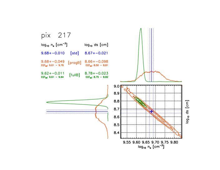
Figure 9: Comparisons of the inferred density $n_{e}$ and path length $ds$ using different methods for pixel #$217$ (for the intensities listed in Table 2). The results from the different methods used are color coded, with blue representing the standard method, red the pragmatic Bayes method (Section 5.4.1), and green the fully Bayes method (Section 5.4.2) with the latter two computed for all pixels simultaneously (see Section 5.6). The contour plots (with levels at $0.01\times$, $0.1\times$, and $0.5\times$ the maximum) show where the majority of the mass of the joint probability distributions of $(n_{e},ds)$ fall, and their marginalized distributions along each axis is shown to the top and to the right of the corresponding axis. The results from the standard analysis is shown along with the histograms as straight lines (solid for the best-fit and dashed denoting the $\pm 1\sigma$ errors on the best-fit obtained from the default CHIANTI emissivity functions), extending into the contour plot region. The best-fit value from standard analysis is also marked on the contour plot with a ’+’ sign, with the arms of the symbol corresponding to the sizes of the error bars. The standard deviations of the marginalized posterior densities, as well as the $90$% equal-tail bounds for both the pragmatic and full Bayes cases are listed in the legend. As expected, the density and path length are highly correlated. The standard method underestimates the uncertainties, the pragmatic Bayes method inflates them due to atomic data uncertainties. The fully Bayes method strikes a balance between atomic data uncertainties and how well the data are fit, shrinking the error bars relative to pragmatic Bayes and shifting the estimates. The full set of plots for all $1000$ pixels considered here are available as a supplementary figure in the online journal.

5.6 Simultaneous analysis

When we consider all the $K$-pixel intensities together in a simultaneous analysis using the fully Bayesian method, the likelihood function of $m$ and $\Theta$ given $\mathcal{D}$, and the prior distribution of $m$ and $\Theta$ are, respectively,

$$L(m,\Theta\mid\mathcal{D})=\prod_{k=1}^{K}L(m,\theta_{k}\mid D_{k})$$ (19)

and

$$p(m,\Theta)=p(m)\ \prod_{k=1}^{K}p(\theta_{k}).$$ (20)

Thus, the joint posterior distribution of $m$ and $\Theta$ can be expressed as

$$p(m,\Theta\mid\mathcal{D})=\frac{L(m,\Theta\mid\mathcal{D})p(m,\Theta)}{p(\mathcal{D})},$$ (21)

where $p(\mathcal{D})=\sum_{m=1}^{M}\int L(m,\Theta\mid\mathcal{D})p(m,\Theta)\ \mathrm{d}\Theta$. Similarly, treating $m$ as an unknown parameter, we express the left hand side of Eq (21) as

$$p(m,\Theta\mid\mathcal{D})=p(\Theta\mid\mathcal{D},m)\ p(m\mid\mathcal{D}),$$ (22)

and we conduct statistical inference by obtaining a MC sample from this joint posterior distribution.

First we can use all the data simultaneously to obtain the marginal posterior probability of each emissivity realization $m$,

$$p(m\mid\mathcal{D})=\frac{\prod_{k=1}^{K}p(D_{k}\mid m)}{\sum_{m=1}^{M}\prod_{k=1}^{K}p(D_{k}\mid m)}.$$ (23)

and sample $m^{(\ell)}$, for $\ell=1,\ldots,L$, with weights given by the marginal posterior probabilities in Eq (23) so that those favoured by the data are sampled more frequently. The computation of $p(D_{k}\mid m)$ for each $k$ and $m$ is discussed in Section 5.5.3.

For each sampled $m$, we sample $\theta$ from its conditional posterior distribution

$$\begin{split}p(\Theta\mid\mathcal{D},m)&\propto L(m,\Theta\mid\mathcal{D})\ p(\Theta)\\ &=\prod_{k=1}^{K}L(m,\theta_{k}\mid D_{k})\ p(\theta_{k})\\ &=\prod_{k=1}^{K}\prod_{j=1}^{J}\mathcal{N}\left(\left.I_{k\lambda_{j}}\ \right|\ \epsilon_{\lambda}^{(m)}(n_{ek},T_{ek})n_{ek}^{2}ds_{k},\ \sigma^{2}_{k\lambda_{j}}\right)\\ &\times p(\log n_{ek})\ p(\log ds_{k}).\end{split}$$ (24)

as these $K$-pixel datasets were randomly selected from the observations indicated in Section 2, so that we can safely assume conditional independence among them.

Similarly, an MH sampler is used to obtain a correlated MC sample, $\{\Theta^{[t]},t=1,\ldots,T\}$, from $p(\Theta\mid m^{(\ell)},\mathcal{D})$. A $t_{4}\left(\theta_{k}\mid\hat{\theta}_{k},(-H(\hat{\theta}_{k}))^{-1}\right)$ proposal distribution is used for each pixel independently and separately to make the computation more efficient. With this proposal distribution, we run the MH for $T$ iterations over all the $K$-pixel intensities and obtain the MC sampler corresponding to $m^{(\ell)}$, $\Theta^{(\ell)}=\Theta^{[\ell,T]}$. The detailed two-step MC with MH via simultaneous analysis ($\mathcal{S}_{MH_{simul}}$) is given in Appendix D.

5.7 Application to simulated intensities

Here we illustrate both the separate pixel-by-pixel and the simultaneous analyses, mentioned in Section 5.5 and Section 5.6, with a simulated case, using $K=1000$ simulated sets of intensities for each of $J=7$ spectral lines with known density and path lengths as described in Section 4. This will allow for the comparison of our inferred values with known values.

We run the separate pixel-by-pixel and simultaneous analyses described in Section 5.5.3 and Section 5.6. For both analyses, $30$ MH samplers, which is determined by constructing autocorrelation plots in this setting (Xu et al., 2014), are drawn for each sampled emissivity realization $m^{(\ell)}$, and the last MH sampler is taken as a MC sampler. There are $8000$ MC samplers drawn in each simulation.

The comparison of the relative posterior probability $p(m\mid D_{k})$ for each emissivity index and for each pixel, in separate pixel-by-pixel analyses, is shown in the left panel of Figure 10. The emissivity realization with index $1$ occupies almost all of the probability. Similarly, in the simultaneous analysis, the posterior probability of the emissivity realization with index $1$ is nearly to one. Both analyses recover the fact that all of the simulated sets of intensities are computed from the actual CHIANTI atomic data (the emissivity realization with index $1$) instead of the perturbed atomic data as described in Section 4.

Figure 10: Selecting the optimal emissivity curves with separate pixel-by-pixel fully Bayesian analysis. The x-axis and the y-axis represent the index of the pixels and the index of the emissivity curves respectively. For each pixel, the relative posterior probability is plotted along a vertical column for the emissivity indices, where index $1$ represents the default CHIANTI emissivities. The size of the dots represents the relative values of the posterior probability ($p(m\mid D_{k})$, for emissivity index $m$ and pixel dataset $D_{k}$) assigned to each emissivity index for a given pixel. The analyses carried out for the simulated dataset (left; generated using default $m=1$, and showing only $p(m\mid D_{k})>0.06$) and for a real dataset (right; showing only $p(m\mid D_{k})>0.1$) are shown.

Comparing the results from separate pixel-by-pixel and simultaneous analyses using their mean square errors (MSE), a measure of how well the fitted values explain the given set of observations, Table 4 shows simultaneous analysis achieves smaller MSE values and indicates the more data we have, the smaller MSE is achieved, i.e., simultaneous analysis gives a better explanation of the given set of observations (i.e., intensities).

Table 4: MSE between the fitted values and the true values for both parameters $(\log n_{e},\log ds)$ via both separate pixel-by-pixel and simultaneous analyses

	$\log n_{e}$	$\log ds$
$\mathcal{S}_{MH}$	$1.345{\times}10^{-5}$	$4.936{\times}10^{-5}$
$\mathcal{S}_{MH_{simul}}$	$6.748{\times}10^{-7}$	$2.241{\times}10^{-6}$

5.8 Application to observed intensities

Here we demonstrate the effects of the different types of analyses by applying them to a real dataset, the EIS full-CCD observations of an active region used as an exemplar in Table 2 (EIS file eis_10_20130708_002042). This dataset comprises sets of measured intensities of $J=7$ spectral lines of $\mathrm{Fe\ XIII}$ in $K=1000$ distinct, independent pixels. The results are shown in Figure 9 for the same pixel as exemplified in Table 3. The joint posterior probability density distribution $p(\theta_{k}\mid D_{k})$ computed using the pragmatic and fully Bayesian methods are shown as contour plots, and marginalized $1$-D posterior densities $p(\log n_{ek}\mid D_{k})$ and $p(\log ds_{k}\mid D_{k})$ are shown as curves along the corresponding axes. The estimates of $\log n_{ek}$ and $\log ds_{k}$ computed via the standard analysis, i.e., the $\chi^{2}$ minimization of Equation (1), are marked with straight lines. Notice that the pragmatic Bayesian method inflates the error bars relative to the standard method as it accounts for the atomic data uncertainties. The fully Bayesian method shrinks the error bars relative to the pragmatic Bayesian method and shifts the best estimate since it selects a subset of the full range of atomic uncertainties that are consistent with the data. The standard method underestimates the uncertainties in all cases, and is shifted relative to the fully Bayesian estimate.

The comparison of the relative posterior probability $p(m\mid D_{k})$ for each emissivity index and for each pixel, in separate pixel-by-pixel analyses, is shown in the right panel of Figure 10. There are two dominant emissivity realizations which have a combined posterior probability of over 0.99 using the two-step MC with MH. An example of the posterior probability of the two dominant emissivity realizations given Pixel $593$ is shown in Table 5. Similarly, in the simultaneous analysis, the posterior probability of the emissivity curve with index $471$ is exactly one. It indicates that the emissivity realizations reveal consistent feature of the solar atmosphere.

Table 5: The posterior probability of the two dominant emissivity realizations given Pixel 593, $p(m|D_{593})$, using the two-step MC with MH via both separate pixel-by-pixel and simultaneous analyses.

m	$\mathcal{S}_{MH}$	$\mathcal{S}_{MH_{simul}}$
471	$0.894$	$1.000$
368	$0.105$	$0.000$
others	$<0.001$	$0.000$

The computational time is considered in terms of (i) the elapsed time and (ii) the sum of the user and system times, which is a closer measure to real clock time. For the separate pixel-by-pixel analyses, the computation time over all 1000 pixels is about (i) 14.5 hours and (ii) 41.0 hours, respectively, for the two measures of computational time. For the simultaneous analysis, both time measurements are about 6.0 hours. These computation times consist of both the quadrature part and sampling part; the computation of the quadrature part is exactly the same for both the separate pixel-by-pixel and simultaneous analyses with a computation time of 1.2 hours for both measurements.

6 Conclusions and Discussion

We have presented the first comprehensive treatment of atomic physics uncertainties in the analysis of solar spectra. To make this analysis tractable, we have considered the relatively simple problem of inferring the electron density and path length from a set of observed Fe XIII intensities and a simple model for the emission (see Equation (1)). For this work we have used observed Fe XIII intensities from the EIS spectrometer on the Hinode satellite. If we consider only the uncertainties due to counting statistics, we obtain very small error bars on the electron density and path length, suggesting that the parameters are very precisely determined by the observations.

An essential component of this analysis is a model that we have constructed for the uncertainties in the collisional excitation and spontaneous decay rates. These rates are needed to compute the plasma emissivities that relate the observed intensities with the physical parameters of the plasma. This model for the uncertainties reflects the fact that for many transitions, such as those between the lower levels in Fe XIII, these rates appear to have converged. For other transitions, however, the rates are still highly uncertain. We have modified the CHIANTI software to produce self-consistent realizations of the atomic data based on this model for the uncertainties.

We have used a Bayesian framework to interpret the observed intensities in the context of the different realizations of the atomic data. A pragmatic Bayes approach, where each realization of in the electron density and path length that are about a factor of 5 larger than the uncertainty implied by counting statistics alone. A fully Bayesian approach, where we allow the observed intensities to update the uncertainty in the emissivity curves, reduces the uncertainties in the plasma parameters, but also suggests that a different realization of the atomic data is more likely than the default CHIANTI calculation. This indicates some combination of systematic errors in the atomic physics, instrument calibration, and the observed intensities.

The methodology that we have developed here is both labor intensive and computationally demanding. Nevertheless, we believe that it represents a breakthrough in how atomic data uncertainties are brought into an analysis. Future improvements to the methodology and the structure of atomic databases will no doubt improve the process and make it more accessible. The extension to other emission lines would require an evaluation of the uncertainties in the collisional excitation and spontaneous decay rates similar to those described in Section 3 for each ion. Other uncertainties, such as those for the ionization and recombination rates needed to compute the ionization balances, also need to be addressed if lines from different ionization stages are considered. Once these uncertainty models are determined, we can only generate discrete realizations of the atomic data. This necessitates a brute force approach to computing the posterior which includes a sum over all of the realizations. The more common scenario is that the posterior is a continuous function of the parameters, which can be sampled more easily. It is clear, however, that the uncertainty in the atomic data is often the dominant source of error in the analysis of solar spectra. Thus this effort is essential to a rigorous analysis of the data.

Some constraints and the uncertainties in the atomic data could, in principle, be extracted from an analysis of the probability distribution $p(m|D)$ of the different realizations. In practice, however, our ability to consider this inverse problem is severely limited by the mismatch between the very large number of rates that go into calculating the level populations: the modelled line emissivities depend on 56394 rates and their associated uncertainties. In principle, if all the transitions produced by the main levels in the ion could be observed, some constraints could be established. However, we only observe a very small number of emission lines.

Finally, we stress that the analysis presented here cannot overcome any limitations in the model used to interpret the observations. In this work, for example, we have assumed that the observed emission can be described by a simple model with a single density, temperature, and path length. Despite its simplicity, this model reproduces the observed intensities remarkably well. The path lengths, however, are relatively long ($ds\sim 10^{9}$ Mm) compared to the path lengths expected for the moss (see Equation 2). It is likely that the observed emission is a combination of high density, short path length emission from the moss and low density, long path length emission from the overlying corona. To keep the analysis simple we have avoided using a more complex model. However, it would be necessary to consider more complex emission measure distributions if we seek to interpret the plasma parameters derived from the observations.

Appendix A Appendix A

A.1 Separate analyses: two-step MC with MH

For Pixel $k$, i.e. the $k$th set of intensities, the two-step MC with MH ($\mathcal{S}_{MH}$) proceeds for $\ell=1,\ldots,L$ with

1. Sample $m^{(\ell)}\sim p(m\mid D_{k})$ via Eq (16).

2. For $t=1,\ldots,T-1$,

   1. Sample $\theta_{k}^{\text{[prop]}}\sim t_{4}\left(\theta_{k}\mid\hat{\theta}_{k},(-H(\hat{\theta}_{k}))^{-1}\right)$ and compute

      $$\rho=\frac{p(\theta_{k}^{\text{[prop]}}\mid D_{k},m^{(\ell)})\ t_{4}\left(\theta_{k}^{[t]}\mid\hat{\theta}_{k},(-H(\hat{\theta}_{k}))^{-1}\right)}{p(\theta_{k}^{[t]}\mid D_{k},m^{(\ell)})\ t_{4}\left(\theta_{k}^{\text{[prop]}}\mid\hat{\theta}_{k},(-H(\hat{\theta}_{k}))^{-1}\right)}.$$ (A1)

   2. Set

      $$\theta_{k}^{[t+1]}=\begin{cases}\theta_{k}^{\text{[prop]}},&\text{with probability }\min(\rho,1)\\ \theta_{k}^{[t]},&\text{otherwise}\end{cases}.$$ (A2)

3. Set $\theta_{k}^{(\ell)}=\theta_{k}^{[T]}$.

For simplicity at each iteration, if the sampled emissivity index in Step 1 is the same as the previous draw, we do not need to iterate MH to sample $\theta_{k}$ in Step 2 since we already have a good proposal distribution for the same target distribution. Moreover, if there does exist one dominant emissivity curve, e.g., there exists $m^{*}$ such that $p(m^{*}\mid D_{k})\geq 0.9999$, we only need to sample this $m^{*}$ all the time.

Appendix B Appendix B

B.1 Separate analyses: two-step MC with Gaussian approximation

This is an alternative method to sample $p(m,\theta_{k}\mid D_{k})$ based on Eq (15) and Eq (16). As in Section 5.5.3, we can evaluate Eq (16) at each $m$ and obtain a MC sample of the emissivity index, $\{m^{(1)},\ldots,m^{(L)}\}$. For each $m^{(\ell)}$, instead of using exact MH algorithm, we can then sample from $p(\theta_{k}\mid D_{k},m^{(\ell)})$ by considering an approximate algorithm via Gaussian approximation.

We can conduct a Gaussian approximation to $p(\theta_{k}\mid D_{k},m^{(\ell)})$ with mean equal to the MAP estimates, $\hat{\theta}_{k}$, and variance-covariance matrix $(-H(\hat{\theta}_{k}))^{-1}$. Specifically the Gaussian approximation distribution $\mathcal{N}\left(\theta_{k}\mid\hat{\theta}_{k},(-H(\hat{\theta}_{k}))^{-1}\right)$ has the same mode and curvature as the target conditional distribution $p(\theta_{k}\mid D_{k},m^{(\ell)})$. Thus the two-step MC with Gaussian approximation ($\mathcal{S}_{G}$) proceeds for $\ell=1,\ldots,L$ with

1. Sample $m^{(\ell)}\sim p(m\mid D_{k})$ via Eq (16).

2. Sample $\theta_{k}^{(\ell)}\sim\mathcal{N}\left(\theta_{k}\mid\hat{\theta}_{k},(-H(\hat{\theta}_{k}))^{-1}\right)$, where $\hat{\theta}_{k}$ depends on $m^{(\ell)}$.

Similar to Section A, if there is one dominant emissivity curve, we only need to sample this dominant one all the time.

B.2 Results from the simulated set of intensities and the observed intensities

Here we illustrate two-step MC with Gaussian approximation using a simulated case and a realistic case as described in Section 5.7 and Section 5.8.

For two-step MC with Gaussian approximation, same as two-step MC with MH in Section 5.7, TQR and Product Rule are used in computing multivariate quadrature in Eq (17). Once we obtain a MC sample of emissivity index via Eq (16), a Gaussian approximation is conducted to $p(\theta_{k}\mid D_{k},m^{(\ell)})$ for each sampled $m^{(\ell)}$ and each pixel $D_{k}$ as described in Appendix B.1. There are $8000$ MC samplers drawn for each pixel.

The plots to compare the relative posterior probability for each emissivity index and for each pixel are identical to those in the simulated and realistic cases in Section 5.7 and Section 5.8.

In the realistic case, the computation time over all 1000 pixels is 8.0 hours or 20.7 hours, with respect to the elapsed time or the sum of user and system times, respectively. It consists of both the quadrature part and the sampling part, where the computation time of quadrature part is the same as with the two-step MC with MH, 1.2 hours for both measurements.

Appendix C Appendix C

C.1 Separate analyses: Hamiltonian Monte Carlo

Another alternative method to obtain a MC sample from the joint posterior distribution in Eq (10) via the separate analyses is to start by obtaining a sample from their marginal posterior distribution,

$$\theta_{k}^{(1)},\ldots,\theta_{k}^{(L)}\sim p(\theta_{k}\mid D_{k}).$$

First, we rewrite

$$p(\theta_{k}\mid D_{k})\propto L(\theta_{k}\mid D_{k})\ p(\theta_{k}),$$ (C1)

where

$$\begin{split}L(\theta_{k}\mid D_{k})&=\sum_{m=1}^{M}L(m,\theta_{k}\mid D_{k})\ p(m\mid\theta_{k})\\ &=\frac{1}{M}\sum_{m=1}^{M}L(m,\theta_{k}\mid D_{k})\\ &=\frac{1}{M}\sum_{m=1}^{M}\prod_{j=1}^{J}\mathcal{N}\left(\left.I_{k\lambda_{j}}\ \right|\ \epsilon_{\lambda}^{(m)}(n_{ek},T_{ek})n_{ek}^{2}ds_{k},\ \sigma^{2}_{k\lambda_{j}}\right),\end{split}$$ (C2)

since the prior independent assumption, $p(m\mid\theta_{k})=p(m)=1/M$, and the observation independent assumption among lines of wavelengths.

Evaluating $p(\theta_{k}\mid D_{k})$ in this way we can use the Stan software package (Carpenter et al., 2016) to obtain $\{\theta_{k}^{(1)},\ldots,\theta_{k}^{(L)}\}$ via HMC to sample directly from its marginal posterior distribution, Eq (C1). However, we must analytically marginalize over $m$, via Eq (C2), since it cannot accommodate discrete parameters.

With these MC sample $\{\theta_{k}^{(1)},\ldots,\theta_{k}^{(L)}\}$ in hand, we can sample $m$ from its conditional posterior distribution,

$$\begin{split}p(m\mid\theta_{k}^{(\ell)},D_{k})&=\frac{p(m)\ L(m,\theta_{k}^{(\ell)}\mid D_{k})}{\sum_{\tilde{m}=1}^{M}p(\tilde{m})\ L(\tilde{m},\theta_{k}^{(\ell)}\mid D_{k})}\\ &=\frac{L(m,\theta_{k}^{(\ell)}\mid D_{k})}{\sum_{\tilde{m}=1}^{M}L(\tilde{m},\theta_{k}^{(\ell)}\mid D_{k})},\end{split}$$ (C3)

for $\ell=1,\ldots,L$.

C.2 Sampling multimodal posterior distributions with Stan

The simulation obtained in Appendix C.1 results in bimodal posterior distributions for $\log n_{e}$ and $\log ds$ for a couple of pixel datasets. Specifically, the two modes correspond to the two different emissivity curves. The resulting relative size of the two modes does not match the actual posterior distributions indicating HMC algorithm has trouble in jumping between the modes. This multiple-mode problem may be due to an insufficient number of emissivity curves because our set of emissivities sample the full uncertainty range sparsely. To solve this problem, we have experimented with adding a few strategically chosen synthetic emissivity curves to the set $\mathcal{M}$ and the augmented set of curves is denoted by $\mathcal{M}^{\mathrm{aug}}$, where $\mathcal{M}$ is a subset of $\mathcal{M}^{\mathrm{aug}}$, i.e., $\mathcal{M}\subset\mathcal{M}^{\mathrm{aug}}$. These tend to connect the modes and allow HMC to jump between modes. We can then remove the samples associated with the synthetic emissivity curves to get MC samples purely from the original target.

We run the algorithm described in Appendix C.1 with $\mathcal{M}$ replaced by $\mathcal{M}^{\mathrm{aug}}$. For each sampled value of $\theta_{k}^{(\ell)}$, $\ell=1,\ldots,L$, we compute $p(m\mid\theta_{k}^{(\ell)},D_{k})$ for each $m\in\mathcal{M}^{\mathrm{aug}}$, with $\mathcal{M}$ replaced by $\mathcal{M}^{\mathrm{aug}}$ in Eq (C3), and sample a value of $m$, say $m^{(\ell)}$, from it. Once we have these sample values of $m$, $m^{(\ell)}$, for $\ell=1,\ldots,L$, we can then extract the samples of $\theta_{k}$ that correspond to the non-synthetic emissivity curves to get MC samples purely from the original target, i.e., consider the conditional posterior distribution $p(m\mid\theta_{k}^{(\ell)},D_{k})$ for each $m\in\mathcal{M}$.

This creative method of adding synthetic emissivity curves in HMC can be generalised to all pixel datasets. If all the multiple-mode pixels have two modes and these two modes depend on the two same emissivity curves, the same synthetic emissivity curves can be added into the original ones and the above procedure can be repeated to all pixel datasets.

C.3 Results from the simulated set of intensities and the observed intensities

Here we illustrate HMC with Stan through a simulated case and a realistic case as described in Section 5.7 and Section 5.8.

For HMC with Stan ($\mathcal{H}$), a few strategically chosen synthetic emissivity curves are added, as described in Appendix C.1 and Appendix C.2. There are $5$ chains running, $4000$ iterations each, and the first half of the iterations of each chain are discarded as burn-in.

Figure 11: Demonstrating the augmented emissivity curves method to correct HMC/Stan analysis. The posterior probability densities are shown as calculated for the pixel $593$ dataset for the $\log n_{e}$ (top row) and $\log ds$ (bottom row). In all cases, the exact distributions, marginalized over the ensemble set of emissivity curves, are shown as as the solid green curves. The distributions conditional on one of the two most likely emissivity candidates, $\text{Emis}_{471}$ and $\text{Emis}_{368}$, are shown as the dashed and dot dashed blue lines respectively, and are renormalized with their corresponding posterior weights. The histogram represents the posterior density distributions computed using HMC via Stan. Going from left to right in each row, the left panels depict the problem that HMC produces modes of different heights compared to the exact calculation; the middle panels show its deformation as the augmented emissivity sample $\mathcal{M}^{\mathrm{aug}}$ is used where the posterior distributions conditional on each of the augmented emissivities are shown as the red dotted curves and are renormalized with their corresponding posterior weights; and the right panels show the corrected versions after removing the augmented emissivities.

In the simulated case, the comparison of the relative posterior probability $p(m\mid D_{k})$ for each emissivity index and for each pixel shows the emissivity curve with index $1$ occupies almost all of the probability which also recovers the fact that all of the simulated sets of intensities are computed from the actual CHIANTI atomic data (the emissivity curve with index $1$ instead of the perturbed atomic data as described in Section 4).

In the realistic case, once we run HMC with Stan as described in Appendix C.1, bimodal distributions appear for several of the pixels. The two modes correspond to two different emissivity curves with index $471$ and $368$, i.e., $\text{Emis}_{471}$ and $\text{Emis}_{368}$. Moreover, the relative size of the two modes does not match the actual posterior distribution as shown in the left column of Figure 11. Therefore, a few strategically chosen synthetic emissivity curves are added to the original set and the augmented set is

$$\mathcal{M}^{\mathrm{aug}}/\mathcal{M}=\{w_{1}*\text{Emis}_{471}+w_{2}*\text{Emis}_{368}\}$$

where $(w_{1},w_{2})=(0.75,0.25)$, $(0.50,0.50)$, and $(0.25,0.75)$. The HMC with Stan is run once more with $\mathcal{M}$ replaced by $\mathcal{M}^{\mathrm{aug}}$ as described in Appendix C.2. Samples of $\theta_{k}^{(\ell)}$, $\ell=1,\ldots,L$, are obtained as shown in the middle column of Figure 11. For each sampled value of $\theta_{k}^{(\ell)}$, we compute $p(m\mid\theta_{k}^{(\ell)},D_{k})$ for each $m\in\mathcal{M}^{\mathrm{aug}}$, via Eq (C3), and sample a corresponding $m^{(\ell)}$ from it. Considering the conditional posterior distribution $p(m\mid\theta_{k}^{(\ell)},D_{k})$ for each $m\in\mathcal{M}$, we can then extract the samples $\theta_{k}^{(\ell)}$ that correspond to the non-synthetic emissivity curves to get MC samples purely from the original target as shown in the right column of Figure 11. The computation time over all $1000$ pixels is $51.4$ hours or $135.5$ hours, with respect to the two ways of measuring the computation time, the elapsed time or the sum of user and system times respectively.

Appendix D Appendix D

D.1 Simultaneous analysis

The two-step MC with MH via simultaneous analysis ($\mathcal{S}_{MH_{simul}}$) proceeds for $\ell=1,\ldots,L$ with

1. Sample $m^{(\ell)}\sim p(m\mid\mathcal{D})$ via Eq (16).

2. Proceed for $t=1,\ldots,T$,

   1. For each pixel $k=1,\ldots,K$, sample $\theta_{k}^{\text{[prop]}}\sim t_{4}\left(\theta_{k}\mid\hat{\theta}_{k},(-H(\hat{\theta}_{k}))^{-1}\right)$
      and set $\Theta^{\text{[prop]}}=(\theta_{1}^{\text{[prop]}},\ldots,\theta_{K}^{\text{[prop]}})$

   2. Compute

      $$\rho=\frac{\prod_{k=1}^{K}p(\theta_{k}^{\text{[prop]}}\mid D_{k},m^{(\ell)})\cdot\prod_{k=1}^{K}t_{4}\left(\theta_{k}^{[t]}\mid\hat{\theta}_{k},(-H(\hat{\theta}_{k}))^{-1}\right)}{\prod_{k=1}^{K}p(\theta_{k}^{[t]}\mid D_{k},m^{(\ell)})\cdot\prod_{k=1}^{K}t_{4}\left(\theta_{k}^{\text{[prop]}}\mid\hat{\theta}_{k},(-H(\hat{\theta}_{k}))^{-1}\right)}.$$ (D1)

   3. Set

      $$\Theta^{[t+1]}=\begin{cases}\Theta^{\text{[prop]}},&\text{with probability }\min(\rho,1)\\ \Theta^{[t]},&\text{otherwise}\end{cases}.$$ (D2)

3. Set $\Theta^{(\ell)}=\Theta^{[T]}$.

Similar to the separate analyses, for simplicity at each iteration, if the sampled emissivity index in Step 1 is not updated, we do not need to iterate MH to sample each $\theta_{k}$ in Step 2. If there does exist one dominant emissivity curve, we only need to sample the dominant all the time.

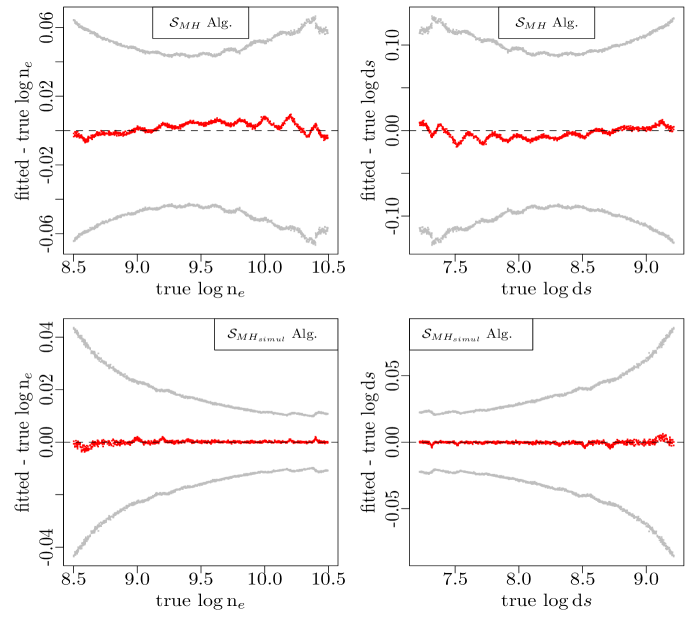
Figure 12: Comparison of best-fit values and actual input for the simulated dataset. The comparisons are shown for both $\log n_{e}$ (left column) and $\log ds$ (right column). Calculations are performed using fully Bayesian two-step MC with MH for each pixel dataset separately (top row) and for all the pixel datasets simultaneously (bottom row). The red dots represent the difference between the best-fit value and the actual input and the horizontal dashed lines represent the line of equality. The grey dots represent a vertical error of $\pm{1}$ standard deviation for the fitted values that incorporates atomic data uncertainty. Notice that the uncertainties are reduced when all the $K$-pixel datasets are used simultaneously.

The results in Figure 12 compare the fitted value using two-step MC with MH to the true value of both parameters $\log n_{e}$ (right) and $\log ds$ (left) via both separate pixel-by-pixel (top row) and simultaneous (bottom row) analyses. The grey lines represent the vertical error of one standard deviation. The dashed line represents equality, where the fitted value is identical to the true value. Compared with the separate pixel-by-pixel analyses, it shows that the error bars are smaller around the truth when we use the simultaneous analysis than when we use one pixel dataset at a time. The results in the plots illustrate that as more data are used in the analysis by simultaneously analyzing those pixels, incorporating the uncertainty in the atomic physics calculations results in more accurate fitted values.

Appendix E Appendix E

E.1 Comparison of Algorithms and Output Data Analysis

To obtain a MC sample of the parameters, $\log n_{ek}$ and $\log ds_{k}$, via the separate pixel-by-pixel analyses with joint posterior distribution in Eq (10), three algorithms were implemented for the fully Bayesian model on each of the $1000$ pixel observed datasets: $\mathcal{S}_{G}$ in Appendix B.1, $\mathcal{S}_{MH}$ in Section 5.5.3, and $\mathcal{H}$ in Appendix C.1.

Our aim is to find which algorithm provides a more accurate simulation to the target posterior distribution and is the best to be used to make statistical inference. From a statistical point of view, we assume the HMC, which might give the best result, as the base line, and to see whether these two two-step MC samplers provide better inference or not.

The first test statistic we consider is $z$-statistic, which is the difference in posterior mean between the sample values from $\mathcal{S}_{G}$ or $\mathcal{S}_{MH}$ and from $\mathcal{H}$ divided by the standard deviation of $\mathcal{H}$ because HMC is assumed to be the base line, indicating how far away that estimate is from the mean in standard units, i.e.,

$$z_{\mathrm{score}}^{i}=\frac{\mathrm{mean}_{\mathcal{S}_{i}}-\mathrm{mean}_{\mathcal{H}}}{\mathrm{sd}_{\mathcal{H}}},\ \text{for}\ i=G\text{ or }MH.$$ (E1)

Figure 13 shows the histograms of $z$-scores for both parameters, $\log n_{e}$ (top row) and $\log ds$ (bottom row), in two comparisons (left column: $\mathcal{S}_{G}$ to $\mathcal{H}$, right column: $\mathcal{S}_{MH}$ to $\mathcal{H}$) respectively considering all the $1000$ pixels. Looking at the worst case scenarios, the most extremes we see from the comparison on the left-hand side is about $0.12$ to $0.25$ of standard deviation off, which corresponds to Pixel $36$, $87$, $302$, $453$, $650$, and $934$. The comparison on the right-hand side indicates the most extremes are about $0.15$ of standard deviation off occurring at Pixel $302$ and $364$. The vertical lines correspond to the $z$-scores values of these extracted pixels. It suggests that we need to look at the full posterior distributions for those extreme pixels and for the three algorithms more closely, which will be found in Appendix E.3, to get some insights.

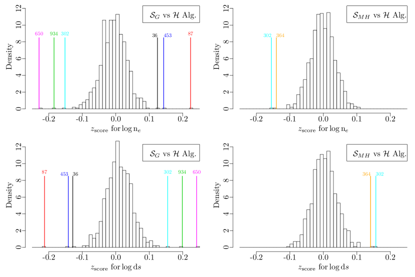
Figure 13: Selecting the extreme pixels via $z$-scores (unit difference in posterior mean) which are computed using the outputs of the three algorithms, $\mathcal{S}_{G}$, $\mathcal{S}_{MH}$, and $\mathcal{H}$ under fully Bayesian method and separate pixel-by-pixel analyses. The histograms represent the $z$-scores for both parameters, $\log n_{e}$ (top row) and $\log ds$ (bottom row), in two comparisons (left: $\mathcal{S}_{G}$ to $\mathcal{H}$, right: $\mathcal{S}_{MH}$ to $\mathcal{H}$) respectively considering all the $1000$ pixels. The vertical lines correspond to the values of pixel indices, top left: $650,934,302,36,453,87$, top right: $302,364$, bottom left: $87,453,36,302,934,650$, bottom right: $364,302$, from left to right.

The second test statistic to compare is the ratio of standard deviations between $\mathcal{S}_{G}$ or $\mathcal{S}_{MH}$ and $\mathcal{H}$, i.e.,

$$\frac{\mathrm{sd}_{\mathcal{S}_{i}}}{\mathrm{sd}_{\mathcal{H}}},\ \text{for}\ i=G\text{ or }MH,$$ (E2)

which essentially gives the relative size of confidence intervals that we compute.

Figure 14 shows the histograms of the ratio of standard deviations for both parameters, $\log n_{e}$ (top row) and $\log ds$ (bottom row), in two comparisons (left column: $\mathcal{S}_{G}$ to $\mathcal{H}$, right column: $\mathcal{S}_{MH}$ to $\mathcal{H}$) respectively considering all the $1000$ pixels. The most extremes we see from the comparison on the left-hand side corresponds to Pixel $634$ and $779$. The comparison on the right-hand side indicates the most extremes occurring at Pixel $396$, $418$, $634$, and $779$. The vertical lines correspond to the ratio values of these extracted pixels. An example of their posterior distributions for the three algorithms can be found in Appendix E.3.

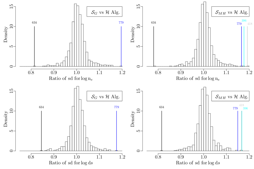
Figure 14: Selecting the extreme pixels via the ratio of standard deviations which are computed using the outputs of the three algorithms, $\mathcal{S}_{G}$, $\mathcal{S}_{MH}$, and $\mathcal{H}$ under fully Bayesian method and separate pixel-by-pixel analyses. The histograms represent the ratio of standard deviations for both parameters, $\log n_{e}$ (top row) and $\log ds$ (bottom row), in two comparisons (left: $\mathcal{S}_{G}$ to $\mathcal{H}$, right: $\mathcal{S}_{MH}$ to $\mathcal{H}$) respectively considering all the $1000$ pixels. The vertical lines correspond to the values of pixel indices, top left: $634,779$, top right: $634,779,396,418$, bottom left: $634,779$, bottom right: $634,779,418,396$, from left to right.

E.2 Parallelization

To improve the efficiency of the code, we parallelize the $1000$ pixels into $20$ or $10$ completely separate processes when pre-processing emissivities (i.e., obtaining the posterior probability of each emissivity curve) or sampling $\theta$, for all the three algorithms. The $\mathrm{doParallel}$ package is used to provide a mechanism to execute $\mathrm{foreach}$ loops in parallel within each process, where a multi-core backend is registered and a four worker cluster (of a $64$-bit $2.5$ GHz CPU with $128$ GB of RAM) is created and used. Specifically, in the source builds, we set the number of processors to use for the build to the number of cores on our machine we want to devote to the build, which is thirty-two. We also set the maximum allowed number of additional R processes allowed to be run in parallel to the current R processes, which is thirty-two as well. For $\mathcal{H}$, each pixel is run with multiple cores and four pixels are run at the same time. For $\mathcal{S}_{G}$ or $\mathcal{S}_{MH}$, we run each pixel with a different core and thirty-two multi-core backends are used in parallel.

E.3 The posterior values of the parameters for the three algorithms and for the extracted pixels

By comparing the three algorithms using the two test statistics mentioned in Appendix E.1, several extreme pixels are picked out from each comparison.

Figure 15 show the histograms of the posterior values of the parameters $\log n_{e}$ (left) and $\log ds$ (right) conditional on all $1000$ emissivity curves and the certain extracted pixel dataset respectively. The sampling algorithms used are $\mathcal{S}_{G}$ algorithm (top row), $\mathcal{S}_{MH}$ algorithm (middle row), and $\mathcal{H}$ algorithm (bottom row). Three more synthetic emissivity curves are conditioned when using $\mathcal{H}$ as described in Appendix C.3.

For Pixel $364$ (the left panel of Figure 15), which are extracted from the right column of Figure 13, having used the synthetic emissivity curves, it is still not very great job of jumping between the modes for $\mathcal{H}$ algorithm in this bimodal case.

For Pixel $396$ (the middle panel of Figure 15), it is the histograms of $\mathcal{H}$ algorithm that does not quite get into the tail that makes the standard deviation from $\mathcal{H}$ algorithm relatively small and filters this pixel out from the right column of Figure 14.

Similarly, for Pixel $650$ (the right panel of Figure 15), which are extracted from the left column of Figure 13, the $\mathcal{S}_{G}$ algorithm does not do a great job at recovering the actual posterior with a noticeable discrepancy in the mode.

       

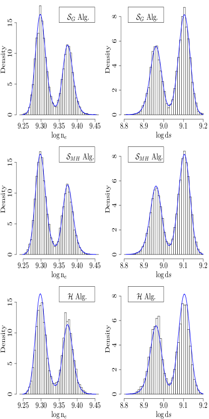
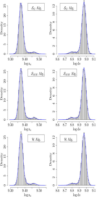
Figure 15: Selecting the optimal algorithm from the full posterior distribution for the selected extreme pixels under fully Bayesian method. The histograms represent the posterior distributions of $\log n_{e}$ (left column of each panel) and $\log ds$ (right column of each panel) conditional on all $1000$ emissivity curves and Pixel $\mathbf{364}$ (left panel), or $\mathbf{396}$ (medium panel), or $\mathbf{650}$ (right panel) in real observed data set respectively. The sampling algorithms compared are $\mathcal{S}_{G}$ (first row), $\mathcal{S}_{MH}$ (second row), and $\mathcal{H}$ (third row). The actual conditional posterior distributions for each parameter are shown as the blue lines.

E.4 Discussion

As an example of the posterior distribution of emissivity curves given Pixel $593$, we get these two dominant emissivity curves from both two-step MC samplers and HMC. Considering the two of them, it is nearly all the probability up to $0.99$, as is shown in Table 6.

Table 6: The posterior probability of the two dominant emissivity curves given Pixel $593$ using two-step MC and HMC via separate pixel-by-pixel analyses under fully Bayesian method

m	HMC with Stan ($\mathcal{H}$)	2stepMC with $\mathcal{S}_{G}$ or $\mathcal{S}_{MH}$
471	0.860	0.894
368	0.138	0.105
others	$<0.0019$	$<0.0016$

The computation time, in the realistic case, over all 1000 pixels for the three algorithms are shown in Table 7. Two ways of measuring the computation time are included, the elapsed time and the sum of user and system times. Moreover, the computation time of both two-step MC samplers consist of both quadrature part and sampling part, where the computation times of quadrature part is $1.2$ hours for both measurements.

Table 7: Computation time for the three algorithms in realistic case under fully Bayesian method and separate pixel-by-pixel analyses

Algorithm	Elaplsed (h)	Sum of User$\&$System (h)
$\mathcal{S}_{MH}$	$14.5$	$41.0$
$\mathcal{S}_{G}$	$8.0$	$20.7$
$\mathcal{H}$	$51.4$	$135.5$

We actually have two basic strategies for obtaining a MC sample from the joint posterior distribution, HMC and two-step MC sampler. By comparing the histograms of the posterior values, there is definitely an issue with the Gaussian assumption (two-step MC with Gaussian approximation) where the MC samplers are not matching very well with the actual posterior and it is more conservative. HMC algorithm looks appropriate but occasionally does not give the relative size of the mode right, though after adding synthetic emissivity curves. For all 1000 pixels, the MC samplers generated from two-step MC with MH match the density line of actual posterior very well and this algorithm takes moderate computation time. Therefore, more accurate and significantly faster, two-step MC with MH would be the best to use to make statistical inference.

In our experiment, there are $J=7$ spectral lines with corresponding wavelengths being considered, whereas two of them are not close to others in wavelength, $196.525$ and $209.916$ vs $200.021$-$203.826\ \mathring{\text{A}}$, and we call them extreme wavelengths. We have experimented with one of the two-mode-case pixels (Pixel 593), where the two extreme wavelengths are removed one at a time from the analysis and the three algorithms mentioned in Section 5.5.3, Appendix B.1, and Appendix C.1 are repeated. Whether we consider the two extreme wavelengths or not, the resulting MC samplers have a good match to their actual posterior distributions; however, the shape of the actual posterior distribution differs dramatically when including wavelength $196.525\mathring{\text{A}}$ compared to when it is excluded from the analysis. Because including the extreme wavelengths did not impact the ability of the MC samplers to recover the actual posterior distributions, we used the seven-wavelength dataset in all the experiments.

References

- Aggarwal & Keenan (2005) Aggarwal, K. M., & Keenan, F. P. 2005, A&A, 429, 1117
- Badnell et al. (2016) Badnell, N. R., Del Zanna, G., Fernández-Menchero, L., et al. 2016, Journal of Physics B Atomic Molecular Physics, 49, 094001
- Bautista et al. (2013) Bautista, M. A., Fivet, V., Quinet, P., et al. 2013, ApJ, 770, 15
- Berger et al. (1999) Berger, T. E., de Pontieu, B., Fletcher, L., et al. 1999, Sol. Phys., 190, 409
- Carpenter et al. (2016) Carpenter, B., Gelman, A., Hoffman, M., et al. 2016, Journal of Statistical Software, 20, 1
- Chung et al. (2016) Chung, H.-K., Braams, B. J., Bartschat, K., et al. 2016, Journal of Physics D Applied Physics, 49, 363002
- Culhane et al. (2007) Culhane, J. L., Harra, L. K., James, A. M., et al. 2007, Sol. Phys., 60
- Del Zanna (2011) Del Zanna, G. 2011, A&A, 533, A12
- Del Zanna (2012a) —. 2012a, A&A, 546, A97
- Del Zanna (2012b) —. 2012b, A&A, 537, A38
- Del Zanna (2013) —. 2013, A&A, 558, A73
- Del Zanna et al. (2004) Del Zanna, G., Berrington, K. A., & Mason, H. E. 2004, A&A, 422, 731
- Del Zanna et al. (2015) Del Zanna, G., Dere, K. P., Young, P. R., Landi, E., & Mason, H. E. 2015, A&A, 582, A56
- Del Zanna & Mason (2014) Del Zanna, G., & Mason, H. E. 2014, A&A, 565, A14
- Del Zanna & Storey (2012) Del Zanna, G., & Storey, P. J. 2012, A&A, 543, A144
- Dere et al. (1997) Dere, K. P., Landi, E., Mason, H. E., Monsignori Fossi, B. C., & Young, P. R. 1997, A&AS, 125, 149
- Eissner et al. (1974) Eissner, W., Jones, M., & Nussbaumer, H. 1974, Computer Physics Communications, 8, 270
- Fletcher & De Pontieu (1999) Fletcher, L., & De Pontieu, B. 1999, ApJ, 520, L135
- Foster et al. (2010) Foster, A. R., Smith, R. K., Brickhouse, N. S., Kallman, T. R., & Witthoeft, M. C. 2010, Space Sci. Rev., 157, 135
- Freeland & Handy (1998) Freeland, S. L., & Handy, B. N. 1998, Sol. Phys., 182, 497
- Gilks et al. (1996) Gilks, W. R., Richardson, S., & Spiegelhalter, D. J. 1996, Markov chain Monte Carlo in practice, 1, 19
- Gupta & Tayal (1998) Gupta, G. P., & Tayal, S. S. 1998, ApJ, 506, 464
- Hastings (1970) Hastings, W. K. 1970, Biometrika, 57, 97
- Jönsson et al. (2017) Jönsson, P., Gaigalas, G., Rynkun, P., et al. 2017, Atoms, 5, 16
- Kallman & Palmeri (2007) Kallman, T. R., & Palmeri, P. 2007, Reviews of Modern Physics, 79, 79
- Lee et al. (2011) Lee, H., Kashyap, V. L., van Dyk, D. A., et al. 2011, ApJ, 731, 126
- Loch et al. (2013) Loch, S., Pindzola, M., Ballance, C., et al. 2013, in American Institute of Physics Conference Series, Vol. 1545, American Institute of Physics Conference Series, ed. J. D. Gillaspy, W. L. Wiese, & Y. A. Podpaly, 242–251
- Luridiana & García-Rojas (2012) Luridiana, V., & García-Rojas, J. 2012, in IAU Symposium, Vol. 283, IAU Symposium, 139–143
- Mariska (1992) Mariska, J. T. 1992, The Solar Transition Region, 290
- Martens et al. (2000) Martens, P. C. H., Kankelborg, C. C., & Berger, T. E. 2000, ApJ, 537, 471
- Peres et al. (1994) Peres, G., Reale, F., & Golub, L. 1994, ApJ, 422, 412
- Schrijver & van Ballegooijen (2005) Schrijver, C. J., & van Ballegooijen, A. A. 2005, ApJ, 630, 552
- Storey & Zeippen (2010) Storey, P. J., & Zeippen, C. J. 2010, A&A, 511, A78+
- Warren et al. (2012) Warren, H. P., Winebarger, A. R., & Brooks, D. H. 2012, ApJ, 759, 141
- Warren et al. (2008) Warren, H. P., Winebarger, A. R., Mariska, J. T., Doschek, G. A., & Hara, H. 2008, ApJ, 677, 1395
- Watanabe et al. (2009) Watanabe, T., Hara, H., Yamamoto, N., et al. 2009, ApJ, 692, 1294
- Winebarger et al. (2008) Winebarger, A. R., Warren, H. P., & Falconer, D. A. 2008, ApJ, 676, 672
- Xu et al. (2014) Xu, J., Van Dyk, D. A., Kashyap, V. L., et al. 2014, The Astrophysical Journal, 794, 97
- Young (2004) Young, P. R. 2004, A&A, 417, 785
- Young et al. (2003) Young, P. R., Del Zanna, G., Landi, E., et al. 2003, ApJS, 144, 135
- Young et al. (2009) Young, P. R., Watanabe, T., Hara, H., & Mariska, J. T. 2009, A&A, 495, 587