Power Systems Topology and State Estimation by Graph Blind Source Separation

Abstract

In this paper, we consider the problem of blind estimation of states and topology (BEST) in power systems. We use the linearized DC model of real power measurements with unknown voltage phases (i.e. states) and an unknown admittance matrix (i.e. topology) and show that the BEST problem can be formulated as a blind source separation (BSS) problem with a weighted Laplacian mixing matrix. We develop the constrained maximum likelihood (ML) estimator of the Laplacian matrix for this graph BSS (GBSS) problem with Gaussian-distributed states. The ML-BEST is shown to be only a function of the states’ second-order statistics. Since the topology recovery stage of the ML-BEST approach results in a high-complexity optimization problem, we propose two low-complexity methods to implement it: (1) Two-phase topology recovery, which is based on solving the relaxed convex optimization and then finding the closest Laplacian matrix, and (2) Augmented Lagrangian topology recovery. We derive a closed-form expression for the associated Cram$\acute{\text{e}}$r-Rao bound (CRB) on the topology matrix estimation. The performance of the proposed methods is evaluated for the IEEE-14 bus test-case system and for a random network. It is shown that, asymptotically, the state estimation performance of the proposed ML-BEST methods coincides with the oracle’s minimum mean-squared-error (MSE) state estimator, and the MSE of the topology estimation achieves the proposed CRB.

I Introduction

State estimation is a critical component of modern energy management systems (EMSs) for multiple monitoring purposes, including analysis, security, control, situational awareness, stability assessment, power market design, and optimization of electricity dispatchment [1, 2]. In the DC model, the states are the bus voltage angles, while the grid topology includes the arrangement of loads or generators, transmission lines, transformers, and the statuses of system devices. It should be noted that this definition generalizes the computer science graph theory definition, which refers to the connectivity of the graph, since here the topology also includes the weights. In currently applied systems, it is assumed that the EMS has precise knowledge of the grid topology [1], which is used for obtaining accurate state estimation. However, knowledge of grid topology may not be available and it may change over time due to failure, opening and closing of switches on power lines, and the presence of new loads and generators. For example, large-scale penetration of distributed generation results in regular topology changes due to ad-hoc connection of many plug-and-play components. Even worse, a distribution system operator usually lacks topology information, as many of the distributed energy resources do not belong to the utility [3, 4]. The topology data may also be incorrect due to malicious attacks [5, 6, 7]. Thus, methods for state estimation that are not based on a known topology are crucial for obtaining a reliable system model and high power quality. An additional use for topology identification is event detection, such as identifying faults, line outages, and system imbalances [8, 9]. Moreover, it can be used to secure the system from potential cyberattacks on the topology information and to identify the potential vulnerabilities of a power system.

Several approaches to topology identification have been proposed in the literature. Detecting topological changes has been studied in [10, 11] and the conditions for the detectability of topology errors are studied in [12]. Recently, a few papers have addressed blind estimation of the grid topology by observing multiple power injection supervisory control and data acquisition (SCADA) measurements [13, 14], voltage and power data obtained by phasor measurement units (PMUs) [15, 16], voltage measurements and their associated correlations [17], and electricity price based market data [18]. In [19], an unobservable attack is designed based on incomplete knowledge of the system matrix, which is learned via a blind identification approach. The methods proposed in [13, 14, 18, 19] can reveal part of the grid topology, such as the grid connectivity and the eigenvectors of the topology matrix, but they cannot reconstruct the full topology matrix with exact scaling and true eigenvalues. Thus, incorporating blind source separation (BSS) techniques with the specific characteristics of a graph seems promising.

BSS methods aim at restoring a set of unknown source signals from a set of observed linear mixtures of these source signals (see, e.g. [20, 21, 22, 23, 24, 25, 26, 27, 28, 29]), without prior knowledge of the sources and the mixing system. The problem of BSS has been extensively investigated in the literature in the recent two decades. Prior works on maximum likelihood (ML) separation in BSS deal with general stationary sources [21, 30], autoregressive (AR) sources, and AR Gaussian mixture model distributed sources [28, 29]. The ML BSS for nonstationary structures with varying variance-profiles was considered in [31]. However, classical BSS solutions are ambiguous in the sense that the order, signs and scales of the original signals cannot be retrieved. These ambiguities cannot be tolerated in the considered power system problem. In addition, usually the distributions of the states are assumed to be Gaussian due to the central limit theorem, while most BSS methods cannot handle Gaussian sources. Therefore, new methods for BSS are required for the semiblind scenario of a Laplacian mixing matrix with Gaussian sources, without permutation and scaling problems.

In addition to state estimation in power systems, the recent field of graph signal processing (GSP) [32] has many applications, [33, 34, 35]. A major challenge in GSP is learning the graph structure from data under Laplacian matrix constraints (see, e.g. [36, 37, 38]) and blind deconvolution of signals on graphs [39], aim to jointly identify the filter coefficients and the input signal. In future work the recent approach has the potential to be extended to general GSP applications.

In this paper, we consider the problem of state estimation and topology identification in power systems based on active power measurements. First, we show that this problem is equivalent to the problem of BSS with a weighted Laplacian mixing matrix, where the weights are determined by the branch susceptances. Then, we derive the ML blind estimation of states and topology (ML-BEST) method for Gaussian-distributed states, that incorporates the constraints of a Laplacian mixing matrix and is shown to be a second-order statistics (SOS) method. Since the topology recovery stage of the ML-BEST estimator is shown to be a NP-hard optimization problem, we suggest two practical low-complexity methods to implement this stage: (1) Two-Stage topology recovery, which is based on solving the relaxed convex optimization and then finding the closest Laplacian matrix, and (2) Augmented Lagrangian topology recovery. Preliminary results can be found in [40]. We also derive a closed-form expression for the Cram$\acute{\text{e}}$r-Rao bound (CRB). Finally, simulations demonstrate that the proposed ML-BEST methods are applicable for different network topologies, and asymptotically achieve the CRB.

The remainder of the paper is organized as follows. In Section II we introduce the system model and the graph BSS (GBSS) problem for state and topology estimation in power systems. The ML-BEST solution is defined and two different practical methods for its topology recovery stage are suggested in Sections III and IV, respectively. Section V offers some remarks, including a parameter identifiability analysis, complexity discussion, and possible extensions of the proposed model and methods. A closed-form expression for the CRB of the topology matrix is derived in Section VI. The proposed methods are evaluated via simulations in Section VII. Conclusions appear in Section VIII.

II Problem formulation

In this section, we formulate the problem of estimating the state and topology/admittance matrix in power systems under the linear DC power model. We show that this problem is equivalent to BSS with a Laplacian mixing matrix.

II-A Notation

In the rest of this paper vectors are denoted by boldface lowercase letters and matrices by boldface uppercase letters. The $K\times K$ identity matrix is denoted by ${\bf{I}}_{K}$, and ${\mathbf{1}}_{K}$ denotes the constant $K$-length one vector. The vectors ${\bf{0}}$ and ${\bf{e}}_{m}$ are zero vectors (with appropriate dimension), except for the $m$th element of ${\bf{e}}_{m}$, which is $1$. Additionally, $\delta_{m,k}$ denotes Kronecker’s delta, which equals $1$ if $m=k$ and $0$ otherwise. The notations $|\cdot|$, ${\text{Tr}}\{\cdot\}$, and $\otimes$ denote the determinant operator, the trace operator, and the Kronecker product, respectively. For a full-rank matrix ${\bf{A}}$, ${\bf{A}}^{\dagger}\stackrel{{\scriptstyle\triangle}}{{=}}\left({\bf{A}}^{T}{\bf{A}}\right)^{-1}{\bf{A}}^{T}$ is the Moore-Penrose pseudo-inverse. The $m$th element of the vector ${\bf{a}}$, the $(m,q)$th element of the matrix ${\bf{A}}$, and the $(m_{1}:m_{2}\times q_{1}:q_{2})$ submatrix of ${\bf{A}}$ are denoted by $a_{m}$, ${\bf{A}}_{m,q}$, and ${\bf{A}}_{m_{1}:m_{2},q_{1}:q_{2}}$, respectively. If ${\bf{A}}$ is a positive semidefinite matrix we denote it by ${\bf{A}}\succeq{\bf{0}}$ and its square root, ${\bf{A}}^{\frac{1}{2}}$, satisfies ${\bf{A}}^{\frac{1}{2}}{\bf{A}}^{\frac{1}{2}}={\bf{A}}$, where ${\bf{A}}^{-\frac{1}{2}}$ denotes the inverse of this square root. For any matrix ${\bf{A}}$, $||{\bf{A}}||_{F}$ and $||{\bf{A}}||_{0}$ denote its Frobenius and $\ell_{0}$-(pseudo)norm (counting its non-zero entries), respectively, $\{{\bf{A}}\}^{+}=\max\{{\bf{A}},0\}$ is the nonnegative part of ${\bf{A}}$, and ${\text{vec}}({\bf{A}})$ is a vector obtained by stacking its columns. Similarly, for any symmetric matrix ${\bf{S}}$, ${\text{vech}}({\bf{S}})$ is a vector obtained by stacking the columns of the lower triangular part of ${\bf{S}}$, including the diagonal, into a single column. Finally, we denote the cone of real symmetric matrices of size $M\times M$ by ${\mathbb{S}}^{M}$.

II-B Graph representation of power systems

A power system can be represented as an undirected connected weighted graph, ${\mathcal{G}}({\mathcal{V}},\xi)$, where the set of vertices, ${\mathcal{V}}=\{1,\ldots,M\}$, is the set of buses (that represent interconnections, generators or loads) and the edge set, $\xi$, is the set of connected transmission lines between the buses. An arbitrary orientation is assigned to each edge $e_{i}=(m,k)\in\xi$, $m,k=1,\ldots,M$, $k<m$, $i=1,\ldots,\frac{M(M-1)}{2}$, that are ordered in a lexicographical order, which connects the vertices $m$ and $k$. The cardinality of the edge set, $|{\xi}|=\frac{M(M-1)}{2}$, represents all possible connections in the graph. According to the $\pi$-model of transmission lines [1], each line is characterized by the line admittance $Y_{m,k}$, $\forall(m,k)\in\xi$.

The incidence matrix of a graph is ${\bf{B}}\in{\mathbb{R}}^{M\times\frac{M(M-1)}{2}}$ [35], where the $(m,i)$ element of ${\bf{B}}$ is given by

$${\bf{B}}_{m,i}=\left\{\begin{array}[]{ll}1&e_{i}=(m,k){\text{ is connected, $m$ is the source}}\\ -1&e_{i}=(k,m){\text{ is connected, $k$ is the source}}\\ 0&{\text{otherwise}}\\ \end{array}\right.,$$ (4)

$\forall m=1,\ldots,M$ and $i=1,\ldots,\frac{M(M-1)}{2}$. In addition, let ${\bf{\Gamma}}\in{\frac{M(M-1)}{2}\times\frac{M(M-1)}{2}}$ be a diagonal matrix where ${\bf{\Gamma}}_{i,i}=Y_{m,k}$ if $e_{i}=(m,k)$, $i=1,\ldots,\frac{M(M-1)}{2}$. For connections that do not exist we use ${\bf{\Gamma}}_{i,i}=0$. Then, we can define the graph Laplacian matrix, ${\bf{L}}$, as

$${\bf{L}}\stackrel{{\scriptstyle\triangle}}{{=}}{\bf{B}}{\bf{\Gamma}}{\bf{B}}^{T}.$$ (5)

The matrix ${\bf{L}}\in{\mathbb{R}}^{M\times M}$ is a real, symmetric, and positive semidefinite matrix, which satisfies the null space property, ${\bf{L}}\mathbf{1}_{M}={\bf{0}}$, and with nonpositive off-diagonal elements.

II-C DC model and problem formulation

We consider the DC power flow model [1], which is based on the following assumptions on the network:

A.1

Branches are considered lossless, which results in $Y_{m,k}=b_{m,k}$, where $b_{m,k}$ is the susceptance of the $(m,k)$ branch.

A.2

The bus voltage magnitudes, $V_{m}$, $m=1,\ldots,M$, are approximated by 1 per unit (p.u.).

A.3

Voltage angle differences across branches are small, such that $\sin(\theta_{m}-\theta_{k})\approx\theta_{m}-\theta_{k}$, where $\theta_{m}$, $m=1,\ldots,M$, are the bus voltage angles.

Under Assumptions A.1-A.3, the active power injected at bus $m$ satisfies

$$p_{m}=-\sum\nolimits_{k=1}^{M}b_{m,k}V_{m}V_{k}\sin(\theta_{m}-\theta_{k})\hskip 39.83368pt$$

$$\approx-\sum\nolimits_{k=1}^{M}Y_{m,k}(\theta_{m}-\theta_{k}),~{}\forall m=1,\ldots,M.$$ (6)

Now, let ${\bf{p}}[n]\stackrel{{\scriptstyle\triangle}}{{=}}{[p_{1}[n],\dots,p_{M}[n]]}^{T}$ be the vector of active power injected and ${\mbox{\boldmath$\theta$}}[n]\stackrel{{\scriptstyle\triangle}}{{=}}{[\theta_{1}[n],\dots,\theta_{M}[n]]}^{T}$ the vector of voltage phase angles at time $n$, $\forall n=0,\ldots,N-1$. Then, based on the model from (II-C), the noisy linearized DC model of the network can be written as

$${\bf{p}}[n]={\bf{L}}{\mbox{\boldmath$\theta$}}[n]+{\bf{w}}[n],~{}~{}~{}n=0,\ldots,N-1,$$ (7)

where the topology matrix ${\bf{L}}$, defined in (5), is a deterministic unknown Laplacian matrix, which is considered static for a short-period of time and under normal operating conditions. The noise is a stationary Gaussian sequence with zero mean and a covariance matrix $\sigma^{2}{\bf{I}}_{M}$, i.e. ${\bf{w}}[n]\sim{\cal{N}}({\bf{0}},\sigma^{2}{\bf{I}}_{M})$, and it is assumed that the additive noises are independent of the state vectors. The vectors $\{{\mbox{\boldmath$\theta$}}[n]\}$, $n=0,\ldots,N-1$, are assumed to be unknown random states with a joint probability density function (pdf) $f_{\mbox{\boldmath{\scriptsize$\theta$}}}(\cdot)$ and marginal pdfs of $\theta_{m}$, $f_{\theta_{m}}(\cdot)$, $m=1,\ldots,M$. By subtracting the mean from the data, we can assume, without loss of generality, that $\theta$ has zero mean. The resulting centralized measurements are given by ${{\bf{p}}}[n]-\bar{{\bf{p}}}$, where $\bar{{\bf{p}}}\stackrel{{\scriptstyle\triangle}}{{=}}\frac{1}{N}\sum_{n=0}^{N-1}{{\bf{p}}}[n]$ is the sample mean. For the rest of this paper, ${{\bf{p}}}[n]$ will denote the mean-centered active power data.

Now, in order to reformulate the model with a full-rank mixing matrix, we use the relation

$${\bf{L}}={\bf{U}}\tilde{{\bf{L}}}{\bf{U}}^{T},$$ (8)

where

$${\bf{U}}\stackrel{{\scriptstyle\triangle}}{{=}}\left[\begin{array}[]{c}-{\mathbf{1}}_{M-1}^{T}\\ {\bf{I}}_{M-1}\end{array}\right]\in{\mathbb{R}}^{M\times(M-1)}$$ (9)

and $\tilde{{\bf{L}}}\stackrel{{\scriptstyle\triangle}}{{=}}{\bf{L}}_{2:M,2:M}$ is a $1$st-order reduced-Laplacian matrix, which is obtained by removing the first row and first column of ${\bf{L}}$. By substituting (8) in (7), one obtains

$${\bf{p}}[n]={\bf{U}}\tilde{{\bf{L}}}\tilde{{\mbox{\boldmath$\theta$}}}[n]+{\bf{w}}[n],~{}~{}~{}n=0,\ldots,N-1,$$ (10)

where

$$\tilde{{\mbox{\boldmath$\theta$}}}[n]\stackrel{{\scriptstyle\triangle}}{{=}}{\bf{U}}^{T}{{\mbox{\boldmath$\theta$}}}[n]=[\theta_{2}[n]-\theta_{1}[n],\ldots,\theta_{M}[n]-\theta_{1}[n]],$$

$n=0,\ldots,N-1$. By multiplying both sides of (10) with ${\bf{U}}^{\dagger}$, it can be verified that the model in (10) is equivalent to

$$\tilde{{\bf{p}}}[n]=\tilde{{\bf{L}}}\tilde{{\mbox{\boldmath$\theta$}}}[n]+\tilde{{\bf{w}}}[n],~{}~{}~{}n=0,\ldots,N-1,$$ (11)

where $\tilde{{\bf{p}}}[n]\stackrel{{\scriptstyle\triangle}}{{=}}{\bf{U}}^{\dagger}{\bf{p}}[n]$ and $\tilde{{\bf{w}}}[n]\stackrel{{\scriptstyle\triangle}}{{=}}{\bf{U}}^{\dagger}{\bf{w}}[n]$, $n=0,\ldots,N-1$. In addition, it can be shown (see, e.g. pp. 134-144 [42]) that the modified noise sequence satisfies $\tilde{{\bf{w}}}[n]\sim{\cal{N}}({\bf{0}},\sigma^{2}{\bf{U}}^{\dagger}({\bf{U}}^{\dagger})^{T})$, $n=0,\ldots,N-1$.

We assume here that all sources are time-independent Gaussian distributed, i.e. ${\mbox{\boldmath$\theta$}}[n]\sim{\cal{N}}({\bf{0}},{\mbox{\boldmath$\Sigma$}}_{\mbox{\boldmath{\scriptsize$\theta$}}})$, $n=0,\ldots,N-1$. Thus, ${\tilde{{\mbox{\boldmath$\theta$}}}}[n]\sim{\cal{N}}({\bf{0}},{\mbox{\boldmath$\Sigma$}}_{\mbox{\boldmath{\scriptsize$\tilde{\theta}$}}})$, $n=0,\ldots,N-1$, where ${\mbox{\boldmath$\Sigma$}}_{\mbox{\boldmath{\scriptsize$\tilde{\theta}$}}}\stackrel{{\scriptstyle\triangle}}{{=}}{\bf{U}}^{T}{\mbox{\boldmath$\Sigma$}}_{\mbox{\boldmath{\scriptsize$\theta$}}}{\bf{U}}$. Under the assumption that ${\mbox{\boldmath$\Sigma$}}_{\mbox{\boldmath{\scriptsize$\theta$}}}$ is known, the observations vectors are also independent Gaussian-distributed vectors, i.e. ${{\bf{p}}}[n]\sim{\cal{N}}\left({\bf{0}},{\mbox{\boldmath$\Sigma$}}_{\bf{p}}({{\bf{L}}},\sigma^{2})\right)$ and $\tilde{{\bf{p}}}[n]\sim{\cal{N}}\left({\bf{0}},{\mbox{\boldmath$\Sigma$}}_{\tilde{{\bf{p}}}}(\tilde{{\bf{L}}},\sigma^{2})\right)$, $n=0,\ldots,N-1$, where

$${\mbox{\boldmath$\Sigma$}}_{\bf{p}}({{\bf{L}}},\sigma^{2})\stackrel{{\scriptstyle\triangle}}{{=}}{{\bf{L}}}^{T}{\mbox{\boldmath$\Sigma$}}_{\mbox{\boldmath{\scriptsize$\theta$}}}{{\bf{L}}}+\sigma^{2}{\bf{I}}_{M}$$ (12)

and, assuming nonsingular matrices,

$${\mbox{\boldmath$\Sigma$}}_{\tilde{{\bf{p}}}}(\tilde{{\bf{L}}},\sigma^{2})\stackrel{{\scriptstyle\triangle}}{{=}}\tilde{{\bf{L}}}^{T}{\mbox{\boldmath$\Sigma$}}_{\mbox{\boldmath{\scriptsize$\tilde{\theta}$}}}\tilde{{\bf{L}}}+{\sigma}^{2}{\bf{U}}^{\dagger}({\bf{U}}^{\dagger})^{T}.$$ (13)

The reduced topology matrix, $\tilde{{\bf{L}}}$, has the following properties [35, 37]:

P.1

Full rank - Under the assumption of a connected graph, $\tilde{{\bf{L}}}$ is a nonsingular matrix of rank $M-1$ and, thus, can be identified in general. In power system terminology, we assume that there are no unobservable islands in the grid.

P.2

Positive semidefinite - Since ${\bf{L}}$ is a symmetric, positive semidefinte matrix, $\tilde{{\bf{L}}}$ is also a symmetric, positive semidefinte matrix.

P.3

Nonpositive off-diagonal elements - $\tilde{{\bf{L}}}_{k,m}\leq 0$, $\forall k,m=1,\ldots,M-1$, $k\neq m$.

P.4

Diagonally dominant - Since ${\bf{L}}$ is a Laplacian matrix, $\tilde{{\bf{L}}}$ is a diagonally dominant matrix, i.e. $\sum_{m=1,m\neq k}^{M-1}|\tilde{{\bf{L}}}_{k,m}|\leq|\tilde{{\bf{L}}}_{k,k}|$, $\forall k=1,\ldots,M-1$.

P.5

Sparsity (optional) - It is shown in previous works that the power system is sparse [43], i.e. the zero pseudonorm of the off-diagonal entries of $\tilde{{\bf{L}}}$, $||\tilde{{\bf{L}}}||_{0-{\text{off}}}$, is much smaller than $(M-1)(M-2)$.

III ML-BEST

In this section, we develop the basic ML-BEST approach that jointly reconstructs the matrix ${\bf{L}}$ and the states ${\mbox{\boldmath$\theta$}}[n]$, $n=0,\ldots,N-1$, for the model from Section II. This problem can be interpreted as a BSS problem with a Laplacian mixing matrix, or graph BSS (GBSS). First, in Subsection III-A the minimum mean-squared-error (MMSE) estimator of the random states, ${{\mbox{\boldmath$\theta$}}}[n]$, $n=0,\ldots,N-1$, is developed. Then, in Subsection III-C, we develop the ML estimator of the noise variance, $\sigma^{2}$, and formulate the optimization problem describing the ML estimator of the mixing system.

III-A MMSE state estimation

For given ${\bf{L}}$ and $\sigma^{2}$, the sequences ${\bf{p}}[n]$, $n=0,\ldots,N-1$, ${\mbox{\boldmath$\theta$}}[n]$, $n=0,\ldots,N-1$, are jointly Gaussian. Thus, in this case the MMSE estimator of the state vector is a linear estimator given by (see, e.g. Chapter 20 in [44], [45])

$$\hat{{\mbox{\boldmath$\theta$}}}[n]={\mbox{\boldmath$\Sigma$}}_{\mbox{\boldmath{\scriptsize$\theta$}}}{\bf{L}}\left({{\bf{L}}}^{T}{\mbox{\boldmath$\Sigma$}}_{\mbox{\boldmath{\scriptsize$\theta$}}}{{\bf{L}}}+\sigma^{2}{\bf{I}}_{M}\right)^{\dagger}{\bf{p}}[n],$$ (14)

$n=0,\ldots,N-1$. We refer to the estimator in (14) as the oracle MMSE state estimator, i.e. an ideal estimator which has perfect knowledge of the noise variance and the system topology.

The practical state estimator for the considered GBSS problem is obtained by plugging in the ML estimators of the noise variance and the reduced-Laplacian matrix, $\hat{\sigma}^{2}$ and $\hat{\tilde{{\bf{L}}}}^{\text{ML}}$, respectively, that are developed in the following in Subsections III-B and III-C, into (14), which results in

$$\hat{{{\mbox{\boldmath$\theta$}}}}[n]={\mbox{\boldmath$\Sigma$}}_{\mbox{\boldmath{\scriptsize$\theta$}}}\hat{{{\bf{L}}}}^{\text{ML}}\left(\left(\hat{{{\bf{L}}}}^{\text{ML}}\right)^{T}{\mbox{\boldmath$\Sigma$}}_{\mbox{\boldmath{\scriptsize$\theta$}}}\hat{{{\bf{L}}}}^{\text{ML}}+\hat{\sigma}^{2}{\bf{I}}_{M}\right)^{\dagger}{\bf{p}}[n],$$ (15)

$n=0,\ldots,N-1$.

For high signal-to-noise ratio (SNR) values, i.e. when $\sigma^{2}\rightarrow 0$, the matrix ${{\bf{L}}}^{T}{\mbox{\boldmath$\Sigma$}}_{\mbox{\boldmath{\scriptsize$\theta$}}}{{\bf{L}}}$ is a singular matrix and, thus, the covariance matrix of the data from (12) is also a singular matrix. In this case, instead of using pseudo inverse as in (14) and (15), the unknown parameters can also be treated by removing the linearly dependent random variable (see, e.g. Chapters 3 and 10 in [46]). In power system state estimation this is usually done by setting one bus as a reference bus and setting its angle to zero (see, e.g. [1]), and then only estimating ${\tilde{{\mbox{\boldmath$\theta$}}}}[n]$. Here we prefer to use instead the state estimation method in (14) and (15) for estimation of ${\mbox{\boldmath$\theta$}}[n]$.

III-B ML estimation of the noise variance

It is shown in [47, 48, 49] that for Gaussian measurements with the aforementioned structure, the ML estimator of the noise variance $\sigma^{2}$ is given by

$$\hat{\sigma}^{2}=\lambda_{M},$$ (16)

where $\lambda_{1}\geq\lambda_{2}\geq\ldots\geq\lambda_{M}$ are the eigenvalues of the sample covariance matrix,

$$\hat{{\mbox{\boldmath$\Sigma$}}}_{\bf{p}}\stackrel{{\scriptstyle\triangle}}{{=}}\frac{1}{N}\sum_{n=0}^{N-1}{{\bf{p}}}[n]{{\bf{p}}}^{T}[n].$$ (17)

III-C System identification: ML estimation of the mixing matrix

By using the invariance property of the ML estimator [50] and the relation in (8), the ML estimator of the full Laplacian matrix can be obtained from the ML estimator of the reduced-Laplacian matrix, $\hat{\tilde{{\bf{L}}}}^{({\text{ML}})}$, as follows:

$$\hat{{\bf{L}}}^{({\text{ML}})}={\bf{U}}\hat{\tilde{{\bf{L}}}}^{({\text{ML}})}{\bf{U}}^{T}.$$ (18)

In the following, the ML estimation of the reduced topology matrix, $\tilde{{\bf{L}}}$, is formulated and is shown to be NP-hard. Practical methods to approximate the ML estimator of $\tilde{{\bf{L}}}$, $\hat{\tilde{{\bf{L}}}}^{({\text{ML}})}$, are developed in the next section. Under the model from (11) and the Gaussian-distributed sources assumptions, the normalized log likelihood of $\tilde{{\bf{p}}}[n]$, $n=0,\ldots,N-1$, after removing constant terms and substituting the ML estimator of the noise variance from (16), satisfies

$$\psi(\tilde{{\bf{L}}})=-{\text{Tr}}\left\{\hat{{\mbox{\boldmath$\Sigma$}}}_{\tilde{{\bf{p}}}}{\mbox{\boldmath$\Sigma$}}_{\tilde{{\bf{p}}}}^{-1}(\tilde{{\bf{L}}},\hat{\sigma}^{2})\right\}-\log\left|{\mbox{\boldmath$\Sigma$}}_{\tilde{{\bf{p}}}}(\tilde{{\bf{L}}},\hat{\sigma}^{2})\right|,$$ (19)

where

$$\hat{{\mbox{\boldmath$\Sigma$}}}_{\tilde{{\bf{p}}}}\stackrel{{\scriptstyle\triangle}}{{=}}\frac{1}{N}\sum_{n=0}^{N-1}\tilde{{\bf{p}}}[n]\tilde{{\bf{p}}}^{T}[n]={\bf{U}}^{\dagger}\hat{{\mbox{\boldmath$\Sigma$}}}_{{{\bf{p}}}}({\bf{U}}^{\dagger})^{T}$$ (20)

is the modified sample covariance matrix and the last equality is obtained by substituting (17). That is, the log-likelihood from (19) depends on the data only through the sample covariance matrix, $\hat{{\mbox{\boldmath$\Sigma$}}}_{\tilde{{\bf{p}}}}$, which is the sufficient statistic for estimating $\tilde{{\bf{L}}}$.

Since the reduced-Laplacian matrix satisfies Properties P.1-P.4, we are interested in minimizing $-\psi(\tilde{{\bf{L}}})$ over the domain of symmetric matrices and under the associated constraints as follows:

$$\begin{array}[]{l}\min\limits_{\tilde{{\bf{L}}}\in{\mathbb{S}}^{M-1}}-\psi(\tilde{{\bf{L}}})\\ {\text{ such that }}\\ 1)~{}\tilde{{\bf{L}}}\succ{\bf{0}}\\ 2)~{}{\tilde{{\bf{L}}}}_{m,k}\leq 0,~{}~{}~{}\forall m,k=1,\ldots,M-1,~{}k<m\\ 3)~{}\sum_{k=1}^{M-1}\tilde{{\bf{L}}}_{m,k}\geq 0,~{}~{}~{}\forall m=1,\ldots,M-1\end{array}.$$ (26)

The Gaussian log-likelihood function, $\psi(\tilde{{\bf{L}}})$, is a concave function of the inverse covariance matrix, ${\mbox{\boldmath$\Sigma$}}_{\tilde{{\bf{p}}}}^{-1}(\tilde{{\bf{L}}},\hat{\sigma}^{2})$. However, even without the sparsity constraint, the constraints in (26) cannot be rewritten as convex constraints on ${\mbox{\boldmath$\Sigma$}}_{\tilde{{\bf{p}}}}^{-1}(\tilde{{\bf{L}}},\hat{\sigma}^{2})$. Therefore, the resulting optimization is not a convex optimization and, in addition, a direct Karush-Kuhn-Tucker (KKT) conditions [51] solution of this constrained minimization is intractable. Two low-complexity implementation methods are described in the next section.

Imposing directly the sparsity constraint in P.5 usually results in complex combinatorial searches, and following advances in compressive sensing [52, 53], the sparsity constraint can be approximated by restricting the off-diagonal $\ell_{1}$-norm. We perform simulations that suggest that simple elementwise thresholding of the estimated Laplacian matrix is competitive with $\ell_{1}$ methods. Thus, at the end of the ML-BEST approach, we thresholded the off-diagonal elements of the estimator of the topology matrix, $\hat{{\bf{L}}}^{({\text{ML}})}$, from (18), with a threshold, $\tau$, such that the $(k,m)$th element of the final estimation is given by

$$\hat{{{{\bf{L}}}}}^{({\text{ML}})}_{k,m}=\left\{\begin{array}[]{lr}\hat{{{{\bf{L}}}}}^{({\text{ML}})}_{k,m}&{\text{if }}|\hat{{{{\bf{L}}}}}^{({\text{ML}})}_{k,m}|>\tau\\ 0&{\text{otherwise}}\end{array}\right.,$$ (29)

$k,m=1,\ldots,M-1$, $k\neq m$. The threshold $\tau$ should be tuned until the desired level of sparsity is achieved, while keeping connectivity. The diagonal elements of ${{\bf{L}}}$ are known to be positive for the Laplacian matrix, which thus, has partially known support. Thus, $\tau$ set to be smaller than the magnitude of the smallest estimated element of the diagonal:

$$\tau=\alpha\min_{m=1,\ldots,M}\hat{{{{\bf{L}}}}}^{({\text{ML}})}_{m,m},$$ (30)

where $0<\alpha<1$. The value of $\alpha$ can be set to the inverse of the number of buses, $\frac{1}{M}$, or of the average nodal degree [35].

The basic ML-BEST algorithm is summarized in Algorithm 1, for any method of estimation of the reduced-Laplacian matrix, ${\tilde{{\bf{L}}}}$. Two such methods are described in Section IV.

Input: • Observations ${\bf{p}}[n]$, $n=0,\ldots,N-1$. • State covariance matrix, ${\mbox{\boldmath$\Sigma$}}_{\tilde{\theta}}$. Output: Estimators $\hat{{\bf{L}}}$ and $\hat{{\mbox{\boldmath$\theta$}}}[n]$, $n=0,\ldots,N-1$.

Algorithm Steps:

1. (Optional) Remove the sample mean, $\bar{{\bf{p}}}\stackrel{{\scriptstyle\triangle}}{{=}}\frac{1}{N}\sum_{n=0}^{N-1}{{\bf{p}}}[n]$, from the observations ${\bf{p}}[n]$, $n=0,\ldots,N-1$.

2. Obtain the sample covariance matrix, $\hat{{\mbox{\boldmath$\Sigma$}}}_{\bf{p}}$, by (17).

3. Perform eigendecomposition operation for the sample covariance matrix $\hat{{\mbox{\boldmath$\Sigma$}}}_{\bf{p}}$ to find its eigenvalues $\lambda_{1}\geq\lambda_{2}\geq\ldots\geq\lambda_{M}$.

4. Estimate the noise variance by the smallest eigenvalue, $\hat{\sigma}^{2}=\lambda_{M}$.

5. Estimate the reduced-Laplacian matrix and obtain approximation to $\hat{\tilde{{\bf{L}}}}^{({\text{ML}})}$, for example, by the two-phase/augmented ML-BEST from Section IV.

6. Reconstruct the full topology matrix according to (18):

   $$\hat{{\bf{L}}}^{({\text{ML}})}={\bf{U}}\hat{\tilde{{\bf{L}}}}^{({\text{ML}})}{\bf{U}}^{T}.$$

7. Impose sparsity by setting the threshold according to (30):

   $$\tau=\alpha\min_{m=1,\ldots,M}\hat{{{{\bf{L}}}}}^{({\text{ML}})}_{m,m}$$

   and thresholding such that the $(k,m)$th element of the final estimation is given by (29):

   $$\hat{\tilde{{{\bf{L}}}}}^{({\text{ML}})}_{k,m}=\left\{\begin{array}[]{lr}\hat{\tilde{{{\bf{L}}}}}^{({\text{ML}})}_{k,m}&{\text{if }}|\hat{\tilde{{{\bf{L}}}}}^{({\text{ML}})}_{k,m}|>\tau\\ 0&{\text{otherwise}}\end{array}\right.,$$

   $k,m=1,\ldots,M-1$, $k\neq m$.

8. Evaluate the sources according to (15):

   $$\hat{{{\mbox{\boldmath$\theta$}}}}[n]={\mbox{\boldmath$\Sigma$}}_{\mbox{\boldmath{\scriptsize$\theta$}}}\hat{{{\bf{L}}}}^{\text{ML}}\left(\left(\hat{{{\bf{L}}}}^{\text{ML}}\right)^{T}{\mbox{\boldmath$\Sigma$}}_{\mbox{\boldmath{\scriptsize$\theta$}}}\hat{{{\bf{L}}}}^{\text{ML}}+\hat{\sigma}^{2}{\bf{I}}_{M}\right)^{\dagger}{\bf{p}}[n],$$

   $n=0,\ldots,N-1$.

Algorithm 1 Basic ML-BEST Algorithm

IV Practical implementations of the ML-BEST

In this section, two low-complexity estimation methods of the reduced topology are derived: 1) Two-Stage topology recovery in Subsection IV-A; and 2) Augmented Lagrangian topology recovery in Subsection IV-B.

IV-A Two-phase topology recovery

In this subsection, we propose a low-complexity method for solving (26) in two phases. First, we relax the original optimization problem from (26), by removing constraints $2)$ and $3)$ into

$$\begin{array}[]{l}\min\limits_{\tilde{{\bf{L}}}\in{\mathbb{S}}^{M-1}}-\psi(\tilde{{\bf{L}}}){\text{ such that }}1)~{}\tilde{{\bf{L}}}\succeq{\bf{0}}\end{array}.$$ (32)

It is well known that the relaxed optimization problem from (32) is a convex optimization w.r.t. ${{\mbox{\boldmath$\Sigma$}}}_{\tilde{{\bf{p}}}}^{-1}(\tilde{{\bf{L}}},\hat{\sigma}^{2})$ and the optimal solution is the sample covariance matrix inverse, $\hat{{\mbox{\boldmath$\Sigma$}}}_{\tilde{{\bf{p}}}}^{-1}$, under the assumption of nonsingular matrices (see, e.g. p. 466 in [54], [55]). Then, by using the invariance property of the ML estimator [50], the one-to-one mapping in (13), and the symmetry $\tilde{{\bf{L}}}^{T}=\tilde{{\bf{L}}}$, one obtains that the unique minimum of (32) w.r.t. $\tilde{{\bf{L}}}$ , which is the ML estimator of a symmetric positive definite mixing matrix, $\hat{\tilde{{\bf{L}}}}^{\text{PD}}$, satisfies

$$\hat{{\mbox{\boldmath$\Sigma$}}}_{\tilde{{\bf{p}}}}=\hat{\tilde{{\bf{L}}}}^{\text{PD}}{\mbox{\boldmath$\Sigma$}}_{\mbox{\boldmath{\scriptsize$\tilde{\theta}$}}}\hat{\tilde{{\bf{L}}}}^{\text{PD}}+\hat{\sigma}^{2}{\bf{U}}^{\dagger}({\bf{U}}^{\dagger})^{T},$$ (33)

which implies that

$$\hat{\tilde{{\bf{L}}}}^{\text{PD}}={\mbox{\boldmath$\Sigma$}}_{\mbox{\boldmath{\scriptsize$\tilde{\theta}$}}}^{-\frac{1}{2}}\left({\mbox{\boldmath$\Sigma$}}_{\mbox{\boldmath{\scriptsize$\tilde{\theta}$}}}^{\frac{1}{2}}\left(\hat{{\mbox{\boldmath$\Sigma$}}}_{\tilde{{\bf{p}}}}-\hat{\sigma}^{2}{\bf{U}}^{\dagger}({\bf{U}}^{\dagger})^{T}\right){\mbox{\boldmath$\Sigma$}}_{\mbox{\boldmath{\scriptsize$\tilde{\theta}$}}}^{\frac{1}{2}}\right)^{\frac{1}{2}}{\mbox{\boldmath$\Sigma$}}_{\mbox{\boldmath{\scriptsize$\tilde{\theta}$}}}^{-\frac{1}{2}}.$$ (34)

In the second phase, we find the closest graph Laplacian matrix to the matrix ${\bf{U}}\hat{\tilde{{\bf{L}}}}^{\text{PD}}{\bf{U}}^{T}$ in the sense of Frobenius norm. Thus, we solve the following optimization problem:

$$\begin{array}[]{l}\min\limits_{{{\bf{L}}}\in{\mathbb{S}}^{M}}||{\bf{U}}\hat{\tilde{{\bf{L}}}}^{\text{PD}}{\bf{U}}^{T}-{\bf{L}}||_{F}\\ {\text{ such that }}\\ 1)~{}{{\bf{L}}}\succeq{\bf{0}}\\ 2)~{}{{\bf{L}}}_{m,k}\leq 0,~{}~{}~{}\forall m,k=1,\ldots,M,~{}k<m\\ 3)~{}\sum_{k=1}^{M}{{\bf{L}}}_{m,k}=0,~{}~{}~{}\forall m=1,\ldots,M\end{array}.$$ (40)

The problem in (40) is a convex optimization problem and can be efficiently computed by standard semidefinite program solvers, such as CVX [56]. This two-phase topology recovery algorithm is summarized in Algorithm 2. The ML-BEST approach with two-phase topology recovery is implemented by Algorithm 1, where Step 5 is implemented by Algorithm 2.

Input: ${\mbox{\boldmath$\Sigma$}}_{\mbox{\boldmath{\scriptsize$\tilde{\theta}$}}}$, $\hat{{\mbox{\boldmath$\Sigma$}}}_{{{\bf{p}}}}$, $\hat{\sigma}^{2}$.

Output: Estimator $\hat{\tilde{{\bf{L}}}}^{\text{ML}}$.

Algorithm Steps:

1. Evaluate the reduced sample covariance matrix from (20) by $\hat{{\mbox{\boldmath$\Sigma$}}}_{\tilde{{\bf{p}}}}={\bf{U}}^{\dagger}\hat{{\mbox{\boldmath$\Sigma$}}}_{{{\bf{p}}}}({\bf{U}}^{\dagger})^{T}$.

2. Evaluate the optimal solution of the optimization in (32) by (34):

   $$\hat{\tilde{{\bf{L}}}}^{{\text{PD}}}={\mbox{\boldmath$\Sigma$}}_{\mbox{\boldmath{\scriptsize$\tilde{\theta}$}}}^{-\frac{1}{2}}\left({\mbox{\boldmath$\Sigma$}}_{\mbox{\boldmath{\scriptsize$\tilde{\theta}$}}}^{\frac{1}{2}}\left(\hat{{\mbox{\boldmath$\Sigma$}}}_{\tilde{{\bf{p}}}}-\hat{\sigma}^{2}{\bf{U}}^{\dagger}({\bf{U}}^{\dagger})^{T}\right){\mbox{\boldmath$\Sigma$}}_{\mbox{\boldmath{\scriptsize$\tilde{\theta}$}}}^{\frac{1}{2}}\right)^{\frac{1}{2}}{\mbox{\boldmath$\Sigma$}}_{\mbox{\boldmath{\scriptsize$\tilde{\theta}$}}}^{-\frac{1}{2}}.$$

3. Find the closest Laplacian matrix, $\hat{{{\bf{L}}}}^{({\text{ML}})}$, to ${\bf{U}}\hat{\tilde{{\bf{L}}}}^{\text{PD}}{\bf{U}}^{T}$, by solving the convex optimization problem in (40) (by solvers such as CVX [56]).

Algorithm 2 Two-phase Topology Recovery Algorithm

IV-B Augmented Lagrangian topology recovery

In this subsection we develop a constrained independent component analysis (cICA) method [57] to solve (26). This approach is based on sequentially estimating the demixing matrix, ${\bf{W}}\stackrel{{\scriptstyle\triangle}}{{=}}\tilde{{\bf{L}}}^{-1}$, under constraints, where the inequality constraints (Constraints $2)$ and $3)$ from (26)) are transformed into equality constraints in the augmented Lagrangian [58, 59]. Constraint 1) implies the symmetry of ${\bf{W}}$, i.e. the equality constraint ${\bf{W}}={\bf{W}}^{T}$. Thus, in this case the objective function for the cICA, which is based on Equation (3) in [57] is given by

$$Q_{a}({\bf{W}},{\mbox{\boldmath$\mu$}},{\bf{\Lambda}},{\bf{D}})=-\psi\left({\bf{W}}^{-1}\right)\hskip 85.35826pt$$

$$+\frac{1}{2\gamma}\sum_{m=1}^{M-1}(\{-\gamma\sum_{l=1}^{M-1}{\bf{W}}^{-1}_{m,l}+\mu_{m}\}^{+})^{2}-\mu_{m}^{2}\hskip 5.69046pt$$

$$+\frac{1}{2\gamma}\sum_{m=1}^{M-1}\sum_{k=1}^{m-1}(\{{\gamma}{\bf{W}}^{-1}_{m,k}+{\bf{\Lambda}}_{k,m}\}^{+})^{2}-{\bf{\Lambda}}_{k,m}^{2}$$

$$-\sum_{m=1}^{M-1}\sum_{k=1}^{m-1}{\bf{D}}_{m,k}({\bf{W}}_{m,k}-{\bf{W}}_{k,m})\hskip 45.52458pt$$

$$+\frac{\gamma}{2}\sum_{m=1}^{M-1}\sum_{k=1}^{m-1}({\bf{W}}_{m,k}-{\bf{W}}_{k,m})^{2},\hskip 51.21504pt$$ (41)

where $\mu$, ${\bf{\Lambda}}\succeq{\bf{0}}$, and ${\bf{D}}$ are the nonnegative vector, positive semidefinite matrix, and symmetric matrix, respectively, of Lagrange multipliers, and $\gamma>0$ is the penalty parameter. The minimization of (IV-B) w.r.t. ${\bf{W}}$ results in the following natural gradient descent learning rule [60] for ${\bf{W}}$:

$${\bf{W}}^{(t+1)}={\bf{W}}^{(t)}-\eta\nu\left({\bf{W}}^{(t)},{\mbox{\boldmath$\mu$}}^{(t+1)},{\bf{\Lambda}}^{(t+1)},{\bf{D}}^{(t+1)}\right),$$ (42)

where $t=0,1,\ldots$ is the iteration index,

$$\nu\left({\bf{W}},{\mbox{\boldmath$\mu$}},{\bf{\Lambda}},{\bf{D}}\right)\stackrel{{\scriptstyle\triangle}}{{=}}{\bf{W}}^{T}\frac{\partial Q_{a}({\bf{W}},{\mbox{\boldmath$\mu$}},{\bf{\Lambda}},{\bf{D}})}{\partial{\bf{W}}}{\bf{W}}^{T},$$ (43)

and $0<\eta\leq 1$ is the learning rate that determines the step size. By substituting (13) and ${\bf{W}}=\tilde{{\bf{L}}}^{-1}$ in (19) and then taking the derivative of the result w.r.t. ${\bf{W}}$, we obtain

$$\frac{\partial\psi({\bf{W}}^{-1})}{\partial{\bf{W}}}=\hskip 176.407pt$$

$$-{\bf{W}}^{-T}\left(\hat{{\mbox{\boldmath$\Sigma$}}}_{\tilde{{\bf{p}}}}-\hat{\sigma}^{2}{\bf{U}}^{\dagger}({\bf{U}}^{\dagger})^{T}\right){\bf{W}}^{-1}{\mbox{\boldmath$\Sigma$}}_{\mbox{\boldmath{\scriptsize$\tilde{\theta}$}}}^{-1}{\bf{W}}^{-T}+{\bf{W}}^{-T}.$$ (44)

By substituting (IV-B) in (43), we obtain

$$\nu\left({\bf{W}},{\mbox{\boldmath$\mu$}},{\bf{\Lambda}},{\bf{D}}\right)=\left(\hat{{\mbox{\boldmath$\Sigma$}}}_{\tilde{{\bf{p}}}}-\hat{\sigma}^{2}{\bf{U}}^{\dagger}({\bf{U}}^{\dagger})^{T}\right){\bf{W}}^{-1}{\mbox{\boldmath$\Sigma$}}_{\mbox{\boldmath{\scriptsize$\tilde{\theta}$}}}^{-1}$$

$$-{\bf{W}}^{T}+{\mathbf{1}}_{M-1}{\mbox{\boldmath$\mu$}}^{T}-{\bf{\Lambda}}-{\bf{W}}^{T}({\bf{D}}^{T}-{\bf{D}}){\bf{W}}^{T}.$$ (45)

Finally, the Lagrange multipliers, $\mu$, ${\bf{\Lambda}}$, and ${\bf{D}}$, according to the gradient ascent method are updated as follows:

$${\mbox{\boldmath$\mu$}}^{(t+1)} = \left\{{\mbox{\boldmath$\mu$}}^{(t)}-\gamma({\bf{W}}^{(t)})^{-1}{\mathbf{1}}_{M-1}\right\}^{+},$$ (46)

$${\bf{\Lambda}}^{(t+1)} = \left\{{\bf{\Lambda}}^{(t)}+\gamma{\text{off}}({\bf{W}}^{(t)})^{-1}\right\}^{+},$$ (47)

$${\bf{D}}^{(t+1)} = {\bf{D}}^{(t)}-\gamma\left({\bf{W}}^{(t)}-({\bf{W}}^{(t)})^{T}\right),$$ (48)

$m,k=1,\ldots,M-1$. ${\bf{\Lambda}}^{(t+1)}$ is a symmetric matrix with nonnegative elements and zero diagonal. Then, it is updated according to (42)-(48) until convergence.

The augmented Lagrangian topology recovery is summarized in Algorithm 3. The ML-BEST approach with augmented Lagrangian topology recovery is implemented by Algorithm 1, where Step 5 is implemented by Algorithm 3.

Input: ${\mbox{\boldmath$\Sigma$}}_{\mbox{\boldmath{\scriptsize$\tilde{\theta}$}}}$, $\hat{{\mbox{\boldmath$\Sigma$}}}_{{{\bf{p}}}}$, $\hat{\sigma}^{2}$.

Output: Estimator $\hat{\tilde{{\bf{L}}}}^{\text{ML}}$.

Algorithm Steps:

1. Evaluate the reduced sample covariance matrix from (20) by $\hat{{\mbox{\boldmath$\Sigma$}}}_{\tilde{{\bf{p}}}}={\bf{U}}^{\dagger}\hat{{\mbox{\boldmath$\Sigma$}}}_{{{\bf{p}}}}({\bf{U}}^{\dagger})^{T}$.

2. Initialize $\hat{\tilde{{\bf{L}}}}^{(0)}$, for example, by the estimator from (34):

   $$\hat{\tilde{{\bf{L}}}}^{(0)}=\hat{\tilde{{\bf{L}}}}^{{\text{PD}}}.$$

3. Set $t=0$, ${\bf{u}}^{(0)}={\bf{0}}$, ${\bf{\Lambda}}^{(0)}={\bf{0}}$, ${\bf{W}}^{(0)}=\left(\hat{\tilde{{\bf{L}}}}^{(0)}\right)^{-1}$, and $\gamma,\eta>0$ to small positive scalar values.

4. Repeat

   1. Update

      $${\bf{W}}^{(t+1)}={\bf{W}}^{(t)}-\eta\nu\left({\bf{W}}^{(t)},{\mbox{\boldmath{\scriptsize$\mu$}}}^{(t+1)},{\bf{\Lambda}}^{(t+1)},{\bf{D}}^{(t+1)}\right),$$

      where $\nu(\cdot)$ is given in (IV-B).

   2. Update the Lagrange multipliers, ${\bf{u}}^{(t+1)}$, ${\bf{\Lambda}}^{(t+1)}$, and ${\bf{D}}^{(t+1)}$, according to (46), (47), and (48), respectively.

   3. $t\rightarrow t+1$

   Until criterion $||{\bf{W}}^{(t+1)}-{\bf{W}}^{(t)}||_{F}\leq\epsilon$.

5. Evaluate the reduced topology matrix $\hat{\tilde{{\bf{L}}}}=\left({\bf{W}}^{(t+1)}\right)^{-1}$.

Algorithm 3 Augmented Lagrangian Topology Recovery Algorithm

V Remarks

In this section, we discus the identifiability conditions and complexity in Subsection V-A and V-B, respectively, and describe a few extensions for the proposed model and methods in Subsection V-C.

V-A Identifiability conditions

In this subsection, we discuss the GBSS identifiability conditions, under which the topology matrix and the state vectors can be recovered [48] for the model from Section II with zero-mean measurements. It is well known that Gaussian sources with i.i.d. time-structures cannot be separated [20, 21, 23]. Nevertheless, the following theorem states that when the mixing matrix is a symmetric matrix, consistent separation can rely exclusively on the SOS of the source covariance, even for Gaussian sources.

Theorem 1

Given the model in (7) and the relation in (8), and assuming the following conditions:

• $\tilde{{\bf{L}}}$ is a symmetric positive definite matrix

• The covariance of the states, ${\mbox{\boldmath$\Sigma$}}_{\mbox{\boldmath{\scriptsize$\tilde{\theta}$}}}$, is known and is a positive definite matrix

• The matrix $\hat{{\mbox{\boldmath$\Sigma$}}}_{\tilde{{\bf{p}}}}-\hat{\sigma}^{2}{\bf{U}}^{\dagger}({\bf{U}}^{\dagger})^{T}$, where $\hat{{\mbox{\boldmath$\Sigma$}}}_{\tilde{{\bf{p}}}}$ and $\hat{\sigma}^{2}$ are defined in (20) and (16), respectively, is a positive semidefinite matrix.

Then, the Laplacian mixing matrix, ${{\bf{L}}}$, can be uniquely identified, without scaling and permutation ambiguities, from the sample covariance matrix of the observations, $\hat{{\mbox{\boldmath$\Sigma$}}}_{{\bf{p}}}$, defined in (17).

Proof:

First we will show that $\tilde{{\bf{L}}}$ is identifiable. Then, ${{\bf{L}}}$ can be uniquely recovered by using the relationship in (8). Similar to the derivation of (13), it can be shown that for any state distribution and independent noise with known noise covariance, $\sigma^{2}{\bf{I}}_{M}$, the covariance of the observations, $\tilde{{\bf{p}}}[n]$, $n=0,\ldots,N-1$, satisfies

$${\mbox{\boldmath$\Sigma$}}_{\tilde{{\bf{p}}}}(\tilde{{\bf{L}}},\sigma^{2}) = \tilde{{\bf{L}}}^{T}{\mbox{\boldmath$\Sigma$}}_{\mbox{\boldmath{\scriptsize$\tilde{\theta}$}}}\tilde{{\bf{L}}}+{\sigma}^{2}{\bf{U}}^{\dagger}({\bf{U}}^{\dagger})^{T}$$ (49)

$$= \tilde{{\bf{L}}}{\mbox{\boldmath$\Sigma$}}_{\mbox{\boldmath{\scriptsize$\tilde{\theta}$}}}\tilde{{\bf{L}}}+{\sigma}^{2}{\bf{U}}^{\dagger}({\bf{U}}^{\dagger})^{T},$$

where the last equality is obtained by substituting the symmetry property, $\tilde{{\bf{L}}}^{T}=\tilde{{\bf{L}}}$. It is known that for any positive definite matrix ${\bf{A}}\in{\mathbb{R}}^{(M-1)\times(M-1)}$ there exists a unique positive definite square root, ${\bf{B}}\in{\mathbb{R}}^{(M-1)\times(M-1)}$, such that ${\bf{A}}={\bf{B}}^{2}$ (see, e.g. p. 448 in [54]). Thus, under the assumption that ${\mbox{\boldmath$\Sigma$}}_{\mbox{\boldmath{\scriptsize$\tilde{\theta}$}}}$ and ${\mbox{\boldmath$\Sigma$}}_{\tilde{{\bf{p}}}}(\tilde{{\bf{L}}},\sigma^{2})-{\sigma}^{2}{\bf{U}}^{\dagger}({\bf{U}}^{\dagger})^{T}$ are positive definite matrices, the solution of (49) is unique and is given by

$$\tilde{{\bf{L}}}={\mbox{\boldmath$\Sigma$}}_{\mbox{\boldmath{\scriptsize$\tilde{\theta}$}}}^{-\frac{1}{2}}\left({\mbox{\boldmath$\Sigma$}}_{\mbox{\boldmath{\scriptsize$\tilde{\theta}$}}}^{\frac{1}{2}}\left({\mbox{\boldmath$\Sigma$}}_{\tilde{{\bf{p}}}}(\tilde{{\bf{L}}},\sigma^{2})-{\sigma}^{2}{\bf{U}}^{\dagger}({\bf{U}}^{\dagger})^{T}\right){\mbox{\boldmath$\Sigma$}}_{\mbox{\boldmath{\scriptsize$\tilde{\theta}$}}}^{\frac{1}{2}}\right)^{\frac{1}{2}}{\mbox{\boldmath$\Sigma$}}_{\mbox{\boldmath{\scriptsize$\tilde{\theta}$}}}^{-\frac{1}{2}}.$$ (50)

Now, if we use the estimators $\hat{{\mbox{\boldmath$\Sigma$}}}_{\tilde{{\bf{p}}}}$ and $\hat{\sigma}^{2}$ in (50) instead of the true unknown values of ${{\mbox{\boldmath$\Sigma$}}}_{\tilde{{\bf{p}}}}(\tilde{{\bf{L}}},\sigma^{2})$, $\sigma^{2}$, then the existence of a positive definite solution is not guaranteed. Under the Theorem’s assumption that $\hat{{\mbox{\boldmath$\Sigma$}}}_{\tilde{{\bf{p}}}}-\hat{\sigma}^{2}{\bf{U}}^{\dagger}({\bf{U}}^{\dagger})^{T}$ is a positive definite matrix, the uniqueness holds for the solution in (34). ∎

A necessary condition for the existence of the inverse of $\hat{{\mbox{\boldmath$\Sigma$}}}_{\tilde{{\bf{p}}}}$, as required in Theorem 1, is that the sample covariance matrix has a full rank, i.e. ${\text{rank}}(\hat{{\mbox{\boldmath$\Sigma$}}}_{\tilde{{\bf{p}}}})=M-1$. To ensure numerical stability, we require stricter conditions than the condition $N\geq M-1$. However, by using the sparsity assumption, this condition can be relaxed even further. When the mixing matrix, $\tilde{{\bf{L}}}$, is invertible, identifiability of the mixing matrix implies the ability to separate the sources, for example, by the MMSE estimator, as shown in Subsection III-A.

V-B Complexity

In this section we analyze the computational complexity of the proposed ML-BEST methods, based on the number of multiplications of the matrix operations. The multiplications and pseudo-inverse calculations of ${\bf{U}}$ from (9) are not taken into account, since they are not an inherent part of the algorithms.

1. Basic ML-BEST approach
   Algorithm 1 shows the basic ML-BEST approach. The computational complexity of the multiplication for calculating the sample covariance matrix in Step 2 is ${\cal{O}}(NM^{2})$. Then, finding the smallest eigenvalue of this matrix at Steps 3-4 calls for eigendecomposition or matrix inversion of the $M\times M$ sample covariance matrix, each typically requiring computational complexity on the order of ${\cal{O}}(M^{3})$. Thresholding the resultant Laplacian matrix estimator at Step 7 costs ${\cal{O}}(M^{2})$. Then, the state estimation at Step 8 costs ${\cal{O}}(3M^{3}+3M^{3}+NM^{2})$, since it requires the pseudo-inverse of an $M\times M$ matrix and 3 multiplications of $M\times M$ matrices, in addition to $N$ times the multiplication of an $M$-length vector with a square matrix. Thus, the total complexity of the ML-BEST algorithm (without the topology recovery step) is ${\cal{O}}((2N+1)M^{2}+7M^{3})$.

2. Two-phase topology recovery
   Algorithm 2 shows the two-phase topology recovery algorithm. The complexity of calculating $\hat{\tilde{{\bf{L}}}}^{{\text{PD}}}$ at Step 2 consists of calculating the singular value decomposition (SVD) of an $M\times M$ matrix in order to obtain its square root, and 4 multiplications of $M\times M$ matrices and, thus, it costs ${\cal{O}}(5M^{3})$. The nonnegative quadratic program in Step 3 has polynomial time solutions, where its exact computational complexity depends on the solver, method, and exact problem parameters. Here, we approximate this polynomial complexity by ${\cal{O}}(P^{2}K)$, where $P$ is the number of real decision variables and $K$ is the number of constraints. In our case, we have $P=\frac{M(M-1)}{2}$ scalar real decision variables and

   $$K=\underbrace{M}_{{\text{pos. diag}}}+\underbrace{\frac{(M-1)(M-2)}{2}}_{{\text{neg. off-diag}}}+\underbrace{M-1}_{{\text{diag dom.}}}=\frac{M(M+1)}{2}$$

   linear constraints on these variables that stem from Constraints $1)-3)$ in (40). Thus, the computational complexity of Step 3 is around ${\cal{O}}(M^{3}(M^{3}-M^{2}-M+1))$, and the total complexity of the two-phase topology recovery algorithm is ${\cal{O}}(M^{3}(M^{3}-M^{2}-M+1))$.

3. Augmented Lagrangian topology recovery
   Algorithm 3 shows the augmented Lagrangian topology recovery algorithm. The complexity of the initialization step depends on the selected initial estimator. If, for example, we initialize with $\hat{\tilde{{\bf{L}}}}^{{\text{PD}}}$, then it costs ${\cal{O}}(5M^{3})$, as explained in the previous algorithm. For each iteration the computational complexity of Step 4.a is based on $M\times M$ matrix multiplications and inversion, which costs ${\cal{O}}(5M^{3})$. The complexity of Step 4.b of calculating the Lagrange multipliers by the thresholding operator (versus zero) is of order ${\cal{O}}(5M^{3})$. Typically, it takes $100-1000$ iterations to converge.

Based on the above exposition, the computational complexities of Algorithms 2 and 3 for topology recovery are of the order ${\cal{O}}(M^{3}(M^{3}-M^{2}-M+1))$ and ${\cal{O}}(M^{3})$, respectively. Thus, if we were to let $M$ grow while keeping $N$ fixed, the augmented Lagrangian topology recovery method would exhibit significant computational savings when compared to the two-phase topology recovery.

V-C Possible extensions

V-C1 Extension for general states distribution

In the case where the states are non-Gaussian, we can develop the constrained ML-BEST similarly to the derivations in Section III. That is, we assume the model from (10) and compute the reduced source pdf, $f_{\tilde{{\mbox{\boldmath{\scriptsize$\theta$}}}}}(\cdot)$, by using a transformation of pdf rules (see, e.g. pp. 134-144 [42]). Under these assumptions, the normalized log likelihood of $\tilde{{\bf{p}}}[n]$, $n=0,\ldots,N-1$, is given by [23]

$$\psi(\tilde{{\bf{L}}})=\frac{1}{N}\sum_{n=0}^{N-1}\log f_{\tilde{{\mbox{\boldmath{\scriptsize$\theta$}}}}}\left(\tilde{{\bf{L}}}^{-1}\tilde{{\bf{p}}}[n]\right)-\log|\tilde{{\bf{L}}}|.$$ (51)

Then, the ML is obtained by minimizing (51) under the reduced-Laplacian matrix Properties P.1-P.5, similarly to in the problem formulated in (26). If direct KKT solution of this constrained minimization is intractable, we can develop associated low-complexity methods, similarly to in Subsections IV-A and IV-B.

Alternatively the proposed Gaussian ML-BEST methods can also be applied for non-Gaussian distributions with the same covariance, since the structure of the covariance matrices in (12) and (13) holds for any distribution. Although this ML-BEST approach may not be optimal for non-Gaussian distributions, it has the advantage of only requiring the SOS. In addition, SOS methods are expected to be more robust in adverse SNRs [22].

V-C2 Shunt in admittance matrix

In many cases, the bus admittance matrix contains a shunt, representing the bus admittance-to-ground connection. Shunt elements are not considered here; nevertheless, the proposed model and methods can be easily extended to the case of some shunt elements by adding the shunt elements to the diagonal terms of the matrix ${\bf{L}}$. In this case, the symmetry of the matrix ${\bf{L}}$ is preserved, but ${\bf{L}}$ becomes a nonsingular matrix and the assumption of a reference bus is redundant.

VI CRB

The CRB is a commonly-used lower bound on the mean-squared error (MSE) matrix of any unbiased estimator of a deterministic parameters vector. In this section, we derive a closed-form expression for the CRB of the mixing Laplacian matrix and the noise variance, by modeling the sources as nuisance random parameters.

By using the symmetry of the matrix $\tilde{{\bf{L}}}$, we define the vector of unknown parameters for the CRB as

$${\mbox{\boldmath$\alpha$}}\stackrel{{\scriptstyle\triangle}}{{=}}[{\text{vech}}(\tilde{{\bf{L}}})^{T},\sigma^{2}]^{T}\in{\mathbb{R}}^{\frac{M(M-1)}{2}+1},$$

which consists of the lower triangular elements of ${\bf{L}}$, including the diagonal, and the noise variance, $\sigma^{2}$. Then, under some mild regularity condition, the CRB on the MSE of any unbiased estimator of $\alpha$ is given by

$${\rm{E}}\left[\left(\hat{{\mbox{\boldmath$\alpha$}}}-{\mbox{\boldmath$\alpha$}}\right)\left(\hat{{\mbox{\boldmath$\alpha$}}}-{\mbox{\boldmath$\alpha$}}\right)^{T}\right]\succeq{\bf{B}}_{\text{CRB}}({\mbox{\boldmath$\alpha$}})={\bf{J}}^{-1}({\mbox{\boldmath$\alpha$}}),$$ (52)

where ${\bf{J}}({\mbox{\boldmath$\alpha$}})$ is the associated Fisher information matrix (FIM).

To compute the CRB, we stack the measurements $\tilde{{\bf{p}}}[n]$ from (11) into a single $(M-1)N$ length vector, such that

$$\tilde{{\bf{p}}}=({\bf{I}}_{N}\otimes\tilde{{\bf{L}}})\tilde{{\mbox{\boldmath$\theta$}}}+\tilde{{\bf{w}}},$$ (53)

where $\tilde{{\bf{p}}}\stackrel{{\scriptstyle\triangle}}{{=}}[\tilde{{\bf{p}}}^{T}[0],\ldots,\tilde{{\bf{p}}}^{T}[N-1]]^{T}$, $\tilde{{\mbox{\boldmath$\theta$}}}\stackrel{{\scriptstyle\triangle}}{{=}}[\tilde{{\mbox{\boldmath$\theta$}}}^{T}[0],\ldots,\tilde{{\mbox{\boldmath$\theta$}}}^{T}[N-1]]^{T}$, and $\tilde{{\bf{w}}}\stackrel{{\scriptstyle\triangle}}{{=}}[\tilde{{\bf{w}}}^{T}[0],\ldots,\tilde{{\bf{w}}}^{T}[N-1]]^{T}$. According to the model assumptions, $\tilde{{\mbox{\boldmath$\theta$}}}$ and, therefore, also $\tilde{{\bf{p}}}$ are zero-mean random vectors. Under the assumption of time-independent states, the $(M-1)N\times(M-1)N$ covariance matrix of $\tilde{{\mbox{\boldmath$\theta$}}}$ is a block-diagonal matrix with the structure

$${\bf{C}}_{\tilde{{\mbox{\boldmath{\scriptsize$\theta$}}}}}\stackrel{{\scriptstyle\triangle}}{{=}}{\rm{E}}[\tilde{{\mbox{\boldmath$\theta$}}}\tilde{{\mbox{\boldmath$\theta$}}}^{T}]=({\bf{I}}_{N}\otimes{\mbox{\boldmath$\Sigma$}}_{\mbox{\boldmath{\scriptsize$\tilde{\theta}$}}}).$$ (54)

Thus, the $(M-1)N\times(M-1)N$ covariance matrix of $\tilde{{\bf{p}}}$, ${\bf{C}}_{\tilde{{\bf{p}}}}\stackrel{{\scriptstyle\triangle}}{{=}}{\rm{E}}[\tilde{{\bf{p}}}\tilde{{\bf{p}}}^{T}]$, is given by

$${\bf{C}}_{\tilde{{\bf{p}}}} = ({\bf{I}}_{N}\otimes\tilde{{\bf{L}}}^{T}){\bf{C}}_{\tilde{{\mbox{\boldmath{\scriptsize$\theta$}}}}}({\bf{I}}_{N}\otimes\tilde{{\bf{L}}})+({\bf{I}}_{N}\otimes\sigma^{2}{\bf{U}}^{\dagger}({\bf{U}}^{\dagger})^{T})$$ (55)

$$= \left({\bf{I}}_{N}\otimes\left(\tilde{{\bf{L}}}{\mbox{\boldmath$\Sigma$}}_{\mbox{\boldmath{\scriptsize$\tilde{\theta}$}}}\tilde{{\bf{L}}}+\sigma^{2}{\bf{U}}^{\dagger}({\bf{U}}^{\dagger})^{T}\right)\right),$$

where the last equality is obtained by substituting (54) with $\tilde{{\bf{L}}}^{T}=\tilde{{\bf{L}}}$, and using Kronecker product associativity and the rule, $({\bf{A}}_{1}\otimes{\bf{A}}_{2})({\bf{A}}_{3}\otimes{\bf{A}}_{4})=({\bf{A}}_{1}{\bf{A}}_{3}\otimes{\bf{A}}_{2}{\bf{A}}_{4})$ for any set of matrices ${\bf{A}}_{i}$, $i=1,2,3,4$ with appropriate dimensions.

Due to the zero-mean Gaussian distribution of $\tilde{{\bf{p}}}$, the $(m,r)$ entry of the associated $\left(\frac{M(M-1)}{2}+1\right)\times\left(\frac{M(M-1)}{2}+1\right)$ FIM is given by (see, e.g. p. 48 in [50])

$${\bf{J}}_{m,r}({\mbox{\boldmath$\alpha$}})=\frac{1}{2}{\text{Tr}}\left\{{\bf{C}}_{\tilde{{\bf{p}}}}^{-1}\frac{\partial{\bf{C}}_{\tilde{{\bf{p}}}}}{\partial\alpha_{m}}{\bf{C}}_{\tilde{{\bf{p}}}}^{-1}\frac{\partial{\bf{C}}_{\tilde{{\bf{p}}}}}{\partial\alpha_{r}}\right\},$$ (56)

for any $m,r=1,\ldots,\frac{M(M-1)}{2}+1$. The derivatives of (55) w.r.t. the elements of $\tilde{{\bf{L}}}$ and $\sigma^{2}$ are given by

$$\frac{\partial{\bf{C}}_{\tilde{{\bf{p}}}}}{\partial\alpha_{r}}=\frac{\partial{\bf{C}}_{\tilde{{\bf{p}}}}}{\partial\tilde{{\bf{L}}}_{k,l}}=\left({\bf{I}}_{N}\otimes\frac{\partial\tilde{{\bf{L}}}^{T}{\mbox{\boldmath$\Sigma$}}_{\mbox{\boldmath{\scriptsize$\tilde{\theta}$}}}\tilde{{\bf{L}}}}{\partial\tilde{{\bf{L}}}_{k,l}}\right)=\left(1-\frac{1}{2}\delta_{k,l}\right)$$

$$\times\left({\bf{I}}_{N}\otimes\left(({\bf{E}}_{k,l}+{\bf{E}}_{l,k}){\mbox{\boldmath$\Sigma$}}_{\mbox{\boldmath{\scriptsize$\tilde{\theta}$}}}\tilde{{\bf{L}}}+\tilde{{\bf{L}}}{\mbox{\boldmath$\Sigma$}}_{\mbox{\boldmath{\scriptsize$\tilde{\theta}$}}}({\bf{E}}_{k,l}+{\bf{E}}_{l,k})\right)\right),$$ (57)

where ${\bf{E}}_{k,l}={\bf{e}}_{l}{\bf{e}}_{l}^{T}$, and for $r=1,\ldots,\frac{M(M-1)}{2}$, and where $r$ is such that $\alpha_{r}=\tilde{{\bf{L}}}_{k,l}$, and

$$\frac{\partial{\bf{C}}_{\tilde{{\bf{p}}}}}{\partial\alpha_{r}}=\frac{\partial{\bf{C}}_{\tilde{{\bf{p}}}}}{\partial\sigma^{2}}=\left({\bf{I}}_{N}\otimes{\bf{U}}^{\dagger}({\bf{U}}^{\dagger})^{T}\right),$$ (58)

for $r={\frac{M(M-1)}{2}}+1$.

By substituting (55) and (VI) in (56), using Kronecker product rules, the symmetry of the matrices, and the trace operator rule, ${\text{Tr}}\{({\bf{A}}\otimes{\bf{B}})\}={\text{Tr}}\{{\bf{A}}\}{\text{Tr}}\{{\bf{B}}\}$, one obtains

$${\bf{J}}_{m,r}({\mbox{\boldmath$\alpha$}})=\frac{N}{2}\left(1-\frac{1}{2}\delta_{k,l}\right)\left(1-\frac{1}{2}\delta_{q,p}\right)\hskip 28.45274pt$$

$$\times{\text{Tr}}\left\{\left(\tilde{{\bf{L}}}{\mbox{\boldmath$\Sigma$}}_{\mbox{\boldmath{\scriptsize$\tilde{\theta}$}}}\tilde{{\bf{L}}}+\sigma^{2}{\bf{U}}^{\dagger}({\bf{U}}^{\dagger})^{T}\right)^{-1}\right.\hskip 56.9055pt$$

$$\times\left(({\bf{E}}_{k,l}+{\bf{E}}_{l,k}){\mbox{\boldmath$\Sigma$}}_{\mbox{\boldmath{\scriptsize$\tilde{\theta}$}}}\tilde{{\bf{L}}}+\tilde{{\bf{L}}}{\mbox{\boldmath$\Sigma$}}_{\mbox{\boldmath{\scriptsize$\tilde{\theta}$}}}({\bf{E}}_{k,l}+{\bf{E}}_{l,k})\right)\hskip 14.22636pt$$

$$\times\left(\tilde{{\bf{L}}}{\mbox{\boldmath$\Sigma$}}_{\mbox{\boldmath{\scriptsize$\tilde{\theta}$}}}\tilde{{\bf{L}}}+\sigma^{2}{\bf{U}}^{\dagger}({\bf{U}}^{\dagger})^{T}\right)^{-1}\hskip 76.82234pt$$

$$\left.\times\left(({\bf{E}}_{p,q}+{\bf{E}}_{q,p}){\mbox{\boldmath$\Sigma$}}_{\mbox{\boldmath{\scriptsize$\tilde{\theta}$}}}\tilde{{\bf{L}}}+\tilde{{\bf{L}}}{\mbox{\boldmath$\Sigma$}}_{\mbox{\boldmath{\scriptsize$\tilde{\theta}$}}}({\bf{E}}_{p,q}+{\bf{E}}_{q,p})\right)\right\},$$ (59)

$\forall m,r=1,\ldots,\frac{M(M-1)}{2}$, where $m$ and $r$ are such that $\alpha_{m}=\tilde{{\bf{L}}}_{k,l}$ and $\alpha_{r}=\tilde{{\bf{L}}}_{p,q}$. Thus, ${\bf{J}}_{m,r}({\mbox{\boldmath$\alpha$}})$ from (VI) includes the mutual FIM between the elements of the lower triangular of the mixing matrix, $\tilde{{\bf{L}}}_{k,l}$ and $\tilde{{\bf{L}}}_{p,q}$, such that $k,l,p,q=1,\ldots,M-1$, $l\leq k$, $p\leq q$. By using the trace and vectorization operators rule, it can be verified that

$${\text{Tr}}\{({\bf{A}}_{1}{\bf{A}}_{2})^{T}{\bf{A}}_{2}{\bf{A}}_{3}\}=({\text{vec}}({\bf{A}}_{1}))^{T}({\bf{A}}_{2}\otimes{\bf{A}}_{2}){\text{vec}}({\bf{A}}_{3}),$$ (60)

for any set of matrices ${\bf{A}}_{i}$, $i=1,2,3$ of compatible dimensions. By applying (60) on (VI) with the matrices

$${\bf{A}}_{1}=({\bf{E}}_{k,l}+{\bf{E}}_{l,k}){\mbox{\boldmath$\Sigma$}}_{\mbox{\boldmath{\scriptsize$\tilde{\theta}$}}}\tilde{{\bf{L}}}+\tilde{{\bf{L}}}{\mbox{\boldmath$\Sigma$}}_{\mbox{\boldmath{\scriptsize$\tilde{\theta}$}}}({\bf{E}}_{k,l}+{\bf{E}}_{l,k}),$$

$${\bf{A}}_{2}=\left(\tilde{{\bf{L}}}{\mbox{\boldmath$\Sigma$}}_{\mbox{\boldmath{\scriptsize$\tilde{\theta}$}}}\tilde{{\bf{L}}}+\sigma^{2}{\bf{U}}^{\dagger}({\bf{U}}^{\dagger})^{T}\right)^{-1},$$

and

$${\bf{A}}_{3}=({\bf{E}}_{p,q}+{\bf{E}}_{q,p}){\mbox{\boldmath$\Sigma$}}_{\mbox{\boldmath{\scriptsize$\tilde{\theta}$}}}\tilde{{\bf{L}}}+\tilde{{\bf{L}}}{\mbox{\boldmath$\Sigma$}}_{\mbox{\boldmath{\scriptsize$\tilde{\theta}$}}}({\bf{E}}_{p,q}+{\bf{E}}_{q,p}),$$

and using the symmetry of these matrices, the $(m,r)$ entry of the FIM from (VI) can be rewritten as

$${\bf{J}}_{m,r}({\mbox{\boldmath$\alpha$}})=\frac{N}{2}{\mbox{\boldmath$\psi$}}^{T}(l,k){\bf{Q}}{\mbox{\boldmath$\psi$}}(p,q),$$ (61)

$\forall m,r=1,\ldots,\frac{M(M-1)}{2}$, where $m$ and $r$ are such that $\alpha_{m}=\tilde{{\bf{L}}}_{k,l}$ and $\alpha_{r}=\tilde{{\bf{L}}}_{p,q}$, and where

$${\bf{Q}}\stackrel{{\scriptstyle\triangle}}{{=}}\hskip 213.39566pt$$

$$\left(\tilde{{\bf{L}}}{\mbox{\boldmath$\Sigma$}}_{\mbox{\boldmath{\scriptsize$\tilde{\theta}$}}}\tilde{{\bf{L}}}+\sigma^{2}{\bf{U}}^{\dagger}({\bf{U}}^{\dagger})^{T}\right)^{-1}\otimes\left(\tilde{{\bf{L}}}{\mbox{\boldmath$\Sigma$}}_{\mbox{\boldmath{\scriptsize$\tilde{\theta}$}}}\tilde{{\bf{L}}}+\sigma^{2}{\bf{U}}^{\dagger}({\bf{U}}^{\dagger})^{T}\right)^{-1}$$ (62)

and

$${\mbox{\boldmath$\psi$}}(l,k)\stackrel{{\scriptstyle\triangle}}{{=}}\left(1-\frac{1}{2}\delta_{k,l}\right)\hskip 128.0374pt$$

$$\times{\text{vec}}\left(({\bf{E}}_{k,l}+{\bf{E}}_{l,k}){\mbox{\boldmath$\Sigma$}}_{\mbox{\boldmath{\scriptsize$\tilde{\theta}$}}}\tilde{{\bf{L}}}+\tilde{{\bf{L}}}{\mbox{\boldmath$\Sigma$}}_{\mbox{\boldmath{\scriptsize$\tilde{\theta}$}}}({\bf{E}}_{k,l}+{\bf{E}}_{l,k})\right).$$ (63)

Similarly, by substituting (55), (VI), and (58) in (56), and using the symmetry of the matrices, we obtain that the $(m,r)$ entry of the FIM is

$${\bf{J}}_{m,s}({\mbox{\boldmath$\alpha$}})=\frac{N}{2}{\mbox{\boldmath$\psi$}}^{T}(l,k){\bf{Q}}{\text{vec}}({\bf{U}}^{\dagger}({\bf{U}}^{\dagger})^{T}),\hskip 36.98866pt$$ (64)

$${\bf{J}}_{s,m}({\mbox{\boldmath$\alpha$}})=\frac{N}{2}({\text{vec}}({\bf{U}}^{\dagger}({\bf{U}}^{\dagger})^{T}))^{T}{\bf{Q}}{\mbox{\boldmath$\psi$}}(l,k),\hskip 28.45274pt$$ (65)

$${\bf{J}}_{s,s}({\mbox{\boldmath$\alpha$}})=\frac{N}{2}({\text{vec}}({\bf{U}}^{\dagger}({\bf{U}}^{\dagger})^{T}))^{T}{\bf{Q}}{\text{vec}}({\bf{U}}^{\dagger}({\bf{U}}^{\dagger})^{T}),$$ (66)

for $s=\frac{M(M-1)}{2}+1$, $m=1,\ldots,\frac{M(M-1)}{2}$, and $m$ is such that $\alpha_{m}=\tilde{{\bf{L}}}_{k,l}$.

Equations (61) and (64)-(66) imply that the FIM can be formulated in a matrix form as follows:

$${\bf{J}}({\mbox{\boldmath$\alpha$}})=\frac{N}{2}\mbox{\boldmath$\Psi$}^{T}{\bf{Q}}\mbox{\boldmath$\Psi$},$$ (67)

where the matrix $\Psi$ is an $(M-1)^{2}\times\left(\frac{M(M-1)}{2}+1\right)$ matrix in which the first $\frac{M(M-1)}{2}$ columns are the vectors ${\mbox{\boldmath$\psi$}}(l,k)$ ordered with the same order as ${\text{vech}}(\tilde{{\bf{L}}})$ and the last column is ${\text{vec}}({\bf{U}}^{\dagger}({\bf{U}}^{\dagger})^{T})$.

By substituting (67) in (52) we obtain the CRB:

$${\rm{E}}\left[\left(\hat{{\mbox{\boldmath$\alpha$}}}-{\mbox{\boldmath$\alpha$}}\right)\left(\hat{{\mbox{\boldmath$\alpha$}}}-{\mbox{\boldmath$\alpha$}}\right)^{T}\right]\succeq{\bf{B}}_{\text{CRB}}({\mbox{\boldmath$\alpha$}})=\frac{2}{N}\left(\mbox{\boldmath$\Psi$}^{T}{\bf{Q}}\mbox{\boldmath$\Psi$}\right)^{\dagger}.$$ (68)

The bound from (68) implies, in particular, the lower bound on the MSE matrix of the lower triangular of the reduced-Laplacian matrix:

$${\rm{E}}\left[\left({\text{vech}}(\hat{\tilde{{\bf{L}}}})-{\text{vech}}({\tilde{{\bf{L}}}})\right)\left({\text{vech}}(\hat{\tilde{{\bf{L}}}})-{\text{vech}}({\tilde{{\bf{L}}}})\right)^{T}\right]$$

$$\succeq\left[{\bf{B}}_{\text{CRB}}({\mbox{\boldmath$\alpha$}})\right]_{1:\frac{M(M-1)}{2},1:\frac{M(M-1)}{2}}.$$ (69)

Similarly, the CRB on the noise variance is given by

$${\rm{E}}\left[(\hat{\sigma}^{2}-{\sigma}^{2})^{2}\right]\geq\left[{\bf{B}}_{\text{CRB}}({\mbox{\boldmath$\alpha$}})\right]_{\frac{M(M-1)}{2}+1,\frac{M(M-1)}{2}+1}.$$ (70)

To get more insight into (67), we investigate the trivial case of $\sigma^{2}=0$ and $\tilde{{\bf{L}}}=c{\bf{I}}$, for $c>0$. By substituting these values in (VI) and using the trace properties and the symmetry of the involved matrices, it can be verified that the $(m,r)$ entry of the FIM in this case is

$${\bf{J}}_{m,r}({\mbox{\boldmath$\alpha$}})=\frac{N}{2c^{2}}{\text{Tr}}\left(1-\frac{1}{2}\delta_{k,l}\right)\left(1-\frac{1}{2}\delta_{q,p}\right)\hskip 17.07182pt$$

$$\times\left\{({\bf{E}}_{k,l}+{\bf{E}}_{l,k})({\bf{E}}_{p,q}+{\bf{E}}_{q,p})\right.\hskip 28.45274pt$$

$$+\left.{\mbox{\boldmath$\Sigma$}}_{\mbox{\boldmath{\scriptsize$\tilde{\theta}$}}}^{-1}({\bf{E}}_{k,l}+{\bf{E}}_{l,k}){\mbox{\boldmath$\Sigma$}}_{\mbox{\boldmath{\scriptsize$\tilde{\theta}$}}}({\bf{E}}_{p,q}+{\bf{E}}_{q,p})\right\},$$ (71)

where $m$ and $r$ are such that $\alpha_{m}=\tilde{{\bf{L}}}_{k,l}$ and $\alpha_{r}=\tilde{{\bf{L}}}_{p,q}$. Thus, (VI) implies that the elements of the FIM are nonzero in this case only if $k=p$ and/or $k=q$ and/or $l=p$ and/or $l=q$. That is, only if $\tilde{{\bf{L}}}_{k,l}$ and $\tilde{{\bf{L}}}_{p,q}$ share a joint row or column in the Laplacian matrix. In terms of graphs, that means that only the connected nodes influence the information for estimation.

In general BSS problems, the CRB cannot be calculated and the induced CRB has been proposed as an alternative [24, 25, 26, 61]. Here, due to the symmetry of the mixing matrix, we can obtain the associated CRB from (68). Alternatively, this bound could be derived via the constrained CRB (CCRB) approach (see, e.g. [62, 63, 64]). It should be emphasized that in the evaluation of the CRB, which is a local bound, the inequality constraints do not contribute any side information [62, 63, 64] and the sparsity constraint also does not affect the CRB if the exact sparsity level is unknown [65]. Since the only equality parametric constraint on the estimated Laplacian matrix in optimization in (26) is the symmetric constraint, it is the only constraint that is taken into consideration in the proposed graph CRB.

VII Simulations

In this section, we present simulation examples conducted in order to evaluate the performance of the proposed ML-BEST methods from Algorithm 1, combined with two-phase topology recovery and with augmented Lagrangian topology recovery from Algorithms 2 and 3, respectively. The optimization problems are solved using the CVX toolbox [56], the sparsity threshold is set according to (30) with $\alpha=4/M$, and the step sizes, $\eta$ and $\gamma$ in Algorithm 3 are tuned experimentally. The simulations include two scenarios: IEEE 14-bus system [66] and a random topology graph, with 250 Monte-Carlo simulations for each scenario. The MSE performance of the state estimators is compared with that of the oracle MMSE estimator from (14). In addition to the MSE of the vectorized topology estimators, ${\text{vech}}(\hat{{\bf{L}}})$, the topology estimation performance is measured also by the F-score metric [67]:

$$FS(\hat{{\bf{L}}},{\bf{L}})\stackrel{{\scriptstyle\triangle}}{{=}}\frac{2tp}{2tp+fn+fp},$$

where $tp$, $fp$, and $fn$ are the true-positive, false-positive, and false-negative detection of graph edges in $\hat{{\bf{L}}}$ with respect to the ground truth edges in ${\bf{L}}$. The F-score takes values between $0$ and $1$, where the value $1$ means perfect classification. The F-score is a measure for the error probability in the connectivity matrix. In addition, we use the CRB from (68) as a benchmark in the experiments.

VII-A IEEE 14-bus power system

In this subsection, we implement the proposed methods for the IEEE 14-bus system, representing a portion of a power system in the Midwestern U.S. The system parameters, such as branch susceptances, are taken from [66] and $M=14$. The power flow measurements are generated using (7). The state covariance matrix is set to ${\mbox{\boldmath$\Sigma$}}_{\mbox{\boldmath{\scriptsize$\theta$}}}=c^{2}{\bf{I}}_{M}$. The SNR is defined as ${\text{SNR}}=\frac{1}{\sigma^{2}}{\text{Tr}}\left\{\tilde{{\bf{L}}}{\mbox{\boldmath$\Sigma$}}_{\tilde{{\mbox{\boldmath{\scriptsize$\theta$}}}}}\tilde{{\bf{L}}}\right\}$.

We first show in Fig. 1 visual comparisons between the Laplacian matrix of the IEEE 14-bus system and the associated estimators of the Laplacian matrix, $\hat{{\bf{L}}}$, obtained by the two-phase ML-BEST and augmented Laplacian ML-BEST for $N=200$ and SNR$=15$dB. The black circles in this figure indicate wrong connection estimation. This comparison shows that the positions of the entries in the estimated Laplacian matrices generally correspond to the positions of the edges in the original graph and, thus, the network could be constructed by the proposed procedures. Comparison between the two-phase ML-BEST in (b) and the augmented Lagrangian ML-BEST in (c) shows that the two-phase ML-BEST is better in terms of support recovery. For example, while both methods identifies a false connection between bus 6 and bus 8, only the augmented Lagrangian ML-BEST identifies a false connection between bus 3 and bus 7.

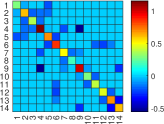
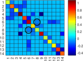
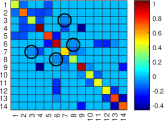
Figure 1: Illustration of the ML-BEST topology recovery methods to estimate the Laplacian matrix of the IEEE-14 bus system with $N=200$ samples and SNR$=15$dB: (a) the original Laplacian matrix; (b) and (c) the estimated Laplacian by two-phase ML-BEST and Augmented Lagrangian ML-BEST methods, respectively. The black circles indicate false connections.

The performance of the different methods is presented in Fig. 2 versus SNR for $N=200$ and $N=1,500$. It can be seen that the performance improves in any sense as $N$ increases, as expected. In Fig 2.a the MSE of the proposed ML-BEST methods for topology estimation and the associated CRB are presented, and in Fig. 2.b the F-score metric of the two ML-BEST methods is presented. It can be seen that while the two-phase topology recovery performs better in terms of F-score, the two ML-BEST methods have similar performance in terms of MSE. That is, the two-phase topology recovery is better in terms of estimating the connectivity matrix, i.e. it distinguishes between existing and absent links, while the performance of both topology recovery methods are close to the CRB for high SNR. However, since the CRB does not take into account the information on inequality constrains [62, 63, 64, 65], and especially the sparsity constraint, it could be slightly higher than the true performance. The MSE of the state estimators presented in Fig. 2.c is similar for the two methods in this case. It can be seen that for high SNRs, the state estimation performance of the ML-BEST methods with estimated topology converges to that of the oracle method, which uses the true topology. Therefore, we can conclude that for high SNRs the topology estimation convergences to the true topology.

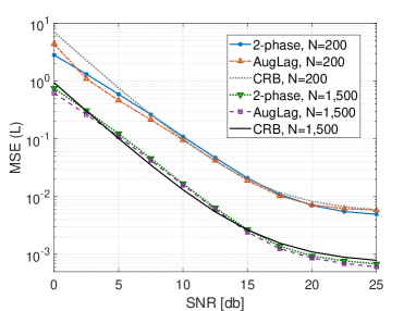
(a) MSE of the topology estimation and the associated CRB

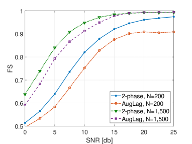
(b) FS

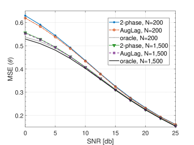
(c) MSE of the state estimators

Figure 2: The performance of the ML-BEST methods, with two-phase and augmented Lagrangian topology recovery, for IEEE-14 bus system versus SNR with $N=200$, $1,500$.

VII-B Random topology

In this subsection we simulate graphs from the Watts-Strogatz ’small world’ graph model [68] with varying numbers of buses, $M$, and an average nodal degree of 4, which is shown to be appropriate for the simulation of synthetic power grid data [43]. It should be noted that the average nodal degree of a power network is almost invariant to the size of the network and, thus, the sparsity level is usually a constant around $\frac{4M}{M^{2}}$. The state covariance matrix set to ${\mbox{\boldmath$\Sigma$}}_{\mbox{\boldmath{\scriptsize$\theta$}}}=c^{2}{\bf{I}}_{M}$, with $c=\sqrt{10}$. In order to achieve uniform SNR simulations, we set the norm of the Laplacian matrix to $||{\bf{L}}||_{F}=5$.

Fig. 3 presents a random graph and its recovery by the ML-BEST methods for $N=200$ and $\sigma^{2}=1$. The red lines in this figure indicate missing connected edges between buses 3 and 5, and buses 5 and 7. This comparison shows that the estimated graphs are generally correspond to the original graph and, thus, the network could be reconstructed by the proposed procedures. The missing recovered edges can be reconstructed by acquiring more data or by setting the sparse threshold more carefully.

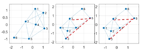
Figure 3: Illustration of the ML-BEST topology recovery methods to estimate the Laplacian matrix of random topology with $N=200$ and $\sigma^{2}=1$: the original graph (left) and the estimated graph topology by two-phase ML-BEST (middle) and Augmented Lagrangian ML-BEST (right). The red lines indicate missing recovered edges.

The performance of the different methods for this random topology is presented in Fig. 4 versus the number of buses in the system for $\sigma^{2}=1$, $N=200,1,500$, and $c=\sqrt{10}$. In Fig 4.a the MSE of the ML-BEST methods for topology estimation and the associated CRB are presented. It can be seen that the topology MSE degraded as $M$ increases since there are more parameters to estimate. The CRB does not take into account the sparsity and, thus, is higher than the true performance. However, it is still a good predictor for the performance, and, thus, can be used for future system design. In Fig. 4.b the F-score metric of the two ML-BEST methods is presented. It can be seen that it is almost independent of the number of buses, $M$, and that the two methods achieve similar results. The MSE of the state estimators presented in Fig. 4.c is lower for the two-phase ML-BEST method with $N=200$, but for $N=1,500$ the Augmented Lagrangian ML-BEST has lower MSE. Thus, different method should be used, depends of the number of samples. The performance of the two methods become closer to those of the oracle performance as $N$ increases. Since the mixing matrix has the same norm for any number of buses, $M$, the SNR is a constant. The structure of the Laplacian matrix leads to a lower MSE of the state estimation as $M$ increases.

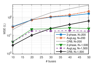
(a) MSE of the topology estimation and the associated CRB

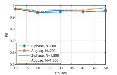
(b) FS

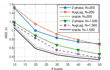
(c) MSE of the state estimators

Figure 4: The performance of the ML-BEST methods, with two-phase and augmented Lagrangian topology recovery, for random topology versus the number of buses with $N=200,1,500$ and for $\sigma^{2}=1$.

In order to demonstrate the empirical complexity of the proposed methods for different problem dimensions, the average computation time, “runtime”, was evaluated by running the algorithm using Matlab on an Intel Core(TM) i7-7600U CPU computer, 2.80 GHz. Figure 5 shows the runtime of the ML-BEST methods as a function of the number of buses, $M$, for a random topology and $N=200,1,500$ samples. It can be seen that the runtime increases polynomially with the number of buses, $M$, and it is higher for the two-phase topology recovery than for the augmented Lagrangian topology recovery with $100$ iterations, as expected from the theoretical discussion on computational complexity in Subsection V-B. The reason for this is that the two-phase topology recovery stage from Algorithm 2 requires solving an SDP problem in (40) and, therefore, has a much higher computational complexity as compared to the augmented ML-BEST estimator. The number of measurements, $N$, has a less significant effect since it is only associated with the cost of computing the sample covariance matrix and the state estimation at the beginning and the end of the basic ML-BEST approach.

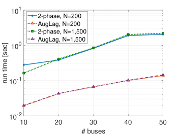
Figure 5: Runtime of the ML-BEST methods versus number of buses, $M$, in random topology with $N=200,1,500$ samples.

VIII Conclusion

In this paper, we introduce the novel ML-BEST method for blind estimation of states and topology in power systems, by formulating the problem as a GBSS with a Laplacian mixing matrix. Since the topology recovery stage of the ML-BEST is shown to be a NP-hard optimization problem, we propose two low-complexity algorithms for the implementation of the topology recovery stage of the ML-BEST estimator: 1) a two-phase topology recovery algorithm, which finds the relaxed positive semidefinite mixing matrix solution and then finds the closest Laplacian matrix to this solution by using convex optimization; 2) an augmented Lagrangian topology recovery algorithm, which is based on classical cICA approaches. These methods rely only on the SOS of the state signals and, in contrast to classical BSS techniques, enable the separation of Gaussian sources. We present some identifiability conditions for this GBSS problem, complexity analysis of the proposed ML-BEST methods, and the associated CRB of the demixing parameters. Numerical simulations show that the proposed ML-BEST methods succeed in reconstructing the topology and estimating the states, and that the topology estimators achieve the CRB asymptotically. The augmented Lagrangian ML-BEST may be preferable for large networks, since the two-phase ML-BEST is a computationally heavy algorithm, as described in Subsection V-B. Additionally, the state estimators converge to the oracle state estimator, which assumes perfect knowledge of the topology.

State estimation is the backbone of power system monitoring and processing. The presented results indicate that even if the topology recovery is not perfect, the MSE of the state estimation is close to the MSE of the oracle performance. Thus, the proposed ML-BEST methods can be applied for practical power system operations without assuming knowledge of the topology. In future work, the proposed methods will be extended to address complex random states, by incorporating concepts from complex BSS [69] and the proposed GBSS approach. For the sparsity pattern, more general thresholding functions should be investigated, as well as theoretical recovery guarantees.

References

- [1] A. Abur and A. Gomez-Exposito, Power System State Estimation: Theory and Implementation. Marcel Dekker, 2004.
- [2] G. B. Giannakis, V. Kekatos, N. Gatsis, S. J. Kim, H. Zhu, and B. F. Wollenberg, “Monitoring and optimization for power grids: A signal processing perspective,” IEEE Signal Processing Magazine, vol. 30, no. 5, pp. 107–128, Sept. 2013.
- [3] Y. Liao, Y. Weng, M. Wu, and R. Rajagopal, “Distribution grid topology reconstruction: An information theoretic approach,” in 2015 North American Power Symposium (NAPS), Oct. 2015, pp. 1–6.
- [4] G. Cavraro and V. Kekatos, “Graph Algorithms for Topology Identification using Power Grid Probing,” ArXiv e-prints, Mar. 2018.
- [5] J. Kim and L. Tong, “On topology attack of a smart grid: Undetectable attacks and countermeasures,” IEEE Journal on Selected Areas in Communications, vol. 31, no. 7, pp. 1294–1305, July 2013.
- [6] S. Cui, Z. Han, S. Kar, T. T. Kim, H. V. Poor, and A. Tajer, “Coordinated data-injection attack and detection in the smart grid: A detailed look at enriching detection solutions,” IEEE Signal Processing Magazine, vol. 29, no. 5, pp. 106–115, Sept. 2012.
- [7] S. Soltan, M. Yannakakis, and G. Zussman, “Power grid state estimation following a joint cyber and physical attack,” IEEE Trans. Control of Network Systems, vol. PP, no. 99, pp. 1–1, 2016.
- [8] T. Routtenberg and Y. C. Eldar, “Centralized identification of imbalances in power networks with synchrophasor data,” IEEE Trans. on Power Systems, vol. 33, no. 2, pp. 1981–1992, 2018.
- [9] T. Routtenberg, Y. Xie, R. M. Willett, and L. Tong, “PMU-based detection of imbalance in three-phase power systems,” IEEE Trans. Power System, vol. 30, no. 4, pp. 1966–1976, July 2015.
- [10] R. Emami and A. Abur, “Tracking changes in the external network model,” in North American Power Symposium 2010, Sep. 2010, pp. 1–6.
- [11] Y. Sharon, A. M. Annaswamy, A. L. Motto, and A. Chakraborty, “Topology identification in distribution network with limited measurements,” in PES Innovative Smart Grid Technologies (ISGT), Jan. 2012, pp. 1–6.
- [12] K. A. Clements and P. W. Davis, “Detection and identification of topology errors in electric power systems,” IEEE Trans. Power Systems, vol. 3, no. 4, pp. 1748–1753, Nov. 1988.
- [13] X. Li, H. V. Poor, and A. Scaglione, “Blind topology identification for power systems,” in IEEE International Conference on Smart Grid Communications (SmartGridComm), Oct. 2013, pp. 91–96.
- [14] A. Anwar, A. Mahmood, and M. Pickering, “Estimation of smart grid topology using SCADA measurements,” in IEEE International Conference on Smart Grid Communications (SmartGridComm), Nov. 2016, pp. 539–544.
- [15] D. Deka, M. Chertkov, and S. Backhaus, “Structure learning in power distribution networks,” IEEE Trans. Control of Network Systems, pp. 1–1, 2018.
- [16] Y. Yuan, O. Ardakanian, S. H. Low, and C. Tomlin, “On the inverse power flow problem,” 2016. [Online]. Available: http://arxiv.org/abs/1610.06631
- [17] S. Bolognani, N. Bof, D. Michelotti, R. Muraro, and L. Schenato, “Identification of power distribution network topology via voltage correlation analysis,” in IEEE Conference on Decision and Control, Dec. 2013, pp. 1659–1664.
- [18] V. Kekatos, G. B. Giannakis, and R. Baldick, “Online energy price matrix factorization for power grid topology tracking,” IEEE Trans. Smart Grid, vol. 7, no. 3, pp. 1239–1248, May 2016.
- [19] S. Xie, J. Yang, K. Xie, Y. Liu, and Z. He, “Low-sparsity unobservable attacks against smart grid: Attack exposure analysis and a data-driven attack scheme,” IEEE Access, vol. 5, pp. 8183–8193, 2017.
- [20] P. Comon, “Independent component analysis, a new concept?” Signal Processing, vol. 36, no. 3, pp. 287–314, Apr. 1994.
- [21] D. T. Pham and P. Garat, “Blind separation of mixture of independent sources through a quasi-maximum likelihood approach,” IEEE Trans. Signal Processing, vol. 45, no. 7, pp. 1712–1725, July 1997.
- [22] A. Belouchrani, K. Abed-Meraim, J. F. Cardoso, and E. Moulines, “A blind source separation technique using second-order statistics,” IEEE Trans. Signal Processing, vol. 45, no. 2, pp. 434–444, Feb. 1997.
- [23] J. F. Cardoso, “Blind signal separation: statistical principles,” Proceedings of the IEEE, vol. 86, no. 10, pp. 2009–2025, Oct. 1998.
- [24] P. Tichavsky, Z. Koldovsky, and E. Oja, “Performance analysis of the FastICA algorithm and Cramr-Rao bounds for linear independent component analysis,” IEEE Trans. Signal Process., vol. 54, no. 4, pp. 1189–1203, Apr. 2006.
- [25] E. Doron, A. Yeredor, and P. Tichavsky, “Cramr Rao-induced bound for blind separation of stationary parametric Gaussian sources,” IEEE Signal Processing Letters, vol. 14, no. 6, pp. 417–420, June 2007.
- [26] A. Yeredor, “Blind separation of Gaussian sources with general covariance structures: Bounds and optimal estimation,” IEEE Trans. Signal Processing, vol. 58, no. 10, pp. 5057–5068, Oct. 2010.
- [27] D. Lahat, J. F. Cardoso, and H. Messer, “Second-order multidimensional ICA: Performance analysis,” IEEE Trans. Signal Process., vol. 60, no. 9, pp. 4598–4610, Sept. 2012.
- [28] T. Routtenberg and J. Tabrikian, “MIMO-AR system identification and blind source separation for GMM-distributed sources,” IEEE Trans. Signal Processing, vol. 57, no. 5, pp. 1717–1730, May 2009.
- [29] ——, “Blind MIMO-AR system identification and source separation with finite-alphabet,” IEEE Trans. Signal Processing, vol. 58, no. 3, pp. 990–1000, Mar. 2010.
- [30] S. Degerine and A. Zaidi, “Separation of an instantaneous mixture of gaussian autoregressive sources by the exact maximum likelihood approach,” IEEE Trans. Signal Processing, vol. 52, no. 6, pp. 1499–1512, June 2004.
- [31] D. T. Pham and J. F. Cardoso, “Blind separation of instantaneous mixtures of nonstationary sources,” IEEE Trans. Signal Processing, vol. 49, no. 9, pp. 1837–1848, Sept. 2001.
- [32] A. Ortega, P. Frossard, J. Kovačević, J. M. F. Moura, and P. Vandergheynst, “Graph signal processing: Overview, challenges, and applications,” Proceedings of the IEEE, vol. 106, no. 5, pp. 808–828, May 2018.
- [33] A. J. Smola and R. Kondor, Kernels and Regularization on Graphs. Berlin, Heidelberg: Springer Berlin Heidelberg, 2003, pp. 144–158.
- [34] S. K. Narang, Y. H. Chao, and A. Ortega, “Graph-wavelet filterbanks for edge-aware image processing,” in 2012 IEEE Statistical Signal Processing Workshop (SSP), Aug. 2012, pp. 141–144.
- [35] M. Newman, Networks: An Introduction. New York, NY, USA: Oxford University Press, Inc., 2010.
- [36] E. Pavez and A. Ortega, “Generalized Laplacian precision matrix estimation for graph signal processing,” in 2016 IEEE International Conference on Acoustics, Speech and Signal Processing (ICASSP), Mar. 2016, pp. 6350–6354.
- [37] H. E. Egilmez, E. Pavez, and A. Ortega, “Graph learning from data under laplacian and structural constraints,” IEEE Journal of Selected Topics in Signal Processing, vol. 11, no. 6, pp. 825–841, Sept 2017.
- [38] D. Ramirez, A. G. Marques, and S. Segarra, “Graph-signal reconstruction and blind deconvolution for diffused sparse inputs,” in 2017 IEEE International Conference on Acoustics, Speech and Signal Processing (ICASSP), Mar. 2017, pp. 4104–4108.
- [39] R. Shafipour, S. Segarra, A. G. Marques, and G. Mateos, “Identifying the Topology of Undirected Networks from Diffused Non-stationary Graph Signals,” ArXiv e-prints, 2018.
- [40] I. Gera, Y. Yakoby, and T. Routtenberg, “Blind estimation of states and topology (BEST) in power systems,” in IEEE Global Conference on Signal and Information Processing (GlobalSIP), Nov. 2017, pp. 1080–1084.
- [41] B. Gustavsen and A. Semlyen, “Enforcing passivity for admittance matrices approximated by rational functions,” IEEE Trans. Power Systems, vol. 16, no. 1, pp. 97–104, Feb. 2001.
- [42] A. Papoulis, Probability, Random Variables, and Stochastic Processes, 3rd ed., 1991.
- [43] Z. Wang, A. Scaglione, and R. J. Thomas, “Generating statistically correct random topologies for testing smart grid communication and control networks,” IEEE Trans. Smart Grid, vol. 1, no. 1, pp. 28–39, June 2010.
- [44] G. Seber, A Matrix Handbook for Statisticians. Hoboken, NJ: Wiley-Interscience, 2008.
- [45] O. Kosut, L. Jia, R. J. Thomas, and L. Tong, “Malicious data attacks on the smart grid,” IEEE Trans. Smart Grid, vol. 2, no. 4, pp. 645–658, Dec 2011.
- [46] R. Gallager, Stochastic Processes: Theory for Applications, ser. Stochastic Processes: Theory for Applications. Cambridge University Press, 2013.
- [47] T. W. Anderson and H. Rubin, “Statistical inference in factor analysis,” 1956.
- [48] L. Tong, R. w. Liu, V. C. Soon, and Y. F. Huang, “Indeterminacy and identifiability of blind identification,” IEEE Trans. Circuits and Systems, vol. 38, no. 5, pp. 499–509, May 1991.
- [49] P. Stoica and M. Jansson, “On maximum likelihood estimation in factor analysis—an algebraic derivation,” Signal Processing, vol. 89, no. 6, pp. 1260–1262, 2009.
- [50] S. M. Kay, Fundamentals of statistical signal processing: Estimation Theory. Englewood Cliffs (N.J.): Prentice Hall PTR, 1993, vol. 1.
- [51] S. Boyd and L. Vandenberghe, Convex Optimization. New York, NY, USA: Cambridge University Press, 2004.
- [52] D. L. Donoho and M. Elad, “Optimally sparse representation in general (non-orthogonal) dictionaries via minimization,” in Proc. of the National Academy of Science USA, vol. 100, no. 5, Mar. 2003, pp. 2197–2202.
- [53] M. A. Davenport, M. F. Duarte, Y. C. Eldar, and G. Kutyniok, “Introduction to compressed sensing,” 2012, compressed Sensing: Theory and Applications, Edited by Y. C. Eldar and G. Kutyniok, Cambridge University Press.
- [54] R. Horn and C. R. Johnson, Matrix Analysis. New York, NY: Cambridge University Press, 1985.
- [55] T. Zhang, A. Wiesel, and M. S. Greco, “Multivariate generalized gaussian distribution: Convexity and graphical models,” IEEE Trans. Signal Processing, vol. 61, no. 16, pp. 4141–4148, Aug. 2013.
- [56] M. Grant and S. Boyd, “CVX: Matlab software for disciplined convex programming, version 2.0,” Aug. 2012. [Online]. Available: http://cvxr.com/cvx
- [57] W. Lu and J. C. Rajapakse, “Approach and applications of constrained ICA,” IEEE Transactions on Neural Networks, vol. 16, no. 1, pp. 203–212, Jan 2005.
- [58] D. P. Bertsekas, Ed., Constrained Optimization and Lagrange Multiplier Methods. New York: Academic Press, 1982.
- [59] W. Lu and J. C. Rajapakse, “ICA with reference,” Neurocomputing, vol. 69, no. 16, pp. 2244–2257, 2006, brain Inspired Cognitive Systems.
- [60] S. Amari, “Natural gradient works efficiently in learning,” Neural Computation, vol. 10, no. 2, pp. 251–276, 1998.
- [61] M. Anderson, G. S. Fu, R. Phlypo, and T. Adali, “Independent vector analysis: Identification conditions and performance bounds,” IEEE Trans. Signal Process., vol. 62, no. 17, pp. 4399–4410, Sept. 2014.
- [62] J. D. Gorman and A. O. Hero, “Lower bounds for parametric estimation with constraints,” IEEE Trans. Inf. Theory, vol. 36, no. 6, pp. 1285–1301, Nov. 1990.
- [63] P. Stoica and B. C. Ng, “On the Cramr-Rao bound under parametric constraints,” IEEE Signal Processing Letters, vol. 5, no. 7, pp. 177–179, July 1998.
- [64] E. Nitzan, T. Routtenberg, and J. Tabrikian, “Cramr-Rao-rao bound for constrained parameter estimation using lehmann-unbiasedness,,” submitted to IEEE Trans. Signal Processing. [Online]. Available: https://arxiv.org/abs/1802.02384
- [65] Z. Ben-Haim and Y. C. Eldar, “The Cramr-Rao bound for estimating a sparse parameter vector,” IEEE Trans. Signal Process., vol. 58, no. 6, pp. 3384–3389, June 2010.
- [66] “Power systems test case archive.” [Online]. Available: http://www.ee.washington.edu/research/pstca/
- [67] H. E. Egilmez, E. Pavez, and A. Ortega, “Graph learning from data under structural and Laplacian constraints,” IEEE Journal of Selected Topics in Signal Processing, vol. 11, no. 6, pp. 825–841, Sept. 2017.
- [68] “Collective dynamics of small-world networks,” Nature, pp. 393–440, 1998.
- [69] T. Adali, P. J. Schreier, and L. L. Scharf, “Complex-valued signal processing: The proper way to deal with impropriety,” IEEE Trans. Signal Processing, vol. 59, no. 11, pp. 5101–5125, Nov. 2011.