On the Reconstruction of Static and Dynamic Discrete Structures

Abstract.

We study inverse problems of reconstructing static and dynamic discrete structures from tomographic data (with a special focus on the ‘classical’ task of reconstructing finite point sets in $\mathbb{R}^{d}$). The main emphasis is on recent mathematical developments and new applications, which emerge in scientific areas such as physics and materials science, but also in inner mathematical fields such as number theory, optimization, and imaging. Along with a concise introduction to the field of discrete tomography, we give pointers to related aspects of computerized tomography in order to contrast the worlds of continuous and discrete inverse problems.

1. Introduction

We begin with an informal definition of the general field of discrete tomography. As a comprehensive treatise of the general field would, however, go far beyond the scope of the present paper, and as we want to limit the overlap with surveys in the literature as much as possible, we will focus on the most fundamental case of reconstructing finite point sets in $\mathbb{R}^{d}$ from some of their discrete X-rays. Our special emphasis will be on (a subjective selection of) recent developments and applications. We conclude the introduction with a few comments on the structure of the paper and its bibliography.

1.1. What is discrete tomography?

Discrete tomography deals with the problem of retrieving knowledge about an otherwise unknown discrete object from information about its interactions with certain query sets. Of course, this is not a formal definition and, as a matter of fact, the occuring terms leave room for different interpretations. For instance, the discrete object can be any set in some $\mathbb{R}^{d}$ that allows a finite encoding, e.g., a finite point set, a polytope or even a semialgebraic set. Also functions with finite support are included. Knowledge may mean full reconstruction, the detection of certain properties and measures of the object or just a ‘yes/no’ decision whether the object equals (or is close to) a given blueprint. The query sets may be windows, affine spaces or certain families of more general manifolds, and interaction may simply mean intersection but could also refer to a very different probing procedure.

While results which, in retrospective, belong to this area go back a long time, the name discrete tomography and the establishment of the so-named field is of more recent origin. In the past decades the focus has been on the issues of uniqueness, computational complexity, and algorithms, first under the theoretical assumption that exact X-ray data were available. Later, stability and instability questions were pursued, and the effect of noise was studied.

Discrete tomography has important applications in physics, materials science, and many other fields. It has, however, also been applied in various other contexts, including scheduling [101], data security [112], image processing [127], data compression [126], combinatorics [53, 81, 92, 95], and graph theory [89, 90]. Closely connected are also several recreational games such as nonograms [75], path puzzles [78], sudokus [87], and color pic-a-pix [70].

1.2. Scope of the present paper

In the following we will concentrate mainly on the ‘classical’ task of reconstructing a finite point set in $\mathbb{R}^{d}$ from the cardinalities of its intersections with the lines parallel to a (small) finite number of directions. Already in this restricted form, discrete tomography displays important features also known from the continuous world. In particular, discrete tomography is ill-posed in the sense of Hadamard [29]: the data may be inconsistent, the solution need not be unique (Thm. 1), and small changes in the data may result in dramatic changes of the solutions (Thm. 12).

As will become clear, discrete tomography is not simply the discretization of continuous tomography. It derives its special characteristics from the facts that, on the one hand, there are only data in very few directions available, but on the other hand, the classes of objects that have to be reconstructed are rather restricted. Therefore discrete tomography is based on methods from combinatorics, discrete optimization, algebra, number theory, and other more discrete subfields of mathematics and computer science.

There exist already books and articles, which give detailed accounts of various aspects of discrete tomography and its applications. We single out [21, 25, 26, 28, 36, 37, 52]. The present article differs from these surveys in various ways: the mathematical focus will be on recent developments (which have not been covered in previous surveys). Further, new applications will play a significant role, i.e., applications to other scientific areas like physics and materials science, but also to inner mathematical fields such as number theory, optimization, and imaging. We will, moreover, include pointers to certain related aspects of computerized tomography in order to contrast the worlds of continuous and discrete inverse problems. As general sources for the continuous case and inverse problems, see [33, 42, 44, 45] and [7, 31, 39, 43, 58], respectively.

As a service to the reader and with a view towards a more complete picture we will restate some aspects which are basic for the present article but have been covered before. In order to limit the overlap to other surveys we will, however, neither elude on the tomographic reconstruction of quasicrystals (see [25]) or polyominoes (see [18]), nor on the polyatomic case (see [22, 94]) or point X-rays (see [91]). Also, we will not study general $k$-dimensional X-rays (see [25, 103]) but concentrate on the case $k=1$. This means that our exposition will be based on the X-ray transform rather than on the Radon transform (which is the case $k=d-1)$.

1.3. Organization of the present paper and its bibliography

After introducing the basic notation in Sect. 2 we will briefly survey well-known structural results related to the ill-posedness of the problems (Sect. 3) and their computational complexity (Sect. 4). Turning to recent results and applications, Sect. 5 will illustrate some quite unexpected complexity jumps in (a related basic model of) superresolution. Particular emphasis will then be placed on new developments in dynamic discrete tomography involving the movement of points over time which are only accessible by very few of their X-ray images. As Sect. 6 will show aspects of discrete tomography and particle tracking interact deeply. Another more recent issue, which comes up in materials science, is that of multi-scale tomographic imaging. Sect. 7 will indicate how different aspects of the reconstruction of polycrystalline materials based on tomographic data lead to very different techniques involving methods from the geometry of numbers, combinatorial optimization and computational geometry. Sect. 8 deals with some inner mathematical connections between discrete tomography and the Prouhet-Tarry-Escott problem from number theory, and Sect. 9 concludes with some final remarks.

Let us point out that (with the exception of some new interpretations and simple observations) the results stated here have all been published in original research papers (which are, of course, cited appropriately). Even more, since we want to use the standard notation and, in particular, a standard framework for expressing the results, some overlap with the above mentioned surveys is unavoidable.

Finally, let us close the introcuction with a comment on the bibliography. Due to the character of the present paper we included references of different kinds. Of course, we listed all original work quoted in the main body of the paper. However, we felt that for the generally interested reader it would be worthwhile to add sources for general reading. On the other hand, in terms of the included applications we focussed mainly on outlining those aspects to which discrete tomography can potentially contribute. While this is in line with the scope of the present paper, readers interested in these fields of applications may appreciate pointers to sources for additional reading. Hence we organized the bibliography in six different parts, namely general reading, papers in tomography, and further reading on particle tracking, tomographic grain mapping, macroscopic grain mapping, and the Prouhet-Tarry-Escott problem, respectively.

2. Basic notation

As pointed out before we will focus on the ‘classical’ inverse problem of reconstructing a finite point set $F$ in $\mathbb{R}^{d}$ or $\mathbb{Z}^{d}$ from the cardinalities of its intersections with the lines parallel to a finite number of directions. There are, however, certain aspects which involve weights on the points of $F$. Hence we will introduce the basic notions for appropriate generalizations of characteristic functions of finite point sets, partly following [25].

As usual, let $\mathbb{N}_{0}$, $\mathbb{N}$, $\mathbb{Z},$ $\mathbb{Q},$ and $\mathbb{R}$ denote the sets of non-negative integers, natural numbers, integers, rationals, and reals, respectively. Further, for $n\in\mathbb{N},$ we will often use the notation $[n]=\{1,\dots,n\}$ and $[n]_{0}=[n]\cup\{0\}$.

In the following, let $d,m\in\mathbb{N}$; $d$ denotes the dimension of the space $\mathbb{R}^{d}$, and $m$ is the number of directions in which images are taken. To exclude trivial cases, we will usually assume that $d,m\geq 2$.

In oder to describe the objects of interest, we fix nonempty sets $D\subset\mathbb{R}^{d}$ and $C\subset\mathbb{R}$ and consider functions $\psi\!:\,D\rightarrow C$ with finite support $\textnormal{supp}(\psi)=\{x\in D:\psi(x)\neq 0\}$. In our context, the most relevant pairs $(D,C)$ of a domain and a codomain are those where $D=\mathbb{R}^{d}$ or $D=\mathbb{Z}^{d}$ and $C=\{0,1\}$. Other standard codomains are $C=\mathbb{N}_{0}$, $C=\mathbb{Z},$ and also their relaxations $[0,1]$, $[0,\infty[$, and $\mathbb{R}$.

For any pair $(D,C)$, let $\mathcal{F}(D,C)$ denote the class of all functions $\psi\!:\,D\rightarrow C$ with finite support. Of course, for $C=\{0,1\}$, such a function $\psi$ can be viewed as the indicator or characteristic function of a finite set $F$ and can therefore be identified with $\textnormal{supp}(\psi)$. We will write $\mathcal{F}(D)$ for $\mathcal{F}(D,\{0,1\})$ and identify it with the set of all finite subsets of $D$. In particular, the case $\mathcal{F}(\mathbb{Z}^{d})$ encodes the classical finite lattice sets. Since this case is particularly important we will often abbreviate $\mathcal{F}(\mathbb{Z}^{d})$ by $\mathcal{F}^{d}$.

Further, let $\mathcal{S}^{d}$ denote the set of all $1$-dimensional subspaces of $\mathbb{R}^{d}$, while $\mathcal{L}^{d}$ is the set of $1$-dimensional lattice lines, i.e., lines through the origin spanned by an integer vector. For $S\in\mathcal{S}^{d}$, we use the notation ${\mathcal{A}}(S)$ for the set of all affine lines in $\mathbb{R}^{d}$ that are parallel to $S$. The situation of $(\mathcal{F}^{d},\mathcal{L}^{d})$ will be referred to as the lattice case.

Now, let $\psi\in\mathcal{F}(D,C)$ and $S\in\mathcal{S}^{d}$. The discrete X-ray of $\psi$ parallel to $S$ (or, in a slight abuse of language, in the direction $S$) is the function $X_{S}\psi\!:\,\mathcal{A}(S)\rightarrow\mathbb{R}$ defined by

$$T\,\longmapsto\,\bigl{(}X_{S}\psi\bigr{)}(T)\,=\sum_{x\in T}\psi(x).$$

Since $\psi$ has finite support all sums are finite. In the case of $C=\{0,1\}$ where $\psi$ can be identified with $F=\textnormal{supp}(\psi)$, we will often write $X_{S}F$. See Fig. 1 for an illustration.

Figure 1. A finite lattice set (black dots) and its 1-dimensional X-rays in the two directions $(1,1)^{T}$ and $(1,-2)^{T}.$

The mapping $\mathcal{X}_{\psi}$ on $\mathcal{S}^{d}$ defined by $S\mapsto X_{S}\psi$ is called the discrete X-ray transform of $\psi$. (In typical applications only very few values of $\mathcal{X}_{\psi}$ are available.)

Note that it is straightforward to extend this notation to $k$-dimensional X-rays. Accordingly, for $k=d-1$, we obtain the discrete Radon transform of $\psi$ whose measurements come from hyperplane X-rays. We will, however, focus on the X-rays defined above, which provide $1$-dimensional measurements. The basic task of discrete tomography is then to reconstruct an otherwise unknown function $\psi\in\mathcal{F}(D,C)$ from its X-rays with respect to a finite number $m$ of given lines $S\in\mathcal{S}^{d}$.

The X-ray information is encoded by means of data functions. In fact, the lines $T\in{\mathcal{A}}(S)$ can be parametrized by vectors $t\in S^{\perp}$ such that $T=t+S$. Hence, one may regard $X_{S}\psi$ as a function on $S^{\perp}$. For algorithmic purposes, it is often preferable to use other representations and encode $X_{S}\psi$ as a finite set of pairs $(x,\beta)$ with $x\in D$, $\beta\in C$ and $X_{S}\psi(x+S)=\beta$.

3. Ill-posedness

We begin with some results that deal with the basic issues of uniqueness and stability.

3.1. Uniqueness and non-uniqueness

Given a subset $\mathcal{F}$ of $\mathcal{F}(D)$, and $\mathcal{S}\subset\mathcal{S}^{d}$. We say that two different sets $F_{1},F_{2}\in\mathcal{F}$ are tomographically equivalent with respect to $\mathcal{S}$ if $X_{S}F_{1}=X_{S}F_{2}$ for all $S\in\mathcal{S}$. The pair $(F_{1},F_{2})$ will then also be referred to as a switching component. Further, a set $F\in\mathcal{F}$ is uniquely determined within $\mathcal{F}$ by its X-rays parallel to the lines in $\mathcal{S}$ if there does not exist any other set $F^{\prime}$ in $\mathcal{F}$ that is tomographically equivalent to $F$ with respect to $\mathcal{S}$. If the context is clear we will simply say that $F\in\mathcal{F}$ is uniquely determined.

The following classical non-uniqueness result, usually attributed to [120], has been rediscovered several times.

Theorem 1.

For any finite subset $\mathcal{L}$ of $\mathcal{L}^{d}$ there exist sets in $\mathcal{F}^{d}$ that cannot be determined by $X$-rays parallel to the lines in $\mathcal{L}.$

Figure 2 gives an illustration of the typical construction process to obtain different lattice sets with equal X-rays.

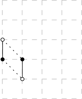
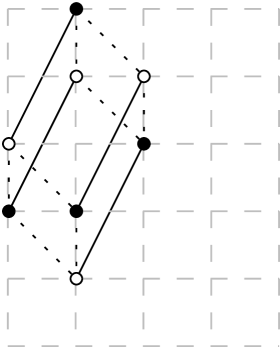
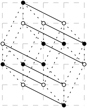
Figure 2. Construction of different lattice sets (black and white points) with equal X-rays in (a) two, (b) three, and (c) four directions.

Note that Thm. 1 is in accordance with similar results in continuous or geometric tomography. In fact, let $\mathcal{S}\subset\mathcal{S}^{d}$ be finite, and let $C,K\in\mathbb{R}^{d}$ be compact and $C\subset{\mathrm{int}}(K)$. Further let $f:\mathbb{R}^{d}\rightarrow\mathbb{R}$ be infinitely often differentiable with support $K$. Then there is a function $g$ with support in $K$, infinitely often differentiable, but otherwise arbitrary on $C$ such that the continuous X-rays of $f$ and $g$ with respect to all lines in $\mathcal{S}$ coincide; for a proof, see [128]. Also, characteristic functions of compact sets, i.e., functions $f:\mathbb{R}^{d}\to\{0,1\}$ with compact support are not determined by their (continuous) X-rays in any finite number of directions; see [21, Thm. 2.3.3].

While non-uniqueness is an undesirable feature for many applications it will play a positive role for applications in number theory later; see Sect. 8.

In contrast to Thm. 1, uniqueness of the reconstruction can sometimes be guaranteed when certain prior knowledge is available.

Theorem 2.

There exists a line $S\in\mathcal{S}^{d}$ such that every set $F\in\mathcal{F}^{d}$ is uniquely determined by its one X-ray $X_{S}F$.

At first glance, this result may seem surprising. However, the used a priori information is that the set is contained in $\mathbb{Z}^{d}$. Then, indeed, the X-ray $X_{S}F$ for any one line in $\mathcal{S}^{d}\setminus\mathcal{L}^{d}$ determines $F$ uniquely, simply because no translate of $S$ can contain more than one lattice point. As this argument shows, Thm. 2 can easily be extended to $\mathcal{F}(\mathbb{Z}^{d},C).$

While Thm. 2 does not seem to be of great practical use, it shows nonetheless that no matter how fine the lattice discretization might be, one X-ray suffices. In the limit, however, finitely many X-rays do in general not suffice. In this sense, discrete tomography does not behave like a discretization of continuous tomography. Note that Thm. 2 is quite different in nature from a result of [128] (see also [42, Thm. 3.148]) that for almost any finite dimensional space of objects its elements can be distinguished by a single X-ray in almost any direction. In fact, $\mathcal{F}^{d}$ is not finite-dimensional, and moreover, any line $S\in\mathcal{S}^{d}\setminus\mathcal{L}^{d}$ works for any set $F\in\mathcal{F}^{d},$ i.e., $S$ does not depend on the set but is given beforehand.

The next result is due to Rényi [123] for $d=2$, who attributes an algorithmic proof to Hajós. The generalization to $d\geq 2$ was given by Heppes [108].

Theorem 3 ([123] Rényi).

Let $\mathcal{S}$ be a finite subset of $\mathcal{S}^{d}$. Then every set $F\in\mathcal{F}(\mathbb{R}^{d})$ with $|F|\leq|\mathcal{S}|-1$ is uniquely determined by its X-rays parallel to the lines in $\mathcal{S}$.

Since the two color classes of the two-coloring of the vertices of the regular $2m$-gon in the plane are tomographically equivalent with repect to the lines parallel to its edges, Thm. 3 is best possible. A strengthening for (mildly) restricted sets of directions is given in [77]. But even more: generic directions are much better.

Theorem 4 ([122]).

There exist constants $c>0$ and $m_{0}\in\mathbb{N}$ such that for all $m\geq m_{0}$ the following holds: For almost all sets $\mathcal{S}\subset\mathcal{S}^{2}$ of $m$ directions any $F\in\mathcal{F}(\mathbb{R}^{2})$ with $|F|\leq 2^{cm/\log(m)}$ is uniquely determined by its X-rays parallel to the lines of $\mathcal{S}$.

Let us point out that in continuous tomography it is well-known that a compactly supported, infinitely differentiable function $f:\mathbb{R}^{d}\to\mathbb{R},$ which does not contain ‘details of size $2\pi/b$’ or smaller can be recovered reliably from its X-rays on special sets of $m$ directions, provided that $m>b.$ For a precise statement and proof, see [44, Thm. 2.4]. See also [41]. Such a result can be viewed, to some extent, as an analogue to Rényi’s theorem. (Note, however, that the difference to $f$ is measured in an integral norm and hence the difference may get arbitrarily small without ever reaching $0$. For a characterization of the null-space, see [41, 121].)

For the special case $m=|\mathcal{S}|=2,$ uniqueness within $\mathcal{F}^{2}$ is characterized by the work of Ryser [52]. See Fig. 3 for an example of a set of $12$ points in $\mathbb{Z}^{2}$ that is uniquely determined by its two X-rays in the coordinate directions. For uniqueness results from two directions in geometric tomography, see [118, 120].

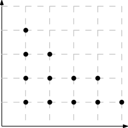
Figure 3. A lattice set (black points) uniquely determined by its X-rays in horizontal and vertical directions.

In the lattice case, the specialization of Rényi’s theorem that any set $F\in\mathcal{F}^{d}$ is determined by any set of $|F|+1$ lattice lines is only best possible for the cardinalities $|F|=m\in\{1,2,3,4,6\}$. For other $m$ the result can be improved at least by $1$.

Theorem 5 ([69]).

Let $m\in\mathbb{N}\setminus\{1,2,3,4,6\}$ and let $\mathcal{F}^{d}(m)$ be the class of sets in $\mathcal{F}^{d}$ of cardinality less than or equal to $m.$ Let $\mathcal{L}\subset\mathcal{L}^{d}$ with $|\mathcal{L}|\geq m.$ Then the sets in $\mathcal{F}^{d}(m)$ are determined by their X-rays parallel to the lines in $\mathcal{L}.$

The question of smallest switching components is widely open in the lattice case.

Problem 1.

What is the smallest number $n=n(d,m)$ such that there exist $\mathcal{L}\subset\mathcal{L}^{d}$ with $|\mathcal{L}|=m$ and two different lattice sets $F_{1},F_{2}\in\mathcal{F}^{d}$ of cardinality $n$ that are tomographically equivalent with respect to the lines in $\mathcal{L}$?

Probabilistic arguments of [69] show that, in the lattice case, switching components of a size that is polynomial in $m$ exist for each $d$. All deterministic constructions so far lead to exponential size switching components. Several small switching components are depicted in Fig. 12.

We remark that switching components seem to have appeared first in the work of Ryser [52]. Later work on switching components includes [38, 86, 107, 117, 122, 125]. Computational investigations related to the explicit construction of switching components can be found in [82]. Switching components for other projection models are considered in [129, 130, 131, 132, 138]. Special types of switching components in the context of superresolution imaging, $hv$-convex polynomioes, and, in a more algebraic setting, are studied in [67], [73], and [117], respectively.

Quite strong uniqueness results exist for a geometrically motivated more restricted class of lattice sets. A lattice set $F\in\mathcal{F}^{d}$ is called convex, if

$$F={\mathrm{conv}}(F)\cap\mathbb{Z}^{d}.$$

Theorem 6 ([98]).

There are $S_{1},S_{2},S_{3},S_{4}\in\mathcal{L}^{d}$ such that every finite convex lattice set $F$ is uniquely determined by $X_{S_{1}}F,\ldots,X_{S_{4}}F$. Further, every set of at least seven coplanar lattice lines always suffices.

Let us point out that the ‘good’ sets of directions with respect to Thm. 6 need not have coordinates of large absolute value. Examples for $d=2$ are

$$\{(1,0)^{T},(1,1)^{T},(1,2)^{T},(1,5)^{T}\}\quad\textnormal{and}\quad\{(1,0)^{T},(2,1)^{T},(0,1)^{T},(-1,2)^{T}\}.$$

In fact, the sets of four good lattice lines in Thm. 6 are those whose cross-ratio of their slopes does not lie in $\{4/3,3/2,2,3,4\}$. A converse result for the more general class of hv-convex lattice sets is given in [72]. Generalizations of Thm. 6 to so-called Q-convex lattice sets and convex algebraic Delone sets (in the context of quasicrystals) can be found in [88] and [111], respectively.

As a matter of fact, the directions in Thm. 6 are all coplanar. It is not known how exactly the situation changes if we insist that the lines are in general position, i.e., each $d$ of them span $\mathbb{R}^{d}.$

Problem 2.

Let $d\geq 3$. Is there a finite subset $\mathcal{L}$ of lines in $\mathcal{L}^{d}$ in general position such that each convex set in $\mathcal{F}^{d}$ is uniquely determined by its X-rays parallel to the lines in $\mathcal{L}?$ If so, what is the smallest cardinality?

Is there a smallest number $m$ such that any set $\mathcal{L}\subset\mathcal{L}^{d}$ of $m$ lines has the property, that each convex set in $\mathcal{F}^{d}$ is uniquely determined by its X-rays parallel to the lines in $\mathcal{L}$?

The color classes of a $2$-coloring of the vertices of the permutahedron in $\mathbb{R}^{d}$ provide a lower bound on such a universal number, which grows at least quadratically in $m$ [63]. Fig. 4 depicts the $3$-dimensional permutahedron, which is a truncated octahedron.

Figure 4. Two-coloring of the vertices of the truncated octahedron.

An analogue to Thm. 6 also holds in the realm of geometric tomography: convex subsets of $\mathbb{R}^{d}$ are determined by their continuous X-rays from sets of four ‘good’ directions, see [102].

Let us point out that it is the codomain $\{0,1\}$ which makes the problem difficult. In fact, the case of functions in $\mathcal{F}(\mathbb{Z}^{d},\mathbb{Z})$ or, equivalently, lattice sets with integer weights is much simpler, as linear diophantine equations can be solved via the Hermite normal form; see e.g. [54, Sect. 4&5]). But this also implies that the study of uniqueness for functions $\psi\in\mathcal{F}(\mathbb{Z}^{d},\mathbb{N}_{0})$ is much easier. In fact, suppose we are given a finite set $\mathcal{L}\subset\mathcal{L}^{d}$ and a bounded subset $B$ of $\mathbb{Z}^{d}$ which will act as a superset of all supports we are allowing. Then the corresponding X-ray problem with data functions all identical to $0$ can be formulated as a homogenous system of linear diophantine equations and solved efficiently. Let $\psi$ be a non trivial solution, define $\psi^{+}:\mathbb{Z}^{d}\to\mathbb{R}$ by

$$\psi^{+}(x)=\begin{cases}\psi(x)&\mbox{if $\psi(x)>0$;}\\ 0&\mbox{if $\psi(x)\leq 0$;}\end{cases}$$

for $x\in\mathbb{Z}^{d}$, and set

$$\psi^{-}=\psi^{+}-\psi.$$

Then, of course, $\psi^{+},\psi^{-}\in\mathcal{F}(\mathbb{Z}^{d},\mathbb{N}_{0})$, $\psi=\psi^{+}-\psi^{-}$, and $X_{S}\psi\equiv 0$ for all $S\in\mathcal{L}$. Hence, $\psi^{+},\psi^{-}$ are tomographically equivalent with respect to $\mathcal{L}$.

The uniqueness problem for functions $\psi\in\mathcal{F}(\mathbb{Z}^{d},\mathbb{N}_{0})$ also permits an algebraic characterization. The subsequently stated result of Hajdu and Tijdeman [30, 107] uses the following notation. A vector $v=(\nu_{1},\dots,\nu_{d})^{T}\in\mathbb{Z}^{d}$ is reduced if $\textnormal{gcd}(\nu_{1},\dots,\nu_{d})=1.$ Let $v^{+}$ and $v^{-}$ denote the vectors whose $j$th component is $\nu_{j}^{+}=\max\{0,\nu_{j}\}$ and $\nu_{j}^{-}=\max\{0,-\nu_{j}\},$ respectively. With $\boldsymbol{X}$ we abbreviate the vector $(X_{1},\dots,X_{d})$ of indeterminants. Accordingly, for $a=(\alpha_{1},\dots,\alpha_{d})^{T}\in\mathbb{N}_{0}^{d}$, the monomial $X_{1}^{\alpha_{1}}\cdot\ldots\cdot X_{d}^{\alpha_{d}}\in\mathbb{Z}[\boldsymbol{X}]$ is denoted by $\boldsymbol{X}^{a}$.

Theorem 7 ([30, 107]).

Let $\psi,\varphi\in\mathcal{F}(\mathbb{N}_{0}^{d},\mathbb{N}_{0}),$ let $v\in\mathbb{Z}^{d}$ be reduced, and set $S={\mathrm{lin}}\{v\}$. Then $X_{S}\psi=X_{S}\varphi$ if, and only if, the polynomial

$$\sum_{a\in\textnormal{supp}(\psi)}\boldsymbol{X}^{a}-\sum_{b\in\textnormal{supp}(\varphi)}\boldsymbol{X}^{b}$$

is divisible by $\boldsymbol{X}^{v+}-\boldsymbol{X}^{v^{-}}.$

Note that the assumption that the functions are defined on $\mathbb{N}_{0}^{d}$ rather than on $\mathbb{Z}^{d}$ is no restriction of generality.

Let $v^{(1)},\dots,v^{(m)}\in\mathbb{Z}^{d}\setminus\{0\}$ be reduced, $\mathcal{S}=\{{\mathrm{lin}}\{v^{(1)}\},\dots,{\mathrm{lin}}\{v^{(m)}\}\}$ and

$$f_{\mathcal{S}}=\prod_{v\in\{v^{(1)},\dots,v^{(m)}\}}(\boldsymbol{X}^{v^{+}}-\boldsymbol{X}^{v^{-}}).$$

A consequence of Thm. 7 is that $\psi,\varphi\in\mathcal{F}(\mathbb{N}_{0}^{d},\mathbb{N}_{0})$ are tomographically equivalent with respect to $\mathcal{S}$ if, and only if, there is a polynomial $p$ in $\mathbb{Z}[\boldsymbol{X}]$ such that

$$\sum_{a\in\textnormal{supp}(\psi)}\boldsymbol{X}^{a}-\sum_{b\in\textnormal{supp}(\varphi)}\boldsymbol{X}^{b}=p\cdot f_{\mathcal{S}}.$$

The algebraic representation by polynomials can be utilized in various ways; examples will be given in Sect. 3.2 (stability) and 8 (number theory). Additional aspects of uniqueness, in particular, concepts of additivity, are discussed in [60, 95, 104]. For uniqueness results for functions in $\mathcal{F}(\mathbb{N}_{0}^{d},\{0,1\})$ with several different types of bounded support, see [83] and the references cited therein.

3.2. Stability and instability

The results of the previous section were based on the assumption that the data functions are given exactly. We will now consider the case that the X-rays may contain errors.

In the following we will measure the size of a function $\psi\in\mathcal{F}(D,C)$ in terms of its $\ell_{1}$-norm, i.e.,

$$\|\psi\|_{1}=\sum_{x\in D}|\psi(x)|.$$

In particular, given a finite set $\mathcal{S}\subset\mathcal{S}^{d}$ of lines and two sets $F_{1},F_{2}\in\mathcal{F}(\mathbb{R}^{d})$ their X-ray difference will be

$$\Delta_{\mathcal{S}}(F_{1},F_{2})=\sum_{S\in\mathcal{S}}||X_{S}F_{1}-X_{S}F_{2}||_{1}.$$

The first result in this section shows that at least some (however marginal) stability is present. In fact, the X-ray difference, if not $0$, must jump to at least $2(m-1)$. This means that either two sets are tomographically equivalent or their X-ray difference grows at least linearly in $m$.

Theorem 8 ([64]).

Let $\mathcal{S}\subset\mathcal{S}^{d}$, $|\mathcal{S}|=m$, and $F_{1},F_{2}\in\mathcal{F}(\mathbb{R}^{d})$ with $|F_{1}|=|F_{2}|$. If $\Delta_{\mathcal{S}}(F_{1},F_{2})<2(m-1)$, then $F_{1}$ and $F_{2}$ are tomographically equivalent with respect to $\mathcal{S}$. The same statement holds in the lattice case.

As we will see in Thm. 12, this result is, in fact, best possible. First, we use it to give ‘noisy’ variants of some of the uniqueness results of the previous section. We begin with a stable version of Thm. 3.

Theorem 9 ([64]).

Let $\mathcal{S}\subset\mathcal{S}^{d}$, $F_{1},F_{2}\in\mathcal{F}(\mathbb{R}^{d})$, and $\Delta_{\mathcal{S}}(F_{1},F_{2})<2|F_{1}|$. Further, let $|F_{1}|=|F_{2}|$ and $|F_{1}|+1\leq|\mathcal{S}|$, or let $|F_{1}|\leq|F_{2}|$ and $2|F_{1}|\leq|\mathcal{S}|$. Then $F_{1}=F_{2}$. The statement persists in the lattice case.

The following result is a stable version of Thm. 6.

Theorem 10 ([64]).

There are sets $\mathcal{S}\subset\mathcal{L}^{d}$ of cardinality $4$ for which the following is true: If $F_{1},F_{2}\in\mathcal{F}^{d}$ are convex, and $|F_{1}|=|F_{2}|$, but $F_{1}\neq F_{2}$, then $\Delta_{\mathcal{S}}(F_{1},F_{2})\geq 6$. Further, for any set $\mathcal{S}\subset\mathcal{L}^{d}$ of at least $7$ coplanar lattice lines, and sets $F_{1},F_{2}$ as before, $\Delta_{\mathcal{S}}(F_{1},F_{2})\geq 2(|\mathcal{S}|-1)$.

The following theorem uses the known characterization of the (rather rare) cases of uniqueness in the special case $d=m=2$ to quantify the deviation of solutions for noisy data; it generalizes a previous result from [61].

Theorem 11 ([135]).

Let $\mathcal{S}\subset\mathcal{L}^{2}$ with $|\mathcal{S}|=2$, let $F_{1},F_{2}\in\mathcal{F}^{2}$ with $|F_{1}|=|F_{2}|$. Further, suppose that $F_{1}$ is uniquely determined by $X_{S}F_{1}$ for $S\in\mathcal{S}$, and set $\beta=\Delta_{\mathcal{S}}(F_{1},F_{2})$. Then

$$4|F_{1}\cap F_{2}|+(\beta+2)\Bigl{(}\beta-1+\sqrt{8|F_{1}\cap F_{2}|+(\beta-1)^{2}}\Bigr{)}\geq 4|F_{1}|.$$

Stability results in the continuous case with finitely many X-rays typically rely on bounds of the variation of the functions, measured in some weighted Sobolev norms; see [44, Sect. 4] and [42, Sect. 5.9] (and references therein). In the realm of geometric tomography, Volčič [136] showed that the problem of reconstructing a convex body from its X-rays in four ‘good’ directions (which guarantee uniqueness) is well-posed. Some further stability estimates are given in [119].

In contrast to Thm. 11, the task of reconstructing finite lattice sets from X-rays taken along $m\geq 3$ directions is highly instable. In particular the following result shows that Thm. 8 is sharp.

Theorem 12 ([3, 68]).

Let $\mathcal{S}\subset\mathcal{S}^{d}$ with $|\mathcal{S}|\geq 3$, and let $\alpha\in\mathbb{N}$. Then there exist $F_{1},F_{2}\in\mathcal{F}(\mathbb{R}^{d})$ with the following properties:

1. $F_{1}$ is uniquely determined by $X_{S}F_{1}$ for $S\in\mathcal{S}$;

2. $F_{2}$ is uniquely determined by $X_{S}F_{2}$ for $S\in\mathcal{S}$;

3. $\Delta_{\mathcal{S}}(F_{1},F_{2})=2(m-1)$;

4. $|F_{1}|=|F_{2}|\geq\alpha$;

5. $F_{1}\cap F_{2}=\emptyset$.

The statement also holds in the lattice case.

The proof for $d=2$ is due to [68], while [3] extends the construction to general $d$. It is actually possible to show that not even affine transformations help much to increase the overlap of the two sets.

4. Computational aspects

Next we deal with algorithmic aspects of actually reconstructing the, one or all sets that are consistent with the given X-ray data. We will restrict the exposition to functions in $\mathcal{F}(\mathbb{Z}^{d},C)$ with $C\subset\mathbb{Q}$ and lines in $\mathcal{L}^{d}$ since all computational issues can then be studied in the well-known binary Turing machine model; see [23, 47] for background information. Again, emphasis will be placed on the lattice case.

4.1. Algorithmic problems

Let $\mathcal{S}\subset\mathcal{L}^{d}$ be finite. From an algorithmic point of view the following questions are basic: Are the data consistent? If so, reconstruct a solution! Is this solution unique? We will now introduce the correponding problems more precisely.

Consistency${}_{\mathcal{F}(\mathbb{Z}^{d},C)}(\mathcal{S})$.

• Data functions $f_{S}$ for $S\in\mathcal{S}$.

• Does there exist $\psi\in\mathcal{F}(\mathbb{Z}^{d},C)$ such that $X_{S}\psi=f_{S}$ for all $S\in\mathcal{S}$?

Reconstruction${}_{\mathcal{F}(\mathbb{Z}^{d},C)}(\mathcal{S})$.

• Data functions $f_{S}$ for $S\in\mathcal{S}$.

• Determine a function $\psi\in\mathcal{F}(\mathbb{Z}^{d},C)$ such that $X_{S}\psi=f_{S}$ for all $S\in\mathcal{S}$, or decide that no such function exists.

Uniqueness${}_{\mathcal{F}(\mathbb{Z}^{d},C)}(\mathcal{S})$.

• A function $\psi\in\mathcal{F}(\mathbb{Z}^{d},C)$.

• Does there exist $\varphi\in\mathcal{F}(\mathbb{Z}^{d},C)\setminus\{\psi\}$ such that $X_{S}\psi=X_{S}\varphi$ for all $S\in\mathcal{S}$?

Of course, Reconstruction${}_{\mathcal{F}(\mathbb{Z}^{d},C)}(\mathcal{S})$ cannot be easier than Consistency${}_{\mathcal{F}(\mathbb{Z}^{d},C)}(\mathcal{S})$. Further, note that Uniqueness${}_{\mathcal{F}(\mathbb{Z}^{d},C)}(\mathcal{S})$ actually asks for nonuniqueness in order to place the problem into the class $\mathbb{N}\mathbb{P}$; see Thm. 13.

For certain codomains such as $C=\{0,1\}$ it is reasonable to actually ask for the number of solutions even in the case of non-uniqueness. We will introduce the following problem for geneneral $C$ with the understanding that the (not really interesting) answer ‘$\infty$’ is permitted.

$\#$Consistency${}_{\mathcal{F}(\mathbb{Z}^{d},C)}(\mathcal{S})$.

• Data functions $f_{S}$ for $S\in\mathcal{S}$.

• Determine the cardinality of the set of functions $\psi\in\mathcal{F}(\mathbb{Z}^{d},C)$ such that $X_{S}\psi=f_{S}$ for all $S\in\mathcal{S}$.

Observe that a given instance $\mathcal{I}=(f_{S}:S\in\mathcal{S})$ can be consistent only if $\|f_{S}\|_{1}$ does not depend on $S$. Since this condition can be checked efficiently we will in the following often tacitly assume that this is the case and set

$$n=n({\mathcal{I}})=\|f_{S}\|_{1}.$$

Further, for any given instance $\mathcal{I}=(f_{S}:S\in\mathcal{S})$, the support of all solutions is contained in the grid

$$G\,=\,G({\mathcal{I}})\,=\,\bigcap_{S\in\mathcal{S}}\bigl{(}\textnormal{supp}(f_{S})+S\bigr{)}$$

associated with $\mathcal{I}$. Of course, $G({\mathcal{I}})$ can be computed from $\mathcal{I}$ by solving polynomially many systems of linear equations. Hence we can associate a variable $x_{g}$ with every grid point and formulate Consistency${}_{\mathcal{F}(\mathbb{Z}^{d},C)}(\mathcal{S})$ as a linear (feasibility) problem with the additional constraints that $x_{g}\in C$ for all $g\in G$. This simple observation shows already that Consistency${}_{\mathcal{F}(\mathbb{Z}^{d},C)}(\mathcal{S})$ is algorithmically easy for $C\in\{[0,1]\cap\mathbb{Q},\mathbb{Q}\}$ simply because linear programming can be solved in polynomial time, and also for $C=\mathbb{Z}$ since systems of linear diophantine equations can be solved in polynomial time; see e.g. [54, Sect. 4,5,13–15].

Next we are turning to the other relevant codomains, with a special emphasis on the lattice case.

Theorem 13 ([52, 96, 100]).

Consistency${}_{\mathcal{F}(\mathbb{Z}^{d},C)}(\mathcal{S})$ and Uniqueness${}_{\mathcal{F}(\mathbb{Z}^{d},C)}(\mathcal{S}),$ $C\in\{\{0,1\},\mathbb{N}_{0}\},$ are both in $\mathbb{P}$ if $|\mathcal{S}|\leq 2$ whereas they are $\mathbb{N}\mathbb{P}$-complete if $|\mathcal{S}|\geq 3.$ Also, the problem $\#$Consistency${}_{\mathcal{F}^{d}}(\mathcal{S})$ is $\#\mathbb{N}\mathbb{P}$-complete for $|\mathcal{S}|\geq 3$.

The complexity status of the counting problem for $|\mathcal{S}|=2$ is still open.

Problem 3.

Is $\#$Consistency${}_{\mathcal{F}^{d}}(\mathcal{S}),$ $|\mathcal{S}|=2,$ a $\#\mathbb{P}$-complete problem?

Let us now return to the Rényi setting.

Theorem 14 ([108, 123]).

Reconstruction${}_{\mathcal{F}^{d}}(\mathcal{S})$ is in $\mathbb{P}$ if the input is restricted to those instances $\mathcal{I}=(f_{S}:S\in\mathcal{S})$ with $n(\mathcal{I})<|\mathcal{S}|.$

A similar result holds for convex lattice sets when the lattice lines are chose according to Thm. 6. So, let $\mathcal{C}^{d}$ denote the subset of $\mathcal{F}^{d}$ of convex lattice set, and let Reconstruction${}_{\mathcal{C}^{d}}(\mathcal{S})$ signify the correponding reconstruction task.

Theorem 15 ([79, 80]).

For any set $\mathcal{S}\subset\mathcal{L}^{d}$ of at least seven coplanar directions and for suitable such sets of cardinality four Reconstruction${}_{\mathcal{C}^{d}}(\mathcal{S})$ can be solved in polynomial-time.

Let us now turn to the following ‘noisy’ versions of Consistency${}_{\mathcal{F}^{d}}(\mathcal{S})$ and Uniqueness${}_{\mathcal{F}^{d}}(\mathcal{S}).$

X-Ray-Correction${}_{\mathcal{F}^{d}}(\mathcal{S})$.

• Data functions $f_{S}$ for $S\in\mathcal{S}.$

• Does there exist $F\in\mathcal{F}^{d}$ such that
  $\displaystyle\sum_{S\in\mathcal{S}}||X_{S}F-f_{S}||_{1}\leq m-1?$

Similar-Solution${}_{\mathcal{F}^{d}}(\mathcal{S})$.

• A set $F_{1}\in\mathcal{F}^{d}.$

• Does there exist $F_{2}\in\mathcal{F}^{d}$ with $|F_{1}|=|F_{2}|$ and $F_{1}\neq F_{2}$ such that $\Delta_{\mathcal{S}}(F_{1},F_{2})\leq 2m-3?$

Nearest-Solution${}_{\mathcal{F}^{d}}(\mathcal{S})$.

• Data functions $f_{S}$ for $S\in\mathcal{S}.$

• Determine a set $F^{*}\in\mathcal{F}^{d}$ such that
  $\displaystyle\sum_{S\in\mathcal{S}}||X_{S}F^{*}-f_{S}||_{1}=\min_{F\in\mathcal{F}^{d}}\sum_{S\in\mathcal{S}}||X_{S}F-f_{S}||_{1}.$

Note that X-Ray-Correction${}_{\mathcal{F}^{d}}(\mathcal{S})$ can also be viewed as the task of deciding, for given data functions $f_{S},$ $S\in\mathcal{S},$ whether there exist ‘corrected’ data functions $f^{\prime}_{S},$ $S\in\mathcal{S},$ that are consistent and do not differ from the given functions by more than a total of $m-1$. Nearest-Solution${}_{\mathcal{F}^{d}}(\mathcal{S})$ asks for a set $F^{*}\in\mathcal{F}^{d}$ that fits the potentially noisy measurements best.

The computational complexity of these tasks is as follows.

Theorem 16 ([64]).

The problems X-Ray-Correction${}_{\mathcal{F}^{d}}(\mathcal{S})$, Similar-Solution${}_{\mathcal{F}^{d}}(\mathcal{S})$, and Nearest-Solution${}_{\mathcal{F}^{d}}(\mathcal{S})$ are in $\mathbb{P}$ for $|\mathcal{S}|\leq 2$ but are $\mathbb{N}\mathbb{P}$-complete for $|\mathcal{S}|\geq 3.$

4.2. Algorithms

Several polynomial-time algorithms for Reconstruction${}_{\mathcal{F}(\mathbb{Z}^{d},C)}(\mathcal{S}),$ $C\in\{\{0,1\},\mathbb{N}_{0}\},$ $|\mathcal{S}|=2,$ can be found in the literature. In addition to Ryser’s algorithm [52] for $C=\{0,1\},$ there are approaches based on network-flows [127] or matroid intersections [99]. Moreover, the problem can be modeled as an integer linear program, which involves a totally unimodular coefficient matrix, and which can therefore be solved as a linear program (see, for instance, [54, Sect. 16&19]). For further comments, see [36, Sect. 1].

In the presence of $\mathbb{N}\mathbb{P}$-hardness, one cannot expect to find generally efficient algorithms. There are, however, various techniques from combinatorial optimization that can and have been applied to solve instances to optimality up to certain sizes; see [105]. Similarly as for $|\mathcal{S}|=2,$ the reconstruction problem Reconstruction${}_{\mathcal{F}(\mathbb{Z}^{d},C)}(\mathcal{S}),$ $C\in\{\{0,1\},\mathbb{N}_{0}\},$ can be formulated als integer linear program for arbitrary $|\mathcal{S}|.$ However, for $|\mathcal{S}|\geq 3$ the coefficient matrix is in general no longer totally unimodular. Of course, we can still solve the corresponding linear programming relaxation (where $\{0,1\}$ is replaced by $[0,1]$ or $\mathbb{N}_{0}$ by $[0,\infty[$) efficiently. Unless $\mathbb{P}=\mathbb{N}\mathbb{P},$ Thm. 13 implies that it will, however, in general not be efficiently possible to convert the obtained fractional solution into a required integer one.

Since, in general, measured data are noisy anyway, research focused on approximate solutions. It is quite natural to try to solve Reconstruction${}_{\mathcal{F}^{d}}(\mathcal{S})$ even if $|\mathcal{S}|\geq 3$ by using the available polynomial-time algorithms for $|\mathcal{S}|=2$ in an alternating approach. First, two of the given $|\mathcal{S}|$ data functions are selected and a solution $F_{0}$ is computed which is consistent with these. In the $j$th step, at least one of the two directions is replaced by a different one from $\mathcal{S},$ and a solution is constructed which satisfies the corresponding two constraints and is closest to $F_{j}$. While each step of such an alternating direction approach can be performed in polynomial time, there are severe limitations on the guaranteed quality of the produced solution. For an analysis of this and other approaches, see [105].

Despite their theoretical limitations there are several approaches that are reported to work very well in practice. Among these are BART [109] and DART [76, 137]. The former, which is a variant of ART as described in [34], is implemented in the open-source software SNARK14 [116] (example code can be found in [62]), the latter is implemented in the open-source ASTRA toolbox [133]. Further algorithms are discussed in [36, Sect. 8-14] and [37, Sect. 8-11]. For applets illustrating several algorithmic tasks in discrete and geometric tomography, see [93] and [97], respectively.

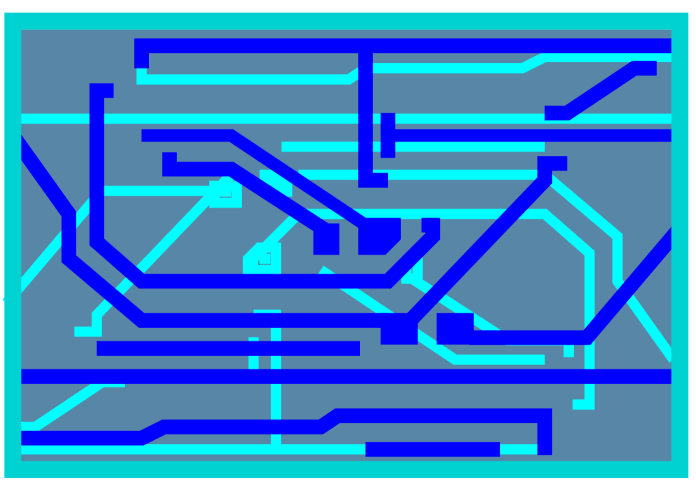
Figure 5. (From [27]) An idealized circuit board.

Let us, finally, point out that for certain applications full reconstructions are not needed. For instance, in quality control for circuit board productions (see Fig. 5) one may want to certify that the production process actually produced a desired blueprint structure (‘verification’). Then one can, of course, compute data functions from the blueprint and compare them with the measured data from the produced board. If the difference is large one would report an error. If, however, the difference is small, the produced board can still be quite different from the blueprint (particularly if the data do not determine the image uniquely). This ambiguity can be reduced by applying a (polynomial-time deterministic) reconstruction heuristic on both sets of data functions and subsequently comparing the reconstructions. In practice such checks have shown to be able to detect production flaws even on very limited data and quite poor (and very fast) reconstructions algorithms.

5. Superresolution and discrete tomography

Electron tomography, pioneered originally in the life sciences (see [20, 35, 46]), is becoming an increasingly important tool in materials science for studying the three-dimensional morphologies and chemical compositions of nanostructures [62, 71, 74, 114]. For various technical reasons, however, atomic resolution tomographic imaging as envision in [115, 124] has not become a full reality yet (favorable instances are reported in [113, 134]; see also the surveys [10, 56]). One of the challenges faced by current technology is that tomographic tilt series need to be properly aligned (see, e.g., [57, 110]). Therefore, and also to prevent radiation damage, one might wonder whether is is possible to proceed in a multimodal scheme.

Suppose some reconstruction has been obtained from a (possibly technologically less-demanding) lower-resolution data set. Can one then use limited additional high-resolution data (for instance, acquired from only two directions) to enhance the resolution in a subsequent step? As we will now see the tractability of this approach depends strongly on the reliability of the initial lower-resolution reconstruction. Details of the presented results can be found in [67].

5.1. Computational aspects

We have already remarked that a function $\psi\in\mathcal{F}^{d}$ can be viewed as a characteristic function that encodes a finite lattice set. In a different, yet equivalent, model the function $\psi$ can be viewed as representing a binary image. In this interpretation the points $x\in\mathbb{Z}^{d}$ represent the pixel/voxel coordinates while $\psi(x)$ denotes their colors (typically, values 0 and 1 are considered to represent white and black pixels, respectively); see Fig. 6 for an illustration. Similarly, for $l\in\mathbb{N},$ a function $\rho\in\mathcal{F}(\mathbb{Z}^{d},[l]_{0})$ can be viewed as representing a gray-scale image with $l+1$ different gray levels (values $0$ and $l$ typically representing the ‘gray level’ white and black, respectively).

Figure 6. Lattice points (left) and pixels (middle); right: pixel associated with its lattice point.

For simplicity of the exposition we restrict our discussion to the case $d=2$. Now suppose we want to reconstruct a binary image $\psi\in\mathcal{F}^{2}$ contained in an $n_{1}\times n_{2}$ box from low-resolution gray scale information and high-resolution X-ray data. The lower resolution is quantified by some $k\in\mathbb{N}\setminus\{1\}$, and we assume that $n_{1}$ and $n_{2}$ are divisible by $k$. More precisely, we assume that an $n_{1}/k\times n_{2}/k$ low-resolution (gray-scale) image $\rho\in\mathcal{F}(\mathbb{Z}^{2},[k^{2}]_{0})$ of $\psi$ is available, and the pixels $x$ in $\psi$ result from a $k\times k$ subdivision of the pixels $y$ of $\rho.$ Hence in any such subdivision $B$ we have

$$\sum_{x\in B}\psi(x)=\rho(y).$$

For given $\rho(y)$ and unknown $\psi(x),$ $x\in B,$ we call the above equation a $k\times k$ block constraint. We say that, for some $\varepsilon\in\mathbb{N}_{0}$, a block constraint is satisfied within an error of $\varepsilon$, if

$$\rho(y)-\varepsilon\>\>\leq\>\>\sum_{x\in B}\psi(x)\>\>\leq\>\>\rho(y)+\varepsilon.$$

We may think of $\rho$ as being the result of some lower-resolution reconstruction of $\psi$. In order to increase the resolution we want to utilize additional high-resolution X-ray data $X_{S}\psi$ that are available from the two coordinate directions $S_{1}$ and $S_{2}$, and we set $\mathcal{S}=\{S_{1},S_{2}\}$. Relatively to $\rho$ the data $X_{S}\psi,$ $S\in\mathcal{S}$, can be considered as $k$-times finer resolution X-ray data.

For given $k\geq 2$ and $\varepsilon\in\mathbb{N}_{0}$ the task of (noisy) superresolution is as follows.

nSR$(k,\varepsilon)$.

• A gray-level image $\rho\in\mathcal{F}(\mathbb{Z}^{2},[k^{2}]_{0}),$
  a subset $R$ of ‘reliable pixels’ of $\rho,$ and
  data functions $f_{S_{1}},f_{S_{2}}$ at a $k$-times finer resolution.

• Determine a function $\psi\in\mathcal{F}^{2}$ such that
  $X_{S}\psi=f_{S}$ for $S\in\{S_{1},S_{2}\},$ all $k\times k$ block constraints for the pixels in $R$ are satisfied, and all other $k\times k$ block constraints are satisfied within an error of $\varepsilon,$
  or decide that no such function exists.

Since our focus is in the following on double-resolution imaging, i.e., on the case $k=2,$ let us set $\textsc{nDR}(\varepsilon)=\textsc{nSR}(2,\varepsilon),$ for $\varepsilon>0.$ In the reliable situation, i.e., for $\varepsilon=0$ we simply speak of double-resolution and set $\textsc{DR}=\textsc{nSR}(2,0).$ (Then, of course, the set $R$ can be omitted from the input.) An illustration is given in Fig. 7.

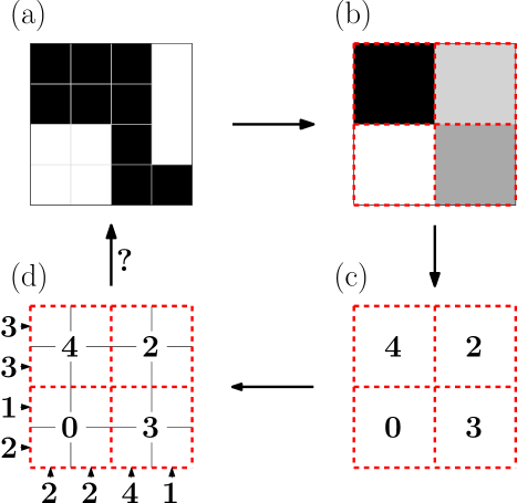
Figure 7. (From [67]) The double-resolution imaging task DR. (a) Original (unknown) high-resolution image, (b) the corresponding low-resolution gray-scale image, (c) gray levels converted into block constraints, (d) taken in combination with double-resolution row and column sum data. The task is to reconstruct from (d) the original binary image shown in (a).

As it turns out DR is tractable.

Theorem 17 ([67]).

DR and also the corresponding uniqueness problem can be solved in polynomial time.

The algorithm presented in [67] is based on a decomposition into subproblems, which allows to treat the different gray levels separately. If we view DR as the reconstruction problem for $m=|\mathcal{S}|=2$ with additionally block constraints we can compare Thm. 17 with Thm. 13 and see that bock constraints impose fewer algorithmic difficulties than X-ray data from a third direction.

The next result, which deals with the case that some of the gray levels come with small uncertainties depicts (potentially unexpected) complexity jumps.

Theorem 18 ([67]).

Let $k\geq 2$ and $\varepsilon>0.$

1. nSR$(k,\varepsilon)$ is $\mathbb{N}\mathbb{P}$-hard.

2. The problem of deciding whether a given solution of an instance of nSR$(k,\varepsilon)$ has a non-unique solution is $\mathbb{N}\mathbb{P}$-complete.

To put it succinctly: noise in tomographic superresolution imaging does not only affect the quality of a reconstructed image but also the algorithmic tractability of the inverse problem itself.

DR without any block constraints boils down to the reconstruction problem for $m=2$ and is hence solvable in polynomial-time. DR is, however, $\mathbb{N}\mathbb{P}$-hard if several (but not all) block constraints (which are required to be satisfied with equality) are present (Thm. 18). Possibly less expectedly, if all block constraints are included, then the problem becomes polynomial-time solvable again (Thm. 17). If, on the other hand, from all block constraints some of the data come with noise at most $1,$ then the problem becomes again $\mathbb{N}\mathbb{P}$-hard (Thm. 18). And yet again, if from all block constraints all of the data are sufficiently noisy, then the problem is in $\mathbb{P}$ (as this is again the problem of reconstructing binary images from X-ray data taken from two directions). Figure 8 gives an overview of these complexity jumps.

Figure 8. (From [67]) Overview of complexity jumps for the problem of reconstructing a binary image from row and column sums and additional $2\times 2$ block constraints.

It does not seem likely that, but is still open, whether the tractability result of Thm. 17 persists for $k\geq 3$.

Problem 4 ([67]).

Is the problem nSR$(k,0)$ $\mathbb{N}\mathbb{P}$-hard for $k\geq 3$?

In the realm of dynamic discrete tomography (see Sect. 6) block constraints play the role of special window constraints which can be used to encoding velocity information for moving points.

For additional information on discrete tomography problems involving other kinds of constraints, see [15, Sect. 4].

5.2. Stability and instability

Let us now turn to a discussion of the stability of the solutions to DR.

Theorem 19.

Let $\mathcal{S}=\{\textnormal{lin}(1,0)^{T},\textnormal{lin}(0,1)^{T}\},$ and $\alpha\in\mathbb{N}$. Then there exist instances $\mathcal{I}_{1}$ and $\mathcal{I}_{2}$ of DR with the following properties:

1. $F_{1}$ is the unique solution to $\mathcal{I}_{1};$

2. $F_{2}$ is the unique solution to $\mathcal{I}_{2};$

3. $\Delta_{\mathcal{S}}(F_{1},F_{2})=4;$

4. $|F_{1}|=|F_{2}|\geq\alpha$;

5. $|F_{1}\cap F_{2}|=\frac{1}{2}|F_{1}|.$

The proof is based on a construction in [67] of an instance $\mathcal{I}$ of DR that admits precisely two solutions $F^{\prime}_{1}\neq F^{\prime}_{2}$ with $|F^{\prime}_{1}|=|F^{\prime}_{2}|\geq\alpha+2.$ From these two solutions points in one block are deleted to obtain $F_{1}$ and $F_{2}$; see Fig. 9 for an illustration.

A small X-ray error of $4$ can thus lead to quite different reconstructions (again, see Fig. 9). It should be noted, however, that the set $F_{2}$ has a much larger total variation (TV) than $F_{1}$ (for some background information see, e.g., [85]). Regularization by total variation minimization, as proposed in [67], would therefore always favor the reconstruction $F_{1}.$

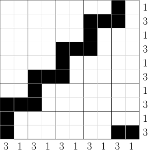
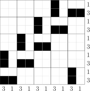
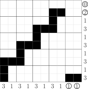
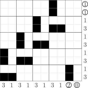
Figure 9. An example illustrating instability of DR. (a) and (b): two solutions of the same problem instance; (c) and (d): uniquely determined solutions $F_{1},$ $F_{2}$ to the two problem instances obtained by deleting points of a block from (a) and (b), respectively. (The X-rays are indicated by the numbers to the bottom and right.) The X-rays differ in the circled numbers yielding an X-ray error $\Delta_{\mathcal{S}}(F_{1},F_{2})=4.$

It is instructive to compare DR (Thm. 19) with its discrete tomography counterparts for $m=2$ (Thm. 11) and $m\geq 3$ (Thm. 12), which do not involve any block constraints.

On the one hand, the reconstruction problem for $m=2$ is much more stable than its double-resolution counterpart. In fact, an easy calculation for $\beta=4$ shows that Thm. 11 implies the bound

$$|F_{1}\cap F_{2}|\geq|F_{1}|-5\sqrt{|F_{1}|}-9.$$

Thus, if the original set $F_{1}$ is uniquely determined by its X-rays, then any reconstruction $F_{2}$ from X-rays with error $4$ needs to coincide with $F_{1}$ by an asymptotically much larger fraction than the $|F_{1}|/2$ provided in Thm. 19 for DR.

On the other hand, the instability result for $m=3$ (see Thm. 12) is stronger than that of Thm. 19 as for the former an X-ray error of 4 can lead to disjoint reconstructions.

Hence in terms of (in-)stabilities the block constraints seem to play a somewhat weaker role than constraints modeling data from a third direction.

6. Dynamics

Let us now turn to dynamic discrete tomography, which, in fact, represents rather recent developments in the field (see [65, 66, 141, 151]). (For dynamic aspects of computerized tomography, see, e.g., [84, 106] and the references cited therein.)

We focus here on the task of tomographic particle (or point) tracking, which amounts to determining the paths $\mathcal{P}_{1},\ldots,\mathcal{P}_{n}$ of $n$ points in space over a period of $t\in\mathbb{N}$ moments in time from X-ray images taken from a fixed number $m$ of directions.

This problem comprises, in fact, two different but coupled basic underlying tasks, the reconstruction of a finite set of points from few of their X-ray images (discrete tomography) and the identification of the points over time (tracking). The latter is closely related to topics in combinatorial optimization including matching and $k$-assigment problems; see [16] for a comprehensive survey on assignment problems.

Let us remark that particle tracking methods have been proven useful in many different fields such as fluid mechanics, geoscience, elementary particle physics, plasma physics, combustion, and biomedical imaging [140, 144, 146, 147, 149, 151] (see also the monograph [2] and the references cited therein). Most previous tomographic particle tracking methods (such as [142, 143, 145, 150]) can be considered as particle imaging velocimetry (PIV) as they aim at capturing several statistical parameters of groups of particles instead of dealing with them individually. The individual tracking considered here is in the literature also sometimes referred to as particle tracking velocimetry (PTV) or low particle number density PIV [140]. For more general background information on particle tracking methods, see the monographs [2, 55].

The exposition in this section will partly follow [66].

6.1. Algorithmic problems

We want to focus here on the interplay between discrete tomography and tracking. Therefore, we will distinguish the cases that for none, some or all of the $\tau\in[t]$ moments in time, a solution $F^{(\tau)}\in\mathcal{F}^{d}$ of the discrete tomography task at time $\tau$ is explicitly available (and is then considered the correct solution regardless whether it is uniquely determined by its X-rays). The former case will be referred to as the (partially) or (totally) tomographic case while we speak of the latter as positionally determined. It should be noted that the positionally determined case can be viewed as being the generic case in $\mathbb{R}^{d},$ $d\geq 3,$ because there any two (affine) lines in general position are disjoint, hence X-ray lines meet only in the points of $F^{(\tau)}.$

For simplicity we assume in the following that there are no particles disappearing or reappearing within the tracked time interval. When $P=\{p_{1},\dots,p_{n}\}$ denotes the (abstract) set of $n$ particles, we are in the tracking step thus interested in a one-to-one mapping $\pi^{(\tau)}:P\to F^{(\tau)},$ $\tau\in[t],$ that identifies the points of $F^{(\tau)}$ with the particles. The particle tracks are then given by $\mathcal{P}_{i}=(\pi^{(1)}(p_{i}),\dots,\pi^{(t)}(p_{i})),$ $i\in[n].$ This identification is referred to as coupling.

In typical applications we would like to incorporate prior knowledge about ‘physically likely’ paths. It seems most natural to input such information in terms of the cost $c(\mathcal{P}_{1},\ldots,\mathcal{P}_{n})$ of the feasible particle tracks. Note, however, that the number of different particle tracks $(\mathcal{P}_{1},\ldots,\mathcal{P}_{n})$ is $(n!)^{t}$, hence exponential in $n$ and $t.$ This means that already for moderate problem sizes the costs of all potential tracks cannot be encoded explicitly. There are various ways to deal with this problem. The most general approach is based on the assumption that ‘an expert knows a good solution if she or he sees it.’ More technically speaking, it is enough for an algorithm to have access to the cost $c(\mathcal{P}_{1},\ldots,\mathcal{P}_{n})$ only when the particle track $c(\mathcal{P}_{1},\ldots,\mathcal{P}_{n})$ is considered. Accordingly, [66] suggest an oracular model, where such knowledge is available through an algorithm $\mathcal{O}$, called an objective function oracle, which computes for any solution $(\mathcal{P}_{1},\ldots,\mathcal{P}_{n})$ its cost $c(\mathcal{P}_{1},\ldots,\mathcal{P}_{n})$ in time that is polynomial in all the other input data. Then the general problem of tomographic particle tracking for $\mathcal{S}\subset\mathcal{S}^{d},$ can be formulated as follows.

TomTrac${(\mathcal{O};\mathcal{S})}$.

• $t\in\mathbb{N}$ and data functions $f^{(\tau)}_{S}$ with $\|f^{(\tau)}_{S}\|_{1}=n,$ for $S\in\mathcal{S},$ $\tau\in[t].$

• Decide whether, for each $\tau\in[t]$, there exists a set $F^{(\tau)}\in\mathcal{F}^{d}$ such that $X_{S}F^{(\tau)}=f_{S}^{(\tau)}$ for all $S\in\mathcal{S}.$ If so, find particle tracks $\mathcal{P}_{1},\ldots,\mathcal{P}_{n}$ of minimal cost for $\mathcal{O}$ among all couplings of all tomographic solutions $F^{(1)},\ldots,F^{(t)}.$

In the positionally determined case the problem TomTrac${(\mathcal{O};\mathcal{S})}$ reduces to the following tracking problem, which can be viewed as a $t$-dimensional assignment problem.

Trac$(\mathcal{O};d)$.

• $t\in\mathbb{N}$ and sets $F^{(1)},\ldots,F^{(t)}\in\mathcal{F}^{d}$ with $|F^{(1)}|=\ldots=|F^{(t)}|=n$.

• Find particle tracks $\mathcal{P}_{1},\ldots,\mathcal{P}_{n}$ of minimal cost for $\mathcal{O}$ among all couplings of the sets $F^{(1)},\ldots,F^{(t)}.$

A priori knowledge may be available in various ways and may then lead to different objective function oracles; see [66]. Here we focus on information that is actually explicitly available. For instance, we speak of a path value oracle if the cost $c(\mathcal{P}_{1},\ldots,\mathcal{P}_{n})$ is just the sum $\sum_{i=1}^{n}w(\mathcal{P}_{i})$ of the weights of the individual paths $\mathcal{P}_{i},$ $i\in[n]$. Note that the number of different weights is bounded by $n^{t}$, and can hence be encoded explicitly for fixed (and small) $t$; see Thm. 22. If, further, the weights are just the sums of all costs of assigning points between consecutive moments in time the objective function can be described by just $(t-1)n^{2}$, i.e., polynomially many numbers. In this case, the objective function is of Markov-type as it reflects only memoryless dependencies. Combinatorial models, which can be viewed as special choices of such parameters, are based on the knowledge that the positions of the particles in the next time step lie in certain windows. A particular such situation has be analyzed in Sect. 5. For more results on combinatorial models see [65, 66].

6.2. Algorithms and complexity

We begin with a simple tractability result for the positionally determined case.

Theorem 20 ([66]).

For Markov-type objective function oracles $\mathcal{O}$ the problem Trac$(\mathcal{O};d)$ decomposes into uncoupled minimum weight perfect bipartite matching problems and can hence be solved in polynomial time.

Although the reconstruction problem in discrete tomography for $|\mathcal{S}|=2$ directions can be solved in polynomial time (see Thm. 13) it turns out that there are severe limitations of extending the previous result already for the following quite restricted partially tomographic case. In fact, the problem becomes hard even if there is only one time step, i.e., $t=2$, and $F^{(1)}$ is explicitly known while the set $F^{(2)}$ of particle positions for $\tau=2$ is only accessible through its two X-rays $X_{S_{1}}F^{(2)}$ and $X_{S_{2}}F^{(2)}$.

Theorem 21 ([66]).

Even if all instances are restricted to the case $t=2$, where the solution $F^{(1)}$ is given explicitly, TomTrac${(\mathcal{O};\mathcal{S})},$ $|\mathcal{S}|=2,$ for Markov-type objective function oracles $\mathcal{O}$ is $\mathbb{N}\mathbb{P}$-hard. Also the corresponding uniqueness problem is $\mathbb{N}\mathbb{P}$-complete and the counting problem is $\#\mathbb{P}$-complete.

Unless $\mathbb{P}=\mathbb{N}\mathbb{P},$ there is thus, in general, no efficient algorithm that provides exact solutions to every instance of TomTrac${(\mathcal{O};\mathcal{S})},$ $|\mathcal{S}|=2.$ A possible remedy is to resort to heuristics, which aim at providing approximate solutions. Before we discuss such a heuristic let us state two additional intractability results, which concern the positionally determined case for non Markov-type function oracles.

Theorem 22 ([66]).

The problem Trac$(\mathcal{O};d)$ is $\mathbb{N}\mathbb{P}$-hard, even if all instances are restricted to a fixed $t\geq 3,$ and $\mathcal{O}$ is a path value oracle. The $\mathbb{N}\mathbb{P}$-hardness persists if the objective function values provided by $\mathcal{O}$ are all encoded explicitly.

It turns out that even if the particles are expected to move along straight lines, this a priori knowledge cannot be exploited efficiently (unless $\mathbb{P}=\mathbb{N}\mathbb{P}$).

Theorem 23 ([66]).

For every fixed $d\geq 2$ and $t\geq 3$ it is an $\mathbb{N}\mathbb{P}$-complete problem to decide whether a solution of Trac$(\mathcal{O};d)$ exists where all particles move along straight lines.

The proof of Thm. 23 given in [66] relies on the hardness of the particular variant A3ap of $3$D-Matching established in [148]. For further results and a discussion of their practical implications see [66].

The previous complexity results show that even for $t=3$ and even if there is no tomography involved the coupling becomes hard unless it is of the Markov-type, i.e., it only incorporates information that relate not more than two consecutive moments in time (Thm. 22). But even for $t=2$, which, of course, is of Markov-type, the problem is hard if tomography is involved at one point in time (Thm. 21). This means that there is not much room for efficient algorithms or ‘self-suggesting’ polynomial-time heuristics.

There are, however, quite involved heuristics for TomTrac${(\mathcal{O};S_{1},S_{2})},$ which allow to incorporate varous different forms of a priori knowledge and different levels of ‘particle history’; see [66]. Here we focus only on one basic method, called Rolling Horizon Tomography, which was introduced in  [141] and applied to the study of the slip velocity of a gliding arc discharge in [151].

The general idea in Rolling Horizon Tomography is to model the time step from $\tau$ to $\tau+1$ as a linear program, based on the assumption that $F^{(1)}$ is known (hence we are dealing with the partially tomographic case). The constraints encode the X-rays provided by the data functions $f_{1}^{(\tau+1)}$, $f_{2}^{(\tau+1)}$. The variables correspond to the points in the grid $G^{(\tau+1)}$ and are collected in a vector $x^{(\tau+1)}$. The X-ray information is encoded by means of a totally unimodular matrix $A^{(\tau+1)}$ and a right-hand side vector $b^{(\tau+1)}$. Further, each point $g_{i}^{(\tau+1)}\in G^{(\tau+1)}$ carries a weight $\alpha_{i}^{(\tau+1)},$ which reflects the ‘distance’ to a best point $g_{i}^{(\tau)}\in F^{(\tau)}$ (which is a likely ‘predecessor’). These weights are collect in a vector $a^{(\tau+1)}$. Various choices of weights are discussed in [141], which, for instance, model knowledge on the velocity of the particles. The algorithm can then be described as follows.

Beginning with $F^{(1)},$ Rolling Horizon Tomography solves successively for $\tau\in[t-1]$ the linear program

$$\begin{array}[]{lrcl}&\lx@intercol\hfil\min\,\,\bigl{(}a^{(\tau+1)}\bigr{)}^{T}x^{(\tau+1)}\hfil\lx@intercol\\[2.84544pt] \textnormal{s.\,t. }&A^{(\tau+1)}x^{(\tau+1)}&=&b^{(\tau+1)},\\ &x^{(\tau+1)}&\leq&1\kern-4.10004pt1,\\ &x^{(\tau+1)}&\geq&0,\\ \end{array}$$

in order to determine $F^{(\tau+1)}$ (via its encoding as a $0$-$1$ incidence vector of a basic feasible solution of the linear program). Finally the paths $\mathcal{P}_{1},\ldots,\mathcal{P}_{n}$ are obtained by a routine that computes a perfect bipartite matching in the graph with vertices $F^{(\tau)}\cup F^{(\tau+1)}$ and edges corresponding to the pairs of vertices that realize the distances $\alpha_{i}^{(\tau)}.$

Rolling Horizon Tomography runs in polynomial time, is exact in the sense that it is guaranteed to return a solution which matches the data. It also allows to incorporate physical knowledge and it is reported to work quite well in practice (see [141, 151]). However, (and with a view to Thm. 21 not surprisingly), it is only a heuristic, which may fail to reconstruct the correct paths. The reason is that the weights used to measure the quality of the assignment do not incorporate the requirement that no two particles can have originated from the same location at the previous moment in time. Explicit example are given in [66] which also gives generalizations that combine the general rolling horizon approach with interpolation and backtracking techniques to provide algorithms that incorporate physical knowledge even better while still running in polynomial time.

7. Tomographic grain mapping

Tomographic grain mapping deals with the problem of characterizing polycrystalline materials from tomographic data. Polycrystalline materials consist of multiple crystals, called grains. These grains, often $10-100$ micrometer in diameter, are of central interest in many areas of materials science as most metals, ceramics and alloys are such polycrystalline materials. In fact, the grains determine many of the material’s physical, chemical, and mechanical properties (see, e.g., [158, 164, 166, 170] or the monographs [40, 51]).

7.1. Diffraction and indexing

There are several non-trivial technological and algorithmical challenges involved in tomographic grain mapping on different scales. Typically, only high-energy X-rays will penetrate the material. In fact, the required X-ray energies are often so large that current experiments need to be conducted at modern synchrotron facilities. For many applications the data are acquired by diffraction (as, e.g., in the 3-Dimensional X-ray Diffraction microscopy technique, 3DXRD [4, 11, 48, 49] and in Diffraction Constrast Tomography, DCT [163]). Diffraction occurs, however, only if the grain is in a ‘favorable’ position. This is governed by Bragg’s law which relates the unit vectors $t,s$ that signify the incoming and the diffraction directions and the wavelength $\lambda$ of the X-ray with the crystalline structure of the grain encoded by its dual (or reciprocal) lattice $L^{\circ}$. More precicely, Bragg’s law is as follows:

$$\frac{t-s}{\lambda}=\ell\in L^{\circ}\setminus\{0\};$$

(see Fig. 10(a) for an illustration). Consequently, tomographic data are typically only available from a small number of directions (often, $8-10$).

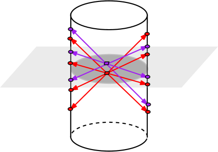
Figure 10. (a) Diffraction by a grain (incoming and diffraction directions are $s$ and $t,$ respectively); (b) the general indexing problem (determining the grains from diffraction spots).

The limited number of data, and the fact that multiple grains are simultaneously imaged, poses major algorithmic challenges at quite different scales, from the atomic to the macroscopic level. The problem, commonly referred to as indexing [48, 160, 165], is to group the tomographic data according to their grain of origin. This allows often the determination of grain parameters like the lattice (including its orientation), or the center of mass; see Fig. 10(b). Based on the tomographic data acquired for each single grain, the macroscopic geometric structure of the full collection of different grains is then to be determined. Of course, such tasks can be highly interrelated, and there are also possible cases where it is favorable to reconstruct several of the grains simultaneously. More details can be found in [153].

7.2. Macroscopic reconstruction

As in Sect. 5, a single grain $g$ can be considered as a binary image $\psi_{g}\in\mathcal{F}^{3}.$ The points of $\textnormal{supp}(\psi_{g})$ correspond to the pixels that belong to $g$. The paper [167] describes one of the first attempts of reconstructing multiple grains, the so-called grain map. In this paper the ART algorithm is used, but it is found that often the reconstructions contain unrealistic void spaces between adjacent grains. To overcome this problem, a Monte-Carlo approach based on Gibbs priors was introduced in [154]. This approach was generalized in [169] (see also [6]) to deal with the task of reconstructing grain maps of moderately deformed grains. More stochastic approaches to grain map reconstruction can be found in [159, 161, 162, 169]. For alternative approaches, see [50, 155, 156, 157, 168, 171, 172].

In the following we describe a linear-programming based method, introduced in [174], which returns approximations of grain maps. It is based on only a few input parameters for each grain: (approximations of) its center-of-mass, its volume and, if available, its second-order moments. The centers-of-mass can be determined by the indexing procedure, the grain volume by integration of the respective X-ray data, and the second-order moments by backprojecting the projections acquired from the same grain.

The aim is to reconstruct what we call generalized balanced power diagrams (GBPDs). These diagrams generalize power diagrams (which are also known as Laguerre or Dirichlet tessellations), which in turn generalize Voronoi diagrams; see also [8] and [9, Sect. 6.2].

Any GBPD is specified by a set of distinct sites $S=\{s_{1},\dots,s_{l}\}\subset\mathbb{R}^{d},$ additive weights $(\sigma_{1},\dots,\sigma_{l})^{T}\in\mathbb{R}^{l},$ and positive definite matrices $A_{1},\dots,A_{l}\in\mathbb{R}^{d\times d}.$ The $j$th generalized balanced power cell $P_{j}$ is then defined by

$$P_{j}=\{x\in\mathbb{R}^{d}\>:\>||x-s_{j}||_{A_{j}}^{2}-\sigma_{j}\leq||x-s_{k}||_{A_{k}}^{2}-\sigma_{k},\>\forall k\neq j\},$$

where $||\cdot||_{A_{j}},$ $j\in[l],$ denotes the ellipsoidal norm

$$||x||_{A_{j}}=\sqrt{x^{T}A_{j}x}.$$

The generalized balanced power diagram $P$ is the $l$-tuple $P=(P_{1},\dots,P_{l})$. The proposed method is able to find optimal $\sigma_{1},\dots,\sigma_{l}$ that guarantee that the volumes of each cell are within prescribed ranges.

The concept of GBPDs can be viewed as structure-driven weight balanced clusterings; see [176, 177]. For $j\in[l]$ let $s_{j}$ denote the center of the $j$th grain, and let $\kappa_{j}^{-},$ $\kappa_{j}^{+}$ be lower and upper bounds for its volume, respectively. Further, let $x_{1},\dots,x_{q}$ be the points of the image that has to be partitioned into the grains, and set $\gamma_{i,j}=||x_{i}-s_{j}||_{A_{i}}^{2}$ for all $i,j$.

Then we can model the assignment problem by the following linear program:

$$\begin{array}[]{lll}\displaystyle\textnormal{(LP)}&\displaystyle\min\sum_{i=1}^{q}\sum_{j=1}^{l}\gamma_{i,j}\xi_{i,j}&\\ \displaystyle\textnormal{subject to}&\displaystyle\sum_{j=1}^{l}\xi_{i,j}=1&\displaystyle(i\in[q]),\\ \displaystyle&\displaystyle\kappa_{j}^{-}\leq\sum_{i=1}^{q}\xi_{i,j}\leq\kappa_{j}^{+}&\displaystyle(j\in[l]),\\[17.22217pt] \displaystyle&\displaystyle\xi_{i,j}\geq 0&\displaystyle(i\in[q];\>j\in[l]).\end{array}$$

In general, the variables $\xi_{i,j}$ specify the fraction of the point $x_{i}$ that is assigned to the center $s_{j}.$ Since, however, the coefficient matrix is totally unimodular all basic feasible solutions are binary, and we obtain an optimal assignment of pixels to grains in polynomial time.

An example for the quality of reconstruction for planar grain maps (which are easier to visualize) is shown in Fig. 11. Reports on the favorable performance of the presented approach on various (real-world) data sets can be found in the recent papers [178, 179, 180, 181, 182].

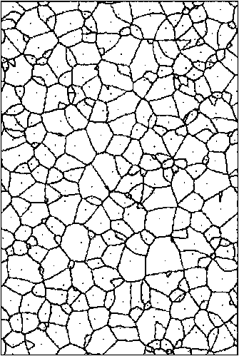
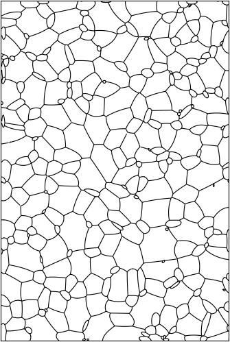
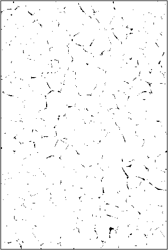
Figure 11. (a) Original image from [17, Fig. 9.7]. (Black dots represent grain centers.) (b) Reconstructed generalized balanced power diagram. (c) Difference map. (Black pixels indicate the pixels that are black in (b) but white in (a)).

We remark that the clustering approach described above was previously applied (in an ‘isotropic’ fashion) in the context of farmland consolidation [12, 175]. For an application in designing electoral districts where municipalities of a state have to be grouped into districts of nearly equal population while obeying certain politically motivated requirements, see [177].

8. Switching components and a problem in number theory

Switching components, i.e., pairs of tomographically equivalent sets as introduced in Sect. 3.1, are strongly related to an old problem in Diophantine number theory, called the Prouhet-Tarry-Escott or PTE-problem, named after Eugène Prouhet [210], Gaston Tarry [213], and Edward B. Escott [195].

Problem 5 (Prouhet, 1851; Tarry, 1912; Escott, 1910).

Given $k,n\in\mathbb{N},$ find two different multisets $X=\{\xi_{1},\dots,\xi_{n}\}\subset\mathbb{Z}$ and $Y=\{\eta_{1},\dots,\eta_{n}\}\subset\mathbb{Z},$ such that

$$\xi_{1}^{j}+\xi_{2}^{j}+\ldots+\xi_{n}^{j}=\eta_{1}^{j}+\eta_{2}^{j}+\ldots+\eta_{n}^{j},\qquad\textnormal{for }j\in[k].$$

Pairs $(X,Y)$ satisfying the above equation are called PTE solutions. More precisely, we speak of $(k,n)$-solutions, and the numbers $k$ and $n,$ respectively, are referred to as the degree and size of the PTE solution. Often the notation $X\stackrel{{\scriptstyle k}}{{=}}Y$ is used to indicate that $(X,Y)$ is a degree $k$ solution. For instance, as an elementary calculation shows,

$$\{0,14,28,56,70,84\}\stackrel{{\scriptstyle 5}}{{=}}\{4,6,40,44,78,80\}.$$

The PTE problem has connections to several other problems in number theory, including the ‘easier’ Waring problem [214, 217], [13, Sect. 12], the Hilbert-Kamke problem [200, 201], and a conjecture due to Erdős and Szekeres [193, 194, 203], [13, Sect. 13]. There are also connections to Ramanujan identities [205, 209], other types of multigrade equations [192, 211], problems in algebra [204, 207], geometry [196], combinatorics [184, 185, 188, 191], graph theory [199], and computer science [189, 190, 197]. For background information see [5, 13, 14, 19, 24].

The PTE problem can be traced back to a correspondence between Goldbach and Euler. In his 1950 letter [198] Goldbach states the identity

$$(\alpha+\beta+\delta)^{2}+(\alpha+\gamma+\delta)^{2}+(\beta+\gamma+\delta)^{2}+\delta^{2}\\ =(\alpha+\delta)^{2}+(\beta+\delta)^{2}+(\gamma+\delta)^{2}+(\alpha+\beta+\gamma+\delta)^{2},$$

where $\alpha,\beta,\gamma,\delta\in\mathbb{Z}.$ In other words,

$$\{\alpha+\beta+\delta,\alpha+\gamma+\delta,\beta+\gamma+\delta,\delta\}\stackrel{{\scriptstyle 2}}{{=}}\{\alpha+\delta,\beta+\delta,\gamma+\delta,\alpha+\beta+\gamma+\delta\}.$$

It was already known to Prouhet, Tarry, and Escott that there exist $(k,2^{k})$-solutions for every $k$ (see [216] and [19, Sect. 24]). Such solutions can be generated as follows. Express each $p\in[2^{k+1}-1]_{0}$ as a binary number. If this binary expression of $p$ contains an even number of $1$’s, then assign $p$ to the set $X,$ otherwise to $Y.$ Then, $(X,Y)$ with $X=\{\xi_{1},\dots,\xi_{2^{k}}\}$ and $Y=\{\eta_{1},\dots,\eta_{2^{k}}\}$ is a $(k,2^{k})$-solution. Proofs of this result can be found in [208, 216]. For generalizations, see [202, 212].

On the other hand, there are no $(k,n)$-solutions whenever $n<k+1.$ This result, commonly attributed to Bastien [187], can be derived from the Newton’s identities [32, Sect. 21.9]. A $(k,n)$-solution is called ideal if $n=k+1.$

The following is a long-standing open question (see [215] and [13, Sect. 11]).

Problem 6.

Do there exist ideal PTE solutions for every $k?$

Presently, ideal solutions are only known for $k\in[11]\setminus\{10\}.$ Concerning upper bounds on $n,$ the currently best bound (of [206]) guarantees that for any $k$ there exists a $(k,n)$-solution with $n\leq\frac{1}{2}(k^{2}-3)$ if $k$ is odd and $n\leq\frac{1}{2}(k^{2}-4)$ if $k$ is even. The proofs are non-constructive. In fact, all currently known constructive proofs yield bounds that are exponential in $k.$

8.1. PTE solutions from switching components

The following explicit connection between the PTE problem and switching components first appeared in [3, Sect. 6]. Following [186], we will focus on the case $d=2$ (for general $d$ see [63]).

For given $M\subset\mathbb{Z}^{d}$ and $c\in\mathbb{Z}^{d},$ let $\Pi_{c}(M)$ denote the multiset

$$\Pi_{c}(M)=\{c^{T}x\>:\>x\in X\}.$$

Clearly, $\Pi_{c}(M)\subset\mathbb{Z}.$ Perhaps more surprisingly, the following result holds if we insert the points of a switching component.

Theorem 24 ([186]).

If $(X,Y)$ is an $(m+1)$-switching component in $\mathbb{Z}^{2}$ and $c\in\mathbb{Z}^{2}$ such that $\Pi_{c}(X)\neq\Pi_{c}(Y),$ then $(\Pi_{c}(X),\Pi_{c}(Y))$ is a degree $m$ solution of the PTE problem.

This construction of PTE-solutions from switching components can be exemplified, say, for the switching components depicted in Fig. 12.

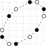
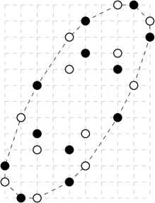
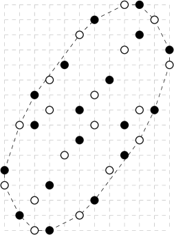
Figure 12. Examples of small switching components for (a) $m=6,$ (b) $m=7,$ (c) $m=8,$ (d) $m=9,$ directions (indicated as polygon edges). The switching components are the sets of $6,$ $10,$ $12,$ and $18$ black and white points, respectively.

For instance, if in Fig. 12(a) the origin is located in the lower left lattice point (which, of course, is an arbitrary choice) the sets $X$ and $Y$ of black and white points are

$$\begin{array}[]{lll}X&=&\left\{\left(\begin{array}[]{c}0\\ 2\end{array}\right),\left(\begin{array}[]{c}1\\ 0\end{array}\right),\left(\begin{array}[]{c}2\\ 5\end{array}\right),\left(\begin{array}[]{c}4\\ 1\end{array}\right),\left(\begin{array}[]{c}5\\ 6\end{array}\right),\left(\begin{array}[]{c}6\\ 4\end{array}\right)\right\},\\[8.61108pt] Y&=&\left\{\left(\begin{array}[]{c}0\\ 1\end{array}\right),\left(\begin{array}[]{c}1\\ 4\end{array}\right),\left(\begin{array}[]{c}2\\ 0\end{array}\right),\left(\begin{array}[]{c}4\\ 6\end{array}\right),\left(\begin{array}[]{c}5\\ 2\end{array}\right),\left(\begin{array}[]{c}6\\ 5\end{array}\right)\right\}.\end{array}$$

For $c^{T}=(1,2)$ we obtain the PTE solution

$$\Pi_{c}(X)=\{1,4,6,12,14,17\}\stackrel{{\scriptstyle 5}}{{=}}\{2,2,9,9,16,16\}=\Pi_{c}(Y)$$

of degree 5. As a basic ingredient the standard proof of Thm. 24 uses the encoding of points by polynomials mentioned in connection with Thm. 7.

Thm. 24 allows to derive explicit constructions of families of PTE solutions; [186]). As an example let us consider the result of Prouhet, Tarry, and Escott that $(k,2^{k})$-solutions exist for every $k.$ The proof given in [215] extends over two half-pages. The geometric shortcut via Thm. 24 just uses the construction of switching components $(X,Y)$ with $|X|=|Y|\leq 2^{k}$ from Fig. 2.

8.2. Generalizations

The geometric point of view also helps in studying other variants of the PTE problem. Naturally, PTE can be considered over arbitrary rings $R$. For $R=\mathbb{Z}^{d}$ we obtain PTE_d which can be viewed as a $d$-dimensional or multinomial version of the original PTE problem.

Problem 7 (PTE_d).

Given $d,k,n\in\mathbb{N},$ find two different multisets $X=\{\xi_{1},\dots,\xi_{n}\},$ $Y=\{\eta_{1},\dots,\eta_{n}\}\subset\mathbb{Z}^{d}$ with $\xi_{l}=(\xi_{l1},\dots,\xi_{ld})^{T},$ $\eta_{l}=(\eta_{l1},\dots,\eta_{ld})^{T}$ for $l\in[n]$ such that

$$\sum_{l=1}^{n}\xi_{l1}^{j_{1}}\xi_{l2}^{j_{2}}\cdot\ldots\cdot\xi_{ld}^{j_{d}}=\sum_{l=1}^{n}\eta_{l1}^{j_{1}}\eta_{l2}^{j_{2}}\cdot\ldots\cdot\eta_{ld}^{j_{d}}$$

for all non-negative integers $j_{1},\dots,j_{d}$ with $j_{1}+j_{2}+\ldots+j_{d}\leq k.$

There are trivial ways of generating PTE_d-solution from PTE₁-solutions. For instance, if $\{\alpha_{1},\dots,\alpha_{n}\}\stackrel{{\scriptstyle k}}{{=}}\{\beta_{1},\dots,\beta_{n}\}$ is a PTE₁-solution, then

$$\{(\alpha_{1},\dots,\alpha_{1})^{T},\dots,(\alpha_{n},\dots,\alpha_{n})^{T}\}\stackrel{{\scriptstyle k}}{{=}}\{(\beta_{1},\dots,\beta_{1})^{T},\dots,(\beta_{n},\dots,\beta_{n})^{T}\}$$

is a solution to PTE${}_{d}.$ A general method of generating non-trivial solutions for PTE₂ is provided by [186].

Theorem 25 ([186]).

Every $(m+1)$-switching component $(X,Y)$ in $\mathbb{Z}^{2},$ is a degree $m$ solution of the PTE₂ problem.

For instance, for the sets $X$ and $Y$ corresponding to Fig. 12(a) it is elementary to verify that

$$0^{i}2^{j}+1^{i}0^{j}+2^{i}5^{j}+ 4^{i}1^{j}+5^{i}6^{j}+6^{i}4^{j}$$

$$=0^{i}1^{j}+1^{i}4^{j}+2^{i}0^{j}+4^{i}6^{j}+5^{i}2^{j}+6^{i}5^{j}$$

for all non-negative $i,j$ with $i+j\leq 5.$

Applying Thm. 25 to the known smallest size switching components (an example for $k+1=6$ is depicted in Fig. 12(a)), one sees that for every degree $k\in\{1,2,3,5\}$ there exist ideal PTE₂ solutions; [186].

The following problem is, however, open already for $k=4.$

Problem 8.

Do there exist ideal PTE₂ for every degree $k$?

9. Concluding remarks

The present paper tried to support the following conviction of the authors: Discrete tomography is a broad and interesting field, both, in terms of its methods and its applications. Discrete tomography has strong links to various areas within mathematics which have the potential to provide new insight in older problems. Discrete tomography has a variety of applications to various other scientific fields and to relevant real-world problems. And, finally, discrete tomography is a rich source of scientific challenges.

References

- [1] []General reading: Introductions, surveys, books:
- [2] R. J. Adrian and J. Westerweel. Particle Image Velocimetry. Cambridge University Press, New York, NY, 2010.
- [3] A. Alpers. Instability and Stability in Discrete Tomography. PhD thesis, Technische Universität München, Zentrum Mathematik, 2003. (published by Shaker Verlag, ISBN 3-8322-2355-X).
- [4] A. Alpers. A short introduction to tomographic grain map reconstruction. PU.M.A., 20(1-2):157–163, 2009. URL: http://puma.dimai.unifi.it/20_1_2/10_Alpers_7.pdf.
- [5] A. Alpers. On the Tomography of Discrete Structures: Mathematics, Complexity, Algorithms, and its Applications in Materials Science and Plasma Physics. Habilitation thesis, Technische Universität München, Zentrum Mathematik, 2018. URL: http://mediatum.ub.tum.de/1441933.
- [6] A. Alpers, L. Rodek, H. F. Poulsen, E. Knudsen, and G. T. Herman. Discrete tomography for generating grain maps of polycrystals. In G. T. Herman and A. Kuba, editors, Advances in Discrete Tomography and its Applications, pages 271–301. Birkhäuser, Boston, 2007. doi:10.1007/978-0-8176-4543-4_13.
- [7] R. C. Aster, B. Borchers, and C. H. Thurber. Parameter Estimation and Inverse Problems. Academic Press, Boston, MA, 2nd edition edition, 2013. doi:10.1016/B978-0-12-385048-5.00030-6.
- [8] F. Aurenhammer. Power diagrams: Properties, algorithms and applications. SIAM J. Comput., 16(1):78–96, 1987. doi:10.1137/0216006.
- [9] F. Aurenhammer, R. Klein, and D.-T. Lee. Voronoi Diagrams and Delaunay Triangulations. World Scientific, Singapore, 2013.
- [10] S. Bals, B. Goris, A. De Backer, S. Van Aert, and G. Van Tendeloo. Atomic resolution electron tomography. MRS Bulletin, 41(7):525–530, 2016. doi:10.1557/mrs.2016.138.
- [11] J. Banhart, editor. Advanced Tomographic Methods in Materials Research and Engineering. Oxford University Press, Oxford, 2008.
- [12] S. Borgwardt, A. Brieden, and P. Gritzmann. Geometric clustering for the consolidation of farmland and woodland. Math. Intell., 36(2):37–44, 2014. doi:10.1007/s00283-014-9448-2.
- [13] P. Borwein. Computational Excursions in Analysis and Number Theory. Springer, New York, NY, 2002. doi:10.1007/978-0-387-21652-2.
- [14] P. Borwein and C. Ingalls. The Prouhet-Tarry-Escott problem revisited. Enseign. Math., 40(1-2):3–27, 1994. doi:10.5169/seals-61102.
- [15] R. A. Brualdi. Combinatorial Matrix Classes. Cambridge University Press, Cambridge, 2006.
- [16] R. Burkard, M. Dell’Amico, and S. Martello. Assignment Problems. SIAM, Philadelphia, PA, 2009. doi:10.1137/1.9781611972238.
- [17] S. N. Chiu, D. Stoyan, W. S. Kendall, and J. Mecke. Stochastic Geometry and its Applications. Wiley, Chichester, 3rd edition edition, 2013.
- [18] A. Del Lungo and M. Nivat. Reconstruction of connected sets from two projections. In G. T. Herman and A. Kuba, editors, Discrete Tomography, pages 163–188. Birkhäuser, Boston, 1999. doi:10.1007/978-1-4612-1568-4_7.
- [19] L. E. Dickson. History of the Theory of Numbers, volume 2. Dover Publications, Mineola, NY, 1920.
- [20] L. Gan and G. J. Jensen. Electron tomography of cells. Q. Rev. Biophys., 45(1):27–56, 2012. doi:10.1017/S0033583511000102.
- [21] R. J. Gardner. Geometric Tomography. Cambridge University Press, New York, NY, 2nd edition edition, 2006. doi:10.1017/CBO9781107341029.
- [22] R. J. Gardner and P. Gritzmann. Uniqueness and complexity in discrete tomography. In G. T. Herman and A. Kuba, editors, Discrete Tomography, pages 85–113. Birkhäuser, Boston, 1999. doi:10.1007/978-1-4612-1568-4_4.
- [23] M. R. Garey and D. S. Johnson. Computers and Intractability. W. H. Freeman and Co., San Francisco, CA, 1979.
- [24] A. Gloden. Mehrgradige Gleichungen. P. Noordhoff, Groningen, 2nd edition edition, 1943.
- [25] U. Grimm, P. Gritzmann, and C. Huck. Discrete tomography of model sets: Reconstruction and uniqueness. In M. Baake and U. Grimm, editors, Aperiodic Order, volume 2, pages 39–72. Cambridge University Press, Cambridge, 2017. doi:10.1017/9781139033862.004.
- [26] P. Gritzmann. On the reconstruction of finite lattice sets from their X-rays. In E. Ahronovitz and C. Fiorio, editors, Discrete Geometry for Computer Imagery, pages 19–32. Springer, Berlin, 1997. doi:10.1007/BFb0024827.
- [27] P. Gritzmann. Discrete tomography: From battleship to nanotechnology. In Aignern M. and E. Behrends, editors, Mathematics Everywhere, pages 81–98. American Mathematical Society, 2010. doi:10.1136/bmj.c3793.
- [28] P. Gritzmann and S. de Vries. Reconstructing crystalline structures from few images under high resolution transmission electron microscopy. In W. Jäger and H. J. Krebs, editors, Mathematics: Key Technology for the Future, pages 441–459. Springer, Berlin, 2003. doi:10.1007/978-3-642-55753-8_36.
- [29] J. Hadamard. Lectures on the Cauchy Problem in Linear Partial Differential Equations. Dover Publications Inc., Mineola, NY, 1952. Reprint of the 1923 original.
- [30] L. Hajdu and R. Tijdeman. Algebraic discrete tomography. In G. T. Herman and A. Kuba, editors, Advances in Discrete Tomography and its Applications, pages 55–81. Birkhäuser, Boston, 2007. doi:10.1007/978-0-8176-4543-4_4.
- [31] P. C. Hansen. Discrete Inverse Problems: Insight and Algorithms. SIAM, Philadelphia, PA, 2010. doi:10.1137/1.9780898718836.
- [32] G. H. Hardy and E. M. Wright. An Introduction to the Theory of Numbers. Oxford University Press, Oxford, 6th edition edition, 2008.
- [33] G. T. Herman. Fundamentals of Computerized Tomography: Image Reconstruction from Projections. Springer, London, 2nd edition edition, 2009. doi:10.1007/978-1-84628-723-7.
- [34] G. T. Herman. Iterative reconstruction techniques and their superiorization for the inversion of the Radon transform. In O. Scherzer and R. Ramlau, editors, The Radon Transform: The First 100 Years and Beyond, pages ??–?? De Gruyter, Berlin, 2019.
- [35] G. T. Herman and J. Frank, editors. Computational Methods for Three-Dimensional Microscopy Reconstruction. Springer, New York, NY, 2014. doi:10.1007/978-1-4614-9521-5.
- [36] G. T. Herman and A. Kuba, editors. Discrete Tomography: Foundations, Algorithms, and Applications. Birkhäuser, Boston, MA, 1999. doi:10.1007/978-1-4612-1568-4.
- [37] G. T. Herman and A. Kuba, editors. Advances in Discrete Tomography and its Applications. Birkhäuser, Boston, MA, 2007. doi:10.1007/978-0-8176-4543-4.
- [38] M. B. Katz. Questions of Uniqueness and Resolution in Reconstruction from Projections. Springer, Berlin, 1978. doi:10.1007/978-3-642-45507-0.
- [39] A. Kirsch. An Introduction to the Mathematical Theory of Inverse Problems. Springer, New York, NY, 2011. doi:10.1007/978-1-4419-8474-6.
- [40] U. F. Kocks, C. N. Tomé, and H.-R. Wenk. Texture and Anisotropy: Preferred Orientations in Polycrystals and their Effect on Materials Properties. Cambridge University Press, Cambridge, 2000.
- [41] A. K. Louis. Uncertainty, ghosts and resolution in Radon problems. In O. Scherzer and R. Ramlau, editors, The Radon Transform: The First 100 Years and Beyond, pages ??–?? De Gruyter, Berlin, 2019.
- [42] A. Markoe. Analytic Tomography. Cambridge University Press, New York, NY, 2014. doi:10.1017/CBO9780511530012.
- [43] J. L. Mueller and S. Siltanen. Linear and Nonlinear Inverse Problems with Practical Applications. SIAM, Philadelphia, PA, 2012. doi:10.1137/1.9781611972344.
- [44] F. Natterer. The Mathematics of Computerized Tomography. SIAM, Philadelphia, PA, 2001. doi:10.1137/1.9780898719284.
- [45] F. Natterer and F. Wübbeling. Mathematical Methods in Image Reconstruction. SIAM, Philadelphia, PA, 2001. doi:10.1137/1.9780898718324.
- [46] O. Öktem. Mathematics of electron tomography. In O. Scherzer, editor, Handbook of Mathematical Methods in Imaging, pages 937–1031. Springer, New York, NY, 2nd edition edition, 2015. doi:10.1007/978-3-642-27795-5_43-2.
- [47] C. H. Papadimitriou. Computational Complexity. Addison-Wesley, Reading, MA, 1995.
- [48] H. F. Poulsen. Three-Dimensional X-ray Diffraction Microscopy. Springer, Berlin, 2004.
- [49] H. F. Poulsen. An introduction to three-dimensional X-ray diffraction microscopy. J. Appl. Cryst., 45(6):1084–1097, 2012. doi:10.1107/S0021889812039143.
- [50] H. F. Poulsen, S. Schmidt, D. Juul Jensen, H. O. Sørensen, E. M. Lauridsen, U. L. Olsen, W. Ludwig, A. King, J. P. Wright, and G. B. M. Vaughan. 3D X-ray diffraction microscopy. In R. Barabash and G. Ice, editors, Strain and Dislocation Gradients from Diffraction: Spatially-Resolved Local Structure and Defects, pages 205–253. World Scientific, Singapore, 2014.
- [51] L. Priester. Grain Boundaries: From Theory to Engineering. Springer, Dordrecht, 2013. doi:10.1007/978-94-007-4969-6.
- [52] H. J. Ryser. Combinatorial properties of matrices of zeros and ones. Canad. J. Math., 9(1):371–377, 1957. doi:10.1007/978-0-8176-4842-8_18.
- [53] H. J. Ryser. Combinatorial Mathematics. MAA, Washington, DC, 1963.
- [54] A. Schrijver. Theory of Linear and Integer Programming. Wiley, Chichester, 1986.
- [55] A. Schröder and C. E. Willert, editors. Particle Image Velocimetry. Springer, Berlin, 2008. doi:10.1007/978-3-540-73528-1.
- [56] D. J. Smith. Progress and perspectives for atomic-resolution electron microscopy. Ultramicroscopy, 108(3):159–166, 2018. doi:10.1016/j.ultramic.2007.08.015.
- [57] J. C. H. Spence. High-Resolution Electron Microscopy, volume 4. Oxford Univ. Press, Oxford, 2013. doi:10.1093/acprof:oso/9780199668632.001.0001.
- [58] A. Tarantola. Inverse Problem Theory and Methods for Model Parameter Estimation. SIAM, Philadelphia, PA, 2005.
- [59] []Citations in tomography:
- [60] R. Aharoni, G. T. Herman, and A. Kuba. Binary vectors partially determined by linear equation systems. Discrete Math., 171(1-3):1–16, 1997. doi:10.1016/S0012-365X(96)00068-4.
- [61] A. Alpers and S. Brunetti. On the stability of reconstructing lattice sets from X-rays along two directions. In Discrete Geometry for Computer Imagery, LNCS 3429, pages 92–103. Springer, Berlin, 2005. doi:10.1007/978-3-540-31965-8_9.
- [62] A. Alpers, R. J. Gardner, S. König, R. S. Pennington, C. B. Boothroyd, L. Houben, R. E. Dunin-Borkowski, and K. J. Batenburg. Geometric reconstruction methods for electron tomography. Ultramicroscopy, 128(C):42–54, 2013. doi:10.1016/j.ultramic.2013.01.002.
- [63] A. Alpers, V. Ghiglione, and P. Gritzmann. On the geometry of switching components. in preparation, 2018.
- [64] A. Alpers and P. Gritzmann. On stability, error correction, and noise compensation in discrete tomography. SIAM J. Discrete Math., 20(1):227–239, 2006. doi:10.1137/040617443.
- [65] A. Alpers and P. Gritzmann. Reconstructing binary matrices under window constraints from their row and column sums. Fund. Inf., 155(4):321–340, 2017. doi:10.3233/FI-2017-1588.
- [66] A. Alpers and P. Gritzmann. Dynamic discrete tomography. Inverse Probl., 34(3):034003 (26pp), 2018. doi:10.1088/1361-6420/aaa202.
- [67] A. Alpers and P. Gritzmann. On double-resolution imaging and discrete tomography. SIAM J. Discrete Math., 32(2):1369–1399, 2018. doi:10.1137/17M1115629.
- [68] A. Alpers, P. Gritzmann, and L. Thorens. Stability and instability in discrete tomography. In Digital and Image Geometry, volume 2243 of LNCS 2243, pages 175–186. Springer, Berlin, 2001. doi:10.1007/3-540-45576-0_11.
- [69] A. Alpers and D. G. Larman. The smallest sets of points not determined by their X-rays. Bull. London Math. Soc., 47(1):171–176, 2015. doi:10.1112/blms/bdu111.
- [70] A. Bains and T. Biedl. Reconstructing -convex multi-coloured polyominoes. Theor. Comput. Sci., 411(34-36):3123–3128, 2010. doi:10.1016/j.tcs.2010.04.041.
- [71] S. Bals, K. J. Batenburg, J. Verbeeck, J. Sijbers, and G. Van Tendeloo. Quantitative three-dimensional reconstruction of catalyst particles for bamboo-like carbon-nanotubes. Nano Lett., 7(12):3669–3674, 2007. doi:10.1021/nl071899m.
- [72] E. Barcucci, A. Del Lungo, M. Nivat, and R. Pinzani. X-rays characterizing some classes of discrete sets. Linear Algebra Appl., 339(1-3):3–21, 2001. doi:10.1016/S0024-3795(01)00431-1.
- [73] E. Barcucci, P. Dulio, A. Frosini, and S. Rinaldi. Ambiguity results in the characterization of -convex polyominoes from projections. In Discrete Geometry for Computer Imagery, LNCS 10502, pages 147–158. Springer, Berlin, 2017. doi:10.1007/978-3-319-66272-5_13.
- [74] K. J. Batenburg, S. Bals, S. Sijbers, C. Kuebel, P. A. Midgley, J. C. Hernandez, U. Kaiser, E. R. Encina, E. A. Coronado, and G. Van Tendeloo. 3D imaging of nanomaterials by discrete tomography. Ultramicroscopy, 109(6):730–740, 2009. doi:10.1016/j.ultramic.2009.01.009.
- [75] K. J. Batenburg and W. A. Kosters. A discrete tomography approach to Japanese puzzles. In Proceedings of the 16th Belgium-Netherlands Conference on Artificial Intelligence (BNAIC), pages 243–250, 2004.
- [76] K. J. Batenburg and J. Sijbers. DART: A practical reconstruction algorithm for discrete tomography. IEEE Trans. Image Process., 20(9):2542–2553, 2011. doi:10.1109/TIP.2011.2131661.
- [77] G. Bianchi and M. Longinetti. Reconstructing plane sets from projections. Discrete Comput. Geom., 5(3):223–242, 1990. doi:10.1007/BF02187787.
- [78] J. Bosboom, E. D. Demaine, M. L. Demaine, A. Hesterberg, R. Kimball, and J. Kopinsky. Path puzzles: Discrete tomography with a path constraint is hard. 2018. URL: http://arxiv.org/abs/1803.01176.
- [79] S. Brunetti and A. Daurat. An algorithm reconstructing convex lattice sets. Theor. Comput. Sci., 304(1-3):35–57, 2003. doi:10.1016/S0304-3975(03)00050-1.
- [80] S. Brunetti and A. Daurat. Reconstruction of convex lattice sets from tomographic projections in quartic time. Theor. Comput. Sci., 406(1-2):55–62, 2008. doi:10.1016/j.tcs.2008.06.003.
- [81] S. Brunetti, A. Del Lungo, P. Gritzmann, and S. de Vries. On the reconstruction of binary and permutation matrices under (binary) tomographic constraints. Theor. Comput. Sci., 406(1-2):63–71, 2008. doi:10.1016/j.tcs.2008.06.014.
- [82] S. Brunetti, P. Dulio, L. Hajdu, and C. Peri. Ghosts in discrete tomography. J. Math. Imaging Vision, 53(2):210–224, 2015. doi:10.1007/s10851-015-0571-2.
- [83] S. Brunetti, P. Dulio, and C. Peri. Discrete tomography determination of bounded sets in . Discrete Appl. Math., 183:20–30, 2015. doi:10.1016/j.dam.2014.01.016.
- [84] M. Burger, H. Dirks, L. Frerking, T. Hauptmann, A. Helin, and S. Siltanen. A variational reconstruction method for undersampled dynamic X-ray tomography based on physical motion models. Inverse Probl., 33(12):124008, 2017. doi:10.1088/1361-6420/aa99cf.
- [85] A. Chambolle. An algorithm for total variation minimization and applications. J. Math. Imaging Vision, 20(1):89–97, 2004. doi:10.1023/B:JMIV.0000011325.36760.1e.
- [86] S-K. Chang. The reconstruction of binary patterns from their projections. Comm. ACM, 14(1):21–25, 1971. doi:10.1145/362452.362471.
- [87] M. J. Chlond. Classroom exercises in IP modeling: Su Doku and the Log Pile. INFORMS Trans. Ed., 5(2):77–79, 2005. doi:10.1287/ited.5.2.77.
- [88] A. Daurat. Determination of Q-convex sets by X-rays. Theor. Comput. Sci., 332(1-3):19–45, 2005. doi:10.1016/j.tcs.2004.10.001.
- [89] D. de Werra, M. C. Costa, C. Picouleau, and B. Ries. On the use of graphs in discrete tomography. 4OR, 6(2):101–123, 2008. doi:10.1007/s10288-008-0077-5.
- [90] J. Diemunsch, M. Ferrara, S. Jahanbekam, and J. M. Shook. Extremal theorems for degree sequence packing and the two-color discrete tomography problem. SIAM J. Discrete Math., 29(4):2088–2099, 2015. doi:10.1137/140987912.
- [91] P. Dulio, R. J. Gardner, and C. Peri. Discrete point X-rays. SIAM J. Discrete Math., 20(1):171–188, 2006. doi:10.1137/040621375.
- [92] P. Dulio and C. Peri. Discrete tomography and plane partitions. Adv. Appl. Math., 50(3):390–408, 2013. doi:10.1016/j.aam.2012.10.005.
- [93] C. Dürr. Discrete tomography applets. Accessed: 2018-09. URL: http://www-desir.lip6.fr/~durrc/Xray/Complexity/#DGM.
- [94] C. Dürr, F. Guiñez, and M. Matamala. Reconstructing 3-colored grids from horizontal and vertical projections is NP-hard: A solution to the 2-atom problem in discrete tomography. SIAM J. Discrete Math., 26(1):330–352, 2012. doi:10.1137/100799733.
- [95] P. C Fishburn, J. C Lagarias, J. A. Reeds, and L. A. Shepp. Sets uniquely determined by projections on axes II: Discrete case. Discrete Math., 91(2):149–159, 1991. doi:10.1016/0012-365X(91)90106-C.
- [96] D. Gale. A theorem on flows in networks. Pacific J. Math., 7(2):1073–1082, 1957.
- [97] R. J. Gardner. Geometric tomography website. Accessed: 2018-09. URL: http://www.geometrictomography.com/.
- [98] R. J. Gardner and P. Gritzmann. Discrete tomography: Determination of finite sets by -rays. Trans. Amer. Math. Soc., 349(6):2271–2295, 1997. doi:10.1090/S0002-9947-97-01741-8.
- [99] R. J. Gardner, P. Gritzmann, and D. Prangenberg. On the reconstruction of binary images from their discrete Radon transform. In R. A. Melter, A. Y. Wu, and L. Latecki, editors, Vision Geometry V, SPIE Proc. 2826, pages 121–132. Society of Photo-Optical Instrumentation Engineers, Denver, CO, 1996. doi:10.1117/12.251785.
- [100] R. J. Gardner, P. Gritzmann, and D. Prangenberg. On the computational complexity of reconstructing lattice sets from their X-rays. Discrete Math., 202(1-3):45–71, 1999. doi:10.1016/S0012-365X(98)00347-1.
- [101] R. J. Gardner, P. Gritzmann, and D. Prangenberg. On the computational complexity of determining polyatomic structures by X-rays. Theoret. Comput. Sci., 233(1-2):91–106, 2000. doi:10.1016/S0304-3975(97)00298-3.
- [102] R. J. Gardner and P. McMullen. On Hammer’s X-ray problem. J. London Math. Soc. (2), 21(1):171–175, 1980. doi:10.1112/jlms/s2-21.1.171.
- [103] P. Gritzmann and S. de Vries. On the algorithmic inversion of the discrete Radon transform. Theor. Comput. Sci., 281(1-2):455–469, 2002. doi:10.1016/S0304-3975(02)00023-3.
- [104] P. Gritzmann, B. Langfeld, and M. Wiegelmann. Uniqueness in discrete tomography: Three remarks and a corollary. SIAM J. Discrete Math., 25(4):1589–1599, 2011. doi:10.1137/100803262.
- [105] P. Gritzmann, D. Prangenberg, S. de Vries, and M. Wiegelmann. Success and failure of certain reconstruction and uniqueness algorithms in discrete tomography. Int. J. Imaging Syst. Technol., 9(2-3):101–109, 1998. doi:10.1002/(SICI)1098-1098(1998)9:2/3<101::AID-IMA6>3.0.CO;2-F.
- [106] B. Hahn. Reconstruction of dynamic objects with affine deformations in computerized tomography. J. Inverse Ill-Posed Probl., 22(3):323–339, 2014. doi:10.1515/jip-2012-0094.
- [107] L. Hajdu and R. Tijdeman. Algebraic aspects of discrete tomography. J. Reine Angew. Math., 534:119–128, 2001. doi:10.1515/crll.2001.037.
- [108] A. Heppes. On the determination of probability distributions of more dimensions by their projections. Acta Math. Acad. Sci. Hung., 7(3-4):403–410, 1956. doi:10.1007/BF02020535.
- [109] G. T. Herman. Reconstruction of binary patterns from a few projections. In A. Günther, B. Levrat, and H. Lipps, editors, International Computing Symposium 1973, pages 371–378. North-Holland, Amsterdam, 1974.
- [110] L. Houben and M. Bar Sadan. Refinement procedure for the image alignment in high-resolution electron tomography. Ultramicroscopy, 111(9-10):1512–1520, 2011. doi:10.1016/j.ultramic.2011.06.001.
- [111] C. Huck. Solution of a uniqueness problem in the discrete tomography of algebraic Delone sets. J. Reine Angew. Math., 677:199–224, 2013. doi:10.1515/crelle.2012.026.
- [112] R. W. Irving and M. R. Jerrum. Three-dimensional statistical data security problems. SIAM J. Comput., 23(1):170–184, 1994. doi:10.1137/S0097539790191010.
- [113] C. L. Jia, S. B. Mi, J. Barthel, D. W. Wang, R. E. Dunin-Borkowski, K. W. Urban, and A. Thust. Determination of the 3D shape of a nanoscale crystal with atomic resolution from a single image. Nat. Mater., 13:1044–1049, 2014. doi:10.1038/nmat4087.
- [114] J. R. Jinschek, K. J. Batenburg, H. A. Calderon, R. Kilaas, V. Radmilovic, and C. Kisielowski. 3-D reconstruction of the atomic positions in a simulated gold nanocrystal based on discrete tomography: Prospects of atomic resolution electron tomography. Ultramicroscopy, 108(6):589–604, 2008. doi:10.1016/j.ultramic.2007.10.002.
- [115] C. Kisielowski, P. Schwander, F. H. Baumann, M. Seibt, Y. Kim, and A. Ourmazd. An approach to quantitative high-resolution transmission electron microscopy of crystalline materials. Ultramicroscopy, 58(2):131–155, 1995. doi:10.1016/0304-3991(94)00202-X.
- [116] J. Klukowska, R. Davidi, and G. T. Herman. SNARK09 - A software package for reconstruction of 2D images from 1D projections. Comput. Meth. Prog. Bio., 110(3):424–440, 2013. doi:10.1016/j.cmpb.2013.01.003.
- [117] T. Y. Kong and G. T. Herman. On which grids can tomographic equivalence of binary pictures be characterized in terms of elementary switching operations? Int. J. Imaging Syst. Technol., 9(2-3):118–125, 1998. doi:10.1002/(SICI)1098-1098(1998)9:2/3<118::AID-IMA8>3.0.CO;2-E.
- [118] A. Kuba and A. Volčič. Characterisation of measurable plane sets which are reconstructable from their two projections. Inverse Probl., 4(2):513–527, 1988. doi:10.1088/0266-5611/4/2/014.
- [119] M. Longinetti. Some questions of stability in the reconstruction of plane convex bodies from projections. Inverse Probl., 1(1):87–97, 1985. doi:10.1088/0266-5611/1/1/008.
- [120] G. G. Lorentz. A problem of plane measure. Amer. J. Math., 71(2):417–426, 1949. doi:10.2307/2372255.
- [121] P. Maass. The X-ray transform: Singular value decomposition and resolution. Inverse Probl., 3(4):729–741, 1987. doi:10.1088/0266-5611/3/4/016.
- [122] J. Matoušek, A. Přívětivý, and P. Škovroň. How many points can be reconstructed from k projections? SIAM J. Discrete Math., 22(4):1605–1623, 2008. doi:10.1016/j.endm.2007.07.069.
- [123] A. Rényi. On projections of probability distributions. Acta Math. Acad. Sci. Hungar., 3(3):131–142, 1952. doi:10.1007/BF02022515.
- [124] P. Schwander, C. Kisielowski, F. H. Baumann, Y. Kim, and A. Ourmazd. Mapping projected potential, interfacial roughness, and composition in general crystalline solids by quantitative transmission electron microscopy. Phys. Rev. Lett., 71(25):4150–4153, 1993. doi:10.1103/PhysRevLett.71.4150.
- [125] A. Shliferstein and Y. T. Chien. Switching components and the ambiguity problem in the reconstruction of pictures from their projections. Pattern Recogn., 10(5-6):327–340, 1978. doi:10.1016/0031-3203(78)90004-3.
- [126] A. R. Shliferstein and Y. T. Chien. Some properties of image-processing operations on projection sets obtained from digital pictures. IEEE Trans. Comput., C-26(10):958–970, 1977. doi:10.1109/TC.1977.1674731.
- [127] C. H. Slump and J. J. Gerbrands. A network flow approach to reconstruction of the left ventricle from two projections. Comput. Vision. Graph., 18(1):18–36, 1982. doi:0.1016/0146-664X(82)90097-1.
- [128] K. T. Smith, D. C. Solmon, and S. L. Wagner. Practical and mathematical aspects of the problem of reconstructing objects from radiographs. Bull. Amer. Math. Soc., 83(6):1227–1270, 1977. URL: http://projecteuclid.org/euclid.bams/1183539851.
- [129] I. Svalbe and M. Ceko. Maximal -ghosts and minimal information recovery from projected views of an array. In Discrete Geometry for Computer Imagery, LNCS 10502, pages 135–146. Springer, Cham, 2017. doi:10.1007/978-3-319-66272-5_12.
- [130] I. Svalbe and S. Chandra. Growth of discrete projection ghosts created by iteration. In Discrete Geometry for Computer Imagery, LNCS 6607, pages 406–416. Springer, Heidelberg, 2011. doi:10.1007/978-3-642-19867-0_34.
- [131] I. Svalbe, N. Nazareth, N. Normand, and S. Chandra. On constructing minimal ghosts. In 2010 International Conference on Digital Image Computing: Techniques and Applications, pages 276–281. IEEE, Los Alamitos, 2010. doi:10.1109/DICTA.2010.56.
- [132] I. Svalbe and N. Normand. Properties of minimal ghosts. In Discrete Geometry for Computer Imagery, LNCS 6607, pages 417–428. Springer, Heidelberg, 2011. doi:10.1007/978-3-642-19867-0_35.
- [133] W. Van Aarle, W. J. Palenstijn, J. De Beenhouwer, T. Altantzis, S. Bals, K. J. Batenburg, and J. Sijbers. The ASTRA toolbox: A platform for advanced algorithm development in electron tomography. Ultramicroscopy, 157:35–47, 2015. URL: www.astra-toolbox.com, doi:10.1016/j.ultramic.2015.05.002.
- [134] S. Van Aert, K. J. Batenburg, M. D. Rossell, R. Erni, and G. Van Tendeloo. Three-dimensional atomic imaging of crystalline nanoparticles. Nature, 470(7334):374–376, 2011. doi:10.1038/nature09741.
- [135] B. Van Dalen. Stability results for uniquely determined sets from two directions in discrete tomography. Discrete Math., 309(12):3905–3916, 2009. doi:10.1016/j.disc.2008.11.018.
- [136] A. Volčič. Well-posedness of the Gardner-McMullen reconstruction problem. In Proceedings of Conference on Measure Theory, Oberwolfach, 1983, LNM 1089, pages 199–210, 1984. doi:10.1007/BFb0072615.
- [137] X. Zhuge, W. J. Palenstijn, and K. J. Batenburg. A more robust algorithm for discrete tomography from limited projection data with automated gray value estimation. IEEE Trans. Image Process., 25(1):455–468, 2016. doi:10.1109/TIP.2015.2504869.
- [138] S. Zopf. Construction of switching components. In Discrete Geometry for Computer Imagery, LNCS 4245, pages 157–168. Springer, Berlin, 2006. doi:10.1007/11907350_14.
- [139] []Further reading: Particle tracking:
- [140] R. J. Adrian. Particle-imaging techniques for experimental fluid mechanics. Annu. Rev. Fluid Mech., 23:261–304, 1991. doi:10.1146/annurev.fl.23.010191.001401.
- [141] A. Alpers, P. Gritzmann, D. Moseev, and M. Salewski. 3D particle tracking velocimetry using dynamic discrete tomography. Comput. Phys. Commun., 187(1):130–136, 2015. doi:10.1016/j.cpc.2014.10.022.
- [142] R. Dalitz, S. Petra, and C. Schnörr. Compressed Motion Sensing. In Proc. SSVM, volume 10302 of LNCS, pages 602–613. Springer, 2017. doi:10.1007/978-3-319-58771-4_48.
- [143] G. E. Elsinga, F. Scarano, B. Wieneke, and B. W. Oudheusden. Tomographic particle image velocimetry. Exp. Fluids, 41(6):933–947, 2006. doi:10.1007/s00348-006-0212-z.
- [144] R. A. Jamison, A. Fouras, and R. J. Bryson-Richardson. Cardiac-phase filtering in intracardiac particle image velocimetry. J. Biomed. Opt., 17(3):036007, 2012. doi:10.1117/1.JBO.17.3.036007.
- [145] M. Novara, K. J. Batenburg, and F. Scarano. Motion tracking-enhanced MART for tomographic PIV. Meas. Sci. Technol., 21(3):035401, 2010. doi:10.1088/0957-0233/21/3/035401.
- [146] J. F. Pusztaszeri, P. E. Rensing, and T. M. Liebling. Tracking elementary particles near their primary vertex: A combinatorial approach. J. Global Optim., 9(1):41–64, 1996. doi:10.1007/BF00121750.
- [147] D. Reuss, R. Adrian, and C. Landreth. Two-dimensional velocity measurements in a laminar flame using particle image velocimetry. Combust. Sci. Technol., 67(4-6):73–83, 1986. doi:10.1080/00102208908924062.
- [148] F. C. R. Spieksma and G. J. Woeginger. Geometric three-dimensional assignment problems. European J. Oper. Res., 91(3):611–618, 1996. doi:10.1016/0377-2217(95)00003-8.
- [149] M. Umeyama and S. Matsuki. Measurements of velocity and trajectory of water particle for internal waves in two density layers. Geophys. Res. Lett., 38(3):L03612, 2011. doi:10.1029/2010GL046419.
- [150] J. Williams. Application of tomographic particle image velocimetry to studies of transport in complex (dusty) plasma. Phys. Plasmas, 18(5):050702, 2011. doi:10.1063/1.3587090.
- [151] J. Zhu, J. Gao, A. Ehn, M. Aldén, Z. Li, D. Moseev, Y. Kusano, M. Salewski, A. Alpers, P. Gritzmann, and M. Schwenk. Measurements of 3D slip velocities and plasma column lengths of a gliding arc discharge. Appl. Phys. Lett., 106(4):044101, 2015. doi:10.1063/1.4906928.
- [152] []Further reading: Tomographic grain mapping:
- [153] A. Alpers, P. Gritzmann, C. G. Heise, and A. Taraz. On the mathematics of grain reconstruction I: Modeling and computational complexity. in preparation, 2018.
- [154] A. Alpers, H. F. Poulsen, E. Knudsen, and G. T. Herman. A discrete tomography algorithm for improving the quality of 3DXRD grain maps. J. Appl. Crystallogr., 39(4):582–588, 2006. doi:10.1107/S002188980601939X.
- [155] N. R. Barton and J. V. Bernier. A method for intragranular orientation and lattice strain distribution determination. J. Appl. Crystallogr., 45(6):1145–1155, 2012. doi:10.1107/S0021889812040782.
- [156] K. J. Batenburg, J. Sijbers, H. F. Poulsen, and E. Knudsen. DART: A robust algorithm for fast reconstruction of three-dimensional grain maps. J. Appl. Crystallogr., 43(6):1464–1473, 2010. doi:10.1107/S0021889810034114.
- [157] Y. Hayashi, Y. Hirose, and Y. Seno. Polycrystal orientation mapping using scanning three-dimensional X-ray diffraction microscopy. J. Appl. Crystallogr., 48(4):1094–1101, 2015. doi:10.1107/S1600576715009899.
- [158] B. Jakobsen, H. F. Poulsen, U. Lienert, J. Almer, S. D. Shastri, H. O. Sorensen, C. Gundlach, and W. Pantleon. Formation and subdivision of deformation structures during plastic deformation. Science, 312(5775):889–892, 2006. doi:10.1126/science.1124141.
- [159] A. K. Kulshreshth, A. Alpers, G. T. Herman, E. Knudsen, L. Rodek, and H. F. Poulsen. A greedy method for reconstructing polycrystals from three-dimensional X-ray diffraction data. Inverse Probl. Imaging, 3(1):69–85, 2009. doi:10.3934/ipi.2009.3.69.
- [160] E. M. Lauridsen, S. Schmidt, R. M. Suter, and H. F. Poulsen. Tracking: A method for structural characterization of grains in powders or polycrystals. J. Appl. Crystallogr., 34:744–750, 2001. doi:10.1107/S0021889801014170.
- [161] H. Li, N. Chawla, and Y. Jiao. Reconstruction of heterogeneous materials via stochastic optimization of limited-angle X-ray tomographic projections. Scr. Mater., 86(1):48–51, 2014. doi:10.1016/j.scriptamat.2014.05.002.
- [162] H. Li, S. Kaira, N. Chawla, and Y. Jiao. Accurate stochastic reconstruction of heterogeneous microstructures by limited X-ray tomographic projections. J. Microsc., 264(3):339–350, 2016. doi:10.1111/jmi.12449.
- [163] W. Ludwig, S. Schmidt, E. M. Lauridsen, and H. F. Poulsen. X-ray diffraction contrast tomography: A novel technique for three-dimensional grain mapping of polycrystals. I. Direct beam case. J. Appl. Crystallogr., 41(2):302–309, 2008. doi:10.1107/S002188980800168.
- [164] L. Margulies, G. Winther, and H. F. Poulsen. In situ measurement of grain rotation during deformation of polycrystals. Science, 291(5512):2392–2394, 2001. doi:10.1126/science.1057956.
- [165] M. Moscicki, P. Kenesei, J. Wright, H. Pinto, T. Lippmann, A. Borbely, and A. R. Pyzalla. Friedel-pair based indexing method for characterization of single grains with hard X-rays. Mater. Sci. Eng. A, 524(1-2):64–68, 2009. doi:10.1016/j.msea.2009.05.002.
- [166] S. E. Offerman, N. H. van Dijk, J. Sietsma, S. Grigull, E. M. Lauridsen, L. Margulies, H. F. Poulsen, M. T. Rekveldt, and S. van der Zwaag. Grain nucleation and growth during phase transformations. Science, 298(5595):1003–1005, 2002. doi:10.1126/science.1076681.
- [167] H. F. Poulsen and X. Fu. Generation of grain maps by an algebraic reconstruction technique. J. Appl. Crystallogr., 36(4):1062–1068, 2003. doi:10.1107/S0021889803011063.
- [168] P. Reischig, A. King, L. Nervo, N. Viganò, Y. Guilhem, W. J. Palenstijn, K. J. Batenburg, M. Preuss, and W. Ludwig. Advances in X-ray diffraction contrast tomography: Flexibility in the setup geometry and application to multiphase materials. J. Appl. Crystallogr., 46(2):297–311, 2013. doi:10.1107/S002188981300260.
- [169] L. Rodek, H. F. Poulsen, E. Knudsen, and G. T. Herman. A stochastic algorithm for reconstruction of grain maps of moderately deformed specimens based on X-ray diffraction. J. Appl. Crystallogr., 40(2):313–321, 2007. doi:10.1107/S0021889807001288.
- [170] S. Schmidt, S. F. Nielsen, C. Gundlach, L. Margulies, X. Huang, and D. Juul Jensen. Watching the growth of bulk grains during recrystallization of deformed metals. Science, 305(5681):229–232, 2004. doi:10.1126/science.1098627.
- [171] R. M. Suter, D. Hennessy, C. Xiao, and U. Lienert. Forward modeling method for microstructure reconstruction using X-ray diffraction microscopy: Single-crystal verification. Rev. Sci. Instr., 77(12):123905, 2006. doi:10.1063/1.2400017.
- [172] N. Viganò, W. Ludwig, and K. J. Batenburg. Reconstruction of local orientation in grains using a discrete representation of orientation space. J. Appl. Crystallogr., 47(6):1826–1840, 2014. doi:10.1107/S1600576714020147.
- [173] []Further reading: Macroscopic grain mapping:
- [174] A. Alpers, A. Brieden, P. Gritzmann, A. Lyckegaard, and H. F. Poulsen. Generalized balanced power diagrams for 3D representations of polycrystals. Phil. Mag., 95(9):1016–1028, 2015. doi:10.1080/14786435.2015.1015469.
- [175] A. Brieden and P. Gritzmann. A quadratic optimization model for the consolidation of farmland by means of lend-lease agreements. In D. Ahr, R. Fahrion, M. Oswald, and G. Reinelt, editors, Operations Research Proceedings 2003: Selected Papers of the International Conference on Operations Research (OR 2003), pages 324–331. Springer, Heidelberg, 2004. doi:10.1007/978-3-642-17022-5_42.
- [176] A. Brieden and P. Gritzmann. On optimal weighted balanced clusterings: Gravity bodies and power diagrams. SIAM J. Discrete Math., 26(2):415–434, 2012. doi:10.1137/110832707.
- [177] A. Brieden, P. Gritzmann, and F. Klemm. Constrained clustering via diagrams: A unified theory and its applications to electoral district design. Eur. J. Oper. Res., 263(1):18–34, 2017. doi:10.1016/j.ejor.2017.04.018.
- [178] S. N. Chiu, D. Stoyan, W. Kendall, and J. Mecke. Accompanying web page for the book: Stochastic Geometry and its Applications, 3rd edition. [Accessed: 2018-09]. URL: http://www.math.hkbu.edu.hk/~snchiu/cskm/cskm2013.html.
- [179] O. Šedivý, T. Brereton, D. Westhoff, L. Polívka, V. Beneš, V. Schmidt, and A. Jäger. 3D reconstruction of grains in polycrystalline materials using a tessellation model with curved grain boundaries. Phil. Mag., 96(18):1926–1949, 2016. doi:10.1080/14786435.2016.1183829.
- [180] O. Šedivý, J. Dake, C. E. Krill III, V. Schmidt, and A. Jäger. Description of the 3D morphology of grain boundaries in aluminum alloys using tessellation models generated by ellipsoids. Image Anal. Stereol., 36(1):5–13, 2017. doi:10.5566/ias.1656.
- [181] A. Spettl, T. Brereton, Q. Duan, T. Werz, C. E. Krill III, D. P. Kroese, and V. Schmidt. Fitting Laguerre tessellation approximations to tomographic image data. Phil. Mag., 96(2):166–189, 2016. doi:10.1080/14786435.2015.1125540.
- [182] K. Teferra and D. J. Rowenhorst. Direct parameter estimation for generalized balanced power diagrams. Phil. Mag. Lett., 98(2):79–87, 2018. doi:10.1080/09500839.2018.1472399.
- [183] []Further reading: The Prouhet-Tarry-Escott problem:
- [184] A. Adler and S-Y. R. Li. Magic cubes and Prouhet sequences. Amer. Math. Monthly, 84(8):618–627, 1977. doi:10.2307/2321011.
- [185] J. Aliste-Prieto, A. de Mier, and J. Zamora. On trees with the same restricted U-polynomial and the Prouhet-Tarry-Escott problem. Discrete Math., 340(6):1435–1441, 2017. doi:10.1016/j.disc.2016.09.019.
- [186] A. Alpers and R. Tijdeman. The two-dimensional Prouhet-Tarry-Escott problem. J. Number Theory, 123(2):403–412, 2007. doi:10.1016/j.jnt.2006.07.001.
- [187] L. Bastien. Impossibilité de . Sphinx-Oedipe, 8(1):171–172, 1913.
- [188] E. D. Bolker, C. Offner, R. Richman, and C. Zara. The Prouhet-Tarry-Escott problem and generalized Thue-Morse sequences. J. Comb., 7(1):117–133, 2016. doi:10.4310/JOC.2016.v7.n1.a5.
- [189] B. Borchert, P. McKenzie, and K. Reinhardt. Few product gates but many zeroes. Chicago J. Theoret. Comput. Sci., 2013(2):1–22, 2013. doi:10.1007/978-3-642-03816-7_15.
- [190] A. Černý. On Prouhet’s solution to the equal powers problem. Theor. Comput. Sci., 491(17):33–46, 2013. doi:10.1016/j.tcs.2013.04.001.
- [191] A. Černý. Solutions to the multi-dimensional Prouhet-Tarry-Escott problem resulting from composition of balanced morphisms. Inf. Comput., 253(3):424–435, 2017. doi:10.1016/j.ic.2016.06.008.
- [192] A. Choudhry. A new approach to the Tarry-Escott problem. Int. J. Number Theory, 13(2):393–417, 2017. doi:10.1142/S1793042117500233.
- [193] M. Cipu. Upper bounds for norms of products of binomials. LMS J. Comput. Math., 7(1):37–49, 2004. doi:10.1112/S1461157000001030.
- [194] P. Erdős and G. Szekeres. On the product . Acad. Serbe Sci. Publ. Inst. Math., 13(1):29–34, 1959. URL: http://eudml.org/doc/271936.
- [195] E. B. Escott. The calculation of logarithms. Quart. J. Math., 41(2):147–167, 1910.
- [196] M. Filaseta and M. Markovich. Newton polygons and the Prouhet-Tarry-Escott problem. J. Number Theory, 174(1):384–400, 2017. doi:10.1016/j.jnt.2016.10.009.
- [197] V. Gandikota, B. Ghazi, and E. Grigorescu. NP-hardness of Reed-Solomon decoding, and the Prouhet-Tarry-Escott problem. In IEEE 57th Annual Symposium on Foundations of Computer Science (FOCS), volume 1, pages 760–769. IEEE, 2016. doi:10.1109/FOCS.2016.86.
- [198] C. Goldbach. Letter to Euler, July 18, 1750. In Corresp. Math. Phys. (ed. Fuss), volume 1, pages 525–526. St. Petersburg, 1843. URL: http://eulerarchive.maa.org/correspondence/.
- [199] S. Hernández and F. Luca. Integer roots chromatic polynomials of nonchordal graphs and the Prouhet-Tarry-Escott problem. Graphs Combin., 21(3):319–323, 2005. doi:10.1007/s00373-005-0617-0.
- [200] E. Kamke. Verallgemeinerungen des Waring-Hilbertschen Satzes. Math. Ann., 83(1-2):85–112, 1921.
- [201] H. Kleiman. A note on the Tarry-Escott problem. J. Reine Angew. Math., 278-279:48–51, 1975. doi:10.1515/crll.1975.278-279.48.
- [202] D. H. Lehmer. The Tarry-Escott problem. Scripta Math., 13(1):37–41, 1947.
- [203] R. Maltby. Pure product polynomials and the Prouhet-Tarry-Escott problem. Math. Comp., 66(219):1323–1340, 1997. doi:10.1090/S0025-5718-97-00865-X.
- [204] R. Maltby. A combinatorial identity of subset-sum powers in rings. Rocky Mountain J. Mat., 30(1):325–329, 2000. doi:10.1216/rmjm/1022008994.
- [205] J. McLaughlin. An indentity motivated by an amazing identity of Ramanujan. Fibonacci. Quart., 48(1):34–38, 2010.
- [206] Z. A. Melzak. A note on the Tarry-Escott problem. Canad. Math. Bull., 4(3):233–237, 1961. doi:10.4153/CMB-1961-025-1.
- [207] G. Myerson. How small can a sum of roots of unity be? Amer. Math. Monthly, 93(6):457–459, 1986. doi:10.2307/2323469.
- [208] H. D. Nguyen. A new proof of the Prouhet-Tarry-Escott problem. Integers, 16(A1):1–9, 2016.
- [209] P. A. Panzone. On a formula of S. Ramanujan. Amer. Math. Monthly, 122(1):65–69, 2015. doi:10.4169/amer.math.monthly.122.01.65.
- [210] M. E. Prouhet. Mémoire sur quelques relations entre les puissances des nombres. C. R. Math. Acad. Sci. Paris, 33:225, 1851.
- [211] T. N. Sinha. A relation between the coefficients and roots of two equations and its application to diophantine problems. J. Res. Nat. Bur. Standards Sect. B, 74B(1):31–36, 1970. doi:10.6028/jres.074B.002.
- [212] T. N. Sinha. A note on a theorem of Lehmer. J. London Math. Soc., s2-4(3):541–544, 1972. doi:10.1112/jlms/s2-4.3.541.
- [213] G. Tarry. Question 4100. Interméd. Math., 19(1):200, 1912.
- [214] E. M. Wright. An easier Waring’s problem. J. London Math. Soc., 9(4):267–272, 1934. doi:10.1112/jlms/s1-9.4.267.
- [215] E. M. Wright. On Tarry’s problem (I). Quart. J. Math., 6(1):261–267, 1935. doi:10.1093/qmath/os-6.1.261.
- [216] E. M. Wright. Prouhet’s 1851 solution of the Tarry-Escott problem of 1910. Amer. Math. Monthly, 66(3):199–201, 1959. doi:10.2307/2309513.
- [217] E. M. Wright. The Tarry-Escott and the “easier” Waring problem. J. Reine Angew. Math., 309:170–173, 1979. doi:10.1515/crll.1979.311-312.170.