Reaction fronts in persistent random walks with demographic stochasticity

Abstract

Standard Reaction-Diffusion (RD) systems are characterized by infinite velocities and no persistence in the movement of individuals, two conditions that are violated when considering living organisms. Here we consider a discrete particle model in which individuals move following a persistent random walk with finite speed and grow with logistic dynamics. We show that when the number of individuals is very large, the individual-based model is well described by the continuous Reactive Cattaneo Equation (RCE), but for smaller values of the carrying capacity important finite-population effects arise. The effects of fluctuations on the propagation speed are investigated both considering the RCE with a cutoff in the reaction term and by means of numerical simulations of the individual-based model. Finally, a more general Lévy walk process for the transport of individuals is examined and an expression for the front speed of the resulting traveling wave is proposed.

I Introduction

The spreading of reactive quantities, such as, e.g., biological populations or chemicals, is often conveniently modeled by means of reaction-diffusion (RD) equations. This approach finds application in fields as diverse as combustion Clavin (1994), genetics Fisher (1937); Aronson and Weinberger (1975); Korolev et al. (2010) epidemics’ spreading Murray (2002) and ecology Okubo and Levin (2001). By representing transport through standard diffusion, RD descriptions allow for the instantaneous spreading of the transported species over arbitrarily large distances from their original location (albeit with a very small probability). From the point of view of the individual reactive entities these features translate into motions with infinite velocity and no inertia. These assumptions are not realistic and seem particularly problematic in biology Skellam (1951); Stinner et al. (1983); Turchin (1989); Holmes (1993). In fact, all organisms displace themselves at a finite velocity, with persistent movements (i.e. with some inertia to change velocity), at least over short time intervals Skellam (1951); Okubo and Levin (2001); Codling et al. (2008); Garcia et al. (2011); Méndez et al. (2013).

Using a continuous field description, suitable generalizations of RD models have been proposed to remedy the above mentioned unphysical features in different contexts (see Holmes (1993); Hadeler (1994); Lemarchand and Nawakowski (1998); Horsthemke (1999); Galenko and Danilov (2000), and Fort and Méndez (2002a) for a review). In the framework of population dynamics such theoretical approaches have proven useful to interpret previously controversial data about the spread of virus infections Fort and Méndez (2002b) and human population invasions Fort (2003).

Here, we consider a system of individuals that move in a correlated way with a finite speed, and that reproduce (or die) with prescribed reaction kinetics. Our main goal is to gain insights into the way the population spreads in space under the combined action of the generalized diffusive process and reaction, as well as to assess the role of demographic stochasticity, namely the fluctuations in the number of individuals associated with the discrete and stochastic nature of the population, whose importance is well known Durrett and Levin (1994). We will particularly focus on the speed of invasion into an unoccupied environment, starting from a localized source, in the different dynamical regimes of the system.

As for the generalized diffusive dynamics we consider a simple model in which the particles travel for a certain time maintaining their (finite) velocity and then change it randomly. This kind of model is rather flexible as, properly choosing the distribution of travel durations, it can reproduce several transport processes, including Lévy walks Zaburdaev et al. (2015). For the reaction, we consider a logistic growth model, which is the simplest possible mathematical description accounting for reproduction and death due to competition for resources, and it also applies to simple autocatalytic chemical reactions Murray (2002). This choice is further motivated by the fact that in the context of RD processes of the pulled kind Van Saarloos (2003), this corresponds to the prototypical Fisher-Kolmogorov-Petrovskii-Piskunov (FKPP) model Fisher (1937); Kolmogorov et al. (1937), for which the effects of discreteness on propagating fronts (i.e. traveling wave solutions) have been shown to be well captured by the introduction of a small-density cutoff in the reaction term Brunet and Derrida (1997).

The article is organized as follows. In Sec. II we introduce the stochastic model for the transport and reaction dynamics of particles. In Sec. III we investigate the continuous limit of the particle model and show that it corresponds to the reaction Cattaneo equation (RCE) Patlak (1953); Codling et al. (2008). We first discuss front propagation in the RCE for both small and large reaction rates corresponding to a RD-like and to a ballistic regime of propagation, and then examine the effect of truncating the reaction term at small densities in both regimes so as to mimic, within the continuum framework, the effect of demographic stochasticity Brunet and Derrida (1997). In Sec. IV we numerically study the stochastic particle model introduced in Sec. II to quantify the demographic stochasticity effects and compare it with the continuum description. We will see that the phenomenology of the individual-based system in the ballistic regime is richer than in the continuous description. Finally, in Sec. V we present a preliminary study of the particle model in which the transport process is generalized to a Lévy walk, with particles’ velocities persisting for random durations distributed according to a fat-tailed probability density function. Discussions and conclusions are presented in Sec. VI. In Appendix A we generalize the derivation of Ref. Brunet and Derrida (1997) to the case of the RCE with a cutoff. In Appendix B we present an exact solution of the stochastic logistic dynamics in the absence of transport processes.

II Model

We consider a stochastic model of a population of individuals that perform a persistent random walk and that reproduce/die with density dependent rates. For simplicity, we consider a one-dimensional system. In the following we separately describe how individuals move in space and their reaction dynamics.

Particle transport

Each individual moves independently from the others by maintaining its velocity $v$, extracted with probability $p(v)dv$, for a walk lasting a time $T$, which can also be a random variable, independent of $v$, chosen with probability $P(T)dT$. Assuming that $\langle v^{2}\rangle$ and $\langle T^{2}\rangle$ are finite and that $\langle v\rangle=0$, one has that at short times the motion is ballistic while asymptotically it becomes diffusive. The diffusion coefficient may be obtained with a simple argument as follows Forte et al. (2014). Let us denote with $t_{i}=\sum_{k=1}^{i}T_{k}$ the sequence of times at which a new velocity, $v_{i}$, is chosen and let $w_{t}$ be the number of walks up to time $t$. Then the position, $x(t)$, of the particle at time $t$ can be written as $x(t)=\sum_{i=1}^{w_{t}}v_{i}T_{i}$, where $x(0)=0$ without loss of generality. Since the random variables are all independent, for the dispersion of the position we can write

$$\langle x(t)^{2}\rangle=\left\langle\sum_{i=1}^{w_{t}}v^{2}_{i}T^{2}_{i}\right\rangle=\langle v^{2}\rangle\langle T^{2}\rangle w_{t}=\langle v^{2}\rangle\frac{\langle T^{2}\rangle}{\langle T\rangle}t\,,$$ (1)

where we used that $\sum_{i=1}^{w_{t}}T_{i}=t=w_{t}\langle T\rangle$, which holds for $w_{t}\gg 1$. The above equation displays a diffusive behavior $\langle x^{2}(t)\rangle=2Dt$ with diffusion coefficient

$$D=\frac{\langle v^{2}\rangle}{2}\frac{\langle T^{2}\rangle}{\langle T\rangle}\,.$$ (2)

In the present model the velocity distribution is assumed to be $p(v)=\frac{1}{2}\delta(v+u)+\frac{1}{2}\delta(u-v)$, while, for the walk duration we take $P(T)=\delta(T-1)$, i.e. the walk time is fixed to $T=1$. With these choices Eq. (2) implies that the diffusion coefficient is equal to $D=u^{2}/2$. We stress that the results we are going to present are robust and independent of the specific choices of $P(T)$ and $p(v)$ (as confirmed by tests done with exponentially distributed times and Gaussian distributed velocities, not shown) provided the motion is asymptotically diffusive, i.e. when $T$ and $v$ have finite variance and there is no correlation between them. In Sec. V we will consider a more general distribution for the time duration to account for the possibility of Lévy walks.

Reaction dynamics

When dealing with a particle description, in principle, one has to consider the reaction among particles which are within a certain interaction distance, $R$. This kind of approach requires to follow the particles and, at each time step, to perform the reaction for all particles falling inside the interaction distance. This is quite expensive from a computational point of view. To ease the computation we used a modification of the approach proposed in Pigolotti et al. (2012); Perlekar et al. (2011). The domain of size $L$ is divided in $L/R$ bins of size $R$. The number of particles $n_{i}(t)$, whose positions at time $t$ fall in the $i$-th bin ($i=1,\ldots,L/R$) is evolved according to the rate equations:

$$n_{i}(t+dt) \to n_{i}(t)+1\quad w.p.\quad rn_{i}(t)\,dt$$ (3)

$$n_{i}(t+dt) \to n_{i}(t)-1\quad w.p.\quad r{n_{i}(t)^{2}}/{(NR)}\,dt$$ (4)

$$n_{i}(t+dt) \to n_{i}(t)\phantom{+1\;}\quad\mathrm{otherwise}$$ (5)

where $N$ is the density of carrying capacity, i.e. in each bin the expected number of individuals is $N_{p}=NR$. Neglecting particle migration in and out of the bin, the above rates ensure that $dn_{i}/dt=rn_{i}(1-n_{i}/N_{p})$ plus a zero average stochastic term, i.e. they reproduce the logistic growth dynamics. From an algorithmic point of view, birth (3) and death (4) events are implemented by choosing a random individual among the $n_{i}$ present in the $i$-th bin and cloning or removing it, respectively. In the case of birth, the cloned individual is initialized at the same position of the parent with velocity $v$ and walk time $T$ randomly extracted according to the chosen probability distributions.

In our simulations we initialize the population by seeding ten bins around the center of the domain ($L/2$) with $N_{p}/2$ particles uniformly distributed within each bin. The numerical integration is carried on until one particle reaches a boundary (at $x=0$ or $x=L$) so as to avoid boundary effects. The time step $dt$ has to be chosen in such a way that the probabilities on the r.h.s. of (3-5) are much smaller than $1$. As for the system size, we used $L=(10^{5}-10^{6})\,R$ in order to ensure reliable estimates of the propagation speed. Finally, we fixed $R=0.1$ and checked that all the results are not influenced by this choice.

III Continuum limit: the Reactive Cattaneo Equation (RCE)

When the population is very large, i.e. in the limit of large carrying capacity $N\to\infty$, the stochastic model presented in the previous section is expected to follow the reactive Cattaneo equation (RCE) Holmes (1993); Fort and Méndez (2002a). The RCE can be obtained starting from different microscopic models as reviewed in Fort and Méndez (2002a), and following this paper we specialize the derivation to our model. Denoting with $n(x,t)$ the density of particles  at time $t$ and at position $x$, we can write

$$n(x,t+T) = \frac{1}{2}n(x-uT,t)+\frac{1}{2}n(x+uT,t)+$$ (6)

$$[n(x,t+T)-n(x,t)]_{r}\,,$$

where the first two terms account for the transport process and the last term stands for the variation of the number of particles due to the reaction. At long times $t\gg T$ and large distances $x\gg uT$, upon expanding (6) up to second order one obtains the following equation

$$\frac{T}{2}\partial^{2}_{t}n+\partial_{t}n=u^{2}\frac{T}{2}\partial_{x}^{2}n+\frac{T}{2}\partial_{t}F(n)+F(n)\,,$$ (7)

where $F(n)$ stands for $[\partial_{t}n]_{r}$. Equation (7) can then be rewritten in the standard form of the RCE Fort and Méndez (2002a):

$$\tau\partial^{2}_{t}n+(1-\tau F^{\prime}(n))\partial_{t}n=D\partial_{x}^{2}n+F(n)\,,$$ (8)

where $\tau=T/2$ and $D=\tau u^{2}$; $F^{\prime}$ denotes the first derivative with respect to the argument. Fixing $T=1$ as in our model $\tau=1/2$ and $D=u^{2}/2$, consistently with (2), and given the reaction kinetics (3-5), the reaction term $F(n)$ has the usual logistic form $F(n)=rn(1-n)$.

The RCE has been considered in several previous studies (see, e.g., Holmes (1993); Horsthemke (1999); Fort and Méndez (2002a)). It is not difficult to derive the expression for the asymptotic front speed (see for example Fort and Méndez (2002a). Using arguments similar to those of Brunet and Derrida Brunet and Derrida (1997) it is also possible (as shown in Appendix A) to analytically investigate how the front speed changes in the presence of a reaction cutoff mimicking the effect of population discreteness. Both these aspects will be considered in the following subsections, in particular, the latter will be the guideline for interpreting the results of simulations of the stochastic model introduced in Sec. II.

To ease the forthcoming analysis it is useful to rewrite (8) in a non-dimensional form by introducing $\tilde{x}=x\sqrt{r/D}$ and $\tilde{t}=rt$ where $r\equiv F^{\prime}(0)$. In these variables (8) reads (tildes suppressed):

$$a\partial^{2}_{t}n+(1-af^{\prime}(n))\partial_{t}n=\partial^{2}_{x}n+f(n)$$ (9)

where $f(n)=F(n)/r=n(1-n)$ and $a=r\tau$. Notice that for $a=0$ the above equation recovers the standard FKPP model $\partial_{t}n=\partial^{2}_{x}n+f(n)$ Kolmogorov et al. (1937).

III.1 Front speed from linear analysis

The basic phenomenology of Eq. (9) can be understood assuming a traveling wave solution $n(x,t)=h(z)$, with $z=x-v_{f}t$, and linearizing around $h\approx 0$ (see also Fort and Méndez (2002a)), which is the standard procedure to investigate pulled fronts Van Saarloos (2003). The linearization of Eq. (9) yields

$$(1-av_{f}^{2})h^{{}^{\prime\prime}}+v_{f}(1-a)h^{{}^{\prime}}+h=0\,.$$ (10)

Assuming an exponential leading edge $h(z)\sim\exp(-\lambda z)$ the characteristic equation is obtained and its solution provides the dispersion relation

$$v_{f}(\lambda)=\frac{-(1-a)+\sqrt{(1+a)^{2}+4a\lambda^{2}}}{2a\lambda}\,.$$ (11)

The plus sign in front of the square root is due to our choice $z=x-v_{f}t$, with $v_{f}>0,$ corresponding to left-to-right propagation. Notice that Eq. (11) has an asymptote $v_{f}(\lambda)=1/\sqrt{a}$ for $\lambda\to\infty$ corresponding to the ballistic speed $v_{f}=u$ in physical units. This is physically sound, as the front speed cannot exceed the particle’s velocity $u$. For $a<1$, $v_{f}(\lambda)$ has a minimum

$$v_{0}=v(\lambda_{0})=\frac{2}{1+a}\,\,\,\,\mbox{for}\,\,\,\,\lambda_{0}=\frac{1+a}{1-a}$$ (12)

that, for sufficiently localized initial conditions (i.e. decaying faster than exponentially, as usual in the FKPP problem Van Saarloos (2003)), is the selected speed of the traveling front. The minimum disappears in favor of the asymptote $1/\sqrt{a}$ when $a\geq 1$.

Summarizing, in physical units the front speed is given by

$$v_{0}=\left\{\begin{array}[]{ll}2u\frac{\sqrt{r\tau}}{1+r\tau}&\mathrm{if}\quad r\tau<1\\ u&\mathrm{if}\quad r\tau\geq 1\end{array}\right.$$ (13)

Notice that for $a=r\tau\to 0$ one gets back the FKPP result $v_{f}$^FKPP $=2\sqrt{Dr}=2u\sqrt{r\tau}$, while for $r\tau>1$ $v_{0}<v_{f}$^FKPP always. When $r\tau\geq 1$ the minimal speed from the dispersion relation is always realized at $v_{f}=u$ with $\lambda\to\infty$ so that the front is expected to evolve ballistically with the intrinsic speed of the particles and with a very steep (more than exponential) front. To the best of our knowledge Eq. (13) was first derived in Holmes (1993) using a different method, the procedure here followed is rather standard for the FKPP equation Van Saarloos (2003); Cencini et al. (2003) and has been already used for the RCE Fort and Méndez (2002a).

III.2 Effects of a cutoff on the front speed

Following the approach of Brunet and Derrida Brunet and Derrida (1997), let us now modify (9) by assuming that the reaction takes place only if $n>\epsilon$, with $\epsilon$ a given threshold mimicking the effect of discreteness of the population. This amounts to replacing the reaction term with $f_{\epsilon}(n)=f(n)c_{\epsilon}(n)$ where $c_{\epsilon}(n)\to 0$ when $n\leq\epsilon$. Following Brunet and Derrida (1997) we take $c_{\epsilon}(n)=\Theta(n-\epsilon)$, where $\Theta$ is the Heaviside step function. We must then distinguish two cases depending on whether $a=r\tau$ is smaller or larger than $1$.

When $a=r\tau<1$, the RCE recovers the basic phenomenology of the FKPP dynamics and generalizing the derivation of Ref. Brunet and Derrida (1997) (see Appendix A), one finds that the front speed, $v_{f}$, is given by

$$v_{f}=v_{0}-\frac{1}{2}v^{\prime\prime}(\lambda_{0})\frac{\pi^{2}\lambda_{0}^{2}}{(\log\epsilon)^{2}}$$ (14)

where $v^{\prime\prime}$ denotes the second derivative of the dispersion relation (11), $\log$ is the natural logarithm and $\lambda_{0}$ and $v_{0}$ are given in Eq. (12).

The validity of (14) is confirmed in Fig. 1 where we show the results from numerical simulations of (8) for $a=r\tau=0.005$ and $0.05$ as a function of the cutoff $\epsilon$.

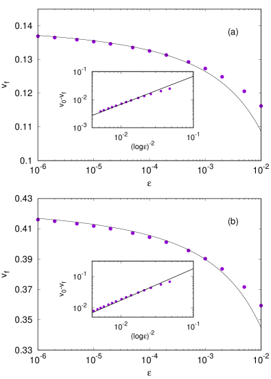
Figure 1: (Color online) Front speed $v_{f}$ vs the cutoff value $\epsilon$ for the RCE with $\tau=1/2$, $u=1$ and (a) $r=0.01$ and (b) $r=0.1$. The solid black curves show the theoretical prediction (14). In particular, the constant $A=v^{\prime\prime}(\lambda_{0})(\pi^{2}\lambda_{0}^{2}/2)$ in front of $(\log\epsilon)^{-2}$ takes the values $A=0.68$ and $1.72$ for $r=0.01$ and $r=0.1$, respectively. The insets show the same data plotting $v_{0}-v_{f}$ against $(\log\epsilon)^{-2}$ to highlight the logarithmic correction, the solid lines are again the theoretical predictions.

Conversely, when $a=r\tau>1$, the approach of Ref. Brunet and Derrida (1997) cannot be used as the linearized treatment becomes meaningless. However, heuristically we can expect that since in this limit the front evolves ballistically the velocity becomes independent of the cutoff and equal to the maximal allowed velocity $v_{f}=u$. Figure 2 displays the numerically observed behavior of the front speed as a function of time for the RCE with different values of the cutoff $\epsilon$, when $a=r\tau=2$.

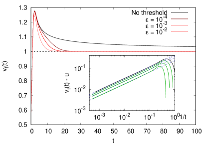
Figure 2: (Color online) Instantaneous front speed $v_{f}(t)$, as defined in main text, vs time for the RCE with $\tau=u=1$, $r=2$ and four different values of the cutoff. The dashed horizontal line stands for the ballistic speed $u=1$. The inset shows $v_{f}(t)-u$ vs $1/t$, to illustrate the trend toward the ballistic speed in the absence of cutoff (from top to bottom $a=r\tau=2.00,1.75,1.50,1.25$). The top black curve corresponds to that of the main panel. The dashed lines display the power law behavior $t^{-0.55}$. Deviations from the behavior $t^{-0.55}$ are observed for $a=r\tau\sim 1$ (not shown).

As one can see, at long times the front speed approaches the asymptotic speed $u$ independently of the value of the cutoff. It is worth noting that the asymptotic speed is approached from greater values. Moreover, while with the cutoff the limiting value $v_{f}=u$ is reached rather quickly, in its absence the convergence is rather slow. Indeed, as shown in the inset of Fig. 2, we found approximately $v_{f}(t)-u\sim t^{-0.55}$ for $a=r\tau$ sufficiently large. This behavior is quite different from what happens in the FKPP case, in which one has, at leading order, $v_{f}(t)-u\sim-t^{-1}$ Van Saarloos (2003); Berestycki et al. (2018). At present we have no explanation for the value $0.55$ of the exponent. This may deserve further investigation but it goes beyond the scope of the present work.

We conclude this section providing some details on the numerical integration of the RCE. In order to have a stable and robust numerical scheme we transformed the original RCE in a system of two first order partial differential equations whose dynamics follow the characteristic functions of the linear wave equation associated to the RCE Aregba-Driollet et al. (2016). Then we used a Roe’s first-order upwind scheme Roe (1987) for the numerical integration of the PDE system. As for the initial condition, we have chosen it to be localized around the center of the system. We measured the instantaneous front speed as $v_{f}(t)=\frac{1}{2}\partial_{t}\int_{0}^{L}n(x,t){\mathrm{d}}x$, which provides an estimate of the bulk reaction speed Constantin et al. (2000). The factor $1/2$ is due to the front propagating in both directions. The limiting speed is obtained by extrapolating the behavior of $v_{f}(t)$ for long times. The simulation stops whenever $n(0,t)$ or $n(L,t)$ is different from zero to avoid boundary effects.

IV Effects of demographic stochasticity

In this section we consider the stochastic individual-based model introduced in Section II in order to study how changes in the carrying capacity, and thus the fluctuations of the number of individuals, influence the front speed, having as a guiding line the results obtained in the continuum limit (Sec. III).

Before starting with the analysis, a comment about the definition of the front speed in the discrete case is in order. A first and natural definition can be given in terms of the growth rate of the total number of particles in the systems $N_{T}(t)$ that, within our model, corresponds to the sum of the number of particles in all the bins in which the domain is discretized, i.e. $N_{T}(t)=\sum_{i=1}^{L/R}n_{i}(t)$. By analogy with the definition of the front speed given at the end of the previous section in the case of a continuous system Constantin et al. (2000), we can define the instantaneous front speed as

$$v^{b}_{f}(t)=\frac{1}{2N}\frac{dN_{T}(t)}{dt}\,,$$ (15)

which expresses the velocity as a bulk property. The word bulk refers to the fact that due to the space average we capture only the large scale properties referring to the whole particle system. The factor $1/2$ accounts again for the fact that propagation occurs in both directions and we recall that $N=N_{p}/R$ is the density of carrying capacity, where $R$ is the bin size and $N_{p}$ is the carrying capacity in a bin.

However, it is also possible to define the front speed in terms of the positions of the extremal particles. Denoting with $x_{m/M}(t)$ the position of the left/rightmost particle, we can define the extremal velocity as

$$v_{f}^{e}(t)=\frac{x_{M}(t)-x_{m}(t)}{2t}\,.$$ (16)

This definition does not probe a bulk property of the traveling front but only concerns the behavior of its edges. In both cases, the asymptotic (long time) front speed, which is the quantity we are interested in, can be obtained extrapolating the constant behavior in the limit of long times, i.e. $v_{f}=\lim_{t\to\infty}v_{f}(t)$. Numerically this is done by means of a linear fit of the long time behavior of $N_{T}(t)/(2N)$ and $(x_{M}(t)-x_{m}(t))/2$, respectively. As we will see the two definitions may not always lead to the same asymptotic front speed. The above result is at odds with the continuous case, where the bulk and extremal speeds always coincide. In that case the former is defined as at the end of the previous section, while the latter can be defined by introducing a threshold value on the particle density.

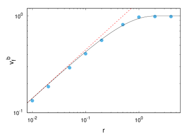
Figure 3: (Color online) Bulk front speed $v^{b}_{f}$ vs $r$ for the stochastic particle model with $N_{p}=100$ and $u=1$, compared with Eq. (13) (solid line) and the FKPP front speed $v_{f}^{{}^{\mathrm{FKPP}}}\!\!=2\sqrt{rD}$ (dashed line).

Let us now discuss the main numerical results. First of all, we measured the asymptotic front speed upon fixing the carrying capacity and varying the reaction rate $r$, to test whether the continuum-limit prediction (13) catches the behavior of the individual-based model. In Figure 3 we show the bulk front speed, $v^{b}_{f}$, obtained using the definition (15) (indistinguishable results are obtained using Eq. (16)). As one can see, Eq. (13) well captures the behavior of $v^{b}_{f}$, confirming that the RCE indeed provides the continuum limit of the system under consideration. The front speed of the FKPP model also appears to be a good approximation for $r\tau\ll 1$ (see the dashed line in the plot). However, small deviations (here hidden by the scale of the graph) are present. These are due to the fluctuations of the number of individuals that are unavoidable in the discrete case. In the following we study in detail how such fluctuations affect the front speed. Knowing from the study of the RCE with a cutoff that the two regimes $r\tau<1$ and $r\tau>1$ are different we will discuss them separately.

IV.1 Low reaction rates

For low reaction rates, $r\tau<1$, as discussed in Sec. III, the RCE behaves essentially as a standard RD system and the effect of a cutoff, $\epsilon$, on the reaction is well described by the results of Brunet and Derrida Brunet and Derrida (1997) (see Fig. 1), originally derived for FKPP-like dynamics. Hence, we should expect that changing the carrying capacity in the stochastic model should have an effect similar to that of varying the cutoff in the RCE and, thus, that the front speed should behave according to the prediction (14) with $\epsilon\sim 1/N=R/N_{p}$. This is confirmed in Fig. 4 that shows the bulk front speed, $v^{b}_{f}$, as a function of $1/N$ for the same reaction rates as those chosen for the RCE (Fig. 1). The prediction (14) is quantitatively well verified but for a small difference in the value of the $N\to\infty$ velocity, indeed the fitted value of the velocity differs from the theoretical value (13) by $4\%$. Equivalent results are obtained using the extremal velocity (16), at least for large $N$.

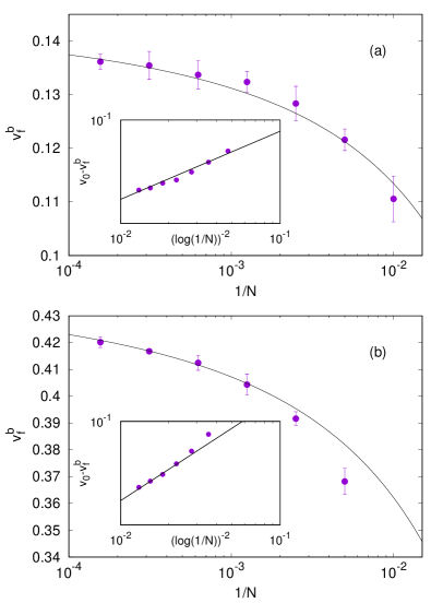
Figure 4: (Color online) Front speed $v^{b}_{f}$ vs $1/N=R/N_{p}$ as obtained from simulations of the stochastic model with $u=1$ and (a) $r=0.01$ and (b) $r=0.1$. The solid curve is obtained by fitting the expression $v^{b}_{f}=v_{0}-A(\log(1/N))^{-2}$ where we fixed $A$ according to Eq. (14) and fitted $v_{0}$; the latter resulted to be $4\%$ higher than the continuum-limit value (13). The insets show the same data plotting $v_{0}-v^{b}_{f}$ against $(\log(1/N))^{-2}$ to highlight the logarithmic correction. We show the average over $10$ simulations with different realizations of the noise, and error bars represent the maximal deviation from the mean.

IV.2 High reaction rates

We now turn to the case $r\tau>1$. In this regime, for the continuous model, the front speed is unaffected by a cutoff in the reaction term (Fig. 2). For the individual-based model, instead, simulations show that the effect of fluctuations on the front speed depends on the definition adopted for $v_{f}$. The bulk speed (15) displays a dependence on the carrying capacity $N_{p}$, while the speed based on the evolution of the front edges (16) is consistent with the results of the continuum limit. The behavior of the latter is shown in Fig. 5, where the time evolution of $v^{e}_{f}(t)$ is shown. The qualitative features are indeed akin to those of Fig. 2: the rightmost and leftmost front edges asymptotically move ballistically into the unoccupied regions ahead of them.

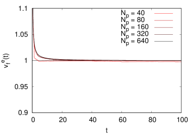
Figure 5: (Color online) Instantaneous front speed $v_{f}^{e}(t)$ as a function of time computed via Eq. (16) for different values of $N_{p}$ for $r=2$ and $u=1$, as obtained by simulation of the stochastic individual-based model. Each curve corresponds to an average over $10$ realizations of the process.

Conversely, as shown in Fig. 6, the bulk front speed, $v_{f}^{b}$, obtained as the long time limit behavior of (15) displays a non-trivial dependence of the front speed on the carrying capacity $N_{p}$. In particular, we found

$$v^{b}_{f}=u\left(1-\frac{C}{N_{p}}\right)$$ (17)

to hold, with a high degree of accuracy for large $N_{p}$.

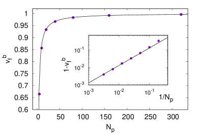
Figure 6: (Color online) Bulk front speed $v^{b}_{f}$ vs $N_{p}$ for $r=4$ and $u=1$ obtained by simulations of the particle model (symbols). The solid curve shows the functional form (17) with $C=1.31$ as obtained by a best fit procedure. The agreement between (17) and the data is very good, as also shown in the inset, where $u-v^{b}_{f}$ is plotted against $1/N_{p}$ for both the numerical data (symbol) and the behavior (17) (solid line).

Clearly we cannot use the continuum theory to explain such a behavior, and the possible explanation must rely on the particle nature of the system, in particular on the stochastic nature of the reaction term that could impact the effective value of the carrying capacity in the bulk. Indeed, at long times the total number of particles is expected to evolve as $N_{T}(t)=2\langle n(N_{p})\rangle v^{e}_{f}t/R$. In other words, at long times $N_{T}$ will be simply the number of invaded bins $2v^{e}_{f}t/R$ (we thus used the definition based on the extremal bins, neglecting the fact that they may have not reached the maximal capacity yet, which is a good approximation at long times) times the average number of individuals in each bin $\langle n(N_{p})\rangle$. Now, using that $v^{e}_{f}=u$ (Fig. 5) we have $N_{T}=2\langle n(N_{p})\rangle ut/R$ that, using (15) and recalling that $N_{p}=NR$, means that the measured bulk velocity will be:

$$v^{b}_{f}=\frac{\langle n(N_{p})\rangle}{N_{p}}u\,.$$ (18)

The above formula would give $v_{f}^{b}=u$ only if $\langle n(N_{p})\rangle=N_{p}$ in the bulk bins. Therefore, the numerical data shown in Fig. 6 provide a strong indication that the expectation $\langle n(N_{p})\rangle=N_{p}$ is violated.

In Appendix B, for stochastic logistic kinetics without transport, we show that the average number of individuals, $\langle n(N_{p})\rangle$, at equilibrium can be computed analytically, see Eq. (35). In particular, when $N_{p}\gg 1$ we have that $\langle n(N_{p})\rangle\approx N_{p}-1$. Plugging this asymptotic expression in (18) yields the heuristic formula (17) with $C=1$, not far from the value $C\approx 1.31$ obtained from a best fit of the numerical data. Clearly, under the action of transport mechanisms the number of particles in the bin will depend not only on the reaction dynamics inside the bin but also on the migration from and toward neighboring bins. Most likely, the fluctuations induced by the transport process are responsible for the deviation of $C$ from $1$.

We conclude this section noticing that similar corrections to the front speed due to the fact that in the bulk $\langle n(N_{p})\rangle\neq N_{p}$ should be present also for $r\tau<1$. However, they are much smaller than the effects discussed in the previous section. Indeed small differences of the bulk velocity from the front speed based on the extremal particles, when $r\tau<1$, can be detected only for small values of $N_{p}$ (not shown), where they are stronger.

V Extension to Levy walks

The model presented in Sec. II can be easily generalized in order to account for more general transport processes, such as Lévy walks Zaburdaev et al. (2015) that can model the transport properties of several biological populations Viswanathan et al. (1999); Bartumeus (2007); Mierke (2013); Ariel et al. (2015), simply modifying the distribution of the walk durations. For instance, with the choice

$$P(T)=(\alpha-1)T^{-\alpha}\Theta(T-1)\,,$$ (19)

at varying the value of $\alpha$ different transport processes can be obtained. Indeed the second moment of the displacement behaves as Andersen et al. (2000):

$$\langle x^{2}(t)\rangle\sim\left\{\begin{array}[]{ll}t^{2}&1<\alpha<2\\ t^{4-\alpha}&2<\alpha<3\\ t&\alpha>3\,,\end{array}\right.$$ (20)

i.e. it is ballistic, superdiffusive or diffusive depending on $\alpha$. Notice that the persistent random walk previously investigated is retrieved in the limit $\alpha\to\infty$. When $\alpha>3$, the diffusive motion stems from the fact that $\langle T^{2}\rangle$ is finite and according to Eq. (2) the diffusion coefficient is equal to

$$D=\frac{u^{2}}{2}\frac{\langle T^{2}\rangle}{\langle T\rangle}=\frac{u^{2}}{2}\frac{\alpha-2}{\alpha-3}\,.$$ (21)

However, even if the diffusion coefficient is well defined for $\alpha>3$, this does not mean that the underlying process is diffusive in a standard way, i.e. it is not true that $\langle x^{2q}\rangle\sim t^{q}$ as expected for a standard diffusive process, see Andersen et al. (2000); Forte et al. (2014) for a discussion. As a consequence, in the case $\alpha<\infty$ the continuum limit of discrete stochastic reactive models, like ours, is nontrivial and can be defined only in the form of an integro-differential equation with a kernel describing the transport process Fedotov (2001, 2016); Stage et al. (2016). However it is still possible to provide an approximate expression for the front speed by appropriately generalizing the results of the previous sections, when the mean square particle displacement has a diffusive behavior (i.e. for $\alpha>3$).

Before discussing this point, let us mention that when $\alpha<3$ it is physically reasonable to expect that $v_{f}\approx u$, besides possible finite $N_{p}$ corrections (Sec. IV.2). This result finds analytical support in Ref. Fedotov (2016) in the strong ballistic case ($\alpha<2$). When the transport process is superdiffusive ($2<\alpha<3$), it should similarly hold, due to the large statistical weight of events characterized by particles keeping their velocity for a very long time. In both cases, tests in numerical simulations of the discrete model confirm the expectation $v_{f}\approx u$ but for finite-$N_{p}$ corrections of the type discussed in Sec. IV.2 (results not shown).

Let us now focus on the range $3<\alpha<\infty$, where the motion is diffusive with diffusion coefficient given by Eq. (21). In this case, the phenomenology of front propagation should not be too different from the one described by the RCE (see Sec. IIIA). In other terms we can conjecture that, when $r$ is sufficiently small, the continuum front speed is given by $v_{0}=2\sqrt{D(\alpha)r}/(1+r\tau(\alpha))$, with $D(\alpha)$ as from Eq. (21) and $\tau(\alpha)=\langle T\rangle/2=(\alpha-1)/[2(\alpha-2)]$, while $v_{f}=u$ for large enough $r$. Hence, substituting the expression of $D(\alpha)$ and rearranging the terms, the front speed should be given by

$$v_{0}=\left\{\begin{array}[]{ll}\frac{2u\sqrt{r\tau}}{1+r\tau}\sqrt{\frac{\langle T^{2}\rangle}{\langle T\rangle^{2}}}&\mathrm{if}\quad r\tau<1\\ u&\mathrm{if}\quad r\tau\geq 1,\end{array}\right.$$ (22)

in close analogy with Eq. (13), apart from a finite $\alpha$ correction controlled by the ratio $\langle T^{2}\rangle/\langle T\rangle^{2}=(\alpha-2)^{2}/[(\alpha-3)(\alpha-1)]$ and the fact that now $\tau$ depends on $\alpha$.

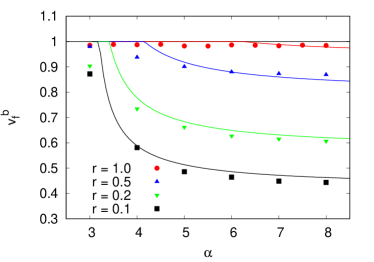
Figure 7: (Color online) Front speed vs $\alpha$ for various values of $r$, with $u=1$ and $N_{p}=100$. Solid lines represent the approximation (22).

To test the validity of prediction (22), we measured the bulk front speed in numerical simulations of the stochastic particle model with the walk-duration probability density function (19) for several values of $\alpha$ and $r$, with $N_{p}=100$ and $u=1$. The results are reported in Fig. 7, where the continuous lines represent the prediction (22). We can first remark that, for any fixed $\alpha$ the front speed tends to the ballistic velocity $u$ with growing $r$ and the convergence is the faster the smaller $\alpha$. As for the dependency on $\alpha$ at fixed $r$, the theoretical prediction describes fairly well the numerical data when $\alpha$ and $r$ are such that $r\tau(\alpha)\ll 1$. The agreement improves as $\alpha$ gets larger, which is reasonable considering that the argument developed above amounts to a correction to the front speed in the RCE (13) due to finite $\alpha$. The more important deviations observed when $\alpha$ approaches 3 are likely due to the increased statistical significance of persistent walks of particularly large duration. Moreover, the case $\alpha=3$ is marginally diffusive as $\langle x^{2}(t)\rangle\sim t\log(t)$. For $\alpha=4$ and $8$ we also studied the dependence of the front speed on $N_{p}$. We found that the fluctuations induced by demographic stochasticity have effects that are quantitatively similar to those discussed in the case of the persistent random walk for low (Sec. IV.1) and high (Sec. IV.2) reaction rates (results not shown). However, it is worth mentioning that for smaller values of $\alpha$ the probability of walks lasting for a long time increases and the assessment of the effects of discreteness becomes more difficult, as longer simulations as well as averages over a larger number of realizations are needed to safely estimate the front speed.

VI Conclusions

We investigated the dynamics of a system of logistically reacting individuals that move according to a one-dimensional persistent random walk, focusing on front propagation and the effect of finite-population fluctuations on it. Such a description of the transport process allows to remedy the unphysical features (such as infinite velocities) of the standard diffusive approximation, which cause an overestimate of the speed of traveling waves.

After deriving the continuum limit of the individual-based model, which corresponds to the RCE, in order to study the effects of discreteness, we introduced a low-population-density cutoff in the reaction term of the continuous-model equation. This allowed us to quantify the correction to the front speed due to the finite number of particles. For low reaction rates ($r\tau<1$) it has been possible to analytically compute it by generalizing the treatment previously introduced for the FKPP model Brunet and Derrida (1997). Similarly to that case, we found that the correction is logarithmic with the density of carrying capacity $N$, $v_{0}-v_{f}\sim(\log(1/N))^{-2}$ (with $v_{0}$ the value from the continuum theory), in good agreement with the results of numerical simulations of the discrete model. For high reaction rates ($r\tau>1$), instead, the numerics indicate that the RCE is insensitive to the cutoff. However, demographic stochasticity does impact the particle dynamics. This result is subtle and tightly related to the definition of the front speed. When the latter is computed from the position of the farthest particle from the origin, the results of the continuum are reproduced. Nevertheless, when $v_{f}$ is computed from the growth rate of the total number of particles, our numerical calculations indicate that $u-v_{f}\sim N_{p}^{-1}$, where $N_{p}$ is the local carrying capacity. Such a reduction of the front speed (with respect to the ballistic velocity) hence originates from the effect of the stochastic nature of the dynamics on the bulk properties of the system, namely from the reduction of the effective (average) carrying capacity, as also confirmed by a simplified probabilistic model (developed in Appendix B).

While the results for the case $r\tau<1$ share important formal similarities with the analogous ones holding for FKPP dynamics Brunet and Derrida (1997), those obtained for $r\tau>1$ are more original and specific to the RCE, and had not been documented before. It is worth to remark that, from a biological point of view, the latter regime corresponds to a situation in which individuals reproduce faster than the typical time at which they change their direction. According to previous studies Holmes (1993) this condition is difficult to achieve even by selecting organisms with high intrinsic growth rate $r$. Nevertheless, we believe that it might still be of importance in the case of fast reproducing (parasites or pathogens) species that, similarly to the spreading by long-range dispersal considered in Hallatshcek and Fisher (2014), are transported by other organisms, characterized by a highly correlated motion.

Finally, we provided an extension of the above picture for power-law distributed walk durations, as is the case when transport is governed by a Lévy walk process relevant to several biological populations Viswanathan et al. (1999); Bartumeus (2007); Mierke (2013); Ariel et al. (2015). In particular, in the diffusive regime ($\alpha>3$), we have shown that the front speed of reaction fronts is well predicted by the RCE with the appropriate diffusion coefficient, at least for not too small values of $\alpha$, and we determined the $\alpha-$dependent correction to the asymptotic front speed in the low-reaction-rate limit.

The predictions obtained in this work concern measurable quantities, such as the front speed and the carrying capacity. Therefore they can be usefully compared to experimental data. We hope that they can stimulate experimental researches and contribute to the understanding of the complex dynamics of biological and chemical reactive species in realistic situations, where correlated movements represent an unavoidable feature.

Appendix A Calculation of the front speed for the RCE with a small cutoff

We consider here the RCE (9) with a cutoff $\epsilon$ in the reaction term, i.e. $f(n)$ is replaced by $f(n)\Theta(n-\epsilon)$, $\Theta$ being the Heaviside step function. Following Ref. Brunet and Derrida (1997) we compute the corrections to the front speed due to the cutoff, obtaining Eq. (14) for the RCE.

Assuming $n(x,t)=h(x-v_{\epsilon}t)=h(z)$, Eq. (9) takes the form

$$(1\!-\!av_{\epsilon}^{2})h^{\prime\prime}\!+\!v_{\epsilon}[1\!-\!af^{\prime}(h)\Theta(n\!-\!\epsilon)]\!+\!f(h)\Theta(n\!-\!\epsilon)\!=\!0\,,$$ (23)

with $f(h)=h(1-h)$. For $\epsilon\ll 1$ we can identify three regions: (I) $\epsilon\ll h\ll 1$, where the cutoff has no influence on the front; (II) $\epsilon\lesssim h\ll 1$, where the cutoff effects are important; $h<\epsilon$ where the reaction is absent.

In region (I) the front, being unaffected by the cutoff, for large $z$ and small $h$, will be of the form:

$$h_{I}(z)\approx Aze^{-\lambda_{0}z}\,,$$ (24)

with $\lambda_{0}$ as in (12). Indeed for $\lambda=\lambda_{0}$ the dispersion relation (11) attains its minimum where $\lambda_{0}$ is a degenerate root of the characteristic equation. In regions (II) and (III), Eq. (23) can be linearized as

$$(1-av_{\epsilon}^{2})h_{II\phantom{I}}^{\prime\prime} + v_{\epsilon}(1-a)h^{\prime}_{II}+h_{II}=0\,,$$ (25)

$$(1-av_{\epsilon}^{2})h_{III}^{\prime\prime} + v_{\epsilon}h^{\prime}_{III}=0\,.$$ (26)

Equation (25) is the same as Eq. (10), and can be solved similarly by assuming $h_{II}(z)\propto e^{-\lambda_{\epsilon}z}$. However, here we have an effect of the cutoff $\epsilon$, i.e. the $\lambda_{\epsilon}$ solving the characteristic equation depends on $\epsilon$. Denoting with $0<\Delta\ll 1$ the difference $v_{0}-v_{\epsilon}$, since $v_{0}$ corresponds to the minimum of the dispersion relation (11) we have that

$$v_{\epsilon}-v_{0}=-\Delta\approx(1/2)v^{\prime\prime}(\lambda_{0})(\lambda_{\epsilon}-\lambda_{0})^{2}\,,$$ (27)

implying that we have two complex conjugate roots, i.e. $\lambda_{\epsilon}=\lambda_{\epsilon}^{r}\pm i\lambda_{\epsilon}^{i}$, and from (27) clearly we have $\lambda_{\epsilon}^{i}\sim\Delta^{1/2}$ while $\lambda_{\epsilon}^{r}\approx\lambda_{0}$. Since we now have two complex conjugate roots, Eq. (25) is solved by

$$h_{II}(z)\approx Ce^{-\lambda^{r}_{\epsilon}z}\sin(\lambda_{\epsilon}^{i}z+D)\,.$$ (28)

Equation (26) instead has the solution

$$h_{III}(z)=\epsilon\exp[-v_{\epsilon}(z-z_{0})/(1-av_{\epsilon})]\,,$$ (29)

the front reaching the cutoff value at $z_{0}$.

Thus we end up with four unknowns: $C,D,z_{0}$ and $v_{\epsilon}$ (assuming $A$ as given from the unperturbed dynamics), which have to be fixed imposing the continuity of $h$ and of its derivative at the borders between regions I/II and II/III. It is easy to see that to match the functions (24) and (28), one must require $D=0$ so that, thanks to the fact that $\lambda_{\epsilon}^{i}\sim\Delta^{1/2}\ll 1$, by expanding the sine and to leading order in $\Delta^{1/2}$ we have $C=A/\lambda_{\epsilon}^{i}$. Then, by imposing the continuity of (28) and (29) and of their derivatives at $z_{0}$ we obtain the two relations:

$$Ae^{-\lambda_{\epsilon}^{r}z_{0}}\sin(\lambda_{\epsilon}^{i}z_{0}) = \epsilon\lambda_{\epsilon}^{i}$$ (30)

$$Ae^{-\lambda_{\epsilon}^{r}z_{0}}(-\lambda_{\epsilon}^{r}\sin(\lambda_{\epsilon}^{i}z_{0})+\lambda_{\epsilon}^{i}\cos(\lambda_{\epsilon}^{i}z_{0})) = -\epsilon\lambda_{\epsilon}^{i}\frac{v_{\epsilon}}{(1-av_{\epsilon}^{2})}\,.$$

Dividing the second by the first yields

$$-\lambda_{\epsilon}^{r}+\frac{\lambda_{\epsilon}^{i}}{\tan(\lambda_{\epsilon}^{i}z_{0})}=-\frac{v_{\epsilon}}{1-av_{\epsilon}^{2}}\,,$$ (31)

which is similar but not identical to that obtained by Brunet and Derrida (1997). In order to fix the value of $z_{0}$ using the above expression we recall that $\lambda_{\epsilon}^{i}\sim\Delta^{1/2}$ and $\lambda_{\epsilon}^{r}\approx\lambda_{0}$, and to the same order $v_{\epsilon}\approx v_{0}$. Substituting these approximations in (31) and using Eq. (12), after simple algebra one obtains ${\lambda_{\epsilon}^{i}}/{\lambda_{0}^{2}}\approx-\tan(\lambda_{\epsilon}^{i}z_{0})$. The last equation can be solved by assuming $\lambda_{\epsilon}^{i}z_{0}\approx\pi-\beta$ with $\beta\ll 1$ and Taylor expanding the tangent which gives $\beta=\lambda_{\epsilon}^{i}/\lambda_{0}^{2}\propto\Delta^{1/2}$, consistently with the assumption of a small quantity. Substituting $\lambda_{\epsilon}^{i}z_{0}\approx\pi-\beta$ in the argument of the sine in the first of (30), Taylor expanding and solving for $z_{0}$ we obtain to leading order for $\epsilon\ll 1$: $z_{0}\approx-\log(\epsilon\lambda_{0}^{2})/\lambda_{0}\approx-\log\epsilon/\lambda_{0}$. Then, to order $\Delta^{1/2}$, we have $\lambda_{\epsilon}^{i}\approx\pi/z_{0}\approx-\pi\lambda_{0}/\log\epsilon$. Finally, using the above results, the fact that $\lambda_{\epsilon}-\lambda_{0}\approx i\lambda_{\epsilon}^{i}$ and Eq. (27) we obtain the result (14) of Sec. III.2, which was the goal of this Appendix.

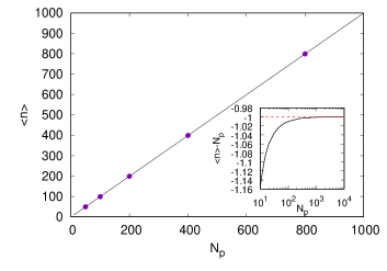
Figure 8: Average number of individuals $\langle n\rangle$ vs $N_{p}$ as computed by simulations, based on a standard Gillespie algorithm Gillespie (1977), of the non-spatial stochastic logistic model (symbols) and corresponding exact solution (35) (solid line), obtained from Mathematica. The inset shows the analytical curve $\langle n\rangle-N_{p}$ and how it converges to $-1$, which justifies Eq. (36).

Appendix B Exact solution of the stochastic logistic equation

In this section we consider the discrete logistic dynamics in the absence of transport. The number of individuals at time $t$, $n(t)$, evolves according to the kinetics (3-5), i.e. it increases (decreases) by one with a rate $W^{+}(n)=rn$ respectively $W^{-}(n)=rn^{2}/N_{p}$, $N_{p}$ denoting the carrying capacity). Thus the probability to have $n$ individuals at time $t$ evolves according to the master equation,

$$\partial_{t}P_{t}(n) = W^{+}(n-1)P_{t}(n-1)+W^{-}(n+1)P_{t}(n+1)$$ (32)

$$- (W^{+}(n)+W^{-}(n))P_{t}(n)\,.$$

At equilibrium, the detailed balance condition, $P(n\!+\!1)W^{-}(n\!+\!1)\!=\!P(n)W^{+}(n)$ (where $P(n)\!=\!\lim_{t\to\infty}P_{t}(n)$), should hold, so that we can write the recurrence relation $P(n+1)=\frac{nN_{p}}{(n+1)^{2}}P(n)$, which is solved by

$$P(n)=\frac{(N_{p})^{n}}{n\cdot n!}P(1)\,,$$ (33)

where $P(1)$ can be fixed using the normalization condition, $\sum_{n=1}^{\infty}P(n)=1$. Using Mathematica we obtained

$$\frac{1}{P(1)}=\sum_{n=1}^{\infty}\frac{(N_{p})^{n}}{n\cdot n!}=-\gamma-\Gamma(0,-N_{p})-\log(-N_{p})\,,$$ (34)

where $\gamma$ is Euler-Mascheroni constant, and $\Gamma(0,-N_{p})$ is the upper incomplete Gamma function. Once we have the expression for $P(n)$ we can compute the average number of individuals, $\langle n\rangle$, at stationarity as

$$\langle n\rangle=\sum_{n=1}^{\infty}nP(n)=(e^{N_{p}}-1)P(1)$$ (35)

which asymptotically reaches $N_{p}$, but the correction for large $N_{p}$ goes as follows (see also Fig. 8)

$$\langle n\rangle\approx{N_{p}-1}\,.$$ (36)

References

- Clavin (1994) P. Clavin, “Premixed combustion and gasdynamics,” Annu. Rev. Fluid Mech. 26, 321–352 (1994).
- Fisher (1937) R. A. Fisher, “The wave of advance of advantageous genes,” Ann. Eugenics 7, 355–369 (1937).
- Aronson and Weinberger (1975) D. G. Aronson and H. F. Weinberger, “Nonlinear diffusion in population genetics, combustion, and nerve pulse propagation,” in Partial differential equations and related topics (Springer, 1975) pp. 5–49.
- Korolev et al. (2010) K. S. Korolev, M. Avlund, O. Hallatschek, and D. R. Nelson, “Genetic demixing and evolution in linear stepping stone models,” Rev. Mod. Phys. 82, 1691 (2010).
- Murray (2002) J. D. Murray, Mathematical Biology 1: An Introduction, 3rd ed. (Springer, 2002).
- Okubo and Levin (2001) A. Okubo and S. A. Levin, Diffusion and ecological problems: modern perspectives (Springer, 2001).
- Skellam (1951) J. G. Skellam, “Random dispersal in theoretical populations,” Biometrika 38, 196–218 (1951).
- Stinner et al. (1983) R. E. Stinner, C. S. Barfield, J. L. Stimac, and L. Dohse, “Dispersal and movement of insect pests,” Ann. Rev. Entomol. 28, 319–335 (1983).
- Turchin (1989) P. Turchin, “Beyond simple diffusion: models of not-so-simple movement in animals and cells,” Comm. Theor. Biol. 1, 65–83 (1989).
- Holmes (1993) E. E. Holmes, “Are diffusion models too simple? a comparison with telegraph models of invasion,” Amer. Natur. 142, 779–795 (1993).
- Codling et al. (2008) E. A. Codling, M. J. Plank, and S. Benhamou, “Random walk models in biology,” J. R. Soc. Interface 5, 813–834 (2008).
- Garcia et al. (2011) M. Garcia, S. Berti, P. Peyla, and S. Rafaï, “Random walk of a swimmer in a low-Reynolds-number medium,” Phys. Rev. E 83, 035301(R) (2011).
- Méndez et al. (2013) V. Méndez, D. Campos, and F. Bartumeus, Stochastic foundations in movement ecology (Springer, New York, 2013) pp. 177–205.
- Hadeler (1994) K.P. Hadeler, “Travelling fronts for correlated random walks,” Canad. Appl. Math. Quart 2, 27–43 (1994).
- Lemarchand and Nawakowski (1998) A. Lemarchand and B. Nawakowski, “Perturbation of local equilibrium by a chemical wave front,” J. Chem. Phys. 109, 7028–7037 (1998).
- Horsthemke (1999) W. Horsthemke, “Fisher waves in reaction random walks,” Phys. Lett. A 263, 285–292 (1999).
- Galenko and Danilov (2000) P. K. Galenko and D. A. Danilov, “Hyperbolic self-consistent problem of heat transfer in rapid solidification of supercooled liquid,” Phys. Lett. A 278, 129–138 (2000).
- Fort and Méndez (2002a) J. Fort and V. Méndez, “Wavefronts in time-delayed reaction-diffusion systems. Theory and comparison to experiment,” Rep. Progr. Phys. 65, 895 (2002a).
- Fort and Méndez (2002b) J. Fort and V. Méndez, “Time-delayed spread of viruses in growing plaques,” Phys. Rev. Lett. 89, 178101 (2002b).
- Fort (2003) J. Fort, “Population expansion in the western pacific (austronesia): A wave of advance model,” Antiquity 77, 520–530 (2003).
- Durrett and Levin (1994) R. Durrett and S. Levin, “The importance of being discrete (and spatial),” Theor. Pop. Biol. 46, 363–394 (1994).
- Zaburdaev et al. (2015) V Zaburdaev, S Denisov, and J Klafter, “Lévy walks,” Rev. Mod. Phys. 87, 483 (2015).
- Van Saarloos (2003) W. Van Saarloos, “Front propagation into unstable states,” Phys. Rep. 386, 29–222 (2003).
- Kolmogorov et al. (1937) A. Kolmogorov, I. Petrovskii, and N Piskunov, “Study of a diffusion equation that is related to the growth of a quality of matter and its application to a biological problem,” Bull. Univ. Moscow 1, 1 (1937).
- Brunet and Derrida (1997) E. Brunet and B. Derrida, “Shift in the velocity of a front due to a cutoff,” Phys. Rev. E 56, 2597 (1997).
- Patlak (1953) C. S. Patlak, “Random walk with persistence and external bias,” Bull. Math. Biophys. 15, 311–338 (1953).
- Forte et al. (2014) G. Forte, F. Cecconi, and A. Vulpiani, “Non-anomalous diffusion is not always Gaussian,” Europ. Phys. J. B 87, 102 (2014).
- Pigolotti et al. (2012) S. Pigolotti, R. Benzi, Mogens H. Jensen, and D. R. Nelson, “Population genetics in compressible flows,” Phys. Rev. Lett. 108, 128102 (2012).
- Perlekar et al. (2011) P. Perlekar, R. Benzi, S. Pigolotti, and F. Toschi, “Particle algorithms for population dynamics in flows,” J. Phys.: Conf. Ser. 333, 012013 (2011).
- Note (1) If corresponds to the th bin, i.e. , is defined by in the limit .
- Cencini et al. (2003) M. Cencini, C. Lopez, and D. Vergni, “Reaction-diffusion systems: front propagation and spatial structures,” in The Kolmogorov Legacy in Physics, Lecture Notes in Physics, Vol. 636 (Springer, 2003) pp. 187–210.
- Berestycki et al. (2018) J. Berestycki, E. Brunet, and B. Derrida, “A new approach to computing the asymptotics of the position of Fisher-KPP fronts,” EPL 122, 10001 (2018).
- Aregba-Driollet et al. (2016) D. Aregba-Driollet, M. Briani, and R. Natalini, “Time asymptotic high order schemes for dissipative bgk hyperbolic systems,” Numer. Math. 132, 399–431 (2016).
- Roe (1987) P.L. Roe, “Upwind differencing schemes for hyperbolic conservation laws with source terms,” in Nonlinear hyperbolic problems (Springer, 1987) pp. 41–51.
- Constantin et al. (2000) P. Constantin, A. Kiselev, A. Oberman, and L. Ryzhik, “Bulk burning rate in Passive-Reactive Diffusion,” Arch. Rat. Mech. Anal. 154, 53–91 (2000).
- Viswanathan et al. (1999) G. M. Viswanathan, S. V. Buldyrev, S. Havlin, M. G. E. Da Luz, E. P. Raposo, and H. E. Stanley, “Optimizing the success of random searches,” Nature 401, 911 (1999).
- Bartumeus (2007) F. Bartumeus, “Lévy processes in animal movement: an evolutionary hypothesis,” Fractals 15, 151–162 (2007).
- Mierke (2013) C. T. Mierke, “The integrin alphav beta3 increases cellular stiffness and cytoskeletal remodeling dynamics to facilitate cancer cell invasion,” New J. Phys. 15, 015003 (2013).
- Ariel et al. (2015) G. Ariel, A. Rabani, S. Benisty, J. D. Partridge, R. M. Harshey, and Avraham Be’er, “Swarming bacteria migrate by lévy walk,” Nat. Commu. 6, 8396 (2015).
- Andersen et al. (2000) K.H. Andersen, P. Castiglione, A. Mazzino, and A. Vulpiani, “Simple stochastic models showing strong anomalous diffusion,” Europ. Phys. J. B 18, 447–452 (2000).
- Fedotov (2001) S. Fedotov, “Front propagation into an unstable state of reaction-transport systems,” Phys. Rev. Lett. 86, 926 (2001).
- Fedotov (2016) S. Fedotov, “Single integrodifferential wave equation for a Lévy walk,” Phys. Rev. E 93, 020101 (2016).
- Stage et al. (2016) H. Stage, S. Fedotov, and V. Méndez, “Proliferating Lévy walkers and front propagation,” Math. Mod. Nat. Phenom. 11, 157–178 (2016).
- Hallatshcek and Fisher (2014) O. Hallatshcek and D. S. Fisher, “Acceleration of evolutionary spread by long-range dispersal,” Proc. Natl. Am. Soc. 111, E4911–E4919 (2014).
- Gillespie (1977) D. T Gillespie, “Exact stochastic simulation of coupled chemical reactions,” J. Phys. Chem. 81, 2340–2361 (1977).