Discontinuous shear-thinning in adhesive dispersions

Abstract

We present simulations for the steady-shear rheology of a model adhesive dispersion in the dense regime. We vary the range of the attractive inter-particle forces $u$ as well as the strength of the dissipation $b$. For large dissipative forces, the rheology is governed by the Weisenberg number $\text{Wi}\sim b\dot{\gamma}/u$ and displays Herschel-Bulkley form $\sigma=\sigma_{y}+c\text{Wi}^{\nu}$ with exponent $\nu=0.45$. Decreasing the strength of dissipation, the scaling with Wi breaks down and inertial effects show up. The stress decreases via the Johnson-Samwer law $\Delta\sigma\sim T_{s}^{2/3}$, where temperature $T_{s}$ is exclusively due to shear-induced vibrations. During flow particles prefer to rotate around each other such that the dominant velocities are directed tangentially to the particle surfaces. This tangential channel of energy dissipation and its suppression leads to a discontinuity in the flow curve, and an associated discontinuous shear thinning transition. We set up an analogy with frictional systems, where the phenomenon of discontinuous shear thickening occurs. In both cases, tangential forces, frictional or viscous, mediate a transition from one branch of the flowcurve with low tangential dissipation to one with larger tangential dissipation.

I Introduction

Dense dispersions, like colloids or emulsions, display a broad range of different rheological properties. This variety mirrors the action of the different forces acting on and between the particles making the dispersion. In general, it is not at all clear which of these forces or combinations are relevant for a particular phenomenon on the continuum level. Still, identification of the relevant players is needed for a proper design of new materials, which has become increasingly important in different industrial settings, like food or cosmetics Laba (1993). Using simulations, simplified model systems can be defined to close this gap in understanding. By tuning the interaction forces dominant parameter dependencies can be isolated and the underlying physical mechanisms identified.

In this contribution, we are interested in the role of different dissipative forces on flowing adhesive dispersions. The attractive inter-particle forces in dispersions may be due to various mechanisms, e.g. depletion forces Bécu et al. (2006); Ballesta et al. (2013) or direct interactions Blijdenstein et al. (2004). In the case of granular materials, attraction can appear e.g. via the development of capillary bridges Hornbaker D. J. et al. (1997); Herminghaus (2005); Mitarai and Nori (2006). At rest, attractive forces quite generally assist in the formation of clusters or gel-like networks Kim and Mason (2017). In the flowing state Eberle et al. (2014); Bounoua and Lemaire (2016) there is then a continuous competition between the rupturing of the network and aggregation processes that try to restore local structure Martens et al. (2012); Coussot (2007).

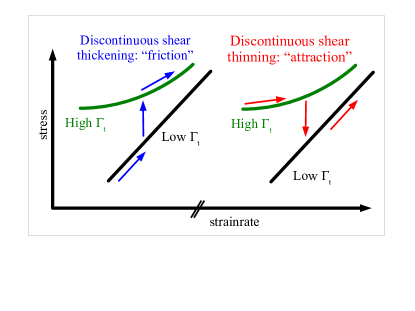
Figure 1: Schematic flowcurves, comparing the two phenomena of discontinuous shear-thickening and discontinuous shear-thinning. Both are mediated by the presence of a “tangential” channel of energy dissipation (dissipation is due to sliding velocities directed tangentially to particle surfaces). Shear thickening is due to a rapid increase of frictional dissipation $\Gamma_{t}$ upon increasing strainrate. On the other hand, shear thinning in the adhesive system studied here occurs because tangential viscous interactions are only relevant in dense gel-like structures, which are broken down upon increasing the strainrate.

Dissipation in emulsions and suspensions is primarily of hydrodynamic origin, e.g., in the form of lubrication forces or long-range hydrodynamic interactions. In granular powders, inelastic collisions and dry friction dominate the dissipation. In wet granular media, finally, the breaking of liquid capillary bridges between near by particles is important Strauch and Herminghaus (2012). Many of these forces also have a directional dependence. Lubrication, for example, has a squeeze and a shear-mode, the latter often thought to be negligible as to its logarithmic gap-dependence Kim and Karrila (2005). In highly dense suspensions, close to jamming, it is becoming clear, however, that shear forces – acting tangentially to the particle surface – may fundamentally affect the emerging rheology. Baumgarten et al.  Baumgarten and Tighe (2017) have argued that tangential viscous interactions, even if they are small, are necessary to obtain dynamic critical scaling for the linear visco-elasticity of jammed systems. Similarly, Vagberg et al. Vågberg et al. (2017) demonstrate the key role that this tangential dissipation plays for the small-strainrate rheology. In a different system, solid-solid friction between particles leads to shear-thickening where the associated frictionless system would only display shear-thinning Heussinger (2013). In particular, this friction-induced shear-thickening has received a lot of attention recently Clavaud et al. (2017); Saint-Michel et al. (2018); Wyart and Cates (2014); Grob et al. (2016). The relevant tangential forces in this scenario may even be strong enough to lead to a discontinuous jump of the stress over several orders of magnitude, or to a sudden arrest upon increasing the strainrate Grob et al. (2014); Seto et al. (2013). In the granular community, the combination of frictional interactions with cohesive forces has been studied in a variety of contexts, e.g. in Refs. Singh et al. (2014); Gu et al. (2014); Gilabert et al. (2007); Berger et al. (2015); Khamseh et al. (2015); Rognon et al. (2008)

In this work, using numerical simulations, we investigate the influence of a tangential viscous force on the steady-state flow behavior of dense assemblies of adhesive (but non-frictional) particles. The important finding is that the presence of this additional mode of dissipation gives rise to a discontinuity in the flow-curves, in the under-damped limit, quite similar to the phenomenon of discontinuous shear-thickening observed in frictional systems. In both cases, tangential forces, frictional or viscous, mediate a transition from one branch of the flowcurve with low tangential dissipation $\Gamma_{t}$ to one with large $\Gamma_{t}$ (see Fig. 1). Furthermore, such discontinuities in the flow curve leads to formation of shear-bands, with contrasting flow rates and local packing, providing yet another scenario where persistent flow heterogeneities can happen.

II Model

We consider a two-dimensional system of $N$ soft disks interacting via the following potential:

$$V(r_{ij})=\begin{cases}\epsilon\left[(1-\frac{r_{ij}}{d_{ij}})^{2}-2u^{2}\right],&\frac{r_{ij}}{d_{ij}}<1+u\\ -\epsilon\left[1+2u-\frac{r_{ij}}{d_{ij}}\right]^{2},&1+u<\frac{r_{ij}}{d_{ij}}<1+2u\\ 0,&\frac{r_{ij}}{d_{ij}}>1+2u\\ \end{cases}$$ (1)

where $r_{ij}=|\vec{r}_{i}-\vec{r}_{j}|$ is the distance between the $i$th and $j$th particles, and $d_{ij}=(d_{i}+d_{j})/2$ is the average of their diameters. Thus, there exists a harmonic repulsive interaction when the particles overlap, $r_{ij}<d_{ij}$. Additionally, there is a short-range attractive interaction between the particles when the distance is within some threshold, $d_{ij}<r_{ij}<d_{ij}(1+2u)$. The parameter $u$ is introduced to characterize the width ($2u$) and also the strength ($\epsilon u^{2}$) of the attractive potential. The scale for attractive forces is then $\epsilon u/d$. Thus, attractive forces are characterized by a single parameter. This greatly reduces the computational complexity and at the same time keeps the model as simple as possible. In general, we will consider only the case where the range of attraction is very small as compared to the particle size. This sets our model apart from LJ-like models, where attraction usually ranges beyond the first neighbor shell.

In addition to the conservative force, a dissipative force acts between pairs of particles. This viscous force is proportional to their relative velocity and acts only when particles overlap, i.e. $r_{ij}<d_{ij}$,

$$\vec{F}_{\text{diss.}}=-b[\vec{v}_{i}-\vec{v}_{j}]$$ (2)

where $b$ is the damping coefficient. In this model, which is equivalent to the model coined CD in Ref. Vågberg et al. (2014), particle rotations are not accounted for. As discussed in that reference, rotations are decoupled from the translational degrees of freedom and therefore can be dropped. It should be noted, that this is different from the standard Cundall-Strack model Cundall and Strack (1079) for solid friction between particles. In that model, the dissipative force is taken as the relative velocity at the contact, which also involves rotations. Here, it is the relative center-of-mass velocity, which enters the dissipative force law, Eq. (2).

The damping force can be split in components normal and tangential to the direction defined by the corresponding contact of the two particles, $\hat{n}_{ij}=(\vec{r}_{i}-\vec{r}_{j})/r_{ij}$. The normal contribution, for example, reads

$$\vec{F}_{\rm diss}^{(n)}=-b[\vec{v}_{ij}\cdot\hat{n}_{ij}]\hat{n}_{ij}\,.$$

In previous work, we have studied the rheological properties in systems with only this normal contribution Irani et al. (2016, 2014). Below we will make frequent comparison with that work.

To investigate the rheology of such a system of particles, we perform molecular dynamics simulations using LAMMPS Plimpton (1995). In order to avoid crystallization, we choose a 50:50 binary mixture of particles having two different sizes, with a relative radii of 1.4. The system is sheared in $\hat{x}$ direction with a strain rate $\dot{\gamma}$ using Lees-Edwards boundary conditions. The volume fraction is $\phi=\sum_{i=1}^{N}\pi(d_{i}/2L)^{2}$, where $L$ is the length of the simulation box.

The unit of energy is $\epsilon$ and the unit of length is the diameter of the smaller particle type, $d=1.0$. The unit of time is hence $d/\sqrt{\epsilon/m}$, where $m=1.0$ is the mass of the particles. We use $\delta t=0.005$, as timestep for the integration.

III Results and Discussion

For a given imposed strainrate $\dot{\gamma}$ we measure the shear stress $\sigma$ with the help of the virial expression. The resulting flowcurves $\sigma(\dot{\gamma})$ are displayed in Fig. 2(a) for different damping parameters $b$ at $\phi=0.75$. The corresponding viscosity, $\eta(\dot{\gamma})$, is shown in Fig. 2(b).

The divergent viscosity for vanishing strainrates indicates the presence of a yield-stress. For finite strainrates, decreasing the damping parameter $b$ implements a transition from an overdamped to an underdamped regime. In the overdamped regime ($b\geq 0.5$), as the shear-rate is increased, a viscous Newtonian flow regime, $\sigma\propto\dot{\gamma}$, is encountered, in the intermediate $\dot{\gamma}$ range (dashed line). This translates to a constant viscosity, before the shear-thinning regime at larger shear-rates. For the underdamped regime, the situation is very different. At larger shear-rates, the stress is $\sigma\propto\dot{\gamma}^{2}$ (solid line), which is called Bagnold regime, wherein the viscosity also increases linearly with shear-rate. Note the opposite dependence on $b$ in the two branches. In the viscous branch, the stress decreases with decreasing damping, while in the case of the Bagnold branch, it increases. The latter happens due to the higher velocities in weakly damped systems.

Recent experiments Fall et al. (2010) evidence a simple continuous transition from viscous to Bagnold scaling. The scenario encountered here is seemingly more complex and even involves discontinuous jumps in the stress and consequently the viscosity; see Fig. 2.

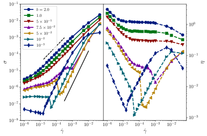
Figure 2: (left) Flow curves (stress $\sigma$ vs shear-rate $\dot{\gamma}$), for $u=2\times 10^{-5}$ and $\phi=0.75$. As $b$ changes, the system crosses from the over-damped to under-damped regime. Solid and dashed lines represent respectivly $\dot{\gamma}^{2}$ and $\dot{\gamma}^{1}$. (right) Corresponding data for viscosity, $\eta(\dot{\gamma})$.

III.0.1 Overdamped systems

In order to understand these unusual features we start by discussing the overdamped limit, where the Weissenberg number has to be used to scale the flow curves. The Weissenberg number is defined as the ratio of dissipative to elastic contributions to the stress. In our case the dissipative stress scale is given by $\sigma_{\text{diss}}\sim b\dot{\gamma}$. The elastic stress scale is $\sigma_{\text{el.}}\sim\epsilon u/d$. Thus, the Weissenberg number can be written as

$$\text{Wi}=\frac{d}{\epsilon}\frac{b\dot{\gamma}}{u}.$$ (3)

The flow stress, ie. after removal of the yield stress, has to be a function of only Wi, $\Delta\sigma=\sigma-\sigma_{y}=\epsilon uF(\text{Wi})$. As the yield stress itself is not accessible in our simulations we determine its value so as to enforce this data collapse. Fig. 3 displays this collapse for the stress $\Delta\sigma$ in the overdamped regime for two different attraction strengths ($u=2\times 10^{-5}$ and $u=2\times 10^{-4}$)  .

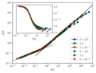
Figure 3: Stress $\Delta\hat{\sigma}=(\sigma-\sigma_{y})/\epsilon u$ vs. Wi of over-damped systems ($b\geq 0.5$) at different attraction ($u$) and damping ($b$) strength. Solid and dashed lines represent, respectively, $u=2\times 10^{-5}$ and $u=2\times 10^{-4}$, with corresponding $\sigma_{y}=1.8\times 10^{-7}$ and $3.4\times 10^{-6}$. The dashed line without symbols displays $\text{Wi}^{\nu}$ ($\nu\approx 0.45$) and the solid line without symbols exhibits $\text{Wi}^{1}$. The inset displays the scaling of corresponding connectivity curves $z$ with the Weissenberg number (Wi).

Apparently, Wi separates two flow regimes, each of which is characterized by a specific exponent $\sigma\sim\text{Wi}^{\nu}$. For high $\text{Wi}>0.3$ the exponent $\nu=1$, thus $\sigma\sim b\dot{\gamma}$ which corresponds to the simple viscous Newtonian regime mentioned above. The attractive forces in this regime are irrelevant.

For low $\text{Wi}<0.3$ the exponent $\nu\approx 0.45$. As we are dealing with a yield-stress fluid this exponent has to be interpreted as a Herschel-Bulkley (HB) exponent. Thus, the expression for the stress becomes

$$\sigma=\sigma_{y}+c\frac{\epsilon u}{d}\text{Wi}^{\nu}\,.$$ (4)

with the yield-stress $\sigma_{y}$ and a constant $c\approx 0.41$. The value of the exponent $\nu$ is in the range observed in other yield-stress fluids (usually between 0.4-0.5), but hardly ever a real power-law regime (straight line in double-logarithmic presentation) is observed. In experiments (and many simulations) only small stress increase over the yield-stress is present.

The yield-stress itself naturally does not scale with the Weisenberg number and is controlled by different physical mechanisms. These mechanisms of flow at the yield stress are by now well understood. Flow comes about as a sequence of elastic branches, during which the solid is elastically strained, and sudden plastic events, at wich this stored energy is released and dissipated Maloney and Lemaître (2006). This gives the stress-strain relation at the yield stress the typical sawtooth apearance Maloney and Lemaître (2006). In the elastic branches the stress increases linearly, $\sigma=g\gamma$, with the slope given by the elastic shear modulus $g$. The plastic events are quasi instantaneous if the strainrate is infinitesimal small. The yield-stress can thus be written in terms of a yield strain $\gamma_{y}$, as $\sigma_{y}=g\gamma_{y}$. In previous work Irani et al. (2016, 2014) we have derived the expressions $g\sim\epsilon\delta\!z_{0}$ and $\gamma_{y}\sim(\delta\!z_{0}u)^{1/2}$, relating both quantities to the connectivity $\delta\!z_{0}=z(\dot{\gamma}=0)-4$. The value $z_{\rm iso}=4$ represents a limiting minimal (isostatic) connectivity that is necessary for a solid (in 2d) to exist. The value of $\delta\!z_{0}$ is generally very small (see inset Fig. 3) indicating the formation of a fragile solid. It is well known that in these near-isostatic systems ($\delta z\to 0$) the linear response to deformation is characterized by strong non-affine motion, with particle displacements that are directed tangentially to particle contacts van Hecke (2010). Thus contacting particles tend to rotate around each other. It is this behavior that leads to the particular scaling of the yield strain $\gamma_{y}$. At finite strainrates displacements translate into velocities, such that the dominant contribution is a relative velocity $v_{ij}^{(t)}$ of two contacting particles ($ij$) in direction tangential (${t}$) to the particle surface. According to the dissipative force law Eq. (2), this motion gives rise to dissipation which shows up in the stress via an energy balance equation

$$\sigma\dot{\gamma}\sim bv^{2}\,.$$ (5)

where the left hand side gives the injected work per unit of time, while the right gives the dissipated power in terms of the mentioned tangential velocities

$$v=\sqrt{\langle v_{ij}^{(t)2}\rangle}\,.$$ (6)

In principle, the velocity component directed normal to the particle surface also has to be accounted for. But, as will be discussed below, this latter contribution is very small in the HB regime and thus can be neglected (see Fig. 6 right).

Rewriting Eq. (5) in terms of Wi and inserting the HB scaling we get

$$v^{2}\sim\dot{\gamma}^{2}\text{Wi}^{\nu-1}$$ (7)

This scaling is tested in Fig. 4.

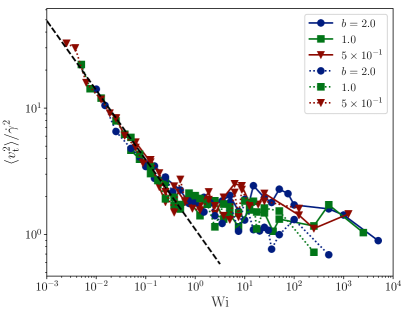
Figure 4: (Particle (tangential) velocities $v^{2}/\dot{\gamma}^{2}$ vs. Wi in the overdamped regime for different attraction ($u$) and damping ($b\geq 0.5$) strength. For small strainrates the velocities scale as $v^{2}\sim\dot{\gamma}^{2}\text{Wi}^{\nu-1}$ with $\nu-1\approx-0.55$ (dashed line). At large strainrates (viscous regime) velocities are nearly independent of Wi and $v\sim\dot{\gamma}$.

III.0.2 Underdamped systems

We now turn to the underdamped regime ($b<0.5$). As is evident from Fig. 2 the flowcurves in this regime acquire a different shape than in the overdamped regime. Furthermore, a discontinuity shows up. The Weisenberg number is therefore no longer sufficient to explain the flow behavior.

To rationalize these findings we follow Nicolas et al. Nicolas et al. (2016) and assume that in underdamped systems enhanced velocities act like a temperature, $T\sim mv^{2}$, that weakens the solid-like structure encountered at small strainrates. Weakening comes about because of activated events that allow plastic rearrangements to take place even though the threshold of the event is not yet reached. As a consequence, the overall stress is lowered by a factor $\Delta\sigma_{\rm therm}$ that we now determine (following Refs. Johnson and Samwer (2005); Chattoraj et al. (2010)).

The energy barrier for a plastic rearrangement at a given strain $\gamma_{c}$ is $\Delta E=k_{B}T_{0}(\gamma-\gamma_{c})^{3/2}$, where $\gamma$ is the currrent strain and $k_{B}T_{0}$ is the overall energy scale of the process Chattoraj et al. (2010). We can take $k_{B}T_{0}\sim\epsilon u^{2}$. Thermal activation is possible, when $\Delta E\approx k_{B}T\sim mv^{2}$. Thus plastic yielding does, in general, not occur at $\gamma_{c}$ (as it would at zero temperature) but at reduced strains $\Delta\gamma\sim(T/T_{0})^{2/3}\sim(v^{2}/u^{2})^{2/3}$. The associated stress reduction is therefore $\Delta\sigma_{\rm therm}=g\Delta\gamma$. The scaling is presented in Fig. 5 . A systematic deviation from the scaling behaviour at small velocities (small strainrates) is due to the lack of precise value for the yield stress. Much longer simulations at lower strainrates would be necessary to overcome this limitation.

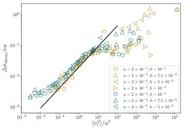
Figure 5: Thermal contribution of the stress $\Delta\sigma_{\rm therm}/\epsilon u$ vs. tangential velocities $v^{2}/u^{2}$. The line corresponds to $\Delta\sigma/u\propto(v^{2}/u^{2})^{2/3}$. Different colors correspond to different $u$.

III.0.3 Discontinuity

Now we turn to the discussion of the discontinuity in the flowcurves of underdamped systems. Apparently, the yield-stress or viscous branch of the flowcurve becomes unstable and the system jumps into an inertial branch, characterized by Bagnold scaling, $\sigma\sim\dot{\gamma}^{2}$. However, there does not seem to be a continuous route between these two branches, unlike in the repulsive systems reported in Ref. Fall et al. (2010). There, one finds a continuous crossover into the inertial branch. Indeed, if we switch off the attraction, we loose the discontinuity (see Fig. 6, left panel).

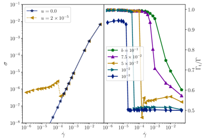
Figure 6: (Left) Flow curves of repulsive ($u=0.0$) and attractive ($u=2\times 10^{-5}$) systems in the under-damped regime ($b=5\times 10^{-2}$). The volume fraction is $\phi=0.75$. The repulsive curve exhibits the well-known Bagnold scaling, $\sigma\propto\dot{\gamma}^{2}$. (Right) The ratio of the tangential to total dissipation power in the under-damped regime. The attraction range and the volume fraction are $u=2\times 10^{-5}$ and $\phi=0.75$.

The crucial information is obtained when one splits the dissipated energy rate $\Gamma$ (which determines the stress via $\Gamma=\sigma\dot{\gamma}L^{2}$) into “tangential” and “normal” contributions $\Gamma=\Gamma_{t}+\Gamma_{n}$. As energy is only dissipated in particle contacts, one can write

$$\Gamma=\sum_{i=0}^{N}\vec{F}_{i,\text{diss.}}\cdot\vec{v}_{i}.$$ (8)

In Eq. (8), $\vec{F}_{i,\text{diss.}}$ and $\vec{v}_{i}$ determine the damping force (Eq. (2)) exerted on and the velocity of the $i$th particle. Splitting the particle velocities into components normal and tangential with respect to the contact line of the two contacting particles one obtains the associated contributions to the dissipated power.

Fig. 6 (right panel) displays the ratio of tangential to total dissipation power $\Gamma_{t}/\Gamma$. The discontinuity in the flow curve is visible as a discontinuous drop of the fraction of dissipation in the tangential channel. At small strainrates, as anticipated above, dissipation is completely dominated by the tangential motion of particles around each other. In the Bagnold branch at high strainrates, on the other hand, dissipation is equally distributed in both channels, indicative of random particle encounters in two-particle collisions.

Thus, we can conclude, that the origin of the discontinuity is two-fold: first attractive particle interaction condense the particles into a highly coordinated (yield-stress) fluid state, that involves an overwhelming tangential contribution to energy dissipation. This fluid comes to rest at the yield stress. When, by increasing strainrates, particle momenta become too large, the cohesive force is marginalized and the network is destroyed resulting in a gas-like state with two-particle collisions and equi-partition between normal and tangential energy dissipation.

These findings allow for a comparison with the phenomenon of friction-induced shear thickening Heussinger (2013). In that scenario it is the solid-solid friction between particles that allows for a tangential channel of energy dissipation. This incurs the coexistence of two branches in the flowcurves, a yield-stress branch and a flowing state, that can either be viscous or Bagnold in nature. When the stress reaches a certain threshold the flowing state becomes metastable, followed by a discontinuous transition into the yield-stress branch, which has a much higher stress. This gives rise to the phenomenon of discontinuous shear thickening.

Here, the presence of a tangential dissipation channel also gives rise to the two states with high and low $\Gamma_{t}$, respectively. Interestingly, however the stabilities of the two branches are reversed as compared to the frictional scenario: the yield stress branch is stable at small strainrates, while the Bagnold fluid is stable at high strainrates. Thus, in general the stress decreases discontinuously, and one can speak of discontinuous shear thinning. One has to be careful, however. There is one instance in Fig. 2, where the stress does not decrease but increase. This happens at the smallest available damping $b=10^{-3}$. The reason for this inversion is the opposite dependence on $b$ of the two branches. While the yield stress branch decreases, the Bagnold branch increases upon decreasing $b$.

Pursuing the analogy with the frictional scenario further, we test for the dependence on volume fraction $\phi$. In Fig. 7, we show the flow curve as well as the corresponding viscosity, for one such set of $u$ and $b$, with changing $\phi$. The discontinuous shear thinning, from the yield stress branch to the inertial branch, evolves out of a continuous shear thinning, quite similar to the frictional scenario. Again, the trend is reversed, however. With friction, it is the increase of volume fraction that triggers the transition from continuous to discontinuous shear thickening Maiti et al. (2016). Here, it is the decrease of volume fraction. This follows from the reversed stability in terms of strainrate and the fact that the yield-stress branch is more stable at higher volume-fraction.

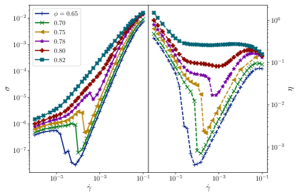
Figure 7: (Left) Flow curves, i.e. stress $\sigma$ vs. strainrate $\dot{\gamma}$, at $u=2\times 10^{-5}$, $b=5\times 10^{-2}$ and different $\phi$. (Right) Corresponding data for viscosity, $\eta({\dot{\gamma}})$.

In the frictional system, because of the properties of the frictional interaction, it is only at high pressures that particles can condense into network-like structures. Then it is possible that the frictional dissipation is enhanced beyond what one would expect from simple two-particle collisions in a granular gas. Pressure increases both with volume-fraction and strainrate. On the other hand, adhesion strength is independent of strainrate and faster motion thus weakens the network and triggers a transition into the fluid.

III.0.4 Shear bands

With the phenomenon of discontinuous shear thinning we open up the possibility for flow instabilities.

In the frictional scenario of discontinuous shear-thickening unsteady chaotic flow Grob et al. (2016); Hermes et al. (2016) and vorticity banding has been observed Chacko et al. (2018). On the other hand, a decreasing flowcurve is prone to the formation of shear bands in the gradient directionLong simulations in large enough systems are necessary to make these instabilities observable. Indeed, we can identify shear bands in the vicinity of the discontinuity when we perform ramping simulations. In these simulation we slowly ramp up the strainrate after a strain of $\gamma_{\rm tot}=40$, until we reach high enough strainrates and the ramp is reversed. The associated flowcurve encircling the discontinuity is depicted in Fig. 8.

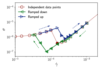
Figure 8: Flowcurve for a strainrate ramp. Hysteresis and shear bands for a system with $u=2\times 10^{-5}$, $\phi=0.75$ and $b=5\times 10^{-2}$. Filled symbols indicate where shear bands are observed.

Next to an extended hysteresis loop we find evidence of shear banded states. These are highlighted by filled symbols in the figure. Interestingly, the average stress in these shear-banded states does not differ much from the value in the homogeneous state (it is somewhat larger). Also, there is no indication of a stress plateau. Such a plateau would be indicative of a scenario where the two coexisting bands represent states (at equal stress) from an underlying non-banded local flowcurve Dhont (1999).

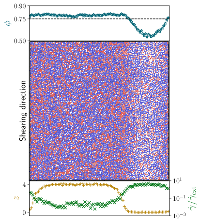
Figure 9: Snapshot of a shear-banded system with $N=10^{4}$, $b=5\times 10^{-2}$, $u=2\times 10^{-5}$, $\phi=0.75$ and imposed strainrate $\dot{\gamma}_{\rm ext}=2\times 10^{-4}$. Panels at top and bottom highlight the local values of volume fraction $\phi$ as well as connectivity $z$ and strainrate $\dot{\gamma}/\dot{\gamma}_{\rm ext}$. These are obtained by performing averages along slices in shearing direction.

A snapshot of a shear-banded state makes clear what is happening (Fig. 9). Next to the strainrate, the volume fraction as well as the connectivity vary between the bands. Volume fraction and connectivity are substantially reduced in the inertial band, indicating a dilute granular gas state. In the remaining system the connectivity is close to the threshold value of $z_{\rm iso}=4$, which would indicate the possibility of a solid state. It might therefore represent a quasi-solid band at a slightly elevated volume-fraction $\phi>0.75$. Interestingly, the interface between the two bands seems to have an even higher density, even though the connectivity is markedly reduced and interpolates from the high value of the solid to the small value of the gas. Such an anti-correlation between connectivity and density is also observable in our previous work Irani et al. (2014, 2016), where the tangential channel of energy dissipation is absent. In that system, however, the gas-like band is absent and the solid band coexists with what here might be just an interface. We also note that such changes in local density, during shearband formation, has also been observed in experiments involving discontinuous shear-thickening Fall et al. (2015).

Larger systems are necessary to study these questions in more detail. It might also be interesting to add a third spatial dimension to study the possibility of vorticity banding in the presence of discontinuities in the flowcurves Chacko et al. (2018).

IV Conclusion

The system is quite similar to the one studied by Nicolas et al. Nicolas et al. (2016) with two important differences. The first relates to the presence, in the current work, of a tangential channel of energy dissipation. The second to the type of adhesion forces. Nicolas et al. use a standard Lennard-Jones interaction, where the range of attraction is on the order of the diameter of the repulsive core. In our system repulsive core (particle diameter $d=1$) and attraction range $ud$ are scale separated and $u\ll 1$. Thus, attractive forces are really only active when particles are near contact.

The resulting solid is therefore very fragile in the sense that the number of interactions (“contacts”) is just slightly above the minimum isostatic value, $\delta\!z=z-z_{\rm iso}\ll 1$. This allows us on the one hand to derive a scaling expression for the yield stress $\sigma_{y}\sim u^{1/2}\delta\!z^{3/2}$. On the other hand, the yield stress is very small and not accessible in our work. Instead we observe an extended Herschel-Bulkley (HB) regime $\sigma\sim\dot{\gamma}^{\nu}$ with an exponent $\nu\approx 0.45$ quite similar to other studies (Nicolas et al. have $\nu=0.5$). We tried to also relate this exponent to the underlying isostatic structure but so far without success.

In underdamped systems a weakening effect sets in and the stress is reduced below the HB branch. This is due to an effective temperature that originates in enhanced velocity fluctuations in weakly damped systems. The resulting $T^{2/3}$ scaling of the stress follows the theory proposed in Refs. Johnson and Samwer (2005); Chattoraj et al. (2010). The same scaling is observed in Nicolas et al. however, the scaling of the shear-induced temperature $T$ itself is different in that work. There, the energy balance argument Eq. (5) is used to derive (the equivalent of our notation)

$$T\sim m\dot{\gamma}^{2}\text{Wi}^{-1}$$ (9)

which is valid as long as the stress scale is set just by attractive forces $\sigma\sim\epsilon u$. Here, however, it is far away from the yield point deep in the flowing region, where the weakening effect sets in. The relevant stress scale therefore is the HB result, $\sigma\sim\epsilon u\text{Wi}^{\nu}$ and $T\sim m\dot{\gamma}^{2}\text{Wi}^{\nu-1}$. This is also why for weak inertial effects the stress does not decrease as a function of strainrate, as in Ref.Nicolas et al. (2016). Rather, the stress reduction $\Delta\sigma_{\rm th}$ superimposes on the HB law $\sigma\sim\epsilon u\text{Wi}^{\nu}$, which in effect leads to a weaker increase or to an intermediate plateau in stress (see Fig. 2). Only for the weakest damping do we actually observe a negative slope in the flowcurve.

Finally, no shear bands are observed in Nicolas et al.. Here, we do observe a shear banding instability, albeit the scenario is quite complex and associated with a discontinuity in the flowcurve which does not directly follow from the weakening effect just described.

Rather, we set up an analogy with frictional systems, where the phenomenon of discontinuous shear-thickening can be interpreted as a coexistence (spatial or temporal) of two disconnected branches of the flowcurve. Due to the nature of the frictional interaction, the fluid branch is stable at low volume-fractions and small strainrates. Increasing the strainrates the system jumps to the HB branch, which is at higher stress. In the adhesive system discussed here, the same two branches are present but the roles and stabilies are reversed. At small densities and strainrates the solid HB branch is stable – the particles condense into a network- or gel-like inhomogeneous structure. Increasing the strainrate the structure of the network is weakened and the system jumps into the fluid branch, which is at lower stress. Thus the system undergoes discontinuos shear thinning. The crucial ingredient to observe these discontinuities in both cases is a tangential channel of energy dissipation, i.e. due to velocities directed tangentially to the particle surface. It will be interesting to see if these effects can be generalized to other dissipation models, for example lubrication forces, which also have normal and tangential modes. Future work should also study Brownian systems to address the interplay between real and shear-induced temperature.