PDE-based numerical method for a limited angle X-ray tomography

Abstract

A new numerical method for X-ray tomography for a specific case of incomplete Radon data is proposed. Potential applications are in checking out bulky luggage in airports. This method is based on the analysis of the transport PDE governing the X-ray tomography rather than on the conventional integral formulation. The quasi-reversibility method is applied. Convergence analysis is performed using a new Carleman estimate. Numerical results are presented and compared with the inversion of the Radon transform using the well-known filtered back projection algorithm. In addition, it is shown how to use our method to study the inversion of the attenuated X-ray transform for the same case of incomplete data.

35R30, 44A12

1 Introduction

Computing a function from its Radon transform, which was first introduced by Radon in 1917 [35, 36], is considered as the theory behind the first commercial computed tomography (CT) scanner, invented by Hounsfield. Due to this contribution, Hounsfield was awarded the Nobel prize in 1979. In the current paper, we develop a new numerical method for this inverse problem for the case of a special type of limited angle data for the Radon transform. This type of limited angle data might find applications in checking out baggages in airports as well as checking out interior structures of walls.

The Radon transform of a function $f$ is the integral of $f$ on a set of segments of straight lines. If that set includes all straight lines in the plane, we say that the Radon transform transform data are completely given. The exact reconstruction of the function $f$ from its complete Radon transform data can be computed by the well-known filtered back projection algorithm, see [29, 34]. The full observation of the data is important since the filtered back projection formula involves a non local operator. In some applications, due to some technical reasons, the complete Radon transform cannot be collected. We refer the reader to [5, 6, 7] for some circumstances about this incompleteness, e.g., when the $X$-rays are blocked by metal bars, see [5, Section 7] for a detailed discussion. On the other hand, in this paper, we design another experimental situation in which a large amount of the Radon data is lost, see Section 2. Our goal is to image objects (or equivalently to determine a function) when an interval of view angles is limited in a special way. This situation includes Radon transform for the limited angle problem [27]. The missing data leads to the instability of the reconstruction. We cite some important papers [1, 5, 13, 30, 31] and references therein that characterize and (or) introduce the strategies to reduce the resulting artifacts, which appear in the reconstructed image. To treat the case of incompleteness, one might non-rigorously fill the missing data by the number $0$, see figures 2-4 in [5].

In this paper, we propose a new numerical method which analytically and numerically produces a good approximation of the inversion of the Radon transform for a special case of limited angle data. Unlike the filtered back projection algorithm, our approach is not based on the integral form of the Radon transform and is not intended to derive an explicit inversion formula. We use a boundary value problem for a linear partial differential system whose solution directly yields the solution to the inverse problem. Instead of using the conventional “integral” approach, we consider a well known PDE [14] governing the propagation of X-rays. In fact, this is the stationary transport PDE without absorption and integral terms. That PDE involves two unknown functions: its solution $u$ and the target function of interest $f$. At each point of the boundary, one of boundary conditions for $u$ is exactly the integral along a line segment, which is considered in Radon transform. In fact, boundary conditions for that PDE are over determined ones. Using one of ideas of the Bukhgeim-Klibanov method [10], we next differentiate that PDE with respect to the source location to obtain another PDE, in which the function $f$ is not involved, see [20] for a survey of the method of [10] as well as books [3, 4, 19]. That new equation contains the unknown function $u$ as well as its partial derivative with respect to the source location. However, a theory on how to solve the resulting over determined boundary value problem is not available yet. In this paper, we only approximate the solution of this problem by the solution of an overdetermined boundary value problem for a linear system of coupled PDEs of the first order. The solution of the latter problem is used to compute a partial sum of the Fourier series for the function $u$ with respect to a special orthonormal basis. This “cut-off” technique was first introduced in [23] for a class of coefficient inverse problems. Then, it was successfully applied to numerically solve some coefficient inverse problems [24, 25]. Having that approximation for the function $u$ in hands, we compute the corresponding approximation for the function $f$ directly.

As mentioned in the above paragraph, to obtain that system of PDEs, we truncate the Fourier series with respect to a special orthonormal basis and assume that the corresponding approximation of the function $u$ still satisfies the above mentioned PDE. Let $N$ be the number of terms of that truncated series. Even though the original series converges of course as $N\rightarrow\infty,$ the question about the convergence of resulting numerical solutions as $N\rightarrow\infty$ is a very challenging one. The true “hidden” reason of this challenge is the ill-posedness of the originating problem. Thus, we do not provide here the proof of convergence of those numerical solutions at $N\rightarrow\infty$. We estimate an optimal number $N$ numerically, see Remark 5.3 in Section 5.4. In other words, we consider an approximate mathematical model, which is a common place in numerical methods for ill-posed problems. Indeed, it is well known that proofs of convergence of numerical solutions resulting from truncations of a variety of Fourier series, as $N\rightarrow\infty,$ are quite challenging ones in many other inverse/ill-posed problems. Hence, these proofs are usually omitted. Still, it is also well known that approximate mathematical models based on truncated Fourier series work successfully numerically even for coefficient inverse problems, which are nonlinear, unlike the linear problem of this paper. As some examples of those successes, we refer to, e.g. works of Kabanikhin with coauthors [15, 16, 17] for the 2D version of the Gelfand-Levitan-Krein method, as well as to publications [22, 24, 25] of the first author with coauthors.

The above mentioned overdetermined boundary value problem for a system of PDEs of the first order is solved here by the quasi-reversibility method, which is well known to be a perfect tool to solve overdetermined boundary value problems for PDEs. This method was first introduced by Lattès and Lions [28] for numerical solutions of ill-posed problems for PDEs. It has been studied intensively since then, see e.g., [2, 8, 9, 11, 12, 18, 20, 32]. A recent survey on this method can be found in [21].

In the convergence analysis of this paper we consider a semi discrete form of our system of PDEs, which is more realistic for computations than the conventional continuous form. More precisely, we assume that partial derivatives with respect to one of two variables are written in finite differences, whereas derivatives with respect to the second variable are written in the conventional continuous form. However, we do not allow the step size of the grid $h\rightarrow 0,$ unlike many conventional well posed problems for PDEs. Indeed, the analysis at $h\rightarrow 0$ is a very challenging one due to the ill-posedness of the problem. As to the fully discrete form, in which both partial derivatives are written via finite differences, it is clear from, e.g. [18], that, in the case of ill-posed problems (as opposed to some conventional well posed problems for PDEs), this case is far more complicated. Thus, it is not considered in this first publication about our new method.

It is well known that proofs of convergence of regularized solutions of the quasi-reversibility method are based on Carleman estimates, see, e.g. [20, 21]. Hence, first, we prove a new Carleman estimate. Next, using this estimate, we prove the existence and uniqueness of the minimizer (i.e., the regularized solution [37]) for our semi discrete version of the quasi reversibility method. Finally, using the same Carleman estimate, we establish a convergence rate of regularized solutions to the exact solution.

An important part of the paper is devoted to the numerical implementation of our method. We present here some numerical results. In particular, we compare performance of our method with the performance of the filtered back projection algorithm in which the missed data are filled by zeros. We point out that, at this early stage of the development, we are not interested in treating fine details, such as artifacts, for example. Rather, we arrange a simple post processing.

The paper is organized as follows. In Section 2 we state the problem. In Section 3 we derive the above mentioned overdetermined boundary value problem for a system of PDEs of the first order, which does not contain the target function $f$. In Section 4 we introduce first the quasi-reversibility method to solve that problem.  Next, we prove a new Carleman estimate and use this Carleman estimate to prove the existence and uniqueness of the minimizer and establish the convergence rate of the minimizers to the exact solution as the level of the measurement noise tends to zero. In Section 5 we discuss the numerical implementation of our method. Numerical studies are described in Section 6. We present concluding remarks in Section 7. In addition, we explain in Section 7 how to extend our approach to solve the inverse attenuated tomographic problem. Below all functions are real valued ones.

2 Problem statement

Everywhere below all functions are real valued ones and $\mathbf{x}=\left(x,y\right)$ denotes points in $\mathbb{R}^{2}.$ Let $b>a>0$ and $d,R>0$ be some numbers. Consider the rectangle $\Omega\subset\mathbb{R}^{2}$

(2.1) $$\Omega=(-R,R)\times(a,b).$$

Let $\Gamma_{d}\subset\mathbb{R}^{2}$ be the segment of the horizontal line where our point sources are located,

(2.2) $$\Gamma_{d}=\left\{\mathbf{x}=\left(x,y\right):x\in(-d,d),y=0\right\}.$$

Let $f(\mathbf{x})$ be the unknown function whose support is contained in $\Omega$, i.e.

(2.3) $$f\left(\mathbf{x}\right)=0\text{ for }\mathbf{x}\in\mathbb{R}^{2}\setminus\Omega.$$

For the purpose of our theoretical analysis, we assume below that $f\in C^{2}(\mathbb{R}^{2}).$ In the case of X-ray tomography the function $f\left(\mathbf{x}\right)$ represents the X-ray attenuation coefficient at the point $\mathbf{x}$, see [29]. Consider point sources $\mathbf{x}_{\alpha}=\left(\alpha,0\right)\in\Gamma_{d}.$ We define the function $u(\mathbf{x},\mathbf{x}_{\alpha})$ as

(2.4) $$u(\mathbf{x},\mathbf{x}_{\alpha})=\int_{L(\mathbf{x},\mathbf{x}_{\alpha})}f(\mathbf{\xi})d\sigma,\quad$$

where $L(\mathbf{x},\mathbf{x}_{\alpha})$ is the line segment connecting points $\mathbf{x}$ and $\mathbf{x}_{\alpha}$. We are interested in the following problem:

Problem 2.1 (Tomographic inverse problem with incomplete data).

Determine the function $f$ from the measurement of $Rf$, where

(2.5) $$Rf=u(\mathbf{x},\mathbf{x}_{\alpha})$$

for all $\mathbf{x}=(x,y)\in\partial\Omega$ and all $\mathbf{x}_{\alpha}=(\alpha,0)\in\Gamma_{d}.$ The function $Rf$ is known as the Radon transform of the function $f$.

Remark 2.1.

The Radon transform, along with the inversion formula, was first introduced by Radon in 1917 in his celebrated paper [35]. We also refer the reader to [36] for the translation of [35] into English .

The case when the data $Rf(\mathbf{x},\mathbf{x}_{\alpha})$ are available for all $\mathbf{x}_{\alpha}$ and $\mathbf{x}$ such that the set of lines $L(\mathbf{x},\mathbf{x}_{\alpha})$ contains all possible lines intersecting $\Omega$, Problem 2.1 is known as the tomographic inverse problem with complete data. This inverse problem with complete data is exactly solved by the filtered back projection formula [29]. Unlike this, in the current paper, the point source $\mathbf{x}_{\alpha}$ is allowed to “move” only along the line segment $\Gamma_{d}$, which is located below $\Omega,$ rather than on a curve surrounding $\Omega,$ as illustrated in Figure 1. In this setting, one can easily find many straight lines intersecting $\Omega$ but not belonging to our set of lines $L(\mathbf{x},\mathbf{x}_{\alpha}).$ Therefore, the data in Problem 2.1 is said to be incomplete. See Figures 2b–5b versus Figures 2c–5c for the illustrations of the amount of missing data.

Due to a large amount of missing data, the Radon inversion via the well-known filtered back projection algorithm built in MATLAB does not work well. In addition, this formula is not rigorously established for this case. These motivate us to develop a new numerical method to solve Problem 2.1. We use the well-known transport PDE that governs the function $Rf$. Next, we establish and solve an inverse source problem for this equation. This is our PDE approach.

Problem 2.1 arises in X-ray tomography. Assume that we want to image an object in a 3D domain $Q$, illustrated on Figure 1a. A source, located at each point $\mathbf{x}_{\alpha}$ on the line $\Gamma_{d}$ in (2.2) below $Q$, generates tomographic data that can be measured at an array of detectors on a rectangle on the top of $Q$. One can arrange such detectors on a set of “observation lines” that are parallel to $\Gamma_{d}$. Each observation line, together with $\Gamma_{d}$, defines a plane. The cross section of $Q$ by that plane is our 2D domain $\Omega$. Figure 1b illustrates an example of such cross section. Hence, we believe that results of this paper have potential applications in, e.g. checking out a bulky baggage in airports.

We next discuss the issue of the data for Problem 2.1 on the boundary of $\Omega$. The data on the top of $\Omega$ can be collected directly. As to the data on two vertical sides of $\Omega,$ one can easily see from Figure 1b that if the measurement line is sufficiently long, then we can calculate the data on the sides of $\Omega$ using the data on the measurement side as well as (2.3) and (2.4). Also, by (2.3) and (2.4) the data on the bottom side of $\Omega$ is identically zero. Solving problem 2.1 provides a knowledge of a cross section of the desired object.

(a) A diagram for the experiment set up.

(b) A cross section $\Omega$ of $Q$

Figure 1: An illustration of a 3D tomographic experiment. One can detect the 3D object in $Q$ by repeatedly solving Problem 2.1 at each cross section $\Omega$ of $Q$ on the plane defined by the line of source and each observation line. In (b), $\mathbf{x}$ represents the location of detectors and $\mathbf{x}_{\alpha}$ denotes the locations of the source. In this tomographic setting, the line $L(\mathbf{x},\mathbf{x}_{\alpha})$ in (b) is assumed to be the geodesic line connecting $\mathbf{x}_{\alpha}$ and $\mathbf{x}$.

Remark 2.2 (A non uniqueness example and the uniqueness of Problem 2.1).

It is not hard to verify that $f(x,y)=h(y)$, for some function $h(y)$ satisfying

$$\int_{a}^{b}h(y)dy=0,$$

is in the null space of the “incomplete” Radon transform whose domain is all pairs $(\mathbf{x},\mathbf{x}_{\alpha})$ where $\mathbf{x}$ is on the top of $\Omega$ and the line $L(\mathbf{x},\mathbf{x}_{\alpha})$ does not intersect the vertical sides of $\Omega$. Hence, the knowledge of data for Problem 2.1 on the vertical sides of $\Omega$ is crucial. The uniqueness of Problem 2.1 is considered as an assumption in this paper. On the other hand, we consider in this paper an approximate mathematical model, which is obtained via the truncation of a certain Fourier series. Uniqueness for the latter case follows immediately from our convergence result (Theorem 4.7).

Lemma 2.1.

Assume that the function $f\in C^{k}(\mathbb{R}^{2})$, $k\geq 1$ and satisfies condition (2.3). Then, the function $u(\mathbf{x},\mathbf{x}_{\alpha})=Rf(\mathbf{x},\mathbf{x}_{\alpha})$ is $k$ times continuously differentiable with respect to both $\mathbf{x}\in\Omega$ and $\alpha\in(-d,d)$. Moreover, those derivatives are bounded in $\overline{\Omega}\times[-d,d].$

Proof. We have

$$L(\mathbf{x},\mathbf{x}_{\alpha}) =\left\{\mathbf{x}\left(t\right)=\left(1-t\right)\mathbf{x}_{\alpha}+t\mathbf{x,}\quad t\in\left(0,1\right)\right\}$$

$$=\left\{\left(x(t),y(t)\right):x\left(t\right)=\alpha+t\left(x-\alpha\right),y\left(t\right)=ty,\quad t\in\left(0,1\right)\right\}.$$

Hence, by (2.4)

$$u(\mathbf{x},\mathbf{x}_{\alpha})=\int_{L(\mathbf{x},\mathbf{x}_{\alpha})}f(\mathbf{\xi})d\sigma=\sqrt{\left(x-\alpha\right)^{2}+y^{2}}\int_{0}^{1}f\left(\alpha+t\left(x-\alpha\right),ty\right)dt.\text{ }\square$$

3 An approximation for the model governing the X-ray tomographic data

We establish in this section a system of first order PDEs that leads to our numerical method to solve Problem 2.1.

3.1 The exact PDE governing the X-ray tomographic function

For each source $\mathbf{x}_{\alpha}=(\alpha,0)$ in $\Gamma_{d}$ and $\mathbf{x}=(x,y)$ in $\Omega$, let $\varphi$ be the angle constituted by the line $L(\mathbf{x},\mathbf{x}_{\alpha})$ and the $x-$axis. The directional derivative of $u(\mathbf{x},\mathbf{x}_{\alpha})$ with respect to the direction $(\cos\varphi,\sin\varphi)$ of the line $L(\mathbf{x},\mathbf{x}_{0})$ is given by

$$\cos\varphi u_{x}+\sin\varphi u_{y} =\lim_{t\rightarrow 0}\frac{u(x+t\cos\varphi,y+t\sin(\varphi),\mathbf{x}_{\alpha})-u(x,y,\mathbf{x}_{\alpha})}{t}$$

$$=\lim_{t\rightarrow 0}\frac{1}{t}\int_{l_{t}}f(\sigma)d\sigma$$

where $l_{t}\subset L(\mathbf{x},\mathbf{x}_{0})$ is the line connecting the point $\mathbf{x}$ and $(\mathbf{x}+t(\cos\varphi,\sin\varphi))$. Since the length of $l_{t}$ is $t$ and the function $f$ is continuous, then the above limit is $f(\mathbf{x})$. Since

$$\cos\varphi=\frac{x-\alpha}{|\mathbf{x}-\mathbf{x}_{\alpha}|}=\frac{x-\alpha}{\sqrt{\left(x-\alpha\right)^{2}+y^{2}}}\text{ and }\sin\varphi=\frac{y}{|\mathbf{x}-\mathbf{x}_{\alpha}|}=\frac{y}{\sqrt{\left(x-\alpha\right)^{2}+y^{2}}},$$

for each $\mathbf{x}_{\alpha}=(\alpha,0)$, $\alpha\in(-d,d)$, then the function $u(\mathbf{x},\mathbf{x}_{\alpha})$ satisfies the following form of the transport equation:

(3.1) $$\frac{x-\alpha}{|\mathbf{x}-\mathbf{x}_{\alpha}|}u_{x}+\frac{y}{|\mathbf{x}-\mathbf{x}_{\alpha}|}u_{y}=f(x,y).$$

Remark 3.1.

Although equation (3.1) is well known, see e.g., [14], we have briefly derived it as above. This is because equation (3.1) leads us to a PDE approach to solve the tomographic inverse problem with incomplete data, Problem 2.1. Equation (3.1) is the exact mathematical model that governs the function $u$.

3.2 An orthonormal basis in $L^{2}(-d,d)$

We start by recalling a special orthonormal basis of $L^{2}(-d,d)$ that is different from the basis constructed from either standard orthonormal polynomials or trigonometric functions. If one considers such a usual basis of $L^{2}(-d,d)$, then one of the elements of that basis is a constant, meaning that its derivative is identically zero. Unlike this, for our approach, we need to construct an orthonormal basis $\left\{\Psi_{n}\left(\alpha\right)\right\}_{n=1}^{\infty}$ in $L_{2}(-d,d),$ which has the following two properties:

1. $\Psi_{n}\in C^{1}\left[-d,d\right],$ $\forall n=1,2,\dots$

2. Let $\left(,\right)$ denotes the scalar product in $L^{2}\left(-d,d\right)$ and let $a_{mn}=\left(\Psi_{n}^{\prime},\Psi_{m}\right).$ Then the matrix $M_{N}=\left(a_{mn}\right)_{m,n=1}^{N}$ should be invertible for any $N=1,2,\dots$

Such a basis was first constructed in [23]. We now reproduce that construction for the convenience of the reader. For $\alpha\in(-d,d)$, consider the set of functions $\{\alpha^{n-1}e^{\alpha}\}_{n=1}^{\infty}$. These functions are linearly independent and form a complete set in $L^{2}(-d,d)$. Applying the classical Gram-Schmidt orthonormalization procedure to this set, we obtain the orthonormal basis $\{\Psi_{n}\left(\alpha\right)\}_{n=1}^{\infty}$ of $L^{2}(-d,d)$. It is obvious that for each $n\geq 1$, $\Psi_{n}(\alpha)=P_{n-1}(\alpha)e^{\alpha}$, where $P_{n-1}$ is a polynomial of the degree $n-1$. The following lemma holds true:

Lemma 3.2 (Theorem 2.1 in [23]).

The function $\Psi_{n}^{\prime}$ is not identically zero for any $n\geq 1$. Moreover, we have

$$\phi_{mn}=\int_{-d}^{d}\Psi_{n}^{\prime}(\alpha)\Psi_{m}(\alpha)d\alpha=\left\{\begin{array}[]{ll}1&\mbox{if }n=m,\\ 0&\mbox{if }n<m.\end{array}\right.$$

Consequently, for any integer $N\geq 1$, the matrix $M_{N}=(\phi_{mn})_{m,n=1}^{N}$ has determinant 1 and is, therefore, invertible.

The function $u(x,y,\alpha)$ can be represented via the following Fourier series, which converges in $L^{2}(-d,d)$ for every point $\left(x,y\right)\in\overline{\Omega}:$

$$u(x,y,\alpha)=\sum_{n=1}^{\infty}u_{n}(x,y)\Psi_{n}(\alpha),\quad(x,y)\in\overline{\Omega},\alpha\in(-d,d).$$

In order to introduce our approximate mathematical model mentioned in Introduction, we approximate the function $u(\mathbf{x},\mathbf{x}_{\alpha})=u(x,y,\alpha)$ as:

(3.2) $$u(x,y,\alpha)\approx\sum_{n=1}^{N}u_{n}(x,y)\Psi_{n}(\alpha),\quad(x,y)\in\overline{\Omega},\alpha\in(-d,d),$$

where $N\geq 1$ is a certain integer, which is chosen later numerically, and

(3.3) $$u_{n}(x,y)=\int_{-d}^{d}u(x,y,\alpha)\Psi_{n}(\alpha)d\alpha,\quad(x,y)\in\overline{\Omega},\alpha\in(-d,d).$$

Our approximate mathematical model mentioned in the Introduction amounts to the replacement in (3.2) “$\approx$” with “$=$” as well as to the assumption that the resulting function solves equation (3.1). Thus, everywhere below

(3.4) $$u(x,y,\alpha)=\sum_{n=1}^{N}u_{n}(x,y)\Psi_{n}(\alpha),\text{ \ }(x,y)\in\overline{\Omega},\alpha\in(-d,d).$$

3.3 A system of first order PDEs

The goal of this section is to derive a system of linear coupled PDEs, whose solution directly yields numerical solution to Problem 2.1. Differentiating equation (3.1) with respect to $\alpha$ and denoting $v=\partial_{\alpha}u$, we obtain

(3.5) $$\frac{x-\alpha}{\left|\mathbf{x}-\mathbf{x}_{\alpha}\right|}v_{x}+\frac{y}{\left|\mathbf{x}-\mathbf{x}_{\alpha}\right|}v_{y}-\frac{y^{2}}{\left|\mathbf{x}-\mathbf{x}_{\alpha}\right|^{3}}u_{x}+\frac{(x-\alpha)y}{\left|\mathbf{x}-\mathbf{x}_{\alpha}\right|^{3}}u_{y}=0$$

for all ${\bf x}=(x,y)\in\Omega$ and $\alpha\in(-d,d).$ Equation (3.5) is equivalent with

(3.6) $$v_{y}=-\frac{x-\alpha}{\left|\mathbf{x}-\mathbf{x}_{\alpha}\right|^{2}}u_{y}-\frac{x-\alpha}{y}v_{x}+\frac{y}{\left|\mathbf{x}-\mathbf{x}_{\alpha}\right|^{2}}u_{x},\text{ \ }\mathbf{x}=(x,y)\in\Omega,\alpha\in(-d,d).$$

By (3.4) the function $v(x,y,\alpha)$ can be written as

(3.7) $$v(\mathbf{x},\alpha)=\sum_{n=1}^{N}u_{n}(\mathbf{x})\Psi_{n}^{\prime}(\alpha),\quad\mathbf{x}=(x,y)\in\overline{\Omega},\alpha\in(-d,d).$$

Plugging the function $u$ and $v$ in (3.4) and (3.7) respectively into (3.6), we obtain

(3.8) $$\sum_{n=1}^{N}\partial_{y}u_{n}(\mathbf{x})\Psi_{n}^{\prime}(\alpha)=-\frac{x-\alpha}{\left|\mathbf{x}-\mathbf{x}_{\alpha}\right|^{2}}\sum_{n=1}^{N}\partial_{y}u_{n}(\mathbf{x})\Psi_{n}(\alpha)\\ -\frac{x-\alpha}{y}\sum_{n=1}^{N}\partial_{x}u_{n}(\mathbf{x})\Psi_{n}^{\prime}(\alpha)+\frac{y}{\left|\mathbf{x}-\mathbf{x}_{\alpha}\right|^{2}}\sum_{n=1}^{N}\partial_{x}u_{n}(\mathbf{x})\Psi_{n}(\alpha)$$

for all ${\bf x}=(x,y)\in\Omega$ and $\alpha\in(-d,d).$ Multiplying both sides of (3.8) by $\Psi_{m}(\alpha)$, $m\in\{1,\dots,N\}$, and then integrating the resulting equation with respect to $\alpha\in(-d,d)$, we obtain

$$\sum_{n=1}^{N}\partial_{y}u_{n}(\mathbf{x})\int_{-d}^{d}\Psi_{m}(\alpha)\Psi_{n}^{\prime}(\alpha)d\alpha=-\sum_{n=1}^{N}\partial_{y}u_{n}(\mathbf{x})\int_{-d}^{d}\frac{x-\alpha}{\left|\mathbf{x}-\mathbf{x}_{\alpha}\right|^{2}}\Psi_{m}(\alpha)\Psi_{n}(\alpha)d\alpha\\ +\sum_{n=1}^{N}\partial_{x}u_{n}(\mathbf{x})\int_{-d}^{d}\left(-\frac{x-\alpha}{y}\Psi_{m}(\alpha)\Psi_{n}^{\prime}(\alpha)+\frac{y}{\left|\mathbf{x}-\mathbf{x}_{\alpha}\right|^{2}}\Psi_{m}(\alpha)\Psi_{n}(\alpha)\right)d\alpha.$$

Recalling Lemma 3.2, we obtain

(3.9) $$M_{N}\mathbf{U}_{y}(\mathbf{x})=D_{1}\left(\mathbf{x}\right)\mathbf{U}_{y}(\mathbf{x})+D_{2}\left(\mathbf{x}\right)\mathbf{U}_{x}(\mathbf{x}),\quad\mathbf{x}=(x,y)\in\Omega,$$

where the $N-$ dimensional vector valued function $\mathbf{U}\left(\mathbf{x}\right)$ is

(3.10) $$\mathbf{U}\left(\mathbf{x}\right)=\left(u_{1},\dots,u_{N}\right)^{T}\left(\mathbf{x}\right)$$

and $D_{1}\left(\mathbf{x}\right),D_{2}\left(\mathbf{x}\right)$ are two $N\times N$ matrices whose $mn^{\mathrm{th}}$, $1\leq m,n\leq N$, entries

(3.11) $$(D_{1})_{mn} =\int_{-d}^{d}\frac{x-\alpha}{\left|\mathbf{x}-\mathbf{x}_{\alpha}\right|^{2}}\Psi_{m}(\alpha)\Psi_{n}(\alpha)d\alpha,$$

(3.12) $$(D_{2})_{mn} =\int_{-d}^{d}\left(-\frac{x-\alpha}{y}\Psi_{m}(\alpha)\Psi_{n}^{\prime}(\alpha)+\frac{y}{\left|\mathbf{x}-\mathbf{x}_{\alpha}\right|^{2}}\Psi_{m}(\alpha)\Psi_{n}(\alpha)\right)d\alpha$$

belong to $C^{\infty}\left(\overline{\Omega}\right).$ The following lemma follows immediately from (3.11) and (3.12):

Lemma 3.3.

Suppose that in the definition (2.1) of the domain $\Omega$ the number $a>1.$ Then the following estimates hold:

$$\max_{\mathbf{x}\in\overline{\Omega}}\left\|D_{1}\left(\mathbf{x}\right)\right\|\leq\frac{C_{1}}{a^{2}},\text{ }\max_{\mathbf{x}\in\overline{\Omega}}\left\|D_{2}\left(\mathbf{x}\right)\right\|\leq\frac{C_{1}}{a}.$$

Remark 3.4.

The system of PDEs (3.9) for the $N$-dimensional vector valued function $\mathbf{U}(\mathbf{x})$ is our approximate mathematical model for the exact one (3.1). Our method to solve Problem 2.1 is based on a numerical solver for (3.9).

Here and everywhere below the norm of a matrix is the square root of the sum of squares of its entries. Also, in Lemma 3.15 and everywhere below $C_{1}=C_{1}\left(N,R,d\right)>0$ denotes different constants independent on the number $a$. Rewrite (3.9) as

(3.13) $$M_{N}\left(I-M_{N}^{-1}D_{1}\left(\mathbf{x}\right)\right)\mathbf{U}_{y}(\mathbf{x})+D_{2}\left(\mathbf{x}\right)\mathbf{U}_{x}(\mathbf{x})=0,\quad\mathbf{x}=(x,y)\in\Omega.$$

Lemma 3.15 follows immediately from Lemmata 3.2 and 3.3.

Lemma 3.5.

For each $N\geq 1$, there exists a sufficiently large number $a_{0}=a_{0}(N,R,d)>1$ such that for any $a\geq a_{0},$ the matrix $M_{N}\left(I-M_{N}^{-1}D_{1}\left(\mathbf{x}\right)\right)$ is invertible. Denote

$$D\left(\mathbf{x}\right)=-\left[M_{N}\left(I-M_{N}^{-1}D_{1}\left(\mathbf{x}\right)\right)\right]^{-1}D_{2}\left(\mathbf{x}\right)\quad{\bf x}\in\overline{\Omega}.$$

We have

(3.14) $$\max_{\mathbf{x}\in\overline{\Omega}}\left\|D\left(\mathbf{x}\right)\right\|\leq C_{1}.$$

Moreover, equation (3.13) is equivalent to

(3.15) $$\mathbf{U}_{y}(\mathbf{x})+D\left(\mathbf{x}\right)\mathbf{U}_{x}(\mathbf{x})=0,\text{ }\mathbf{x}=(x,y)\in\Omega.$$

In addition to (3.15), the following vector function $\mathbf{g}\left(\mathbf{x}\right)$ of boundary conditions is known

(3.16) $$\mathbf{U}(\mathbf{x})=\mathbf{g}(\mathbf{x}),\quad\mathbf{x}\in\partial\Omega$$

via using (3.3) and (3.10) for $\mathbf{x}=(x,y)\in\partial\Omega$. In particular

(3.17) $$\mathbf{g}\left(\mathbf{x}\right)=0\text{ for }\mathbf{x}=(x,a).$$

Thus, we solve below boundary value problem (3.15), (3.16). Suppose that we have obtained its approximate solution. Then the corresponding approximation for the target function $f\left(\mathbf{x}\right)$ should be obtained via the substitution of (3.4) in (3.1), see (4.39).

Remark 3.6.

As it was mentioned in Introduction, the number $N$ should be chosen numerically, also see Remark 5.4.

4 The Quasi-Reversibility Method for the first order system of PDEs (3.15)–(3.16)

The boundary value problem (3.15), (3.16) is overdetermined since the boundary data (3.16) for the system (3.15) of PDEs of the first order are given on the whole boundary $\partial\Omega$ rather than on its part. Therefore, to find an approximate solution of problem (3.15), (3.16), we use the quasi-reversibility method, which, in general, works properly for overdetermined problems.

For vector functions $\mathbf{U\in}H^{1}\left(\Omega\right)^{N},$ consider the functional $J_{\varepsilon}\left(\mathbf{U}\right)$

(4.1) $$J_{\varepsilon}\left(\mathbf{U}\right)=\int_{\Omega}\left|\mathbf{U}_{y}(\mathbf{x})+D\left(\mathbf{x}\right)\mathbf{U}_{x}(\mathbf{x})\right|^{2}d\mathbf{x}+\varepsilon\left\|\mathbf{U}\right\|_{H^{1}(\Omega)^{N}}^{2},$$

where $\varepsilon\in\left(0,1\right)$ is the regularization parameter. The quasi-reversibility method for problem (3.15)–(3.16) amounts to the following minimization problem:

Problem 4.1 (Solving (3.15)–(3.16) by the quasi-reversibility method in the continuous form).

Minimize functional (4.1) on the set of vector functions $\mathbf{U}\in H^{1}\left(\Omega\right)^{N},$ subject to boundary condition (3.16). The resulting minimizer is called the regularized solution of (3.15)–(3.16).

Conventionally, the convergence analysis of the quasi-reversibility method is performed on the basis of Carleman estimates [21]. However, since $\mathbf{U}\left(\mathbf{x}\right)$ is a vector function rather than a 1D function and also since the matrix $D\left(\mathbf{x}\right)$ is likely not self adjoint, we cannot currently derive a proper Carleman estimate for the differential operator in the integrand of the right hand side of (4.1). Hence, we consider this operator in its semi discrete form, assuming the finite differences in the $x-$direction. However, we do not “allow” the step size $h$ of the finite difference tend to zero and, do not estimate the distance between the finite difference and continuous solutions. We observe that the semi discrete form is more realistic for computations than the continuous form. In our numerical realization we consider the fully discrete form, see Section 5. As it is often the case in the field of ill-posed and inverse problems, the theory for the fully discrete case is more complicated, see, e.g. [18]. Thus, it is outside of the scope of this first publication about our method. is not yet developed.

4.1 Semi discrete formulation of the quasi-reversibility method

Let the number $h_{0}\in\left(0,1\right).$ We assume that there exists a number $h\in\left[h_{0},1\right)$ such that the number $K=2R/h$ is an integer. When saying below “for all $h\in\left[h_{0},1\right)",$ we mean only those number $h$ for which the number $2R/h$ is an integer. In any case, let $h$ be one of such numbers. In the interval $x\in\left[-R,R\right]$, consider the grid of the finite difference scheme with the step size $h$,

$$x_{0}=-R<x_{1}=-R+h<\dots<x_{i}=-R+ih<\dots<x_{K}-R+Kh=R.$$

We define the domain $\Omega^{h}$ as

(4.2) $$\Omega^{h}=\left\{\mathbf{x}=\left(x,y\right):x=x_{i}=-R+ih,i=1,\dots,\left(K-1\right);y\in\left(a,b\right)\right\}.$$

For any $N-$dimensional vector function $Q\left(\mathbf{x}\right)\in C\left(\overline{\Omega}\right)$, denote

(4.3) $$\mathbf{Q}_{i}^{h}\left(y\right) =\mathbf{Q}\left(-R+ih,y\right)\quad i=0,\dots,K,y\in(a,b),$$

(4.4) $$\mathbf{Q}^{h}\left(y\right) =\left(\mathbf{Q}_{1}^{h}\left(y\right),\dots,\mathbf{Q}_{K-1}^{h}\left(y\right)\right)^{T}\quad y\in(a,b),$$

$$\widetilde{\mathbf{Q}}^{h}\left(y\right) =\left(\mathbf{Q}_{0}^{h}\left(y\right),\mathbf{Q}_{1}^{h}\left(y\right),\dots,\mathbf{Q}_{K-1}^{h}\left(y\right),\mathbf{Q}_{K}^{h}\left(y\right)\right)^{T}$$

(4.5) $$=\left(\mathbf{Q}_{0}^{h}\left(y\right),\mathbf{Q}^{h}\left(y\right),\dots,\mathbf{Q}_{K}^{h}\left(y\right)\right)^{T}\quad y\in(a,b).$$

Note that, unlike $\widetilde{\mathbf{Q}}^{h}\left(y\right),$ vector functions in (4.4) do not include boundary terms

(4.6) $$\mathbf{Q}_{0}^{h}\left(y\right)=\mathbf{Q}\left(-R,y\right),\mathbf{Q}_{K}^{h}\left(y\right)=\mathbf{Q}\left(R,y\right),\quad y\in(a,b)$$

at the vertical sides of the rectangle $\Omega$ in (2.1). Since $\mathbf{Q}\left(\mathbf{x}\right)$ is an $N-$dimensional vector valued function, then $\mathbf{Q}^{h}\left(y\right)$ and $\widetilde{\mathbf{Q}}^{h}\left(y\right)$ are $N\times\left(K-1\right)$ and $N\times\left(K+1\right)$ respectively matrix valued functions of the variable $y$. Let $D^{h}\left(y\right)$ be the block diagonal matrix, whose block matrices on the diagonal are $K-1$ sub-matrices of the form $D\left(-R+h,y\right),\dots,D\left(-R+\left(K-1\right)h,y\right),y\in\left[a,b\right].$ It follows from (3.14) that

(4.7) $$\max_{y\in\left[a,b\right]}\left\|D^{h}\left(y\right)\right\|\leq C_{1}.$$

We now come back to our vector function $\mathbf{U}\left(\mathbf{x}\right).$ Using definition (4.4), we approximate the derivative $\mathbf{U}_{x}$ at the point $\left(-R+jh,y\right)\in\Omega^{h}$ by the central finite difference as

(4.8) $$\mathbf{U}_{jx}^{h}\left(y\right)=\frac{\mathbf{U}_{j+1}^{h}\left(y\right)-\mathbf{U}_{j-1}^{h}\left(y\right)}{2h}\quad j=1,\dots,K-1.$$

By Lemma 2.1, $\mathbf{U}\in C^{2}\left(\overline{\Omega}\right)$. Hence, it follows from (4.8) that

$$\mathbf{U}_{jx}^{h}\left(y\right)=\mathbf{U}_{jx}\left(-R+jh,y\right)+O\left(h\right)\text{ as }h\rightarrow 0;\text{ }j=1,\dots,K-1.$$

Denote

$$\mathbf{U}_{x}^{h}\left(y\right)=\left(\mathbf{U}_{1x}^{h}\left(-R+h,y\right),\dots,\mathbf{U}_{\left(K-1\right)x}^{h}\left(-R+\left(K-1\right)h,y\right)\right)^{T}.$$

Hence, dropping $O\left(h\right),$ we obtain the following finite difference analog of problem (3.15), (3.16)

(4.9) $$\left\{\begin{array}[]{ll}\mathbf{U}_{y}^{h}(y)+D^{h}\left(y\right)\mathbf{U}_{x}^{h}(y)=\mathbf{0},&\text{ in }\Omega^{h},\\ \mathbf{U}^{h}\left(a\right)=\mathbf{g}^{h}(a)=\mathbf{0},\mathbf{U}^{h}\left(b\right)=\mathbf{g}^{h}(b),\\ \mathbf{U}_{0}^{h}\left(y\right)=\mathbf{g}\left(-R,y\right),\mathbf{U}_{K}^{h}\left(y\right)=\mathbf{g}\left(R,y\right)&y\in\left[a,b\right].\end{array}\right.$$

where the boundary matrix $\mathbf{g}^{h}\left(b\right)$ is known and is defined using the vector function $\mathbf{g}\left(\mathbf{x}\right),\mathbf{x}\in\partial\Omega$ in the obvious manner, also see (3.17) and (4.3)-(4.6).

We now introduce semi discrete functional spaces for matrices $\mathbf{Q}^{h}$, $\widetilde{\mathbf{Q}}^{h}$defined in (4.3)-(4.6). We set

$$L^{2,h}\left(\Omega^{h}\right) =\left\{\mathbf{U}^{h}\left(y\right):\left\|\mathbf{U}^{h}\left(y\right)\right\|_{L^{2,h}\left(\Omega^{h}\right)}^{2}=\sum_{i=1}^{K-1}h\int_{a}^{b}\left[\mathbf{U}_{i}^{h}\left(y\right)\right]^{2}dy<\infty\right\},$$

$$H^{1,h}\left(\Omega^{h}\right) =\Big{\{}\mathbf{U}^{h}\left(y\right):\left\|\mathbf{U}^{h}\left(y\right)\right\|_{H^{1,h}\left(\Omega^{h}\right)}^{2}$$

$$=\sum_{j=1}^{K-1}h\int_{a}^{b}\big{[}\left(\mathbf{U}_{jx}^{h}\left(-R+jh,y\right)\right)^{2}+\left(\partial_{y}\mathbf{U}_{j}^{h}\left(y\right)\right)^{2}+\left(\mathbf{U}_{j}^{h}\left(y\right)\right)^{2}\big{]}dy<\infty\Big{\}}.$$

(4.10) $$\widetilde{H}^{1,h}\left(\Omega^{h}\right)=\left\{\begin{array}[]{ll}\widetilde{\mathbf{P}}^{h}\left(y\right)=\left(\mathbf{P}_{0}^{h}\left(y\right),\mathbf{P}_{1}^{h}\left(y\right),\dots,\mathbf{P}_{K-1}^{h}\left(y\right),\mathbf{P}_{K}^{h}\left(y\right)\right)^{T}:\\ \mathbf{P}^{h}\left(y\right)=\left(\mathbf{P}_{1}^{h}\left(y\right),\dots,\mathbf{P}_{K-1}^{h}\left(y\right)\right)^{T}\in H^{1,h}\left(\Omega^{h}\right),\\ \mathbf{P}^{h}\left(a\right)=\mathbf{P}^{h}\left(b\right)=\mathbf{0,P}_{0}^{h}\left(y\right)=\mathbf{P}_{K}^{h}\left(y\right)=\mathbf{0,}\\ \left\|\widetilde{\mathbf{P}}^{h}\right\|_{\widetilde{H}^{1,h}\left(\Omega^{h}\right)}=\left\|\mathbf{P}^{h}\right\|_{H^{1,h}\left(\Omega^{h}\right)}.\end{array}\right.y\in[a,b]$$

also see (4.6). Scalar products in these spaces are defined in the obvious manner. We denote the scalar product in the space $L^{2,h}(\Omega^{h})$ as $\left(,\right)^{h}$ and the one for the latter two Sobolev spaces as $\left[,\right]^{h}$. Below we fix the number $h_{0}\in\left(0,1\right).$ It follows from (4.8) that there exists a constant $B_{h_{0}}=B_{h_{0}}\left(h_{0}\right)>0$ depending only on $h_{0}$ such that

(4.11) $$\left\|\mathbf{Q}_{x}^{h}\left(y\right)\right\|_{L^{2,h}\left(\Omega^{h}\right)}^{2}\leq B_{h_{0}}\left\|\mathbf{Q}^{h}\right\|_{L^{2,h}\left(\Omega^{h}\right)}^{2},\text{ }\forall\mathbf{Q}^{h}:\widetilde{\mathbf{Q}}^{h}\in\widetilde{H}^{1,h}\left(\Omega^{h}\right),\forall h\in\left[h_{0},1\right].$$

Remark 4.2.

Thus, according to (4.5), (4.6) and (4.11), if a matrix $\mathbf{Z}^{h}$ is defined on the set $\Omega^{h},$ then $\widetilde{\mathbf{Z}}^{h}$ means that this matrix is complemented by boundary conditions at $x=-R$, $x=R$, $y=a,y=b$. In particular, $\widetilde{\mathbf{Z}}^{h}\in\widetilde{H}^{1,h}\left(\Omega^{h}\right)$ means that $\mathbf{Z}^{h}\in H^{1,h}\left(\Omega^{h}\right)$ and those boundary conditions are zeros.

The semi discrete quasi-reverisibility method applied to problem (4.9) is:

Problem 4.3 (Solving (4.9) by the quasi-reversibility method in the semi discrete form).

Let $\varepsilon\in\left[0,1\right)$ be the regularization parameter. Minimize the functional $J_{\varepsilon}^{h}\left(\mathbf{U}^{h}\right),$

(4.12) $$J_{\varepsilon}^{h}\left(\widetilde{\mathbf{U}}^{h}\right)=\left\|\mathbf{U}_{y}^{h}\left(y\right)+D^{h}\left(y\right)\mathbf{U}_{x}^{h}\left(y\right)\right\|_{L^{2,h}\left(\Omega^{h}\right)}^{2}+\varepsilon\left\|\mathbf{U}^{h}\right\|_{H^{1,h}\left(\Omega^{h}\right)}^{2}$$

on the set of matrices $\widetilde{\mathbf{U}}^{h}$ such that boundary conditions of (4.9) are satisfied, also see Remark 4.2 for $\mathbf{U}^{h}$ and $\widetilde{\mathbf{U}}^{h}$.

4.2 Existence and uniqueness of the solution of Problem 4.3

First, we prove a new Carleman estimate:

Lemma 4.4 (Carleman estimate).

Let the parameter $\lambda>0.$ The following Carleman estimate holds true

(4.13) $$\int_{a}^{b}\left(w^{\prime}\right)^{2}e^{2\lambda y}dy\geq\frac{1}{2}\int_{a}^{b}\left(w^{\prime}\right)^{2}e^{2\lambda y}dy+\frac{1}{2}\lambda^{2}\int_{a}^{b}w^{2}e^{2\lambda y}dy,\text{ }\forall w\in\widetilde{H}^{1}\left(a,b\right),\forall\lambda>0.$$

Here, $\widetilde{H}^{1}\left(a,b\right)$ is the subspace of functions $w\in H^{1}\left(a,b\right)$ satisfying $w\left(b\right)=0.$

Note that usually a generic constant $C>0$ is used in Carleman estimates, see, e.g. Chapter 4 in [26]. In (4.13), however, we have a specific value $C=1/2.$

Proof of Lemma 4.4. Introduce a new function $p\left(y\right)=w\left(y\right)e^{\lambda y}.$ Then $w\left(y\right)=p\left(y\right)e^{-\lambda y}.$ Hence, $w^{\prime}=p^{\prime}e^{-\lambda y}-\lambda pe^{-\lambda y}.$ We have

$$\left(w^{\prime}\right)^{2}e^{2\lambda y} =\left(p^{\prime}-\lambda p\right)^{2}=\left(p^{\prime}\right)^{2}-2\lambda p^{\prime}p+\lambda^{2}p^{2}$$

$$\geq-2\lambda p^{\prime}p+\lambda^{2}p^{2}=\left(-\lambda p^{2}\right)^{\prime}+\lambda^{2}p^{2}=\left(-\lambda w^{2}e^{2\lambda y}\right)^{\prime}+\lambda^{2}w^{2}e^{2\lambda y}.$$

Hence,

$$\int_{a}^{b}\left(w^{\prime}\right)^{2}e^{2\lambda y}dy\geq-\lambda w^{2}\left(b\right)e^{2\lambda b}+\lambda w^{2}\left(a\right)e^{2\lambda a}+\lambda^{2}\int_{a}^{b}w^{2}e^{2\lambda y}dy\geq\lambda^{2}\int_{a}^{b}w^{2}e^{2\lambda y}dy.$$

Therefore,

$$2\int_{a}^{b}\left(w^{\prime}\right)^{2}e^{2\lambda y}dy\geq\int_{a}^{b}\left(w^{\prime}\right)^{2}e^{2\lambda y}dy+\lambda^{2}\int_{a}^{b}w^{2}e^{2\lambda y}dy.$$

Dividing this inequality by 2, we obtain (4.13). $\square$

Theorem 4.5.

Assume that $a\geq a_{0}=a_{0}\left(N,R,d\right)>1,$ where $a_{0}\left(N,R,d\right)$ is the number defined in Lemma 3.15. Also, assume that functions $\mathbf{g}\left(-R,y\right),\mathbf{g}\left(R,y\right)\in C^{1}\left[a,b\right].$ Suppose that there exists an $N\times\left(K+1\right)$ matrix

$$\widetilde{\mathbf{F}}^{h}\left(y\right)=\left(\mathbf{F}_{0}^{h}\left(y\right),\mathbf{F}_{1}^{h}\left(y\right),\dots,\mathbf{F}_{K-1}^{h}\left(y\right),\mathbf{F}_{K}^{h}\left(y\right)\right)^{T}$$

such that $\mathbf{F}^{h}\left(y\right)=\left(\mathbf{F}_{1}^{h}\left(y\right),\dots,\mathbf{F}_{K-1}^{h}\left(y\right)\right)^{T}\in H^{1,h}\left(\Omega^{h}\right)$ and

$$\mathbf{F}^{h}\left(a\right)=\mathbf{0},\mathbf{F}^{h}\left(b\right)=\mathbf{g}^{h}(b);\text{ }\mathbf{F}_{0}^{h}\left(y\right)=\mathbf{g}\left(-R,y\right),\mathbf{F}_{K}^{h}\left(y\right)=\mathbf{g}\left(R,y\right),y\in\left[a,b\right],$$

see (4.9). Then for each number $\varepsilon\in\left[0,1\right)$ and for each $h\in\left[h_{0},1\right)$ there exists unique solution $\widetilde{\mathbf{U}}_{\min}^{h}\left(y\right)$ with $\mathbf{U}_{\min}^{h}\left(y\right)\in H^{1,h}\left(\Omega^{h}\right)$ of the Problem 4.3 (see (4.3)-(4.6)). Furthermore, there exists a constant $C_{h_{0}}=C_{h_{0}}\left(N,\Omega,d,h_{0}\right)>0$ depending only on listed parameters such that the following estimate holds:

(4.14) $$\left\|\mathbf{U}_{\min}^{h}\right\|_{H^{1,h}(\Omega^{h})}\leq C_{h_{0}}\left\|\mathbf{F}^{h}\right\|_{H^{1,h}(\Omega^{h})}.$$

Proof. Everywhere below $C_{h_{0}}=C_{h_{0}}\left(N,\Omega,d,h_{0}\right)>0$ denotes different constants depending only on listed parameters. Consider the matrix $\widetilde{\mathbf{V}}^{h}\in\widetilde{H}^{1,h}\left(\Omega^{h}\right)$ defined as $\widetilde{\mathbf{V}}^{h}=\widetilde{\mathbf{U}}^{h}-\widetilde{\mathbf{F}}^{h}.$ Hence, the functional functional $J_{\varepsilon}^{h}$ defined in (4.12) becomes the functional $I_{\varepsilon}^{h}(\mathbf{V}^{h}),$ where

(4.15) $$I_{\varepsilon}^{h}(\widetilde{\mathbf{V}}^{h})=J_{\varepsilon}^{h}(\widetilde{\mathbf{V}}^{h}+\widetilde{\mathbf{F}}^{h})=\left\|\mathbf{V}_{y}^{h}\left(y\right)+D^{h}\left(y\right)\mathbf{V}_{x}^{h}\left(y\right)+\mathbf{G}^{h}\left(y\right)\right\|_{L^{2,h}\left(\Omega^{h}\right)}^{2}\\ +\varepsilon\left\|\mathbf{V}^{h}+\mathbf{F}^{h}\right\|_{H^{1,h}\left(\Omega^{h}\right)}^{2},$$

for all $\mathbf{V}^{h}$ such that $\widetilde{\mathbf{V}}^{h}\in\widetilde{H}^{1,h}\left(\Omega^{h}\right)$, see Remark 4.2. In (4.15)

(4.16) $$\mathbf{G}^{h}\left(y\right)=\mathbf{F}_{y}^{h}\left(y\right)+D^{h}\left(y\right)\mathbf{F}_{x}^{h}(y),\quad y\in\left(a,b\right).$$

The matrix $\widetilde{\mathbf{V}}^{h}\in\widetilde{H}^{1,h}\left(\Omega^{h}\right)$ minimizes the functional (4.15) if and only if the matrix $\widetilde{\mathbf{U}}^{h}=\widetilde{\mathbf{V}}^{h}+\widetilde{\mathbf{F}}^{h}$ solves Problem 2. Let $\widetilde{\mathbf{V}}_{\min}^{h}\in\widetilde{H}^{1,h}\left(\Omega^{h}\right)$ be a minimizer of the functional (4.15). Then by the variational principle

(4.17) $$\left(\mathbf{V}_{\min y}^{h}\left(y\right)+D\left(y\right)\mathbf{V}_{\min x}^{h}\left(y\right),\mathbf{W}_{y}^{h}\left(y\right)+D^{h}\left(y\right)\mathbf{W}_{x}^{h}\left(y\right)\right)^{h}+\varepsilon\left[\mathbf{V}^{h},\mathbf{W}^{h}\right]^{h}\\ =-\left(\mathbf{G}^{h}\left(y\right),\mathbf{W}_{y}^{h}\left(y\right)+D^{h}\left(y\right)\mathbf{W}_{x}^{h}\left(y\right)\right)^{h}-\varepsilon\left[\mathbf{F}^{h},\mathbf{W}^{h}\right]^{h},$$

for all $\mathbf{W}^{h}$ such that $\widetilde{\mathbf{W}}^{h}\in\widetilde{H}^{1,h}\left(\Omega^{h}\right)$, see Remark 4.2. Using (4.7), (4.11) and the Cauchy-Schwarz inequality, we obtain

$$\big{\|}\mathbf{W}_{y}^{h}\left(y\right) +D^{h}\left(y\right)\mathbf{W}_{x}^{h}\left(y\right)\big{\|}_{L^{2,h}\left(\Omega^{h}\right)}^{2}=\left\|\left[\mathbf{W}_{y}^{h}\left(y\right)+D^{h}\left(y\right)\mathbf{W}_{x}^{h}\left(y\right)\right]e^{2\lambda y}e^{-2\lambda y}\right\|_{L^{2,h}\left(\Omega^{h}\right)}^{2}$$

$$\geq e^{-2\lambda b}\left\|\left[\mathbf{W}_{y}^{h}\left(y\right)+D^{h}\left(y\right)\mathbf{W}_{x}^{h}\left(y\right)\right]e^{2\lambda y}\right\|_{L^{2,h}\left(\Omega^{h}\right)}^{2}$$

$$\geq\frac{1}{2}e^{-2\lambda b}\left\|\mathbf{W}_{y}^{h}\left(y\right)e^{2\lambda y}\right\|_{L^{2,h}\left(\Omega^{h}\right)}^{2}-C_{h_{0}}e^{-2\lambda b}\left\|\mathbf{W}^{h}e^{2\lambda y}\right\|_{L^{2,h}\left(\Omega^{h}\right)}^{2},$$

for all $\mathbf{W}^{h}$ such that $\widetilde{\mathbf{W}}^{h}\in\widetilde{H}^{1,h}(\Omega^{h}),$ see Remark 4.2. Hence, by Lemma 4.4

(4.18) $$\big{\|}\mathbf{W}_{y}^{h}\left(y\right)+D^{h}\left(y\right)\mathbf{W}_{x}^{h}\left(y\right)\big{\|}_{L^{2,h}\left(\Omega^{h}\right)}^{2}\geq\frac{1}{4}e^{-2\lambda b}\left\|\mathbf{W}_{y}^{h}\left(y\right)e^{2\lambda y}\right\|_{L^{2,h}\left(\Omega^{h}\right)}^{2}\\ +\frac{1}{4}e^{-2\lambda b}\lambda^{2}\left\|\mathbf{W}^{h}e^{2\lambda y}\right\|_{L^{2,h}\left(\Omega^{h}\right)}^{2}-C_{h_{0}}e^{-2\lambda b}\left\|\mathbf{W}^{h}e^{2\lambda y}\right\|_{L^{2,h}\left(\Omega^{h}\right)}^{2},$$

for all $\mathbf{W}^{h}$ such that $\widetilde{\mathbf{W}}^{h}\in\widetilde{H}^{1,h}(\Omega^{h}),$ see Remark 4.2. Recalling (4.7), fix a sufficiently large number $\lambda=\lambda\left(C_{1},h_{0}\right)>\sqrt{8C_{h_{0}}}.$ Then (4.18) implies that

$$\big{\|}\mathbf{W}_{y}^{h}\left(y\right) +D^{h}\left(y\right)\mathbf{W}_{x}^{h}\left(y\right)\big{\|}_{L^{2,h}\left(\Omega^{h}\right)}^{2}$$

$$\geq\frac{1}{4}e^{-2\lambda b}\left\|\mathbf{W}_{y}^{h}\left(y\right)e^{2\lambda y}\right\|_{L^{2,h}\left(\Omega^{h}\right)}^{2}+\frac{1}{8}e^{-2\lambda b}\lambda^{2}\left\|\mathbf{W}^{h}e^{2\lambda y}\right\|_{L^{2,h}\left(\Omega^{h}\right)}^{2}$$

$$\geq\frac{1}{4}e^{-2\lambda\left(b-a\right)}\left\|\mathbf{W}_{y}^{h}\left(y\right)\right\|_{L^{2,h}\left(\Omega^{h}\right)}^{2}+\frac{1}{8}e^{-2\lambda\left(b-a\right)}\lambda^{2}\left\|\mathbf{W}^{h}\right\|_{L^{2,h}\left(\Omega^{h}\right)}^{2},$$

for all $\mathbf{W}^{h}$ such that $\widetilde{\mathbf{W}}^{h}\in\widetilde{H}^{1,h}(\Omega^{h}),$ see Remark 4.2. Therefore,

(4.19) $$\left\|\mathbf{W}_{y}^{h}\left(y\right)+D^{h}\left(y\right)\mathbf{W}_{x}^{h}\left(y\right)\right\|_{L^{2,h}\left(\Omega^{h}\right)}^{2}\geq C_{h_{0}}\left\|\mathbf{W}^{h}\right\|_{H^{1,h}\left(\Omega^{h}\right)}^{2},$$

for all $\mathbf{W}^{h}$ such that $\widetilde{\mathbf{W}}^{h}\in\widetilde{H}^{1,h}(\Omega^{h}),$ see Remark 4.2, and $h\in\left[h_{0},1\right].$ It follows from (4.19) that we can define a new scalar product in the space $\widetilde{H}^{1,h}\left(\Omega^{h}\right)$ as

(4.20) $$\left\{\widetilde{\mathbf{P}}^{h},\widetilde{\mathbf{Q}}^{h}\right\}=\left(\mathbf{P}_{y}^{h}\left(y\right)+D^{h}\left(y\right)\mathbf{P}_{x}^{h}\left(y\right),\mathbf{Q}_{y}^{h}\left(y\right)+D^{h}\left(y\right)\mathbf{Q}_{x}^{h}\left(y\right)\right)^{h}+\varepsilon\left[\mathbf{P}^{h},\mathbf{Q}^{h}\right]^{h}$$

for all $\mathbf{P}^{h},\mathbf{Q}^{h}$ such that $\widetilde{\mathbf{P}}^{h},\widetilde{\mathbf{Q}}^{h}\in\widetilde{H}^{1,h}(\Omega^{h}).$ By (4.19) and (4.20) the corresponding norm $\left\{\widetilde{\mathbf{P}}^{h}\right\}=\sqrt{\left\{\widetilde{\mathbf{P}}^{h},\widetilde{\mathbf{P}}^{h}\right\}}$ satisfies the following inequalities:

(4.21) $$B_{h_{0}}^{\left(2\right)}\left\|\widetilde{\mathbf{P}}^{h}\right\|_{H^{1,h}\left(\Omega^{h}\right)}^{2}\geq\left\{\widetilde{\mathbf{P}}^{h}\right\}^{2}\geq B_{h_{0}}^{\left(1\right)}\left\|\widetilde{\mathbf{P}}^{h}\right\|_{H^{1,h}\left(\Omega^{h}\right)}^{2}\quad\widetilde{\mathbf{P}}^{h}\in\widetilde{H}^{1,h}\left(\Omega^{h}\right),$$

for all $h\in\left[h_{0},1\right],$ where constants $B_{h_{0}}^{\left(1\right)},B_{h_{0}}^{\left(2\right)}>0$ depend only on the number $h_{0}$ and the matrix $D^{h}\left(y\right)$ (recall that $\varepsilon\in\left[0,1\right)).$ Hence, the new norm $\left\{\widetilde{\mathbf{P}}^{h}\right\}$ in $\widetilde{H}^{1,h}\left(\Omega^{h}\right)$ is equivalent with the previous norm $\left\|\widetilde{\mathbf{P}}^{h}\right\|_{H^{1,h}\left(\Omega^{h}\right)}$ for $\widetilde{\mathbf{P}}^{h}\in\widetilde{H}^{1,h}\left(\Omega^{h}\right)$. Hence, using (4.17), we obtain

(4.22) $$\left\{\widetilde{\mathbf{V}}_{\min}^{h},\widetilde{\mathbf{W}}^{h}\right\}=-\left(\mathbf{G}^{h}\left(y\right),\mathbf{W}_{y}^{h}\left(y\right)+D^{h}\left(y\right)\mathbf{W}_{x}^{h}\left(y\right)\right)^{h}-\varepsilon\left[\mathbf{F}^{h},\mathbf{W}^{h}\right]^{h},$$

for all $\mathbf{W}^{h}$ such that $\widetilde{\mathbf{W}}^{h}\in\widetilde{H}^{1,h}(\Omega^{h}),$ see Remark 4.2. Next, (4.7), (4.16) and (4.20) imply that the right hand side of (4.22) can be estimated from the above as

(4.23) $$\left|\left(\mathbf{G}^{h}\left(y\right),\mathbf{W}_{y}^{h}\left(y\right)+D^{h}\left(y\right)\mathbf{W}_{x}^{h}\left(y\right)\right)^{h}-\varepsilon\left[\mathbf{F}^{h},\mathbf{W}^{h}\right]^{h}\right|\\ \leq C_{h_{0}}\left\|\mathbf{F}^{h}\right\|_{H^{1,h}\left(\Omega^{h}\right)}\left\|\mathbf{W}^{h}\right\|_{H^{1,h}\left(\Omega^{h}\right)},$$

for all $\mathbf{W}^{h}$ such that $\widetilde{\mathbf{W}}^{h}\in\widetilde{H}^{1,h}\left(\Omega^{h}\right),$ see Remark 4.2. Hence, Riesz theorem and (4.21) imply that there exists unique matrix $\widetilde{\mathbf{P}}^{h}\in\in\widetilde{H}^{1,h}\left(\Omega^{h}\right)$ such that the right hand side of (4.22) can be represented as

(4.24) $$-\left(\mathbf{G}^{h}\left(y\right),\mathbf{W}_{y}^{h}\left(y\right)+D^{h}\left(y\right)\mathbf{W}_{x}^{h}\left(y\right)\right)^{h}-\varepsilon\left[\mathbf{F}^{h},\mathbf{W}^{h}\right]^{h}=\left\{\widetilde{\mathbf{P}}^{h},\widetilde{\mathbf{W}}^{h}\right\},$$

for all $\mathbf{W}^{h}$ such that $\widetilde{\mathbf{W}}^{h}\in\widetilde{H}^{1,h}\left(\Omega^{h}\right),$ see Remark 4.2. Furthermore, Riesz theorem and (4.23) also imply that

(4.25) $$\left\|\widetilde{\mathbf{P}}^{h}\right\|_{\widetilde{H}^{1,h}\left(\Omega^{h}\right)}=\left\|\mathbf{P}^{h}\right\|_{H^{1,h}\left(\Omega^{h}\right)}\leq C_{h_{0}}\left\|\mathbf{F}^{h}\right\|_{H^{1,h}\left(\Omega^{h}\right)}.$$

Hence, (4.22) and (4.24) imply that

$$\left\{\widetilde{\mathbf{V}}_{\min}^{h},\widetilde{\mathbf{W}}^{h}\right\}=\left\{\widetilde{\mathbf{P}}^{h},\widetilde{\mathbf{W}}^{h}\right\},\quad\forall\widetilde{\mathbf{W}}^{h}\in\widetilde{H}^{1,h}\left(\Omega^{h}\right).$$

This means that the minimizer $\widetilde{\mathbf{V}}_{\min}^{h}$ of the functional $I_{\alpha}^{h}\left(\widetilde{\mathbf{V}}^{h}\right)$ exists, it is unique, and $\widetilde{\mathbf{V}}_{\min}^{h}=\widetilde{\mathbf{P}}^{h}\in\widetilde{H}^{1,h}\left(\Omega^{h}\right)$ . Therefore, the unique solution of Problem 4.3 is the matrix $\widetilde{\mathbf{U}}_{\min}^{h}=\widetilde{\mathbf{P}}^{h}+\widetilde{\mathbf{F}}^{h}.$

To prove (4.14), we use the fourth line of (4.10) and (4.25)

$$\left\|\widetilde{\mathbf{U}}_{\min}^{h}-\widetilde{\mathbf{F}}^{h}\right\|_{\widetilde{H}^{1,h}\left(\Omega^{h}\right)} =\left\|\widetilde{\mathbf{P}}^{h}\right\|_{\widetilde{H}^{1,h}\left(\Omega^{h}\right)}=\left\|\mathbf{P}^{h}\right\|_{H^{1,h}\left(\Omega^{h}\right)}$$

(4.26) $$=\left\|\mathbf{U}_{\min}^{h}-\mathbf{F}^{h}\right\|_{H^{1,h}\left(\Omega^{h}\right)}\leq C_{h_{0}}\left\|\mathbf{F}^{h}\right\|_{H^{1,h}\left(\Omega^{h}\right)}.$$

By the triangle inequality and (4.26)

$$\left\|\mathbf{U}_{\min}^{h}\right\|_{H^{1,h}\left(\Omega^{h}\right)}-\left\|\mathbf{F}^{h}\right\|_{H^{1,h}\left(\Omega^{h}\right)}\leq\left\|\mathbf{U}_{\min}^{h}-\mathbf{F}^{h}\right\|_{H^{1,h}\left(\Omega^{h}\right)}\leq C_{h_{0}}\left\|\mathbf{F}^{h}\right\|_{H^{1,h}\left(\Omega^{h}\right)}.$$

Hence, $\left\|\mathbf{U}_{\min}^{h}\right\|_{H^{1,h}\left(\Omega^{h}\right)}\leq\left(C_{h_{0}}+1\right)\left\|\mathbf{F}^{h}\right\|_{H^{1,h}\left(\Omega^{h}\right)}.$ $\ \square$

4.3 Convergence rate of regularized solutions

Let $\widetilde{\mathbf{U}}_{\min}^{h}$ be the minimizer of the functional $J_{\alpha}^{h}\left(\widetilde{\mathbf{U}}^{h}\right),$ which was found in Theorem 4.14. Then $\widetilde{\mathbf{U}}_{\min}^{h}$ is called the “regularized solution” in the regularization theory [37]. Naturally, it is important to prove convergence of regularized solutions to the exact solution of the overdetermined system of PDEs (4.9), as long as the level of the noise in the data of second and third lines of (4.9) tends to zero. Recall that, according to the regularization theory, one needs to assume the existence of the “idealized” exact solution, i.e. the solution which corresponds to the noiseless data [37].

Let $\delta\in\left(0,1\right)$ be the level of noise in the data. Let $\widetilde{\mathbf{U}}^{\ast,h}\left(\mathbf{x}\right)$ be the exact solution of problem (4.9) with noiseless data $\mathbf{g}^{\ast,h}=\left(\mathbf{g}^{\ast,h}(a)=\mathbf{0},\mathbf{g}^{\ast,h}(b),\mathbf{g}^{\ast}\left(-R,y\right),\mathbf{g}^{\ast}\left(R,y\right)\right)$. Suppose that there exists a matrix

$$\widetilde{\mathbf{F}}^{\ast,h}\left(y\right)=\left(\mathbf{F}_{0}^{\ast,h}\left(y\right),\mathbf{F}_{1}^{\ast,h}\left(y\right),\dots,\mathbf{F}_{K-1}^{\ast,h}\left(y\right),\mathbf{F}_{K}^{\ast,h}\left(y\right)\right)^{T}$$

such that $\mathbf{F}^{\ast,h}\left(y\right)=\left(\mathbf{F}_{1}^{\ast,h}\left(y\right),\dots,\mathbf{F}_{K-1}^{\ast,h}\left(y\right)\right)^{T}\in H^{1,h}\left(\Omega^{h}\right)$

$$\mathbf{F}^{\ast,h}\left(a\right)=\mathbf{0},\mathbf{F}^{\ast,h}\left(b\right)=\mathbf{g}^{\ast,h}(b);\text{ }\mathbf{F}_{0}^{\ast,h}\left(y\right)=\mathbf{g}^{\ast}\left(-R,y\right),\mathbf{F}_{K}^{\ast,h}\left(y\right)=\mathbf{g}^{\ast}\left(R,y\right),$$

for all $y\in(a,b)$. Also, let $\mathbf{g}_{\delta}^{h}=\left(\mathbf{g}_{\delta}^{h}\left(a\right)=\mathbf{0},\mathbf{g}_{\delta}^{h}(b),\mathbf{g}_{\delta}\left(-R,y\right),\mathbf{g}_{\delta}\left(R,y\right)\right)$ be the noisy data in (4.9) and assume that there exists a matrix $\widetilde{\mathbf{F}}_{\delta}^{h}\left(y\right)$ satisfying the same conditions as ones for $\widetilde{\mathbf{F}}^{\ast,h}\left(y\right)$ with the replacement of $\mathbf{g}^{\ast,h}$ by $\mathbf{g}_{\delta}^{h}$. We assume that the following error estimate holds:

(4.27) $$\left\|\mathbf{F}_{\delta}^{h}-\mathbf{F}^{\ast,h}\right\|_{H^{1,h}\left(\Omega^{h}\right)}\leq\delta.$$

Theorem 4.6 (The convergence of the regularized solution to the exact one).

Let $\widetilde{\mathbf{U}}^{\ast,h}\left(\mathbf{x}\right)$ be the exact solution of the problem (4.9) with noiseless data $\mathbf{g}^{\ast,h},$ which replace $\mathbf{g}^{h}$ in (4.9). Let $\widetilde{\mathbf{U}}_{\delta}^{h}\left(\mathbf{x}\right)$ be the solution of (4.9) with noisy data $\mathbf{g}_{\delta}^{h}$, which was found in Theorem 4.14. Assume that conditions of Theorem 4.14 hold true and that the error estimate (4.27) is valid. Then for all $h\in\left[h_{0},1\right)$ the following convergence rate is valid:

(4.28) $$\left\|\mathbf{U}_{\delta}^{h}-\mathbf{U}^{\ast,h}\right\|_{H^{1,h}\left(\Omega^{h}\right)}\leq C_{h_{0}}\left(\delta+\sqrt{\varepsilon}\left\|\mathbf{U}^{\ast,h}\right\|_{H^{1,h}\left(\Omega^{h}\right)}\right).$$

In particular, choosing $\varepsilon\in\left[0,\delta^{2}\right],$ we obtain $\left\|\mathbf{U}_{\delta}^{h}-\mathbf{U}^{\ast,h}\right\|_{H^{1,h}\left(\Omega^{h}\right)}\leq C_{h_{0}}\delta.$

Proof. Denote $\widetilde{\mathbf{V}}_{\delta}^{h}=\widetilde{\mathbf{U}}_{\delta}^{h}-\widetilde{\mathbf{F}}_{\delta}^{h}\in$ and $\widetilde{\mathbf{V}}^{\ast,h}=\widetilde{\mathbf{U}}^{\ast,h}-\widetilde{\mathbf{F}}^{\ast,h}$. Similarly with (4.16) and (4.17), we obtain

(4.29) $$\left(\mathbf{V}_{\delta y}^{h}\left(y\right)+D^{h}\left(y\right)\mathbf{V}_{\delta x}^{h}\left(y\right),\mathbf{W}_{y}^{h}\left(y\right)+D^{h}\left(y\right)\mathbf{W}_{x}^{h}\left(y\right)\right)^{h}+\varepsilon\left[\mathbf{V}_{\delta}^{h},\mathbf{W}^{h}\right]^{h}\\ =-\left(\mathbf{G}_{\delta}^{h}\left(y\right),\mathbf{W}_{y}^{h}\left(y\right)+D^{h}\left(y\right)\mathbf{W}_{x}^{h}\left(y\right)\right)^{h}-\varepsilon\left[\mathbf{F}_{\delta}^{h},\mathbf{W}^{h}\right]^{h},$$

for all $\mathbf{W}^{h}$ such that $\widetilde{\mathbf{W}}^{h}\in\widetilde{H}^{1,h}\left(\Omega^{h}\right)$, see Remark 4.2, where

(4.30) $$\mathbf{G}_{\delta}^{h}\left(y\right)=\mathbf{F}_{\delta y}^{h}\left(y\right)+D^{h}\left(y\right)\mathbf{F}_{\delta x}^{h}\left(y\right),\quad y\in\left(a,b\right).$$

Also, by the same arguments, we have

(4.31) $$\left(\mathbf{V}_{y}^{\ast,h}\left(y\right)+D^{h}\left(y\right)\mathbf{V}_{x}^{\ast,h}\left(y\right),\mathbf{W}_{y}^{h}\left(y\right)+D^{h}\left(y\right)\mathbf{W}_{x}^{h}\left(y\right)\right)^{h}+\varepsilon\left[\mathbf{V}^{\ast h},\mathbf{W}^{h}\right]^{h}\\ =-\left(\mathbf{G}^{\ast,h}\left(y\right),\mathbf{W}_{y}^{h}\left(y\right)+D^{h}\left(y\right)\mathbf{W}_{x}^{h}\left(y\right)\right)^{h}+\varepsilon\left[\mathbf{V}^{\ast,h},\mathbf{W}^{h}\right]^{h},$$

for all $\mathbf{W}^{h}$ such that $\widetilde{\mathbf{W}}^{h}\in\widetilde{H}^{1,h}\left(\Omega^{h}\right)$, see Remark 4.2, where

(4.32) $$\mathbf{G}^{\ast,h}\left(y\right)=\mathbf{F}_{y}^{\ast,h}\left(y\right)+D^{h}\left(y\right)\mathbf{F}_{x}^{\ast,h}\left(y\right),\quad y\in\left(a,b\right).$$

Denote $\widetilde{\mathbf{X}}_{\delta}^{h}=\widetilde{\mathbf{V}}_{\delta}^{h}-\widetilde{\mathbf{V}}^{\ast,h}$ and

(4.33) $$\mathbf{Z}_{\delta}^{h}=\mathbf{G}_{\delta}^{h}-\mathbf{G}^{\ast,h}.$$

Obviously, $\widetilde{\mathbf{X}}_{\delta}^{h}\in\widetilde{H}^{1,h}\left(\Omega^{h}\right).$ Subtracting (4.31) from (4.29) and using (4.30) and (4.32), we obtain

(4.34) $$\left(\mathbf{X}_{\delta y}^{h}\left(y\right)+D^{h}\left(y\right)\widetilde{\mathbf{X}}_{\delta x}^{h}\left(y\right),\mathbf{W}_{y}^{h}\left(y\right)+D^{h}\left(y\right)\mathbf{W}_{x}^{h}\left(y\right)\right)^{h}+\varepsilon\left[\mathbf{X}_{\delta}^{h},\mathbf{W}^{h}\right]^{h}\\ =-\left(\mathbf{Z}_{\delta}^{h}\left(y\right),\mathbf{W}_{y}^{h}\left(y\right)+D^{h}\left(y\right)\mathbf{W}_{x}^{h}\left(y\right)\right)^{h}-\varepsilon\left[\mathbf{V}^{\ast,h}+\mathbf{F}_{\delta}^{h},\mathbf{W}^{h}\right]^{h},$$

for all $\mathbf{W}^{h}$ such that $\widetilde{\mathbf{W}}^{h}\in\widetilde{H}^{1,h}\left(\Omega^{h}\right),$ see Remark 4.2. By (4.33)

(4.35) $$\|\mathbf{Z}_{\delta}^{h}\|_{L^{2,h}\left(\Omega^{h}\right)}\leq C_{h_{0}}\delta.$$

Setting in (4.34) $\widetilde{\mathbf{W}}^{h}=$ $\widetilde{\mathbf{X}}_{\delta}^{h}$, noting that

$$\left\|\mathbf{V}^{\ast,h}+\mathbf{F}_{\delta}^{h}\right\|_{H^{1,h}\left(\Omega^{h}\right)}=\left\|\mathbf{U}^{\ast,h}+\left(\mathbf{F}_{\delta}^{h}-\mathbf{F}^{\ast,h}\right)\right\|_{H^{1,h}\left(\Omega^{h}\right)}\leq\|\mathbf{U}^{\ast,h}\|_{H^{1,h}\left(\Omega^{h}\right)}+\delta,$$

and using (4.35), we obtain

(4.36) $$\|\mathbf{X}_{\delta y}^{h}\left(y\right)+D^{h}\left(y\right)\mathbf{X}_{\delta x}^{h}\left(y\right)\|_{L^{2,h}\left(\Omega^{h}\right)}^{2}+\varepsilon\|\mathbf{X}_{\delta}^{h}\|_{H^{1,h}\left(\Omega^{h}\right)}^{2}\leq C_{h_{0}}\delta^{2}+\varepsilon\|\mathbf{U}^{\ast,h}\|_{H^{1,h}\left(\Omega^{h}\right)}^{2}.$$

Ignoring in (4.36) the positive term $\varepsilon\|\mathbf{X}_{\delta}^{h}\|_{H^{1,h}\left(\Omega^{h}\right)}^{2},$ recalling that $\widetilde{\mathbf{X}}_{\delta}^{h}\in\widetilde{H}^{1,h}\left(\Omega^{h}\right)$ and applying (4.19) to the rest of the left hand side of (4.36) we obtain

(4.37) $$\left\|\mathbf{X}_{\delta}^{h}\right\|_{H^{1,h}\left(\Omega^{h}\right)}\leq C_{h_{0}}\left(\delta+\sqrt{\varepsilon}\left\|\mathbf{U}^{\ast,h}\right\|_{H^{1,h}\left(\Omega^{h}\right)}\right).$$

Since

$$\mathbf{X}_{\delta}^{h}=\mathbf{V}_{\delta}^{h}-\mathbf{V}^{\ast,h}=\left(\mathbf{U}_{\delta}^{h}-\mathbf{F}_{\delta}^{h}\right)-\left(\mathbf{U}^{\ast,h}-\mathbf{F}^{\ast,h}\right)=\left(\mathbf{U}_{\delta}^{h}-\mathbf{U}^{\ast,h}\right)-\left(\mathbf{F}_{\delta}^{h}-\mathbf{F}^{\ast,h}\right),$$

then by the triangle inequality and (4.27)

$$\left\|\mathbf{X}_{\delta}^{h}\right\|_{H^{1,h}\left(\Omega^{h}\right)} \geq\left\|\mathbf{U}_{\delta}^{h}-\mathbf{U}^{\ast,h}\right\|_{H^{1,h}\left(\Omega^{h}\right)}-\left\|\mathbf{F}_{\delta}^{h}-\mathbf{F}^{\ast,h}\right\|_{H^{1,h}\left(\Omega^{h}\right)}$$

(4.38) $$=\left\|\mathbf{U}_{\delta}^{h}-\mathbf{U}^{\ast,h}\right\|_{H^{1,h}\left(\Omega^{h}\right)}-\delta.$$

Thus, (4.28) follows from (4.37) and (4.38). $\square$

4.4 Reconstruction formula and its accuracy

We now estimate the accuracy of the reconstruction of the target function $f\left(\mathbf{x}\right)$. Recalling (4.2), let $\mathbf{f}^{h}\left(y\right)=\left(f\left(-R+h,y\right),\dots,f\left(-R+K-1\right)h,y\right),y\in\left(a,b\right)$ be the discrete analog of the function $f\left(\mathbf{x}\right).$ By (3.1), (3.2), (3.4) and (4.8) we have the following reconstruction formula for $y\in\left(a,b\right)$ and $j=1,\dots,K-1:$

(4.39) $$f(-R+jh)=\frac{1}{2d}\sum_{n=1}^{N}\int_{-d}^{d}\Big{[}\frac{\left(-R+jh\right)-\alpha}{\sqrt{\left(\left(-R+jh\right)-\alpha\right)^{2}+y^{2}}}u_{n,jx}(-R+jh,y)\\ +\frac{y}{\sqrt{\left(\left(-R+jh\right)-\alpha\right)^{2}+y^{2}}}\sum_{n=0}^{N-1}u_{n,y}(-R+jh,y)\Big{]}\Psi_{n}(\alpha)d\alpha$$

We have taken the average value with respect to $\alpha$ since the integrand in (4.39) depends on $\alpha$ in practical computations whereas the function $f\left(ih,y\right)$ does not depend on $\alpha.$ That dependence on $\alpha$ is due to the approximate nature of our method.

To obtain the desired accuracy estimate, we note that in the case of the noisy data discussed in Section 4.3 functions $u_{n}(-R+jh,y)$ in (4.39) should be replaced with the components $u_{\delta,n}^{h}(-R+jh,y)$ of the matrix $\mathbf{U}_{\delta}^{h},$ and in the case of noiseless data they should be replaced with the components $u_{n}^{\ast,h}(-R+jh,y)$ of the matrix $\mathbf{U}^{\ast,h}$. Let $\mathbf{f}_{\delta}^{h}\left(\mathbf{x}\right)$ and $\mathbf{f}^{\ast,h}\left(\mathbf{x}\right)$ be the right hand sides of corresponding analogs of formula (4.39). Subtracting these analogs and using Theorem 4.6, we easily prove the following theorem:

Theorem 4.7 (The convergence of the computed tomographic function to the true one in our approximate context).

Assume that all conditions of Theorem 4.6 hold true. Then for all $h\in\left[h_{0},1\right)$ the following analog of the convergence rate (4.28) is valid:

$$\|\mathbf{f}_{\delta}^{h}-\mathbf{f}^{\ast,h}\|_{L^{2,h}\left(\Omega^{h}\right)}\leq C_{h_{0}}\left(\delta+\sqrt{\varepsilon}\|\mathbf{f}^{\ast,h}\|_{L^{2,h}\left(\Omega^{h}\right)}\right).$$

In particular, choosing $\varepsilon\in\left[0,\delta^{2}\right],$we obtain $\|\mathbf{f}_{\delta}^{h}-\mathbf{f}^{\ast,h}\|_{L^{2,h}\left(\Omega^{h}\right)}\leq C_{h_{0}}\delta.$

5 Numerical implementation

In this section, we present some details of our computational implementation for the numerical solution of Problem 2.1. Recall that the $\Omega$ is defined in (2.1), where numbers $R$, $a$ and $b$ will be chosen later in each test of Section 6. In all our tests the line segment with the sources $\Gamma_{d}$ in (2.2) is the same,

(5.1) $$\Gamma_{d}=\left\{\mathbf{x}=\left(x,y\right):x\in(-3.5,3.5),y=0\right\}=\left\{\left(\alpha,0\right):\alpha\in\left(-d,d\right)\right\}.$$

We calculate derivatives using finite differences. To do so, we fix the number $T_{\mathbf{x}}=150$ and then consider grid points in the rectangle $\Omega,$

(5.2) $$(x_{i},y_{j})=(-R+(i-1)h_{x},a+(j-1)h_{y}),\quad 1\leq i,j\leq T_{\mathbf{x}}+1.$$

where $h_{x}=2R/T_{\mathbf{x}}$ and $h_{y}=\left(b-a\right)/T_{\mathbf{x}}$ are the grid step sizes in $x$ and $y$ directions respectively.

By (5.1) $d=3.5$ and the length of the line with sources is $7$. We uniformly split the source interval $(-d,d)$ into $T_{\alpha}=100$ subintervals whose edge points are

(5.3) $$\alpha_{i}=-d+(i-1)\frac{2d}{T_{\alpha}},\quad i=1,\dots,T_{\alpha}+1.$$

5.1 The forward problem and the noisy data

We solve the forward problem by calculating the Riemannian sum in the integral in (2.4)

$$u(\mathbf{x},\mathbf{x}_{\alpha})=\int_{L(\mathbf{x},\mathbf{x}_{\alpha})}f(\mathbf{\xi})d\sigma$$

for each $\mathbf{x}\in\partial\Omega,\mathbf{x}_{\alpha_{i}}=(\alpha_{i},0)\in\Gamma_{d}$. The step size of this sum depends on the pair $\mathbf{x},\mathbf{x}_{\alpha_{i}}$ and is chosen in such a way that there are 150 grid points along the part $\widetilde{L}(\mathbf{x},\mathbf{x}_{\alpha_{i}})$ of the line $L(\mathbf{x},\mathbf{x}_{\alpha_{i}})$ which lies inside of $\Omega:$ since $f\left(\mathbf{x}\right)=0$ outside of $\Omega.$

We generate random noise in our data for Problem 2.1 as

(5.4) $$Rf(\mathbf{x},\mathbf{x}_{\alpha_{i}})=u(\mathbf{x},\mathbf{x}_{\alpha_{i}})(1+\delta(2\mathrm{rand}(\mathbf{x})-1)),\quad\mathbf{x}\in\partial_{\alpha_{i}}\Omega,i=1,\dots,T_{\alpha},$$

where $\partial_{\alpha_{i}}\Omega=\partial\Omega\cap L(\mathbf{x},\mathbf{x}_{\alpha_{i}}),\delta>0$ is the noise level and $\mathrm{rand}$ is the function that generates uniformly distributed random numbers in the interval $[0,1]$. In this paper, we choose two noise levels $\delta=0.05$ and $\delta=0.15,$ which correspond to $5\%$ and $15\%$ noise respectively.

The boundary data (3.16) are read as

(5.5) $$\mathbf{g}(\mathbf{x})=\left(g_{1},\dots,g_{N}\right)^{T}\left(\mathbf{x}\right),\quad g_{n}\left(\mathbf{x}\right)=\int_{-d}^{d}Rf(\mathbf{x},\mathbf{x}_{\alpha})\Psi_{n}(\alpha)d\alpha.$$

5.2 Calculating the vector function $\mathbf{U}$ and computing the target function $f_{\mathrm{comp}}$

Equation (3.15) is obtained from equation (3.6) and then from (3.9) via singling out the $y-$derivative $\mathbf{U}_{y}.$ The latter is done using the inverse of the matrix $M_{N}\left(I-M_{N}^{-1}D_{1}\left(\mathbf{x}\right)\right)$ (Lemma 3.15). While equation (3.15) is convenient for the theoretical analysis of Section 4, our computational experience tells us that in computations better not to invert the matrix $M_{N}\left(I-M_{N}^{-1}D_{1}\left(\mathbf{x}\right)\right)$. Thus, we work with an equivalent equation, in which the $y-$derivative $\mathbf{U}_{y}$ is not singled out. Denote

(5.6) $$A(\mathbf{x})=-D_{2}\left(\mathbf{x}\right),\quad B(\mathbf{x})=M_{N}-D_{1}\left(\mathbf{x}\right).$$

So, this equation together with the boundary condition (3.16) becomes

(5.7) $$\left\{\begin{array}[]{rcll}A(\mathbf{x})\partial_{x}\mathbf{U}(\mathbf{x})+B(\mathbf{x})\partial_{y}\mathbf{U}(\mathbf{x})&=&0&\mathbf{x}\in\Omega,\\ \mathbf{U}(\mathbf{x})&=&\mathbf{g}(\mathbf{x})&\mathbf{x}\in\partial\Omega.\end{array}\right.$$

It follows from (3.13) and Lemma 3.15 that for $a\geq a_{0}\left(N,R,d\right)$ equation (5.7) is equivalent with equation (3.15).

We modify the objective functional (4.1) as

(5.8) $$\mathcal{J}_{\epsilon_{1},\epsilon_{2}}(\mathbf{U})=\int_{\Omega}\left[A(x,y)\partial_{x}\mathbf{U}(x,y)+B(x,y)\partial_{y}\mathbf{U}(x,y)\right]^{2}dxdy$$

$$+\varepsilon_{1}\|\mathbf{U}\|_{L^{2}(\Omega)}^{2}+\varepsilon_{2}\|\nabla\mathbf{U}\|_{L^{2}(\Omega)}^{2}.$$

Remark 5.1.

In the original definition of this functional in (4.1), we use only one regularization parameter $\epsilon$. However, our computational experience tells us that using two differential regularization parameters $\epsilon_{1}$ and $\epsilon_{2}$ yields better reconstructed results. In this paper, we take $\epsilon_{1}=0.1$ and $\epsilon_{2}=0.01.$

We consider the finite difference version of the functional $\mathcal{J}_{\epsilon_{1},\epsilon_{2}}(\mathbf{U}^{h}),$

$$\mathcal{J}_{\epsilon_{1},\epsilon_{2}}^{h}(\mathbf{U}^{h})=h_{x}h_{y}\sum_{i,j=2}^{T_{\mathbf{x}}}\Big{|}A(x_{i},y_{j})\frac{\mathbf{U}^{h}(x_{i+1},y_{j})-\mathbf{U}^{h}(x_{i},y_{j})}{h_{x}}\\ +B(x_{i},y_{j})\frac{\mathbf{U}^{h}(x_{i},y_{j+1})-\mathbf{U}^{h}(x_{i},y_{j})}{h_{y}}\Big{|}^{2}+\epsilon_{1}h_{x}h_{y}\sum_{i,j=1}^{T_{\mathbf{x}}+1}|\mathbf{U}^{h}(x_{i},y_{j})|^{2}\\ +\epsilon_{2}h_{x}h_{y}\sum_{i,j=1}^{T_{\mathbf{x}}}\Big{(}\frac{|\mathbf{U}^{h}(x_{i+1},y_{j})-\mathbf{U}^{h}(x_{i},y_{j})|^{2}}{h_{x}}+\frac{|\mathbf{U}^{h}(x_{i},y_{j+1})-\mathbf{U}^{h}(x_{i},y_{j})|^{2}}{h_{y}}\Big{)},$$

in which the integral in (5.8) is approximated by its Riemann sum and the derivative of $\mathbf{U}^{h}$ is in the finite difference form. Recall that the grid points $(x_{i},y_{j})$, $1\leq i,j\leq T_{\bf x}+1$, are defined in (5.2). In this Rieman sum, by letting the indices $i$ and $j$ start from $2$ rather than 1, we ignore the boundary value of the integrand on $\partial\Omega$. This is acceptable since the measure of $\partial\Omega$ is zero. As to the boundary conditions, see (5.13) and (5.14) The functional $\mathcal{J}_{\epsilon_{1},\epsilon_{2}}^{h}(\mathbf{U}^{h})$ is written, with some suitable arrangement, in terms of entries of $\mathbf{U}^{h}$ as follows

(5.9) $$\mathcal{J}_{\epsilon_{1},\epsilon_{2}}^{h}(\mathbf{U}^{h})=h_{x}h_{y}\sum_{i,j=2}^{T_{\mathbf{x}}}\sum_{n=1}^{N}\Big{|}\frac{A(x_{i},y_{j})}{h_{x}}u_{n}(x_{i+1},y_{j})+\frac{B(x_{i},y_{j})}{h_{y}}u_{n}(x_{i},y_{j-1})\\ -\Big{(}\frac{A(x_{i},y_{j})}{h_{x}}+\frac{B(x_{i},y_{j})}{h_{y}}\Big{)}u_{n}(x_{i},y_{j})\Big{|}^{2}+\epsilon_{1}h_{x}h_{y}\sum_{i,j=1}^{T_{\mathbf{x}}+1}\sum_{n=1}^{N}|u_{n}(x_{i},y_{j})|^{2}\\ +\epsilon_{2}h_{x}h_{y}\sum_{i,j=1}^{T_{\mathbf{x}}}\sum_{n=1}^{N}\Big{(}\frac{|u_{n}(x_{i+1},y_{j})-u_{n}(x_{i},y_{j})|^{2}}{h_{x}}+\frac{|u_{n}(x_{i},y_{j+1})-u_{n}(x_{i},y_{j})|^{2}}{h_{y}}\Big{)}.$$

We next identify

$$\{\mathbf{U}^{h}(x_{i},y_{j})=(u_{1}(x_{i},y_{j}),u_{2}(x_{i},y_{j}),\dots,u_{n}(x_{i},y_{j})):1\leq i,j,\leq T_{\mathbf{x}}+1\}$$

by a column vector

(5.10) $$\mathfrak{U}=(\mathfrak{u}_{1},\mathfrak{u}_{2},\dots,\mathfrak{u}_{(T_{\mathbf{x}}+1)^{2}N})^{T}$$

where

(5.11) $$\mathfrak{u}_{\mathfrak{i}}=u_{n}(x_{i},y_{j})$$

with

(5.12) $$\mathfrak{i}=(i-1)(T_{\mathbf{x}}+1)N+(j-1)N+n.$$

Remark 5.2.

The map

$$\{1,\dots,T_{\mathbf{x}}+1\}\times\{1,\dots,T_{\mathbf{x}}+1\}\times\{1,\dots,N\}\to\{1,\dots,(T_{\mathbf{x}}+1)^{2}N\}$$

that sends $(i,j,n)$ to $\mathfrak{i}$ as in (5.12) is onto and one to one.

Define the $(T_{\mathbf{x}}+1)^{2}N\times(T_{\mathbf{x}}+1)^{2}N$ matrix $\mathcal{M}=(\mathfrak{m}_{\mathfrak{i}\mathfrak{j}})_{1\leq\mathfrak{i},\mathfrak{j}\leq(T_{\mathbf{x}}+1)^{2}N}$ as follows. For any $\mathfrak{i}=(i-1)(T_{\mathbf{x}}+1)N+(j-1)N+m$, $i,j\in\{2,\dots,T_{\mathbf{x}}\}$ and $m\in\{1,\dots,N\}$, set

1. $\mathfrak{m}_{\mathfrak{i}\mathfrak{j}}=-\displaystyle\Big{(}\frac{A(x_{i},y_{j})}{h_{x}}+\frac{B(x_{i},y_{j})}{h_{y}}\Big{)}$ if $\mathfrak{j}$ is identical with $(i,j,n)$ in the sense of (5.12) for any $n\in\{1,\dots,N\}.$

2. $\displaystyle\mathfrak{m}_{\mathfrak{i}\mathfrak{j}}=\frac{A(x_{i},y_{j})}{h_{x}}$ if $\mathfrak{j}$ is identical with $(i+1,j,n)$ in the sense of (5.12) for any $n\in\{1,\dots,N\}.$

3. $\displaystyle\mathfrak{m}_{\mathfrak{i}\mathfrak{j}}=\frac{B(x_{i},y_{j})}{h_{y}}$ if $\mathfrak{j}$ is identical with $(i,j+1,n)$ in the sense of (5.12) for any $n\in\{1,\dots,N\}.$

4. $\displaystyle\mathfrak{m}_{\mathfrak{i}\mathfrak{j}}=0$ for other pair $\mathfrak{i},\mathfrak{j}$.

Using the matrix $\mathcal{M},$ we can shorten the function $\mathcal{J}_{\epsilon_{1},\epsilon_{2}}^{h}(\mathbf{U}^{h})$ in (5.9) as

$$\mathfrak{J}_{\epsilon_{1},\epsilon_{2}}(\mathfrak{U})=h_{x}h_{y}\Big{(}|\mathcal{M}\mathfrak{U}|^{2}+\epsilon_{1}|\mathfrak{U}|^{2}+\epsilon_{2}|D_{x}\mathfrak{U}|^{2}+\epsilon_{2}|D_{y}\mathfrak{U}|^{2}\Big{)},$$

where $D_{x}$ and $D_{y}$ are the matrix that provide the finite difference approximations of the partial derivatives of $\mathfrak{U}$ with respect to $x$ and $y$. Computationally, we solve the following minimization problem:

Problem 5.3 (Solving (5.7) by the quasi-reversibility method).

Minimize the functional $\mathfrak{J}_{\epsilon_{1},\epsilon_{2}}(\mathfrak{U})$, subject to the finite difference analog of the boundary condition (5.5)

(5.13) $$\mathfrak{u}_{(i-1)(T_{\mathbf{x}}+1)N+(j-1)N+n}=g_{n}(x_{i},y_{j})$$

for all $i,j$ such that $(x_{i},y_{j})$ is on $\partial\Omega$ and $n\in\{1,\dots,N\}.$

It is convenient to employ the Linear Algebra package of MATLAB to solve Problem 5.3. Denote

(5.14) $$\mathcal{C=M}^{T}\mathcal{M}+\epsilon_{1}\text{Id}+\epsilon_{2}{\mathcal{D}}_{x}^{T}{\mathcal{D}}_{x}+\epsilon_{2}{\mathcal{D}}_{y}^{T}{\mathcal{D}}_{y}.$$

It is obvious that the minimizer of $\mathfrak{J}_{\epsilon_{1},\epsilon_{2}}$ satisfies the equation $\mathcal{C}\mathfrak{U}=0$ subject to the constraint (5.13). We use the command lsqlin of MATLAB to compute such vector $\mathfrak{U}$. The knowledge of $\mathfrak{U}$ yields that of $\mathbf{U}^{h}$ via (5.10)–(5.12). Denote the result obtained by the procedure of this section as $\mathbf{U}^{h}_{\mathrm{comp}}=(u_{1}^{\mathrm{comp}},\dots,u_{N}^{\mathrm{comp}})^{T}.$ The knowledge of this vector function directly provides the knowledge of the function $u_{h}^{\mathrm{comp}}(\mathbf{x},\mathbf{x}_{\alpha})$ via (3.2). The reconstructed function $f_{\mathrm{comp}}$ is determined using the reconstruction formula (4.39) in which functions $u_{n}^{h}$ are replaced with $u_{n}^{\text{comp}}.$

5.3 The reconstruction via the filtered back projection algorithm

We wish to compare our computational results with the results of the Radon transform inversion which is widely used in the scientific community. To do this, we employ the built-in function “iradon” in MATLAB to reconstruct the function $f$ from our data. In MATLAB, one can use the function “radon” to compute the Radon transform $Rf$ of a function $f$ and then use the command “iradon” for the function $Rf$ to compute $f$. The command “iradon” is based on the filtered back projection formula which is very well-known in the scientific community [29]. In the case of complete data, the filtered back projection formula provides a perfect reconstruction of the function $f$. However, in the case of our incomplete data, the filtered back projection formula does not work. Thus, we simply set that the data to be zero for all those angles which are not involved in the data (2.5), see Figures 2c-5c. It is clear from a visual comparison of these figures with figures 2-4 of [5] that we complement the missing data similarly with [5]. Of course, assigning zero to missing data is not rigorous. But we are doing so just to have a crude comparison of our method with the filtered back projection method. We point out that a detailed study of the comparison issue of the filtered back projection method with our method is outside of the scope of this publication. All what we want here is to compare our reconstructions with a version of the filtered back projection algorithm in which the missing data are set to zero.

It is well known that the arguments of the Radon transform $Rf(r,\theta)$ for the filtered back projection formula are a “signed” radius $r\in[-l/2,l/2]$ where $l$ is the length of the diagonal of $\Omega$ and an angle $\theta\in(0^{\circ},180^{\circ})$. For each $\theta\in(0^{\circ},180^{\circ}),$ let the $r$-axis be the line passing through the center of $\Omega$ with its positive direction is the direction of $(\cos\theta,\sin\theta).$ Then, the function $Rf(r,\theta)$ is given by

$$Rf(r,\theta)=\int_{L(\mathbf{x},\mathbf{x}_{\alpha})}fd\sigma.$$

Here points $\mathbf{x}\in\partial\Omega$ and $\mathbf{x}_{\alpha}\in\Gamma_{d}$ are such that the line $L(\mathbf{x},\mathbf{x}_{\alpha})$ is perpendicular to the $r-$axis and the intersection of $L(\mathbf{x},\mathbf{x}_{\alpha})$ with the $r-$axis is at the point $r$ on the $r$-axis. For each pair $(r,\theta)$ we have $(r,\theta)\in(-l/2,l/2)\times(0^{\circ},180^{\circ})$. Thus we have two cases:

1. Case 1. If there exists a corresponding pair $(\mathbf{x},\mathbf{x}_{\alpha})\in\partial\Omega\times\Gamma_{d}$ as above, then we set $Rf(r,\theta)=u(\mathbf{x},\mathbf{x}_{\alpha}).$

2. Case 2. Otherwise, we set $Rf(r,\theta)=0.$

In our computations, discrete values for the variable $r$ are: $-l/2+(i-1)l/216$, $i=0,\dots,216.$ And discrete values for the variable $\theta$ are: $\{0^{\circ},1^{\circ},\dots,179^{\circ}\}$.

After computing the incomplete $Rf$ from our data, we use the command “iradon” of MATLAB to reconstruct $f$. The discrete function $f$  computed by the procedure in this section is denoted as $f_{\mathrm{comp}}^{\mathrm{iradon}}.$

5.4 Post processing

We need to “clean up” the obtained results. To do this, we perform the following two post processing steps:

1. Step 1. Let $f\left(\mathbf{x}\right)$ be either $f_{\mathrm{comp}}$ or $f_{\mathrm{comp}}^{\mathrm{iradon}}.$ We observe that the image of $f\left(\mathbf{x}\right)$ contains unwanted artifacts. We remove these artifacts by a simple procedure. Let $m=\displaystyle\max_{\mathbf{x}\in\overline{\Omega}}\{|f(\mathbf{x})|\}.$ We set

   (5.15) $$\widetilde{f}(\mathbf{x})=\left\{\begin{array}[]{ll}0&\text{ if }|f(\mathbf{x})|<0.2m,\\ f(\mathbf{x})&\text{ otherwise.}\end{array}\right.$$

   Next, we smooth out the function $\widetilde{f}(\mathbf{x})$ as in Step 2. For brevity, we keep below the same notation $f\left(\mathbf{x}\right)$ for $\widetilde{f}(\mathbf{x})$. In Section 6, we display the computed functions $f$ before and after using this 20% artifact remover.

2. Step 2. Due to the presence of noise in the data , we have to smooth the computed vector $\mathbf{U}_{\mathrm{comp}}^{h}$, the computed function $f_{\mathrm{comp}}$ and $f_{\mathrm{comp}}^{iradon}$. More precisely, for each $n\in\{0,\dots,N\}$ and for each grid point $\mathbf{x}\in\Omega$, the number $u_{n}^{\mathrm{comp}}(\mathbf{x})$ is replaced by the mean value of $u_{n}^{\mathrm{comp}}$ over neighboring grid points located in the closed rectangle of the size $7h_{x}\times 7h_{y}$ centered at $\mathbf{x.}$ Only those grid points are counted which are located in $\overline{\Omega}$. This smoothing step is applied to both functions $f_{\mathrm{comp}}$ and $f_{\mathrm{comp}}^{\mathrm{iradon}}$. The number $7$ here is chosen by a trial and error process.

The numerical implementation of our approach to compute the functions $f_{\mathrm{comp}}$ is summarized in Algorithm 1.

Algorithm 1 The numerical implementation to solve Problem 2.1.

1:Choose $N=15$.

2:Calculate ${\bf g}(x,y)=(u_{1}(x,y),\dots,u_{n}(x,y))$ for $(x,y)\in\partial\Omega$ via formula (5.5).

3:Compute the matrices $A(x,y)$ and $B(x,y)$ for $(x,y)\in\Omega$ by (5.6).

4:Solve Problem 5.3 by the command “linsolve” of MATLAB.

5:Compute $u_{\rm comp}(x,y)$ using (3.2).

6:Compute $f_{\rm comp}(x,y)$ using (4.39).

7:Apply the above post processing procedure.

Remark 5.4.

We have computationally observed that if the chosen number $N$ is small, then resulting images are of not a good quality. On the other hand, if $N$ is too large, then our Algorithm 1 is time consuming. Here, we have chosen $N=15$ in our computations by a trial and error procedure. We have observed that with this choice of $N,$ the numerical results are stable. Furthermore, numerical results change insignificantly when $N$ grows.

6 Numerical tests

We test two cases (Tests 1,2) in which the true function $f^{\ast}$ consists of inclusions of the circular shape. In addition, we test two more cases, in which the true functions $f^{\ast}$ are the characteristic functions of some non-convex domains. To work with the first two cases, we use a template which is a circular inclusion of the radius $1$ centered at $0$ and described by the function $\varphi(\mathbf{x})$

(6.1) $$\varphi(\mathbf{x})=\left\{\begin{array}[]{ll}\exp(-|\mathbf{x}|^{2}/(1-|\mathbf{x}|^{2}))&|\mathbf{x}|<1,\\ 0&\mbox{otherwise}\end{array}\right.$$

So, in the first two cases the function $f^{\ast}$ is generated by the function $\varphi(\mathbf{x})$ in (6.1) in which some parameters are involved. These parameters provide a linear combination, scale and/or a translation of the above circular inclusion. The functions $f^{\ast}$ in the latter two cases are the characteristic functions of subsets of a rhombus centered at the center of $\Omega$.

We consider four numerical tests listed below. In the case of the filtered back projection method we add 5% noise to the data, as in (5.4). However, in the case of our method we first add 5% and then 15% noise. In all tests $d$, in (2.2) is set to be $3.5$.

1. Test 1. The true function $f^{\ast}$ is given by

   $$f^{\ast}(\mathbf{x})=\varphi((\mathbf{x}-\mathbf{x}_{0})/r)$$

   where $r=0.2$ and $\mathbf{x}_{0}=(0,2)$ is the the center of $\Omega=(-1,1)\times(1,3)$. In this setting, the distance between the source line $\Gamma_{d}$ in (2.2) and the domain $\Omega$ is 1. Keeping in mind comparison with the filtered back projection method, we number this as “inclusion number 1”. The numerical result is displayed in Figure 2.

   

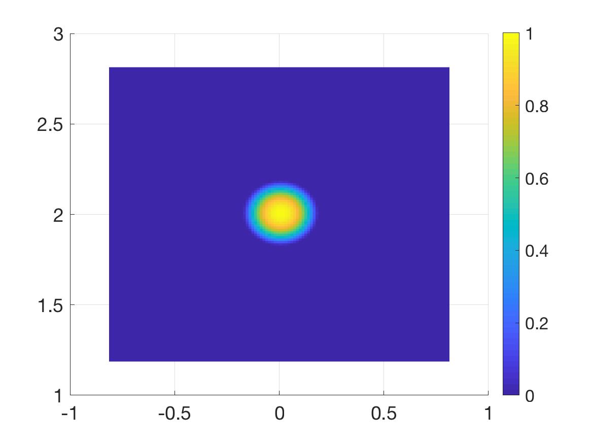
   (a) The true function $f^{*}$

   

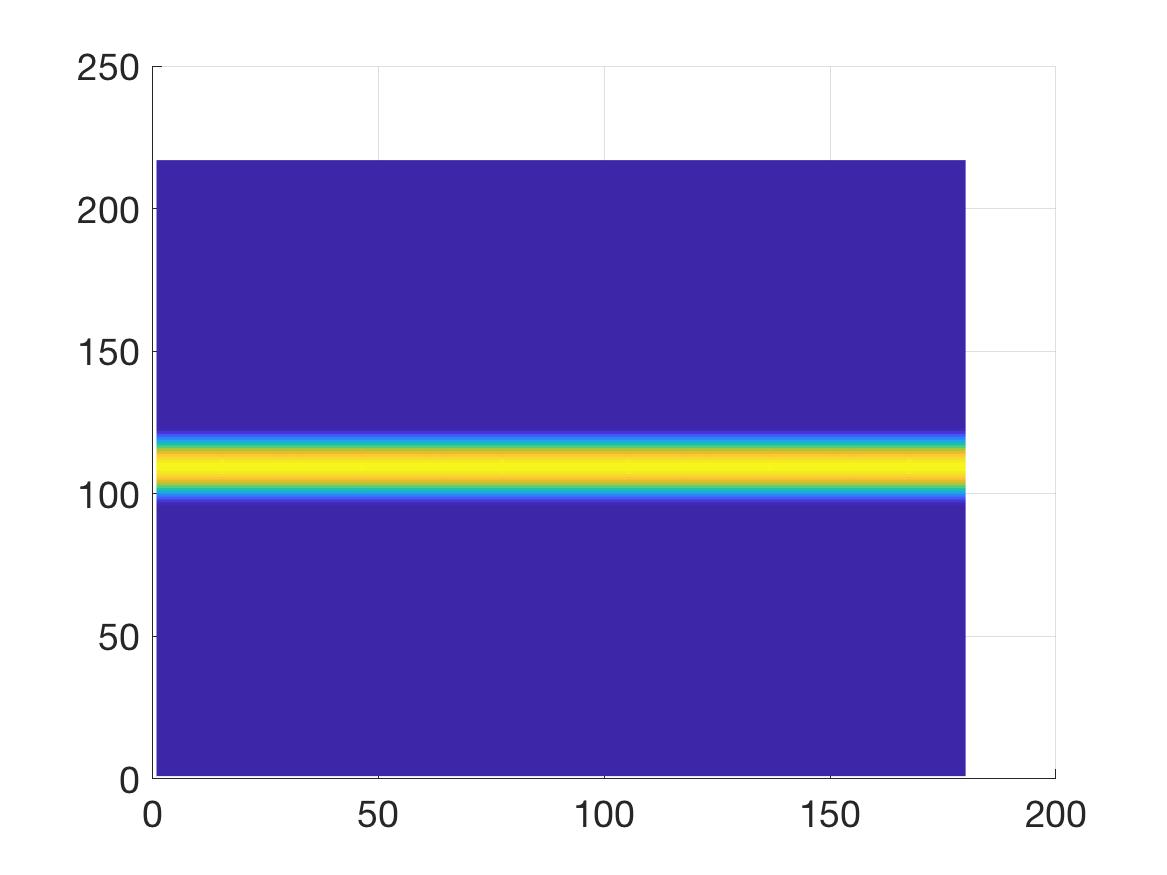
   (b) The Radon transform of $f^{*}$ computed by the function “radon” of Matlab

   

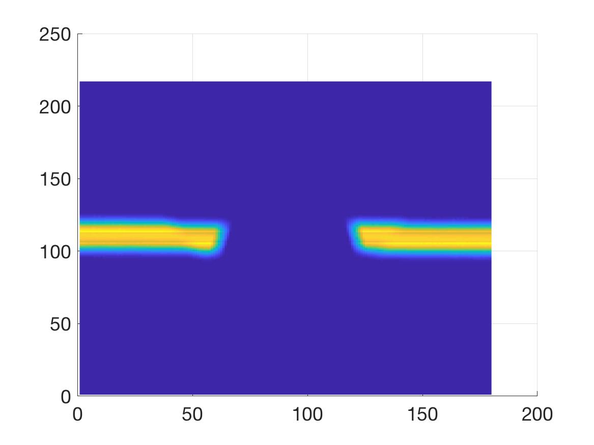
   (c) The incomplete tomographic data with $5\%$ noise

   

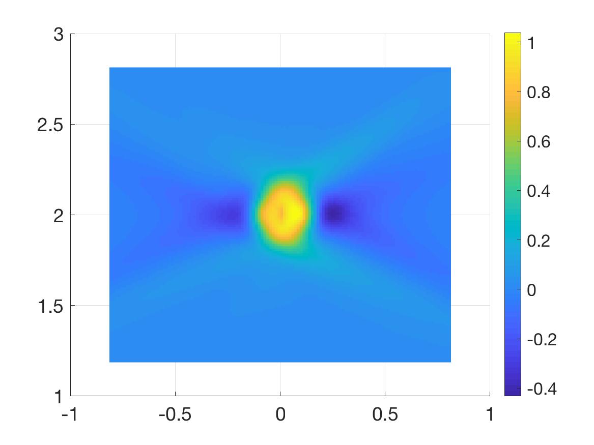
   (d) The function $f_{\rm comp}^{\rm iradon}$ computed by the filtered back projection algorithm, noise level $5\%$

   

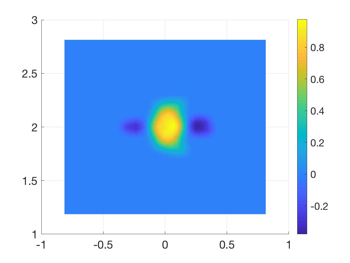
   (e) The function $f_{\rm comp}^{\rm iradon}$ computed by the filtered back projection algorithm, noise level $5\%$, together with the post processing of Section 5.4

   

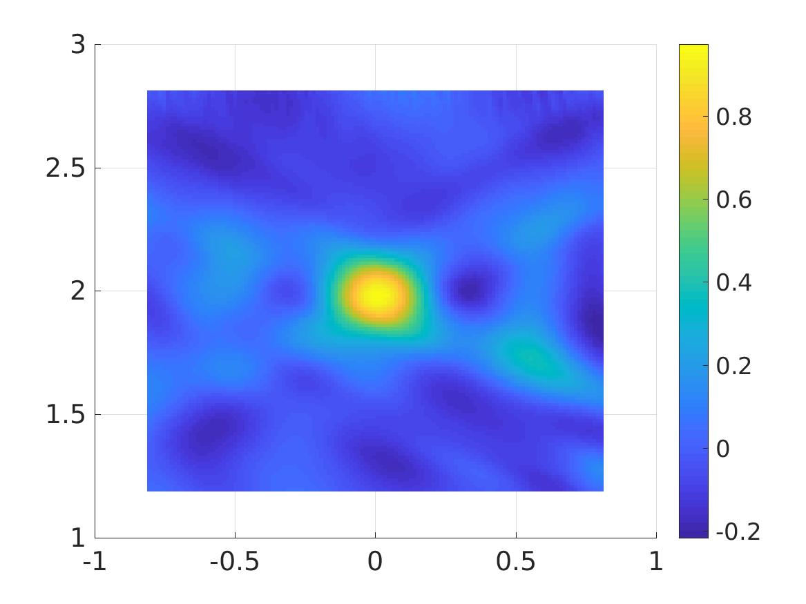
   (f) The function $f_{\rm comp}$ by our method in Section 5.2, noise level $5\%$

   

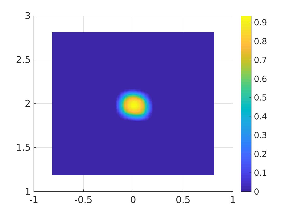
   (g) The function $f_{\rm comp}$ by our method in Section 5.2, noise level $5\%$, together withpost processing of Section 5.4

   

   (h) The function $f_{\rm comp}$ by our method in Section 5.2, noise level $15\%$

   

   (i) The function $f_{\rm comp}$ by our method in Section 5.2, noise level $15\%$, post processing of Section 5.4

   Figure 2: Test 1, inclusion number 1. The data and the reconstructions of the function $f^{\ast}.$ One can see from (e),(g),(i) that the image quality provided by our method is slightly better than that of the filtered back projection method.

2. Test 2. In this case, we set $\Omega=(-1,1)\times(3,5)$. The distance between the source line $\Gamma_{d}$ and the domain $\Omega$ is 3, which is three times larger than the distance in test 1. The true function $f^{\ast}$ is

   $$f^{\ast}(\mathbf{x})=-6\varphi((\mathbf{x}-\mathbf{x}_{1})/r_{1})+5\varphi((\mathbf{x}-\mathbf{x}_{2})/r_{2})+6\varphi((\mathbf{x}-\mathbf{x}_{3})/r_{3})$$

   where $\mathbf{x}_{1}=(-0.4,4),r_{1}=0.2$, $\mathbf{x}_{2}=(-0.1,3.57),r_{2}=0.23$, $\mathbf{x}_{3}=(0.4,4)$ and $r_{3}=0.18.$ Hence, we have here three different radii of circles varying between 0.18 and 0.23. We note that $f\left(\mathbf{x}\right)\leq 0$ inside of the first circle, and $f\left(\mathbf{x}\right)\geq 0$ inside of second and third circles. We number these inclusions as “inclusions number 1, 2 and 3” respectively. The true and reconstructed functions $f$ are displayed in Figure 3.

   

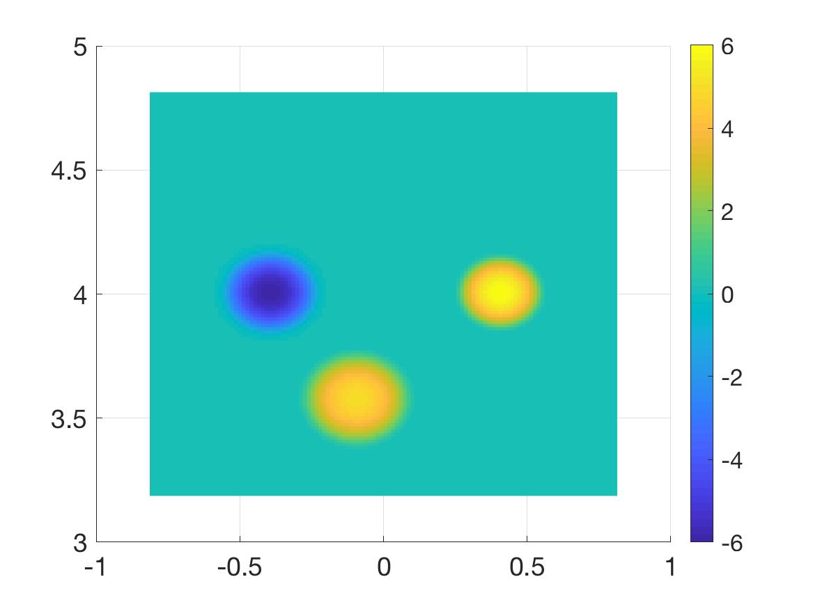
   (a) The true function $f^{*}$

   

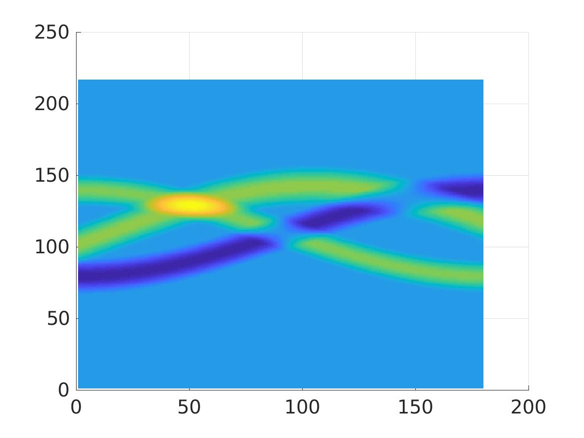
   (b) The Radon transform of $f^{*}$ computed by the function “radon” of Matlab

   

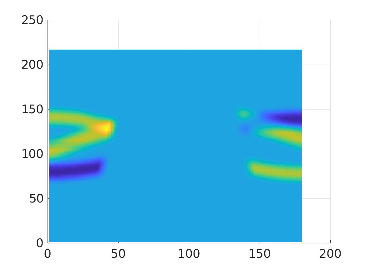
   (c) The incomplete tomographic data with $5\%$ noise

   

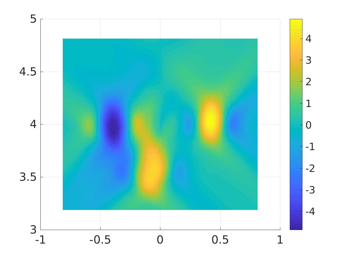
   (d) The function $f_{\rm comp}^{\rm iradon}$ computed by the filtered back projection algorithm, noise level $5\%$

   

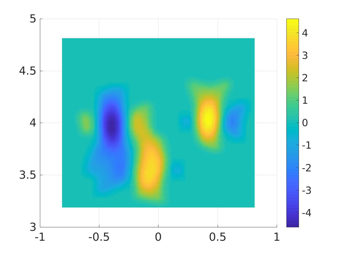
   (e) The function $f_{\rm comp}^{\rm iradon}$ computed by the filtered back projection algorithm, noise level $5\%$, together with the post processing of Section 5.4

   

   (f) The function $f_{\rm comp}$ by our method in Section 5.2, noise level $5\%$

   

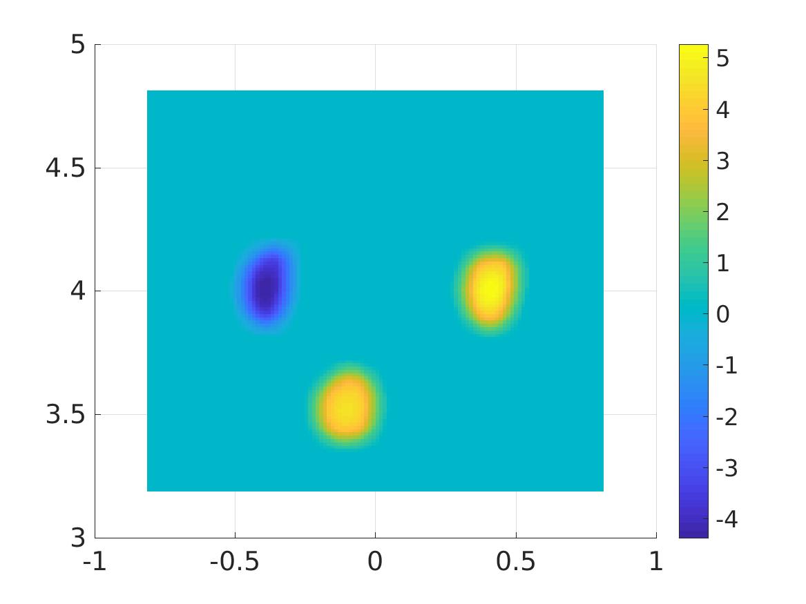
   (g) The function $f_{\rm comp}$ by our method in Section 5.2, noise level $5\%$, together withpost processing of Section 5.4

   

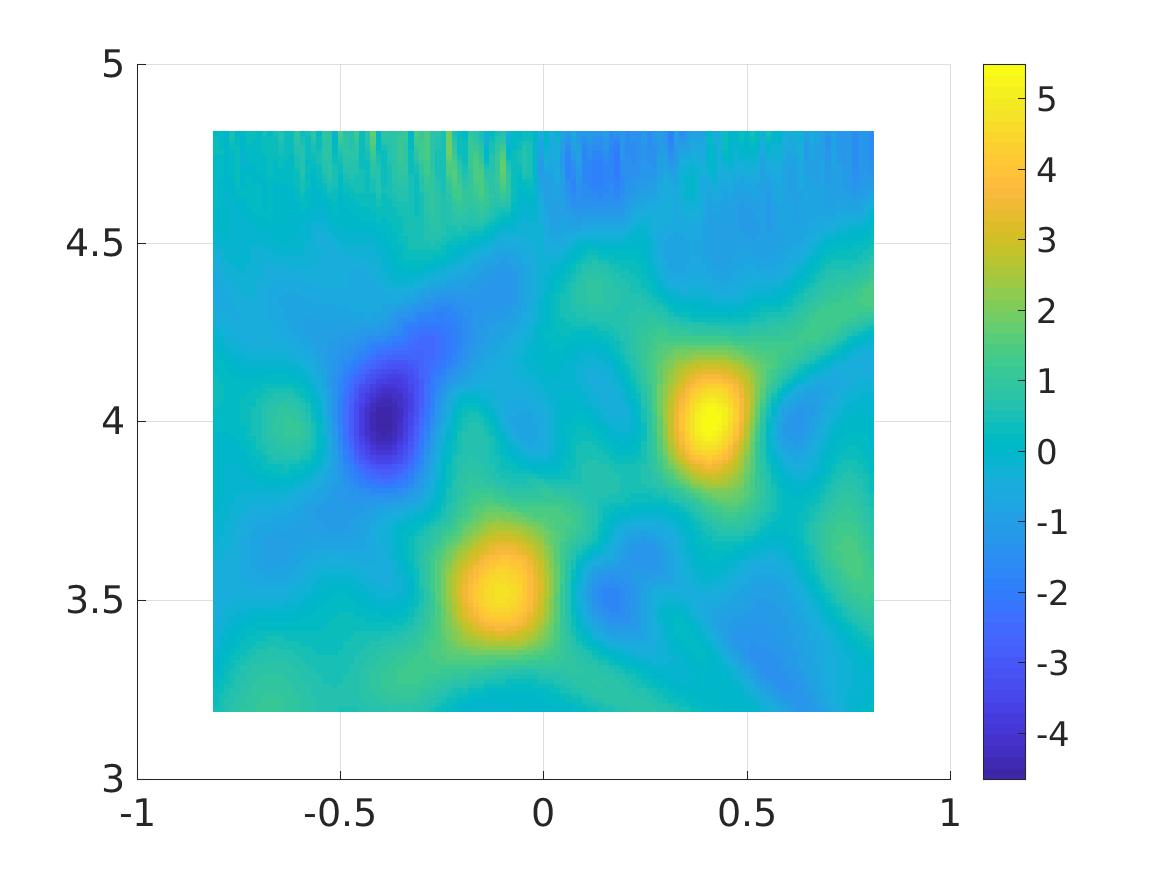
   (h) The function $f_{\rm comp}$ by our method in Section 5.2, noise level $15\%$

   

   (i) The function $f_{\rm comp}$ by our method in Section 5.2, noise level $15\%$, post processing of Section 5.4

   Figure 3: Test 2. The data and the reconstructions of the function $f^{\ast}$ in the case of three inclusions. On (a),(d)-(i) inclusions from left to right are numbered as 2,3 and 4. One can see from (e),(g),(i) that the image quality provided by our method is better than that of the filtered back projection method.

3. Test 3. Next, we test a non smooth function and the inclusion whose shape is not circular. Set $\Omega=(-1,1)\times(3.5,5.5).$ The distance between the source line $\Gamma_{d}$ and the domain $\Omega$ is now 3.5, which is greater than in previous two tests. The true function $f^{\ast}$ is

   $$f^{\ast}(\mathbf{x})=\chi_{\{\mathbf{x}=(x,y):0.3<|x|+|y-4.5|<0.6,x>0.3,y>4.5\}},$$

   where $\chi$ is the characteristic function. The image of the true inclusion looks like a letter $L$ rotated clockwise by $3\pi/4$ around the center of $\Omega$. The true and reconstructed functions $f$ are displayed in Figure 4.

   

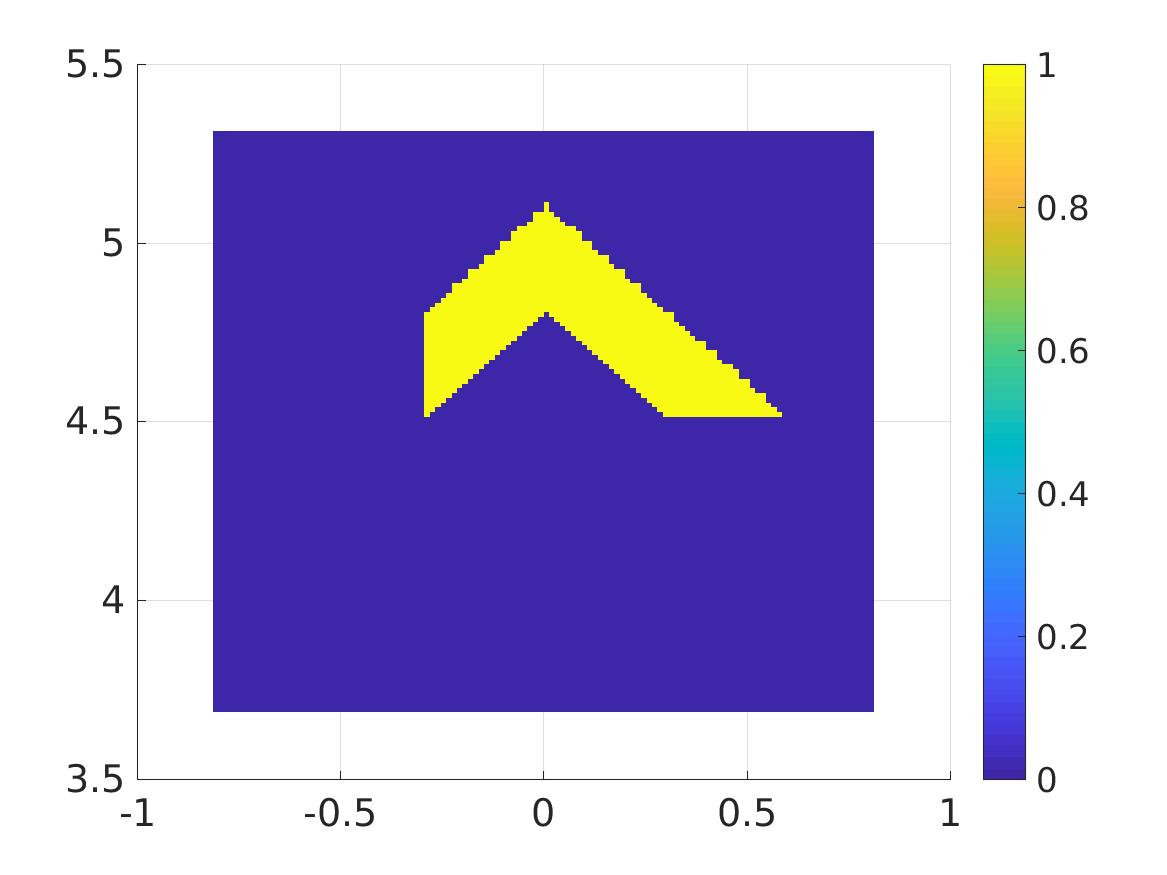
   (a) The true function $f^{*}$

   

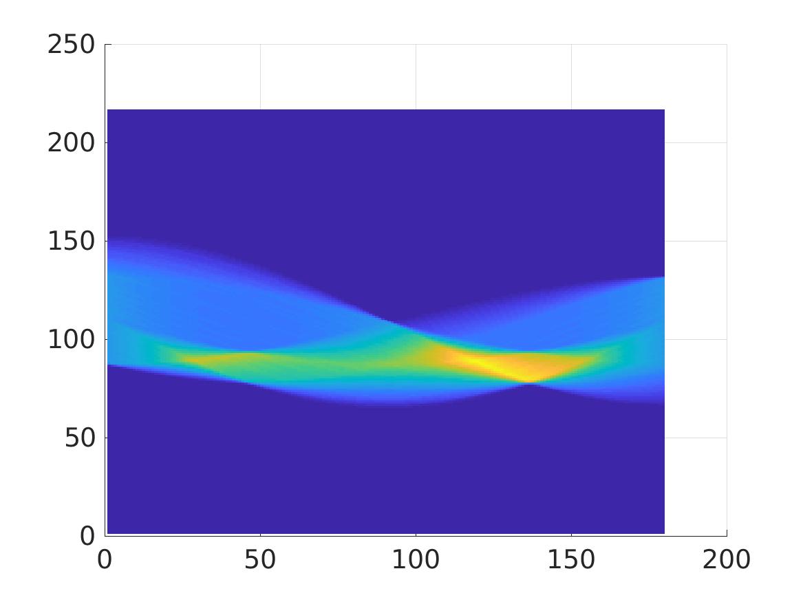
   (b) The Radon transform of $f^{*}$ computed by the function “radon” of Matlab

   

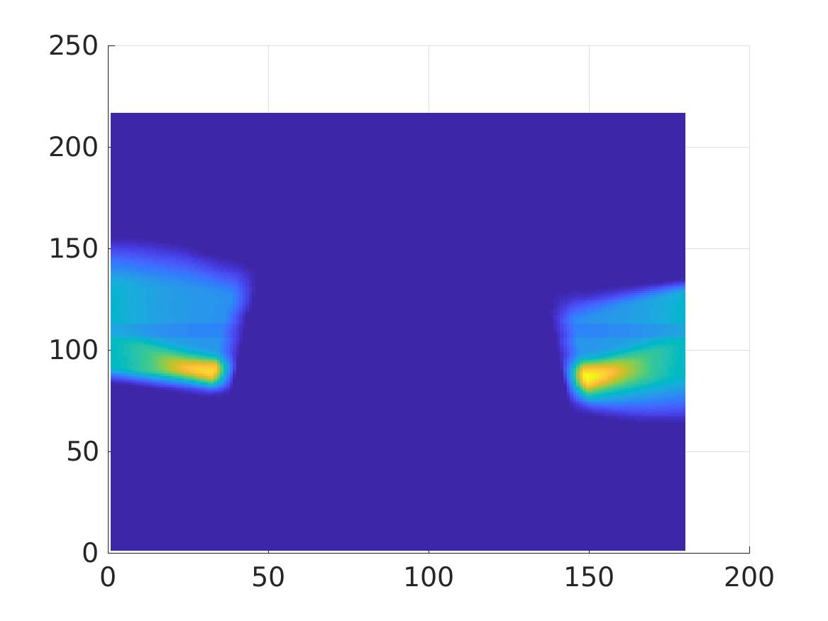
   (c) The incomplete tomographic data with $5\%$ noise

   

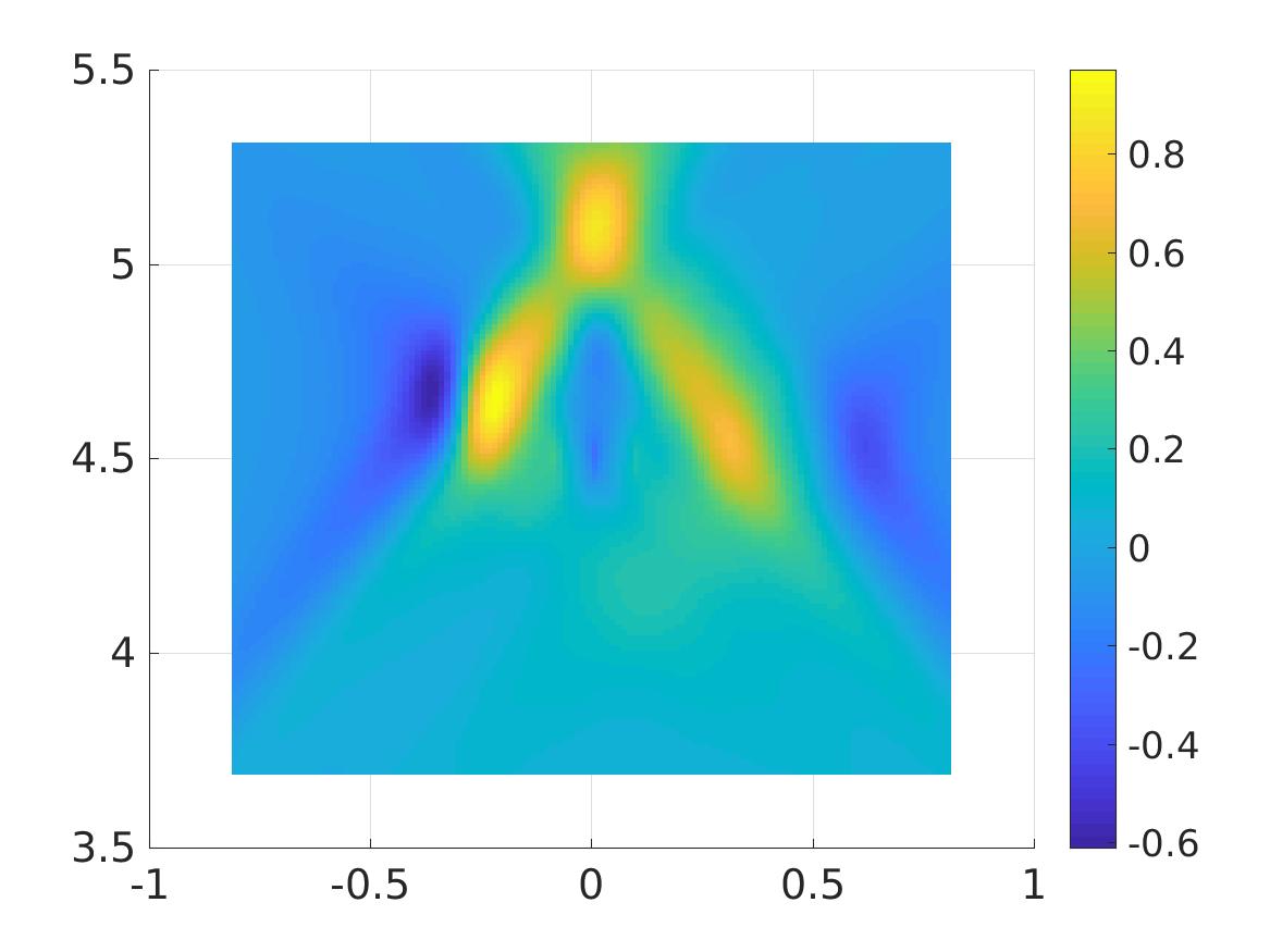
   (d) The function $f_{\rm comp}^{\rm iradon}$ computed by the filtered back projection algorithm, noise level $5\%$

   

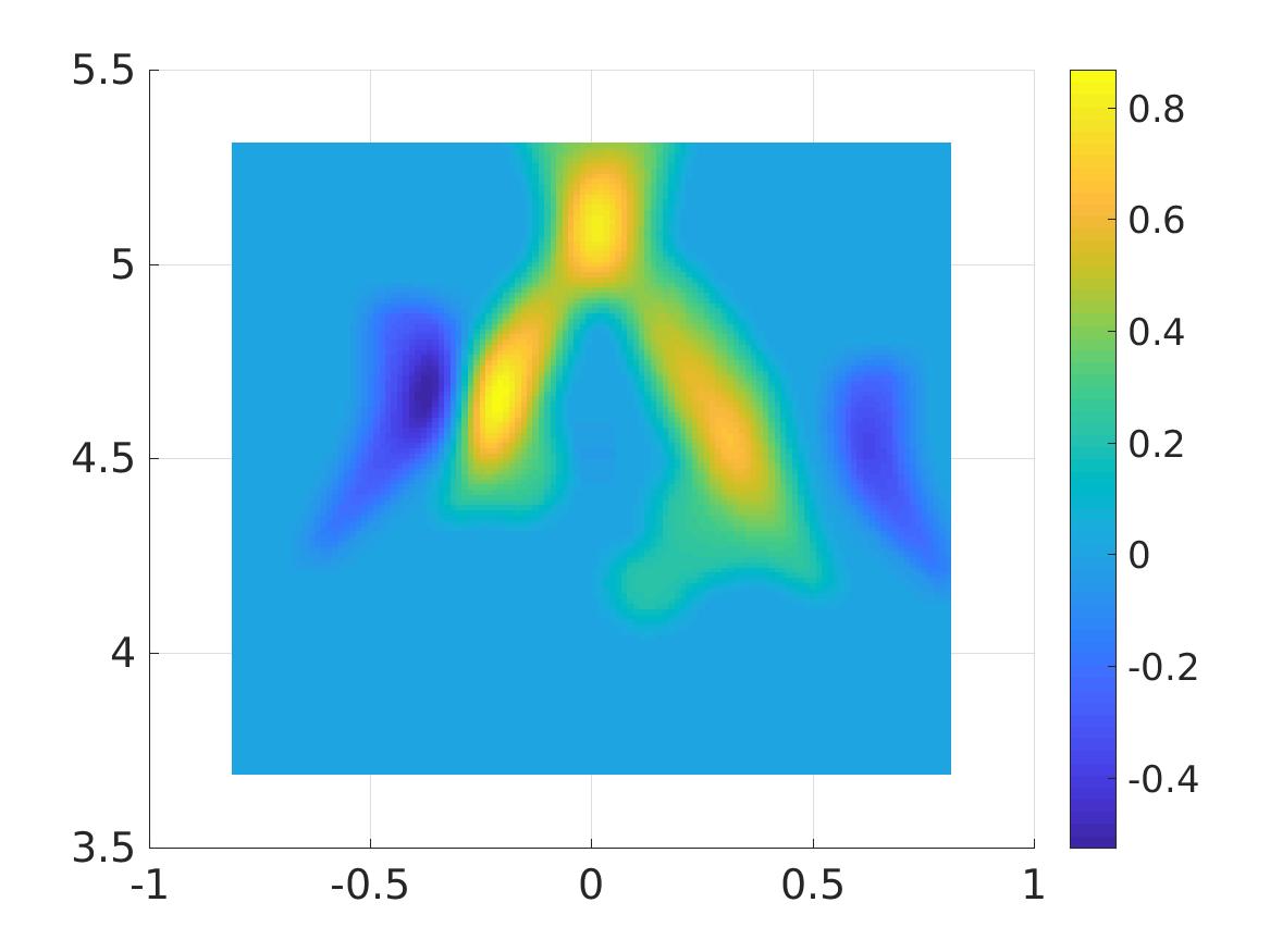
   (e) The function $f_{\rm comp}^{\rm iradon}$ computed by the filtered back projection algorithm, noise level $5\%$, together with the artifact remover

   

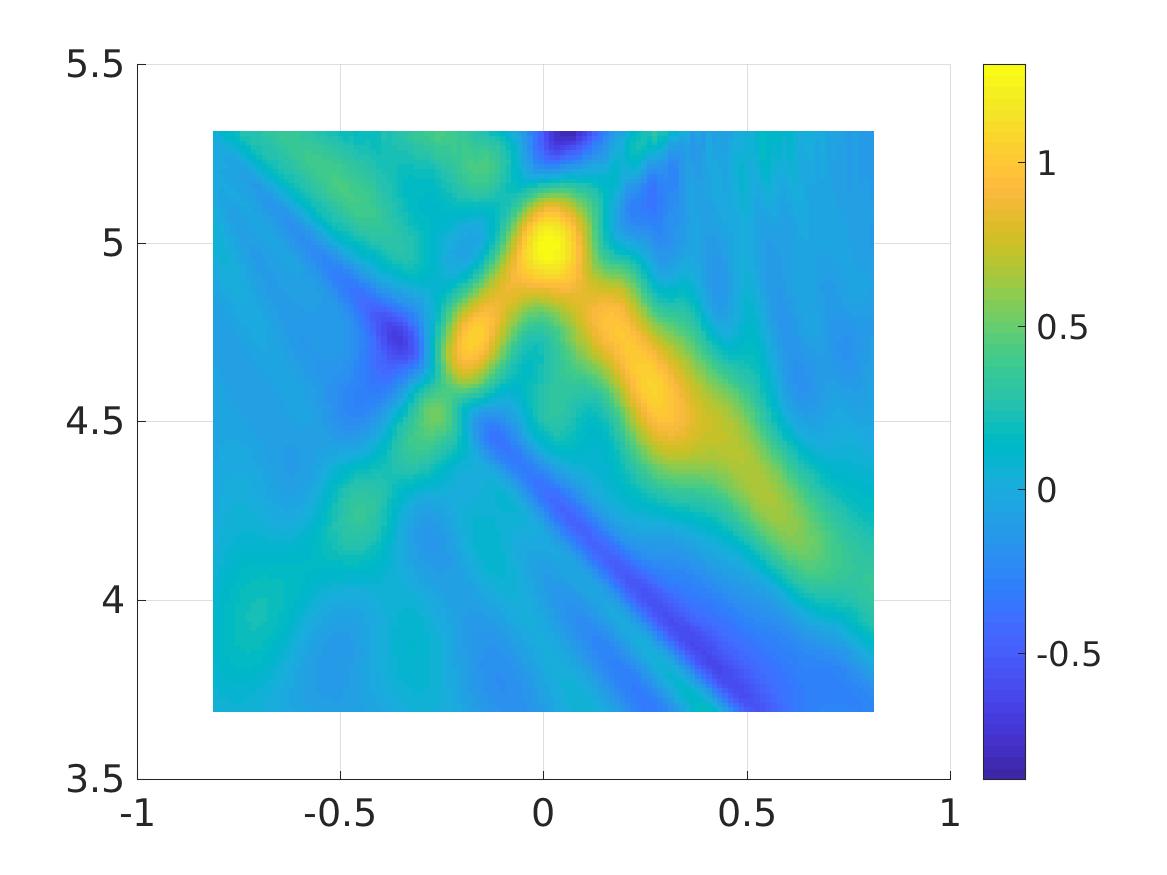
   (f) The function $f_{\rm comp}$ by our method in Section 5.2, noise level $5\%$

   

   (g) The function $f_{\rm comp}$ by our method in Section 5.2, noise level $5\%$, together with the artifact remover

   

   (h) The function $f_{\rm comp}$ by our method in Section 5.2, noise level $15\%$

   

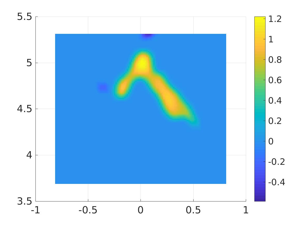
   (i) The function $f_{\rm comp}$ by our method in Section 5.2, noise level $15\%$, together with the artifact remover

   Figure 4: Test 3. The data and the reconstructions of the non smooth function $f^{\ast}$ in the case of an $L$-like shape. The shape is well seen on images (g) and (i) which result from our method and it is not seem well on (e), which results from the filtered back projection method. Comparison of (e) with (g) and (i) indicates that the image quality provided by our method is significantly better than that of the filtered back projection method.

4. Test 4. We next test our method with a non smooth function $f^{\ast}$ that is nonzero on a square rotated by $\pi/4$ around the center of $\Omega.$ This square has two positive sides and two negative sides. In particular, we want to see whether or not our method can detect a void inside of a square.

   The domain $\Omega$ is set to be $\Omega=(-1,1)\times(3.5,5.5),$ just as in the previous numerical test. The function $f^{\ast}$ is given by

   $$f^{\ast}(\mathbf{x})=\chi_{\{\mathbf{x}=(x,y):0.3<|x|+|y-4.5|<0.6,y>4.5\}}\\ -\chi_{\{\mathbf{x}=(x,y):0.3<|x|+|y-4.5|<0.6,y<4.5\}}.$$

   The true and reconstructed functions $f$ are displayed in Figure 5.

   

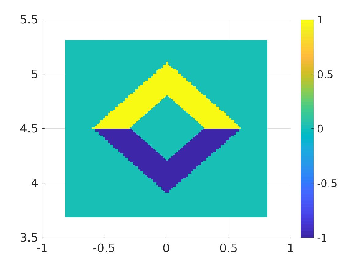
   (a) The true function $f^{*}$

   

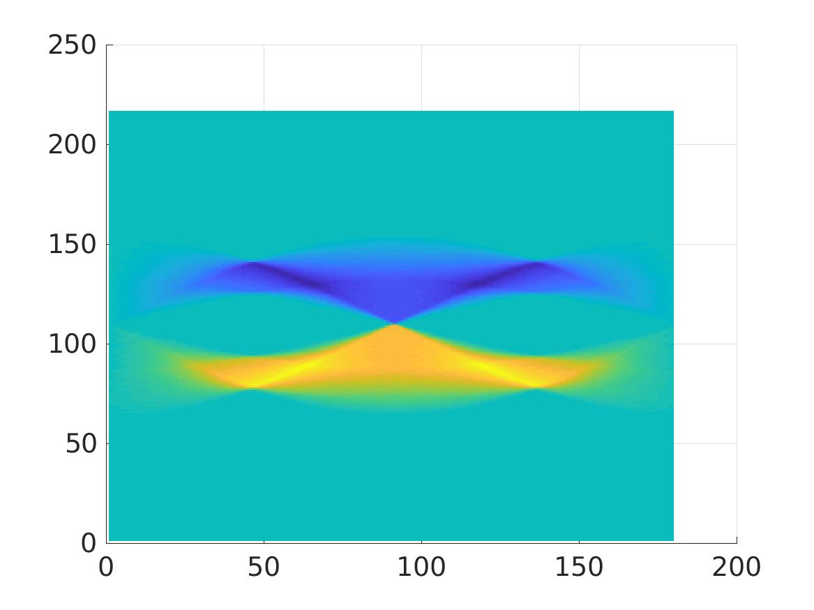
   (b) The Radon transform of $f^{*}$ computed by the function “radon” of Matlab

   

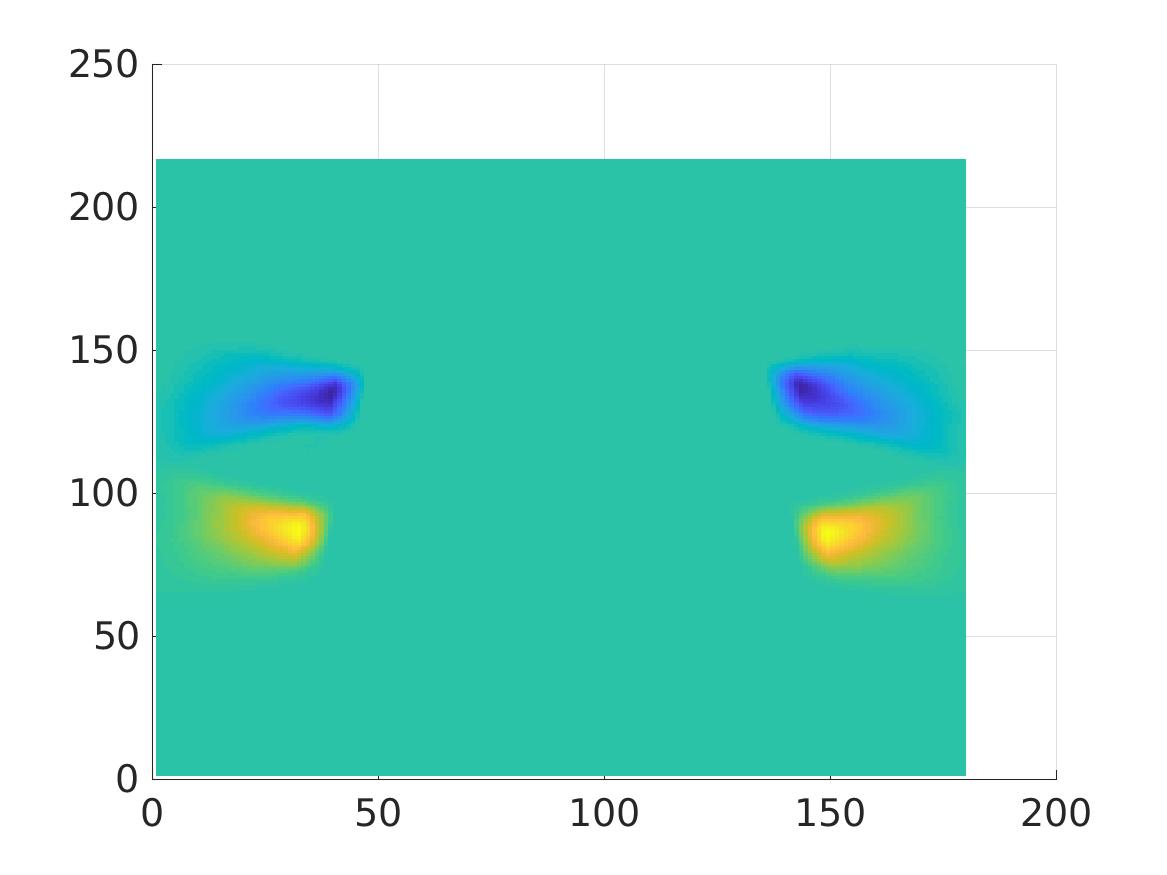
   (c) The incomplete tomographic data with $5\%$ noise

   

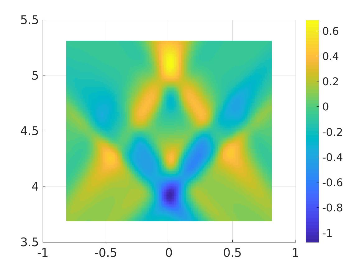
   (d) The function $f_{\rm comp}^{\rm iradon}$ computed by the filtered back projection algorithm, noise level $5\%$

   

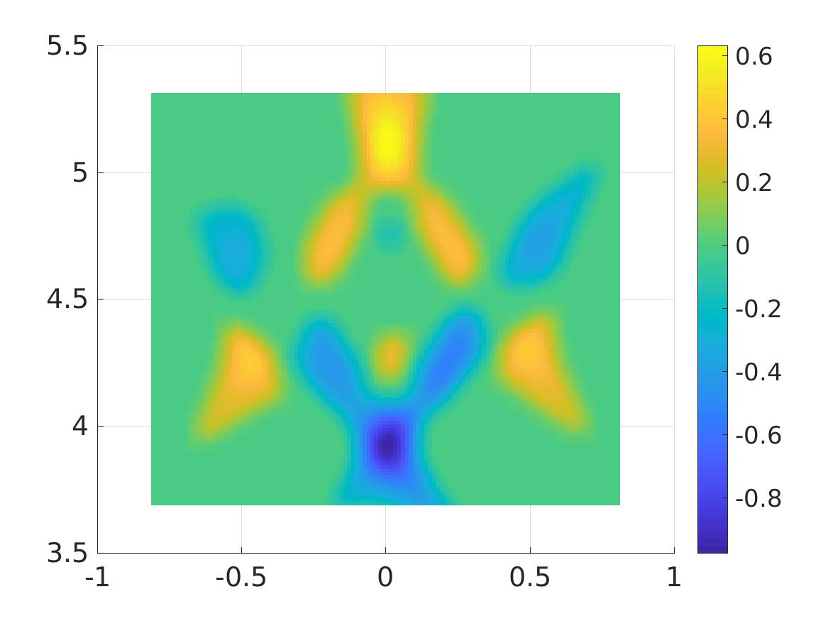
   (e) The function $f_{\rm comp}^{\rm iradon}$ computed by the filtered back projection algorithm, noise level $5\%$, together with the post processing of Section 5.4

   

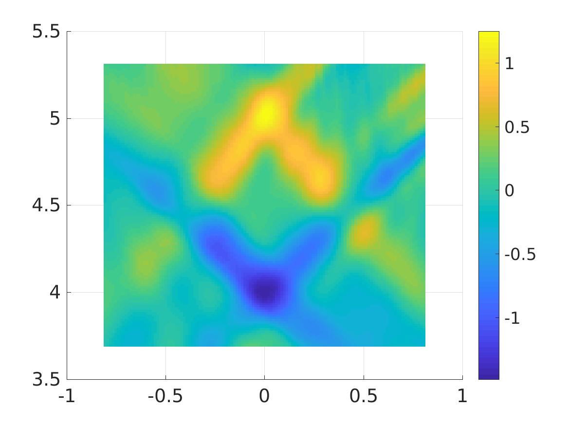
   (f) The function $f_{\rm comp}$ by our method in Section 5.2, noise level $5\%$

   

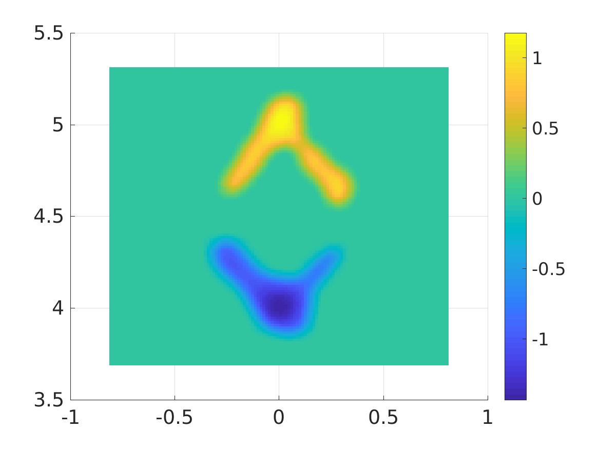
   (g) The function $f_{\rm comp}$ by our method in Section 5.2, noise level $5\%$, together withpost processing of Section 5.4

   

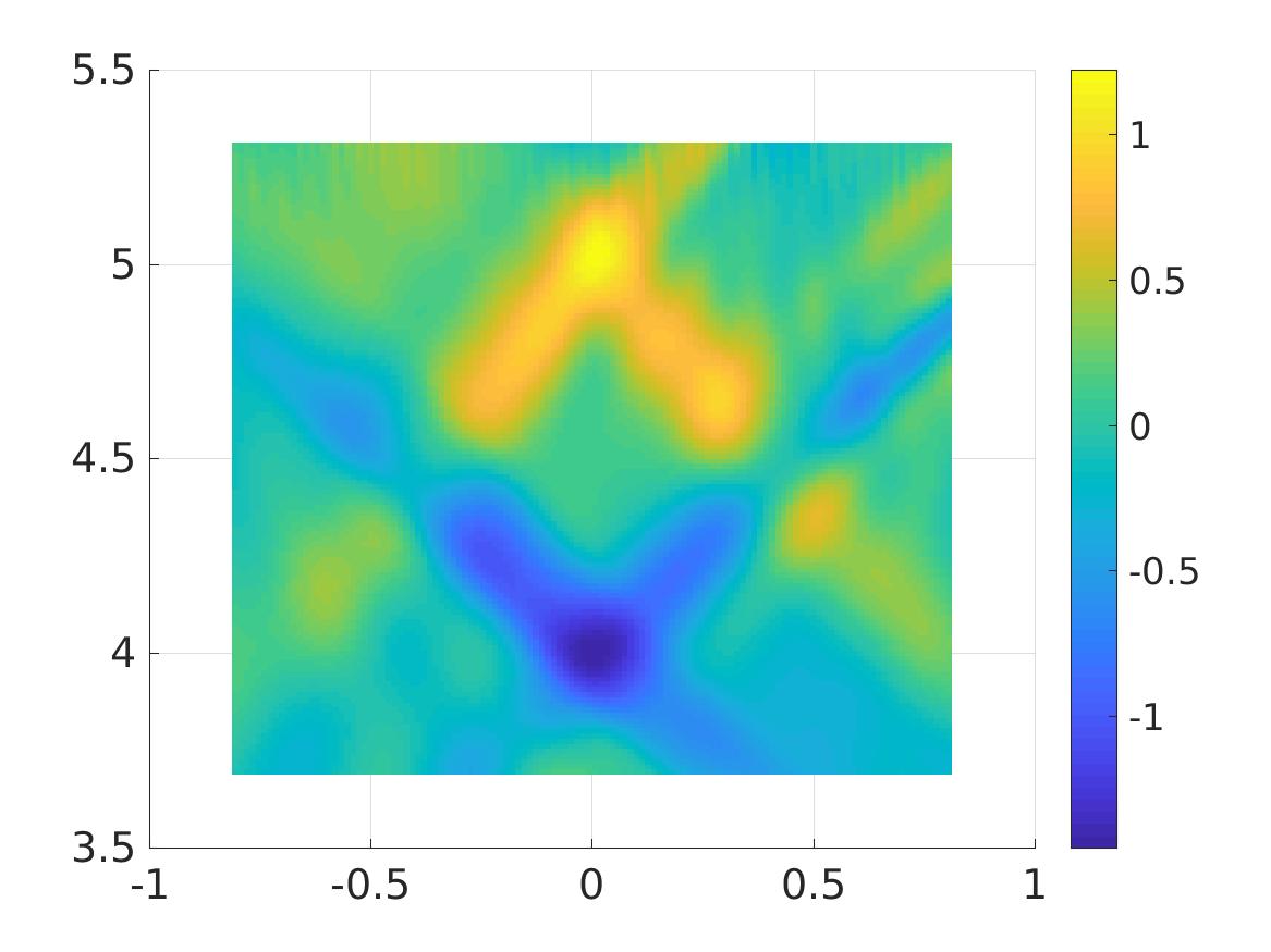
   (h) The function $f_{\rm comp}$ by our method in Section 5.2, noise level $15\%$

   

   (i) The function $f_{\rm comp}$ by our method in Section 5.2, noise level $15\%$, post processing of Section 5.4

   Figure 5: Test 4. The data and the reconstructions of the non smooth function $f^{\ast}$ in the case of a square shape. The shape is satisfactory on (g) and (i) and the void is clearly seen on them, whereas (e) is less clear. Comparing of (e) with (g) and (i), one can see that the image quality provided by our method is significantly better than that of the filtered back projection method.

One can see from these figures that our method is quite stable with respect to the noise. In fact, the reconstructed errors and images do not change much when the noise increases from $5\%$ to $15\%$.

Remark 6.1 (The comparison of artifacts).

Comparing Figures 2e–5e versus Figures 2g–5g and Figures 2i–5i, we observe that the unwanted artifacts involved in the results by the filtered back projection method are much stronger than the ones in the numerical reconstructions obtained by our method. More precisely, the “$20\%$ filter” in (5.15) cannot remove unwanted artifacts in $f_{\mathrm{comp}}^{\mathrm{iradon}}$ while it works well for the artifacts in $f_{\mathrm{comp}}$ obtained by using our method.

It seems to be on the first glance that the longer the source line $\Gamma_{d}$ in (2.2) is, the wider is the angle to “see” the inclusions. However, in computation, there is a limiting length $2d_{\lim}$ for $\Gamma_{d}$ such that our method fails for $d>d_{\lim}.$ For example, for parameters $a$ and $b$ used in Tests 1 and 2, this limiting length is $d_{\lim}=14$. To explain this length limitation, we observe that a more detailed analysis of formulae (3.6), (3.8) and Lemma 3.3 shows that one should have in Lemma 3.15 $\left(R+d\right)/a_{0}^{2}\ll 1.$ The fact that this inequality is not exactly satisfied in Tests 1-4 can be viewed as another indication of the stability of our technique. However, this inequality is violated at large for $d\geq 14,$ and this is why our method fails to work for such values of $d$.

6.1 Reconstruction errors

As to the image quality, the visual analysis of Figures 2(e),(g),(i)-5(e),(g),(i) indicates that, at least in our four tests, our method provides better quality images than the filtered back projection method. Furthermore, the difference of those qualities increases in the favor of our method as the structures of inclusions become more complicated.

We now discuss the reconstructed errors of the numerical solutions only in the first two tests in which true function $f^{\ast}$ involves inclusions. Satisfactory reconstructed values were obtained, see Table 1 and Figure 6. We do not present the error estimates for Tests 3 and 4 since it is not clear for us how to define the values of the reconstructed functions for the kinds of non-convex inclusions in those two tests. However, it can be seen from Figures 4e, 4g, 4i, 5e, 5g and 5i and the enclosed color bars that the reconstructions of the function $f$ are acceptable.

Table 1: Correct and computed inclusions in Tests 1 and 2. Here, FBP means filtered back projection, Nm means inclusion number (see descriptions of Tests 1,2), $f_{\mathrm{true}}$ is the extreme value of the true function $f^{*}$ in the inclusion, loc_true means true location where the extreme value of $f^{*}$ occurs, $f_{\mathrm{comp}}$ is the extreme value of the computed function $f_{\mathrm{comp}}$ in the inclusion, and loc_true means true location where the extreme value of $f_{\mathrm{comp}}$ occurs.

Inc. Nm	loctrue	$f_{\mathrm{true}}$	Method	noise level	loccomp	$f_{\mathrm{comp}}$
1	(0.0, 2)	1	FBP method	5%	(0.053, 2.000)	0.9751
1	(0.0, 2)	1	Our method	5%	(0.000, 1.973)	0.9781
1	(0.0, 2)	1	Our method	15%	(0.013, 1.973)	0.9361
2	(-0.4, 4)	-6	FBP method	5%	(-0.400, 3.960)	-4.644,
2	(-0.4, 4)	-6	Our method	5%	(-0.4, 4)	-4.373
2	(-0.4, 4)	-6	Our method	15%	(-0.4, 4)	-4.378
3	(-0.1, 3.5714)	5	FBP method	5%	(-0.067, 3.560)	3.829
3	(-0.1, 3.5714)	5	Our method	5%	(-0.107, 3.507),	4.615
3	(-0.1, 3.5714)	5	Our method	15%	(-0.107, 3.52)	4.574
4	(0.4, 4)	6	FBP method	5%	(0.413, 4.027)	4.617
4	(0.4, 4)	6	Our method	5%	(0.4, 4)	5.261
4	(0.4, 4)	6	Our method	15%	(0.4, 4)	5.16

We now analyze Figure 6. In this figure “absolute errors in locations of reconstructed inclusions” means errors at points where the reconstructed function $f$ achieves its extreme value, for each inclusion of Tests 1,2. One can see from Figure 6(a) that, in terms of locations, our method performs better than the filtered back projection method for inclusions 1,2 and 4. And it performs worse for inclusion number 3. As to Figure 6(b), one can observe that our method provides more accurate extreme values for inclusions 3 and 4. In the case of inclusion 1, the accuracy in calculating extreme values is about the same for both methods for the case of 5% noise. In the case of inclusion 2, the accuracy in calculating the extreme value is better for filtered back projection method.

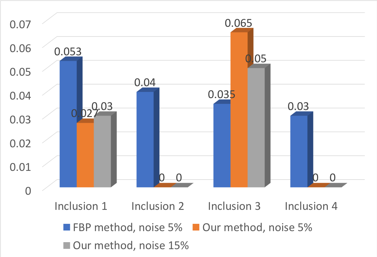
(a) Absolute errors in locations of reconstructed inclusions. In spite of noise, the reconstructed locations of inclusions 2 and 4 are exact.

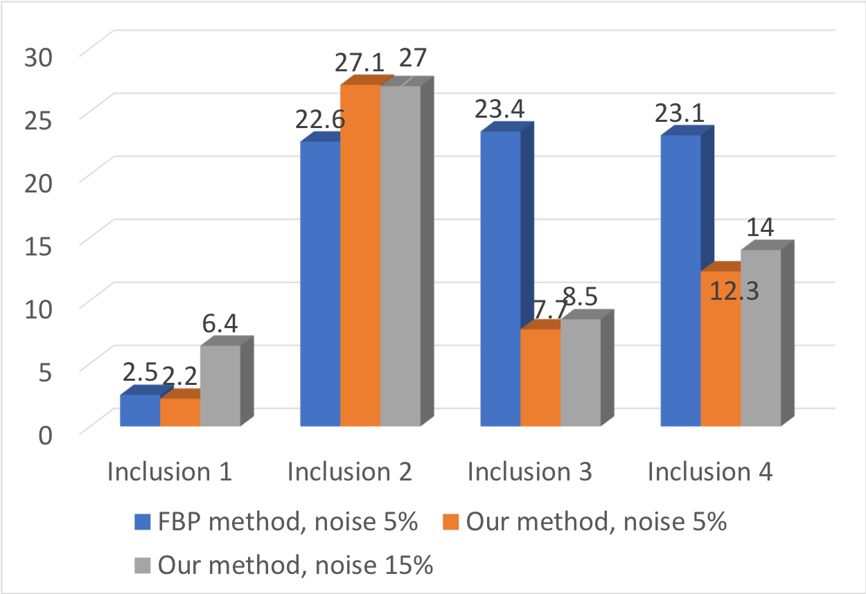
(b) Relative errors (in %) of the extreme value of the reconstructed function $f_{\rm comp}$ in four inclusions in Tests 1 and 2.

Figure 6: Comparison of reconstruction errors of our method with filtered back projection method for Tests 1 and 2, see their descriptions as well as Figures 2 and 3 for numbering of inclusions. a) Absolute errors in locations of points with extreme values of the function $f$. b) Relative errors (in %) of the reconstructed extreme values of the function f inside the inclusions.

7 Concluding Remarks

While all current techniques of the inversion of the data for the X-ray tomography are based on some inversion formulae, we have proposed a new numerical method here, which does not intend to obtain an inversion formula. Instead, it uses a well known transport PDE governing propagation of X-rays. Our method works for a special case of a limited angle data, which might be potentially applied to, e.g. checking out bulky luggage in airports and checking out quality of walls in houses. Using the original idea of the method of [10] as well as a recently introduced new orthonormal basis in $L^{2}\left(-d,d\right)$ [23], we obtain a system of coupled first order PDEs in which the target function $f$ is not involved. The boundary value problem for this system is over determined. Therefore, we solve this boundary value problem by the quasi-reversibility method, which is perfectly suited for solutions of overdetermined boundary value problems for PDEs. We prove a new Carleman estimate and use it then to prove uniqueness and existence of the solution for the quasi-reversibility method. Next, the same Carleman estimate enables us to establish convergence rate of regularized solutions. We work with a semi discrete version of the quasi-reversibility method, which is more realistic than its conventional continuos version, see a survey in [21] for the continuos version.

We have conducted numerical testing of this new method for noisy data, including comparison with the filtered back projection method for Radon transform. In the latter we have heuristically assigned zero to the missing data, similarly with [5]. We point out that this assignment cannot be rigorously justified for the filtered back projection method, unlike our method. We have observed that our method sustains 5% and 15% of noise and resulting images are about the same.

The visual analysis indicates that, at least in the above Tests 1-4, images resulting from our method have a better quality than those provided by the filtered back projection method. Also, the more complicated the structures of inclusions are, the larger in the favor of our method is the difference of qualities of those images. It can be seen from Table 1 that our method also provides more accurate locations of imaged targets for Tests 1,2 for three (3) out of four (4) inclusions. As to the extreme values of the function $f$ inside of inclusions, it can be seen from Table 1 that our method provides about the same accuracy as the filtered back projection method for one inclusion (number 1), better accuracy for two (number 3,4) and worse accuracy for one inclusion (number 2), also see Figure 6. Comparison in numbers for Tests 3,4 is hard to provide due to the complicated structures of inclusions in these tests.

Finally, we observe that, in the case of the attenuated X-ray transform [29], the following analog of PDE (3.1) is valid [14]:

(7.1) $$\frac{x-\alpha}{\sqrt{\left(x-\alpha\right)^{2}+y^{2}}}u_{x}+\frac{y}{\sqrt{\left(x-\alpha\right)^{2}+y^{2}}}u_{y}+c\left(x,y\right)u=f\left(x,y\right),\quad(x,y)\in\Omega$$

with an appropriate function $c\left(x,y\right)$. This equation differs from equation (3.1) by the term $c\left(x,y\right)u.$ Since this is the lower order term in PDE (7.1) and since Carleman estimates are “sensitive” only to the principal parts of PDE operators and “non sensitive” to their lower terms, then a slight modification of our technique works for this case. Numerical studies of this problem are outside of the scope of the current publication. We refer to [33] for an inversion formula for the attenuated X-ray transform.

References

- [1] L. L. Barannyk, J. Frikel and L. V. Nguyen, On artifacts in limited data spherical radon transform: curved observation surface, Inverse Problems, 32 (2016), p. 015012.
- [2] E. Bécache, L. Bourgeois, L. Franceschini, and J. Dardé, Application of mixed formulations of quasi-reversibility to solve ill-posed problems for heat and wave equations: The 1d case, Inverse Problems & Imaging, 9 (2015), pp. 971–1002.
- [3] L. Beilina and M.V. Klibanov, Approximate Global Convergence and Adaptivity for Coefficient Inverse Problems, Springer, New York, 2012.
- [4] M. Bellassoued and M. Yamamoto, Carleman Estimates and Applications to Inverse Problems for Hyperbolic Systems, Springer, Japan, 2017.
- [5] L. Borg, J. Frikel, J. S. Jrgensen, and E. T. Quinto, Full characterization of reconstruction artifacts from arbitrary incomplete x-ray ct data, Arxiv:1707.03055v3, (2018).
- [6] L. Borg, J. S. Jrgensen, J. Frikel, and J. Sporring, Reduction of variable-truncation artifacts from beam occlusion during in situ X-ray tomography, Meas. Sci. Tech., 28 (2017), p. 19pp.
- [7] L. Borg, J. S. Jrgensen, and J. Sporring, Towards characterizing and reducing artifacts caused by varying projection truncation, tech. rep., Department of Computer Science, University of Copenhagen, 2017/1.
- [8] L. Borg, J. S. Jrgensen, and J. Sporring, Convergence rates for the quasi-reversibility method to solve the Cauchy problem for Laplace’s equation, Inverse Problems, 22 (2006), pp. 413–430.
- [9] L. Bourgeois and J. Dardé, A duality-based method of quasi-reversibility to solve the Cauchy problem in the presence of noisy data, Inverse Problems, 26 (2010), p. 095016.
- [10] A. Bukhgeim and M. Klibanov, Uniqueness in the large of a class of multidimensional inverse problems, Soviet Math. Doklady, 17 (1981), pp. 244-247.
- [11] C. Clason and M. V. Klibanov, The quasi-reversibility method for thermoacoustic tomography in a heterogeneous medium, SIAM J. Sci. Comput., 30 (2007), pp. 1–23.
- [12] J. Dardé, Iterated quasi-reversibility method applied to elliptic and parabolic data completion problems, Inverse Problems and Imaging, 10 (2016), pp. 379–407.
- [13] J. Frikel and E. T. Quinto, Characterization and reduction of artifacts in limited angle tomography, Inverse Problems, 29 (2013), p. 125007.
- [14] A. H. Hasanoğlu and V. G. Romanov, Introduction to Inverse Problems for Differential Equations, Springer, Cham, 2017.
- [15] S.I. Kabanikhin, A. D. Satybaev and M.A. Shishlenin, Direct Methods of Solving Inverse Hyperbolic Problems, VSP, The Netherlands, 2005.
- [16] S.I. Kabanikhin and M.A. Shishlenin, Numerical algorithm for two-dimensional inverse acoustic problem based on Gel’fand–Levitan–Krein equation, J. Inverse and Ill-Posed Problems, 18 (2011), 979-995.
- [17] S.I. Kabanikhin, K.K. Sabelfeld, N.S. Novikov and M.A. Shishlenin, Numerical solution of the multidimensional Gelfand–Levitan equation, J. Inverse and Ill-Posed Problems, 23 (2015), 439-450.
- [18] M.V. Klibanov and F. Santosa, A computational quasi-reversibility method for Cauchy problems for Laplace’s equation, SIAM J. Appl. Math. 51 (1991), pp. 1653–1675.
- [19] M.V. Klibanov and A. Timonov, Carleman Estimates for Coefficient Inverse Problems and Numerical Applications, VSP, Utrecht, 2004.
- [20] M. V. Klibanov, Carleman estimates for global uniqueness, stability and numerical methods for coefficient inverse problems, J. Inverse and Ill-Posed Problems, 21 (2013), pp. 477–560.
- [21] M.V. Klibanov, Carleman estimates for the regularization of ill-posed Cauchy problems, Applied Numerical Mathematics, 94 (2015), pp. 46–74.
- [22] M. V. Klibanov and N. T. Thành, Recovering dielectric constants of explosives via a globally strictly convex cost functional, SIAM J. Appl. Math., 75 (2015), 518-537.
- [23] M. V. Klibanov, Convexification of restricted Dirichlet to Neumann map, J. Inverse and Ill-Posed Problems, 25 (2017), pp. 669–685.
- [24] M. V. Klibanov, J. Li, and W. Zhang, Electrical impedance tomography with restricted dirichlet-to-neumann map data, 2018, arXiv:1803.11193.
- [25] M. V. Klibanov, A.E. Kolesov, A. Sullivan and L. Nguyen, A new version of the convexification method for a 1-D coefficient inverse problem with experimental data, Inverse Problems, accepted for publication, 2018, a preprint is available at https://doi.org/10.1088/1361-6420/aadbc6.
- [26] M.M. Lavrentiev, V.G. Romanov and S.P. Shishatskii, Ill-Posed Problems of Mathematical Physics and Analysis, American Mathematical Society, Providence, RI, 1986.
- [27] A. K. Louis, Incomplete data problems in x-ray computerized tomography I. Singular value decomposition of the limited angle transform, Numer. Math., 48 (1986), pp. 251–262.
- [28] R. Lattès and J. L. Lions, The Method of Quasireversibility: Applications to Partial Differential Equations, Elsevier, New York, 1969.
- [29] N. Natterer, The mathematics of computerized tomography, Classics in Mathematics. Society for Industrial and Applied Mathematics, New York, 2001.
- [30] L. V. Nguyen, On artifacts in limited data spherical Radon transform: flat observation surfaces, SIAM Journal on Mathematical Analysis, 47 (2015), pp. 2984–3004.
- [31] L. V. Nguyen, On the strength of streak artifacts in filtered back-projection reconstructions for limited angle weighted x-ray transform, J. Fourier Anal. Appl., 23 (2017), pp. 712–728.
- [32] L. H. Nguyen, An inverse source problem for hyperbolic equations and the Lipschitz-like convergence of the quasi-reversibility method, preprint, Arxiv : 1806.03921.
- [33] R.G. Novikov, An inversion formula for the attenuated X-ray transformation, Ark. Mat., 40 (2002), pp. 145-167.
- [34] X. Pan, E. Y. Sidky, and M. Vannier, Why do commercial CT scanners still employ traditional, filtered back- projection for image reconstruction?, Inverse Problems, 25 (2009), p. 123009.
- [35] J. Radon, Über die Bestimmung von Funktionen durch ihre Integralwerte längs gewisser Mannigfaltigkeiten, Berichte Sächsische Akademie der Wissenschaften, Leipzig, Mathematisch-Physikalische Klasse, 69 (1917), pp. 262–277.
- [36] J. Radon, On the determination of functions from their integral values along certain manifolds, IEEE Transactions on Medical Imaging. Translated by P.C. Parks from the original German text, 5 (1986), pp. 170–176.
- [37] A.N. Tikhonov, A.V. Goncharsky, V.V. Stepanov and A.G. Yagola, Numerical Methods for the Solution of Ill-Posed Problems, Kluwer, London, 1995.