Open-world Learning and Application to Product Classification

Abstract.

Classic supervised learning makes the closed-world assumption that the classes seen in testing must have appeared in training. However, this assumption is often violated in real-world applications. For example, in a social media site, new topics emerge constantly and in e-commerce, new categories of products appear daily. A model that cannot detect new/unseen topics or products is hard to function well in such open environments. A desirable model working in such environments must be able to (1) reject examples from unseen classes (not appeared in training) and (2) incrementally learn the new/unseen classes to expand the existing model. This is called open-world learning (OWL). This paper proposes a new OWL method based on meta-learning. The key novelty is that the model maintains only a dynamic set of seen classes that allows new classes to be added or deleted with no need for model re-training. Each class is represented by a small set of training examples. In testing, the meta-classifier only uses the examples of the maintained seen classes (including the newly added classes) on-the-fly for classification and rejection. Experimental results with e-commerce product classification show that the proposed method is highly effective.

1. Introduction

An AI agent working in the real world must be able to recognize the classes of things that it has seen/learned before and detect new things that it has not seen and learn to accommodate the new things. This learning paradigm is called open-world learning (OWL) (Chen and Liu, 2018; Bendale and Boult, 2015; Fei et al., 2016). This is in contrast with the classic supervised learning paradigm which makes the closed-world assumption that the classes seen in testing must have appeared in training. With the ever-changing Web, the popularity of AI agents such as intelligent assistants and self-driving cars that need to face the real-world open environment with unknowns, OWL capability is crucial.

For example, with the growing number of products sold on Amazon from various sellers, it is necessary to have an open-world model that can automatically classify a product based on a set $S$ of product categories. An emerging product not belonging to any existing category in $S$ should be classified as “unseen” rather than one from $S$. Further, this unseen set may keep growing. When the number of products belonging to a new category is large enough, it should be added to $S$. An open-world model should easily accommodate this addition with a low cost of training since it is impractical to retrain the model from scratch every time a new class is added. As another example, the very first interface for many intelligent personal assistants (IPA) (such as Amazon Alexa, Google Assistant, and Microsoft Cortana) is to classify user utterances into existing known domain/intent classes (e.g., Alexa’s skills) and also reject/detect utterances from unknown domain/intent classes (that are currently not supported). But, with the support to allow the 3rd-party to develop new skills (Apps), such IPAs must recognize new/unseen domain or intent classes and include them in the classification model(Kumar et al., 2017; Kim et al., 2018). These real-life examples present a major challenge to the maintenance of the deployed model.

Most existing solutions to OWL are built on top of closed-world models (Bendale and Boult, 2015, 2016; Fei et al., 2016; Shu et al., 2017), e.g., by setting thresholds on the logits (before the softmax/sigmoid functions) to reject unseen classes which tend to mix with existing seen classes. One major weakness of these models is that they cannot easily add new/unseen classes to the existing model without re-training or incremental training (e.g., OSDN (Bendale and Boult, 2016) and DOC (Shu et al., 2017)). There are incremental learning techniques (e.g., iCaRL (Rebuffi et al., 2017) and DEN (Lee et al., 2017)) that can incrementally learn to classify new classes. However, they miss the capability of rejecting examples from unseen classes. This paper proposes to solve OWL with both capabilities in a very different way via meta-learning.

Problem Statement: At any point in time, the learning system is aware of a set of seen classes $S=\{c_{1},\dots,c_{m}\}$ and has an OWL model/classifier for $S$ but is unaware of a set of unseen classes $U=\{c_{m+1},\dots\}$ (any class not in $S$ can be in $U$) that the model may encounter. The goal of an OWL model is two-fold: (1) classifying examples from classes in $S$ and reject examples from classes in $U$, and (2) when a new class $c_{m+1}$ (without loss of generality) is removed from $U$ (now $U=\{c_{m+2},\dots\}$) and added to $S$ (now $S=\{c_{1},\dots,c_{m},c_{m+1}\}$, still being able to perform (1) without re-training the model.

Two main challenges for solving this problem are: (1) how to enable the model to classify examples of seen classes into their respective classes and also detect/reject examples of unseen classes, and (2) how to incrementally include the new/unseen classes when they have enough data without re-training the model.

As discussed above, existing methods either focus on the challenge (1) or (2), but not both. To tackle both challenges in an unified approach, this paper proposes an entirely new OWL method based on meta-learning (Thrun and Pratt, 2012; Andrychowicz et al., 2016; Fernando et al., 2017; Finn et al., 2017, 2018). The method is called Learning to Accept Classes (L2AC). The key novelty of L2AC is that the model maintains a dynamic set $S$ of seen classes that allow new classes to be added or deleted with no model re-training needed. Each class is represented by a small set of training examples. In testing, the meta-classifier only uses the examples of the maintained seen classes (including the newly added classes) on-the-fly for classification and rejection. That is, the learned meta-classifier classifies or rejects a test example by comparing it with its nearest examples from each seen class in $S$. Based on the comparison results, it determines whether the test example belongs to a seen class or not. If the test example is not classified as any seen class in $S$, it is rejected as unseen. Unlike existing OWL models, the parameters of the meta-classifier are not trained on the set of seen classes but on a large number of other classes which can share a large number of features with seen and unseen classes, and thus can work with any seen classification and unseen class rejection without re-training.

We can see that the proposed method works like a nearest neighbor classifier (e.g., $k$NN). However, the key difference is that we train a meta-classifier to perform both classification and rejection based on a learned metric and a learned voting mechanism. Also, $k$NN cannot do rejection on unseen classes.

The main contributions of this paper are as follows.

(1) It proposes a novel approach (called L2AC) to OWL based on meta-learning, which is very different from existing approaches.

(2) The key advantage of L2AC is that with the meta-classifier, OWL becomes simply maintaining the seen class set $S$ because both seen class example classification and unseen class example rejection/detection are based on comparing the test example with the examples of each class in $S$. To be able to accept/classify any new class, we only need to put the class and its examples in $S$.

The proposed approach has been evaluated on product classification and the results show its competitive performance.

2. L2AC Framework

As an overview, Fig. 1 depicts how L2AC classifies a test example into an existing seen class or rejects it as from an unseen class. The training process for the meta-classifier is not shown, which is detailed in Sec. 2.2. The L2AC framework has two major components: a ranker and a meta-classifier. The ranker is used to retrieve some examples from a seen class that are similar/near to the test example. The meta-classifier performs classification after it reads the retrieved examples from the seen classes. The two components work together as follows.

Assume we have a set of seen classes $S$. Given a test example $x_{t}$ that may come from either a seen class or an unseen class, the ranker finds a list of top-$k$ nearest examples to $x_{t}$ from each seen class $c\in S$, denoted as $x_{a_{1:k}|c}$. The meta-classifier produces the probability $p(c=1|x_{t},x_{a_{1:k}|x_{t},c})$ that the test $x_{t}$ belongs to the seen class $c$ based on $c$’s top-$k$ examples (most similar to $x_{t}$). If none of these probabilities from the seen classes in $S$ exceeds a threshold (e.g., $0.5$ for the sigmoid function), L2AC decides that $x_{t}$ is from an unseen class (rejection); otherwise, it predicts $x_{t}$ as from the seen class with the highest probability (for classification). We denote $p(c=1|x_{t},x_{a_{1:k}|x_{t},c})$ as $p(c|x_{t},x_{a_{1:k}})$ for brevity when necessary. Note that although we use a threshold, this is a general threshold that is not for any specific classes as in other OWL approaches but only for the meta-classifier. More practically, this threshold is pre-determined (not empirically tuned via experiments on hyper-parameter search) and the meta-classifier is trained based on this fixed threshold.

As we can see, the proposed framework works like a supervised lazy learning model, such as the $k$-nearest neighbor ($k$NN) classifier. Such a lazy learning mechanism allows the dynamic maintenance of a set of seen classes, where an unseen class can be easily added to the seen class set $S$. However, the key differences are that all the metric space, voting and rejection are learned by the meta-classifier.

Retrieving the top-$k$ nearest examples $x_{a_{1:k}}$ for a given test example $x_{t}$ needs a ranking model (the ranker). We will detail a sample implementation of the ranker in Sec. 3 and discuss the details of the meta-classifier in the next section.

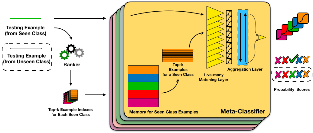
Figure 1. Overview of the L2AC framework (best viewed in colors). Assume the seen class set $S$ has 5 classes and their examples are indicated by 5 different colors. L2AC has two components: a ranker and a meta-classifier. Given a (green) testing example from a seen class, the ranker first retrieves the top-$k$ nearest examples (memory indexes) from each seen class. Then the meta-classifier takes both the test example and the top-$k$ nearest examples for a seen class to produce a probability score for that class. The meta-classifier is applied 5 times (indicated by 5 rounded rectangles) over these 5 seen classes and yields 5 probability scores, where the 3rd (green) class attends the maximum score as the final class (green) prediction. However, if the test example (grey) is from an unseen class (as indicated by the dashed box), none of those probability scores from the seen classes will predict positive, which leads rejection.

2.1. Meta-Classifier

Meta-classifier serves as the core component of the L2AC framework. It is essentially a binary classifier on a given seen class. It takes the top-$k$ nearest examples (to the test example $x_{t}$) of the seen class as the input and determines whether $x_{t}$ belongs to that seen class or not. In this section, we first describe how to represent examples of a seen class. Then we describe how the meta-classifier processes these examples together with the test example into an overall probability score (via a voting mechanism) for deciding whether the test example should belong to any seen class (classification) or not (rejection). Along with that we also describe how a joint decision is made for open-world classification over a set of seen classes. Finally, we describe how to train the meta-classifier via another set of meta-training classes and their examples.

2.1.1. Example Representation and Memory

Representation learning lives at the heart of neural networks. Following the success of using pre-trained weights from large-scale image datasets (such as ImageNet (Russakovsky et al., 2015)) as feature encoders, we assume there is an encoder that captures almost all features for text classification.

Given an example $x$ representing a text document (a sequence of tokens), we obtain its continuous representation (a vector) via an encoder $h=g(x)$, where the encoder $g(\cdot)$ is typically a neural network (e.g., CNN or LSTM). We will detail a simple encoder implementation in Sec. 3.

Further, we save the continuous representations of the examples into the memory of the meta-classifier. So later, the top-$k$ examples can be efficiently retrieved via the index (address) in the memory. The memory is essentially a matrix $E\in\mathbb{R}^{n\times|h|}$, where $n$ is the number of all examples from seen classes and $|h|$ is the size of the hidden dimensions. Note that we will still use $x$ instead of $h$ to refer to an example for brevity. Given the test example $x_{t}$, the meta-classifier first looks up the actual continuous representations $x_{a_{1:k}}$ of the top-$k$ examples for a seen class. Then the meta-classifier computes the similarity score between $x_{t}$ and each $x_{a_{i}}$ ($1\leq i\leq k$) individually via a 1-vs-many matching layer as described next.

2.1.2. 1-vs-many Matching Layer

To compute the overall probability between a test example and a seen class, a 1-vs-many matching layer in the meta-classifier first computes the individual similarity score between the test example and each of the top-$k$ retrieved examples of the seen class. The 1-vs-many matching layer essentially consists of $k$ shared matching networks as indicated by big yellow triangles in Fig. 1. We denote each matching network as $f(\cdot,\cdot)$ and compute similarity scores $r_{1:k}$ for all top-$k$ examples $r_{1:k}=f(x_{t},x_{a_{1:k}})$.

The matching network first transforms the test example $x_{t}$ and $x_{a_{i}}$ from the continuous representation space to a single example in a similarity space. We leverage two similarity functions to obtain the similarity space. The first function is the absolute values of the element-wise subtraction: $f_{\text{abssub}}(x_{t},x_{a_{i}})=|x_{t}-x_{a_{i}}|$. The second one is the element-wise summation: $f_{\text{sum}}(x_{t},x_{a_{i}})=x_{t}+x_{a_{i}}$. Then the final similarity space is the concatenation of these two functions’ results: $f_{\text{sim}}(x_{t},x_{a_{i}})=f_{\text{abssub}}(x_{t},x_{a_{i}})\oplus f_{\text{sum}}(x_{t},x_{a_{i}})$, where $\oplus$ denotes the concatenation operation. We then pass the result to two fully-connected layers (one with Relu activation) and a sigmoid function:

(1) $$r_{i}=f(x_{t},x_{a_{i}})=\sigma\Big{(}W_{2}\cdot\text{Relu}\big{(}W_{1}\cdot f_{\text{sim}}(x_{t},x_{a_{i}})+b_{1}\big{)}+b_{2}\Big{)}.$$

Since there are $k$ nearest examples, we have $k$ similarity scores denoted as $r_{1:k}$. The hyper-parameters are detailed in Sec. 3.

2.1.3. Open-world Learning via Aggregation Layer

After getting the individual similarity scores, an aggregation layer in the meta-classifier merges the $k$ similarity scores into a single probability indicating whether the test example $x_{t}$ belongs to the seen class. By having the aggregation layer, the meta-classifier essentially has a parametric voting mechanism so that it can learn how to vote on multiple nearest examples (rather than a single example) from a seen class to decide the probability. As a result, the meta-classifier can have more reliable predictions, which is studied in Sec. 3.

We adopt a (many-to-one) BiLSTM (Hochreiter and Schmidhuber, 1997; Schuster and Paliwal, 1997) as the aggregation layer. We set the output size of BiLSTM to 2 (1 per direction of LSTM). Then the output of BiLSTM is connected to a fully-connected layer followed by a sigmoid function that outputs the probability. The computation of the meta-classifier for a given test example $x_{t}$ and $x_{a_{1:k}}$ for a seen class $c$ can be summarized as:

(2) $$p(c|x_{t},x_{a_{1:k}})=\sigma\big{(}W\cdot\text{BiLSTM}(r_{1:k})+b\big{)}.$$

Inspired by DOC (Shu et al., 2017), for each class $c\in S$, we evaluate Eq. 2 as:

(3) $$\hat{y}=\left\{\begin{array}[]{c}\textit{reject},\text{ if }\max_{c\in S}p(c|x_{t},x_{a_{1:k}})\leq 0.5;\\ \\ \operatorname*{arg\,max}_{c\in S}p(c|x_{t},x_{a_{1:k}}),\text{ otherwise.}\end{array}\right.$$

If none of existing seen classes $S$ gives a probability above $0.5$, we reject $x_{t}$ as an example from some unseen class. Note that given a large number of classes, eq. 3 can be efficiently implemented in parallel. We leave this to future work. To make L2AC an easily accessible approach, we use $0.5$ as the threshold naturally and do not introduce an extra hyper-parameter that needs to be artificially tuned. Note also that as discussed earlier, the seen class set $S$ and its examples can be dynamically maintained (e.g., one can add to or remove from $S$ any class). So the meta-classifier simply performs open-world classification over the current seen class set $S$.

2.2. Training of Meta-Classifier

Since the meta-classifier is a general classifier that is supposed to work for any class, training the meta-classifier $p_{\theta}(c|x_{t},x_{a_{1:k}|x_{t},c})$ requires examples from another set $M$ of classes called meta-training classes. A large $|M|$ is desirable so that meta-training classes have good coverage of features for seen and unseen classes in testing, which is in similar spirit to few-shot learning (Lake et al., 2011). We also enforce $(S\cup U)\cap M=\varnothing$ in Sec. 3, so that all seen and unseen classes are totally unknown to the meta-classifier.

Next, we formulate the meta-training examples from $M$, which consist of a set of pairs (with positive and negative labels). The first component of a pair is a training document $x_{q}$ from a class in $M$, and the second component is a sequence of top-$k$ nearest examples also from a class in $M$.

We assume every example (document) of a class in $M$ can be a training document $x_{q}$. Assuming $x_{q}$ is from class $c\in M$, a positive training pair is $(x_{q},x_{a_{1:k}|x_{q},c})$, where $x_{a_{1:k}|x_{q},c}$ are top-$k$ examples from class $c$ that are most similar or nearest to $x_{q}$; a negative training pair is $(x_{q},x_{a_{1:k}|x_{q},c^{\prime}})$, where $c^{\prime}\in M$, $c\neq c^{\prime}$ and $x_{a_{1:k}|x_{q},c^{\prime}}$ are top-$k$ examples from class $c^{\prime}$ that are nearest to $x_{q}$. We call $c^{\prime}$ one negative class for $x_{q}$. Since there are many negative classes $c^{\prime}\in M\backslash c$ for $x_{q}$, we keep top-$n$ negative classes for each training example $x_{q}$. That is, each $x_{q}$ has one positive training pair and $n$ negative training pairs. To balance the classes in the training loss, we give a weight ratio $n:1$ for a positive and a negative pair, respectively.

Training the meta-classifier also requires validation classes for model selection (during optimization) and hyper-parameters ($k$ and $n$) tuning (as detailed in Experiments). Since the classes tested by the meta-classifier are unexpected, we further use a set of validation classes $M^{\prime}\cap M=\varnothing$ (also $M^{\prime}\cap(S\cup U)=\varnothing$), to ensure generalization on the seen/unseen classes.

3. Experiments

We want to address the following Research Questions (RQs): RQ1 - what is the performance of the meta-classifier with different settings of top-$k$ examples and $n$ negative classes? RQ2 - How is the performance of L2AC compared with state-of-the-art text classifiers for open-world classification (which all need some forms of re-training).

3.1. Dataset

We leverage the huge amount of product descriptions from the Amazon Datasets (He and McAuley, 2016) and form the OWL task as the following. Amazon.com maintains a tree-structured category system. We consider each path to a leaf node as a class. We removed products belonging to multiple classes to ensure the classes have no overlapping. This gives us 2598 classes, where 1018 classes have more than 400 products per class. We randomly choose 1000 classes from the 1018 classes with 400 randomly selected products per class as the encoder training set; 100 classes with 150 products per class are used as the (classification) test set, including both seen classes $S$ and unseen classes $U$; another 1000 classes with 100 products per class are used as the meta-training set (including both $M$ and $M^{\prime}$). For the 100 classes of the test set, we further hold out 50 examples (products) from each class as test examples. The rest 100 examples are training data for baselines, or seen classes examples to be read by the meta-classifier (which only reads those examples but is not trained on those examples). To train the meta-classifier, we further split the meta-training set as 900 meta-training classes ($M$) and 100 validation classes ($M^{\prime}$).

For all datasets, we use NLTK as the tokenizer, and regard all words that appear more than once as the vocabulary. This gives us 17,526 unique words. We take the maximum length of each document as 120 since the majority of product descriptions are under 100 words.

3.2. Ranker

We use cosine similarity to rank the examples in each seen (or meta-training) class for a given test (or meta-training) example $x_{t}$ (or $x_{q}$). We apply cosine directly on the hidden representations of the encoder as $cosine(h_{*},h_{a_{i}})=\frac{h_{*}\cdot h_{a_{i}}}{|h_{*}|_{2}|h_{a_{i}}|_{2}}$, where $*$ can be either $t$ or $q$, $|\cdot|_{2}$ denotes the $l$-2 norm and $\cdot$ denotes the dot product of two examples.

Training the meta-classifier also requires a ranking of negative classes for a meta-training example $x_{q}$, as discussed in Sec. 2.2. We first compute a class vector for each meta-training class. This class vector is averaged over all encoded representations of examples of that class. Then we rank classes by computing cosine similarity between the class vectors and the meta-training example $x_{q}$. The top-$n$ (defined in the previous section) classes are selected as negative classes for $x_{q}$. We explore different settings of $n$ later.

3.3. Evaluation

Similar to (Shu et al., 2017), we choose 25, 50, and 75 classes from the (classification) test set of 100 classes as the seen classes for three (3) experiments. Note that each class in the test set has 150 examples, where 100 examples are for the training of baseline methods or used as seen class examples for L2AC and 50 examples are for testing both the baselines and L2AC. We evaluate the results on all 100 classes for those three (3) experiments. For example, when there are 25 seen classes, testing examples from the rest 75 unseen classes are taken as from one rejection class $c_{\text{rej}}$, as in (Shu et al., 2017).

Besides using macro F1 as used in (Shu et al., 2017), we also use weighted F1 score overall classes (including seen and the rejection class) as the evaluation metric. Weighted F1 is computed as

(4) $$\sum_{c\in S\cup\{c_{\text{rej}}\}}\frac{N_{c}}{\sum_{c\in S\cup\{c_{\text{rej}}\}}N_{c}}\cdot\text{F1}_{c},$$

where $N_{c}$ is the number of examples for class $c$ and $\text{F1}_{c}$ is the F1 score of that class. We use this metric because macro F1 has a bias on the importance of rejection when the seen class set is small (macro F1 treats the rejection class as equally important as one seen class). For example, when the number of seen classes is small, the rejection class should have a higher weight as a classifier on a small seen set is more likely challenged by examples from unseen classes. Further, to stabilize the results, we train all models with 10 different initializations and average the results.

3.4. Hyper-parameters

For simplicity, we leverage a BiLSTM (Hochreiter and Schmidhuber, 1997; Schuster and Paliwal, 1997) on top of a GloVe (Pennington et al., 2014) embedding (840b.300d) layer as the encoder (other choices are also possible). Similar to feature encoders trained from ImageNet (Russakovsky et al., 2015), we train classification over the encoder training set with 1000 classes and use 5% of the encoding training data as encoder validation data. We apply dropout rates of 0.5 to all layers of the encoder. The classification accuracy of the encoder on validation data is 81.76%. The matching network (the shared network within the 1-vs-many matching layer) has two fully-connected layers, where the size of the hidden dimension is 512 with a dropout rate of 0.5. We set the batch size of meta-training as 256.

To answer RQ1 on two hyper-parameters $k$ (number of nearest examples from each class) and $n$ (number of negative classes), we use the 100 validation classes to determine these two hyper-parameters. We formulate the validation data similar to the testing experiment on 50 seen classes. For each validation class, we select 50 examples for validation. The rest 50 examples from each validation seen class are used to find top-$k$ nearest examples. We perform grid search of averaged weighted F1 over 10 runs for $k\in\{1,3,5,10,15,20\}$ and $n\in\{1,3,5,9\}$, where $k=5$ and $n=9$ reach a reasonably well weighted F1 (87.60%). Further increasing $n$ gives limited improvements (e.g., 87.69% for $n=14$ and 87.68% for $n=19$, when $k=5$). But a large $n$ significantly increases the number of training examples (e.g., $n=14$ ended with more than 1 million meta-training examples) and thus training time. So we decide to select $k=5$ and $n=9$ for all ablation studies below. Note the validation classes are also used to compute (formulated in a way similar to the meta-training classes) the validation loss for selecting the best model during Adam (Kingma and Ba, 2014) optimization.

3.5. Compared Methods

Methods	$|S|=25$ (WF1)	$|S|=25$ (MF1)	$|S|=50$ (WF1)	$|S|=50$ (MF1)	$|S|=75$ (WF1)	$|S|=75$ (MF1)
DOC-CNN	53.25(1.0)	55.04(0.39)	70.57(0.46)	76.91(0.27)	81.16(0.47)	86.96(0.2)
DOC-LSTM	57.87(1.26)	57.6(1.18)	69.49(1.58)	75.68(0.78)	77.74(0.48)	84.48(0.33)
DOC-Enc	82.92(0.37)	75.09(0.33)	82.53(0.25)	84.34(0.23)	83.84(0.36)	88.33(0.19)
DOC-CNN-Gaus	85.72(0.43)	76.79(0.41)	83.33(0.31)	83.75(0.26)	84.21(0.12)	87.86(0.21)
DOC-LSTM-Gaus	80.31(1.73)	70.49(1.55)	77.49(0.74)	79.45(0.59)	80.65(0.51)	85.46(0.25)
DOC-Enc-Gaus	88.54(0.22)	80.77(0.22)	84.75(0.21)	85.26(0.2)	83.85(0.37)	87.92(0.22)
L2AC-$n$9-NoVote	91.1(0.17)	82.51(0.39)	84.91(0.16)	83.71(0.29)	81.41(0.54)	85.03(0.62)
L2AC-$n$9-Vote3	91.54(0.55)	82.42(1.29)	84.57(0.61)	82.7(0.95)	80.18(1.03)	83.52(1.14)
L2AC-$k$5-$n$9-AbsSub	92.37(0.28)	84.8(0.54)	85.61(0.36)	84.54(0.42)	83.18(0.38)	86.38(0.36)
L2AC-$k$5-$n$9-Sum	83.95(0.52)	70.85(0.91)	76.09(0.36)	75.25(0.42)	74.12(0.51)	78.75(0.57)
L2AC-$k$5-$n$9	93.07(0.33)	86.48(0.54)	86.5(0.46)	85.99(0.33)	84.68(0.27)	88.05(0.18)
L2AC-$k$5-$n$14	93.19(0.19)	86.91(0.33)	86.63(0.28)	86.42(0.2)	85.32(0.35)	88.72(0.23)
L2AC-$k$5-$n$19	93.15(0.24)	86.9(0.45)	86.62(0.49)	86.48(0.43)	85.36(0.66)	88.79(0.52)

Table 1. Weighted F1 (WF1) and macro F1 (MF1) scores on a test set with 100 classes with 3 settings: 25, 50, and 75 seen classes. The set of seen classes are incrementally expanded from 25 to 75 classes (or gradually shrunk from 75 to 25 classes). The results are the averages over 10 runs with standard deviations in parenthesis.

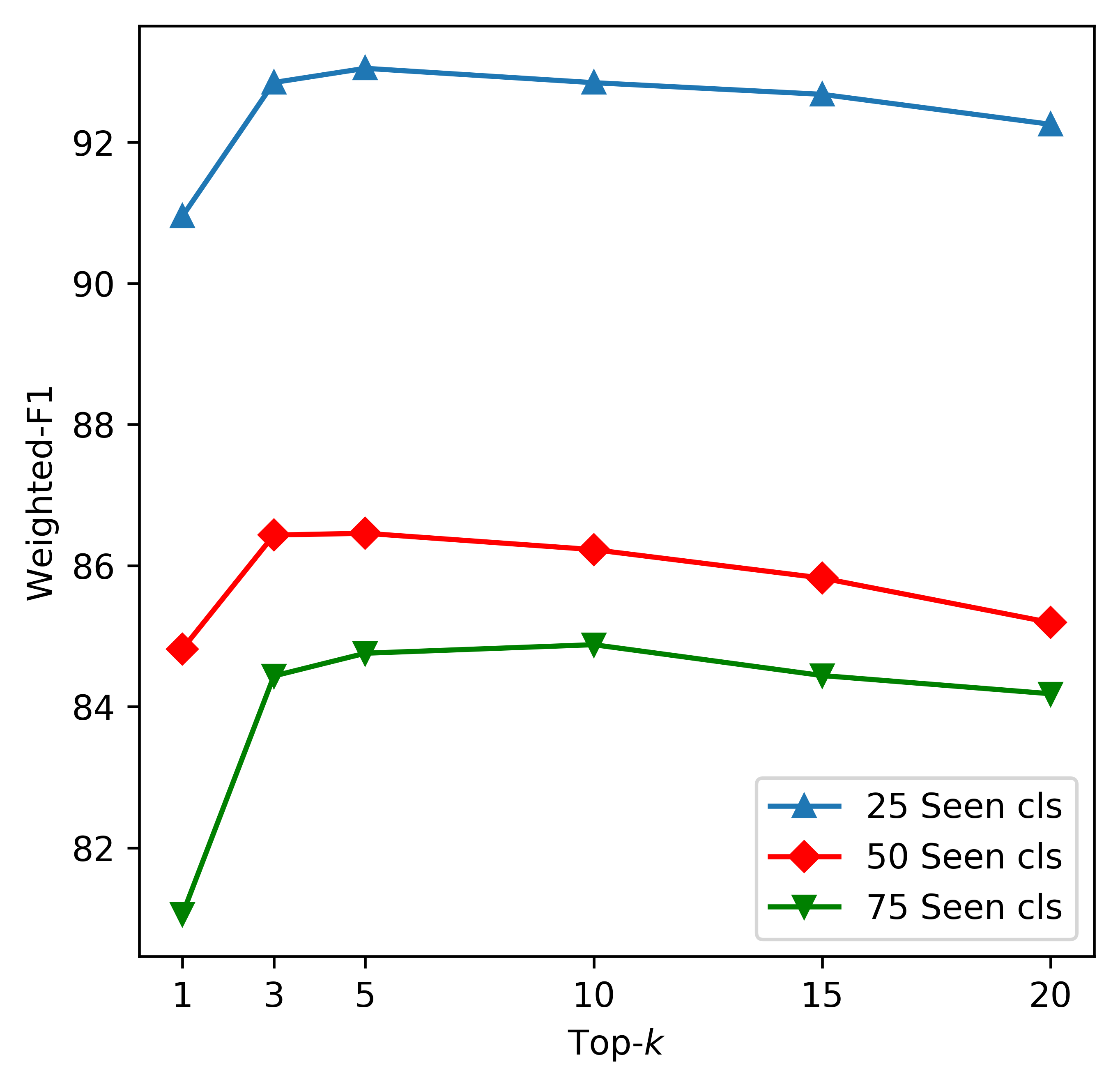
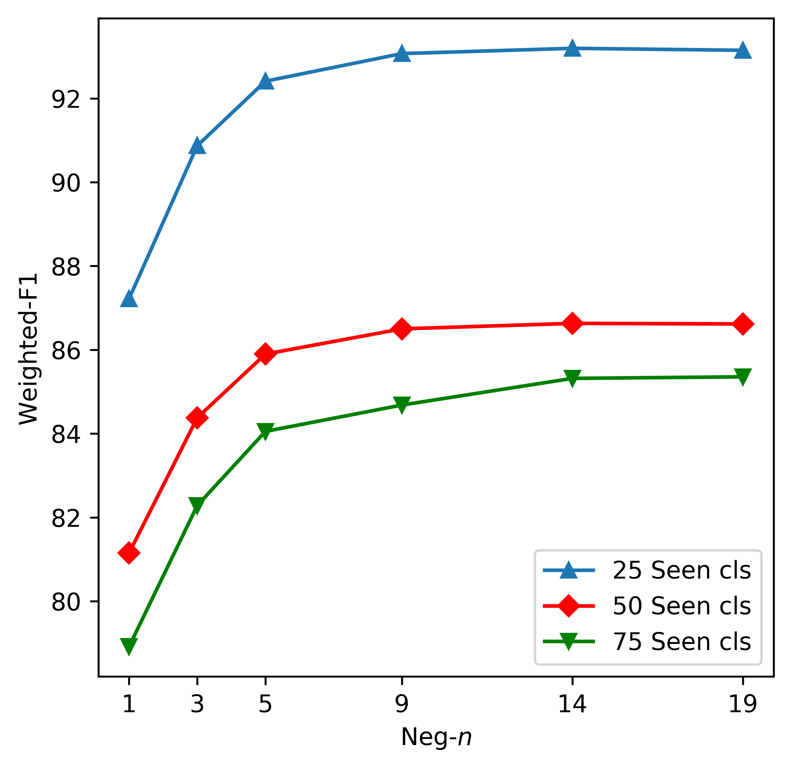
Figure 2. Weighted F1 scores for different $k$’s ($n=9$) and different $n$’s ($k=5$).

To the best of our knowledge, DOC (Shu et al., 2017) is the only state-of-the-art baseline for open-world learning (with rejection) for text classification. It has been shown in (Shu et al., 2017) that DOC significantly outperforms the methods CL-cbsSVM and cbsSVM in (Fei et al., 2016) and OpenMax in (Bendale and Boult, 2016). OpenMax is a state-of-the-art method for image classification with rejection capability.

To answer RQ2, we use DOC and its variants to show that the proposed method has comparable performance with the best open-world learning method with re-training. Note that DOC cannot incrementally add new classes. So we re-train DOC over different sets of seen classes from scratch every time new classes are added to that set. It is thus actually unfair to compare our method with DOC because DOC is trained on the actual training examples of all classes. However, our method still performs better in general. We used the original code of DOC and created six (6) variants of it.

DOC-CNN: CNN implementation as in the original DOC paper without Gaussian fitting (using 0.5 as the threshold for rejection). It operates directly on a sequence of tokens.
DOC-LSTM: a variant of DOC-CNN, where we replace CNN with BiLSTM to encode the input sequence for fair comparison. BiLSTM is trainable and the input is still a sequence of tokens.
DOC-Enc: this is adapted from DOC-CNN, where we remove the feature learning part of DOC-CNN and feed the hidden representation from our encoder directly to the fully-connected layers of DOC for a fair comparison with L2AC.
DOC-*-Gaus: applying Gaussian fitting proposed in (Shu et al., 2017) on the above three baselines, we have 3 more DOC baselines. Note that these 3 baselines have exactly the same models as above respectively. They only differ in the thresholds used for rejection. Gaussian fitting in (Shu et al., 2017) is used to set a good threshold for rejection. We use these baselines to show that the Gaussian fitted threshold improves the rejection performance of DOC significantly but may lower the performance of seen class classification. The original DOC is DOC-CNN-Gaus here.

The following baselines are variants of L2AC.
L2AC-$n$9-NoVote: this is a variant of the proposed L2AC that only takes one most similar example (from each class), i.e., $k=1$, with one positive class paired with $n=9$ negative classes in meta-training ($n=9$ has the best performance as indicated in answering RQ1 above). We use this baseline to show that the performance of taking only one sample may not be good enough. This baseline clearly does not have/need the aggregation layer and only has a single matching network in the 1-vs-many layer.
L2AC-$n$9-Vote3: this baseline uses exactly the same model as L2AC-$n$9-NoVote. But during evaluation, we allow a non-parametric voting process (like $k$NN) for prediction. We report the results of voting over top-3 examples per seen class as it has the best result (ranging from 3 to 10). If the average of the top-3 similar examples in a seen class has example scores with more than $0.5$, L2AC believes the testing example belongs to that class. We use this baseline to show that the aggregation layer is effective in learning to vote and L2AC can use more similar examples and get better performance.
L2AC-$k$5-$n$9-AbsSub/Sum: To show that using two similarity functions ($f_{\text{abssub}}(\cdot,\cdot)$ and $f_{\text{sum}}(\cdot,\cdot)$ ) gives better results, we further perform ablation study by using only one of those similarity functions at a time, which gives us two baselines.
L2AC-$k$5-$n$9/14/19: this baseline has the best $k=5$ and $n=9$ on the validation classes, as indicated in the previous subsection. Interestingly, further increasing $k$ may reduce the performance as L2AC may focus on not-so-similar examples. We also report results on $n=14$ or $19$ to show that the results do not get much better.

3.6. Results Analysis

From Table 1, we can see that L2AC outperforms DOC, especially when the number of seen classes is small. First, from Fig. 2 we can see that $k=5$ and $n=9$ gets reasonably good results. Increasing $k$ may harm the performance as taking in more examples from a class may let L2AC focus on not-so-similar examples, which is bad for classification. More negative classes give L2AC better performance in general but further increasing $n$ beyond 9 has little impact.

Next, we can see that as we incrementally add more classes, L2AC gradually drops its performance (which is reasonable due to more classes) but it still yields better performance than DOC. Considering that L2AC needs no training with additional classes, while DOC needs full training from scratch, L2AC represents a major advance. Note that testing on 25 seen classes is more about testing a model’s rejection capability while testing on 75 seen classes is more about the classification performance of seen class examples. From Table 1, we notice that L2AC can effectively leverage multiple nearest examples and negative classes. In contrast, the non-parametric voting of L2AC-$n$9-Vote3 over top-3 examples may not improve the performance but introduce higher variances. Our best $k=5$ indicates that the meta-classifier can dynamically leverage multiple nearest examples instead of solely relying on a single example. As an ablation study on the choices of similarity functions, running L2AC on a single similarity function gives poorer results as indicated by either L2AC-$k$5-$n$9-AbsSub or L2AC-$k$5-$n$9-Sum.

DOC without encoder (DOC-CNN or DOC-LSTM) performs poorly when the number of seen classes is small. Without Gaussian fitting, DOC’s (DOC-CNN, DOC-LSTM or DOC-Enc) performance increases as more classes are added as seen classes. This is reasonable as DOC is more challenged by fewer seen training classes and more unseen classes during testing. As such, Gaussian fitting (DOC-*-Gaus) alleviates the weakness of DOC on a small number of seen training classes.

4. Related Work

Open-world learning has been studied in text mining and computer vision (where it is called open-set recognition) (Bendale and Boult, 2015; Chen and Liu, 2018; Fei et al., 2016). Most existing approaches focus on building a classifier that can predict examples from unseen classes into a (hidden) rejection class. These solutions are built on top of closed-world classification models (Bendale and Boult, 2015, 2016; Shu et al., 2017). Since a closed-world classifier cannot detect/reject examples from unseen classes (they will be classified into some seen classes), some thresholds are used so that these closed-world models can also be used to do rejection. However, as discussed earlier, when incrementally learning new classes, they also need some form of re-training, either full re-training from scratch (Bendale and Boult, 2016; Shu et al., 2017) or partial re-training in an incremental manner (Bendale and Boult, 2015; Fei et al., 2016).

Our work is also related to class incremental learning (Rebuffi et al., 2017; Rusu et al., 2016; Lee et al., 2017), where new classes can be added dynamically to the classifier. For example, iCaRL (Rebuffi et al., 2017) maintains some exemplary data for each class and incrementally tunes the classifier to support more new classes. However, they also require training when each new class is added.

Our work is clearly related to meta-learning (or learning to learn) (Thrun and Pratt, 2012), which turns the machine learning tasks themselves as training data to train a meta-model and has been successfully applied to many machine learning tasks lately, such as (Andrychowicz et al., 2016; Fernando et al., 2017; Finn et al., 2017, 2018; Fan et al., 2018). Our proposed framework focuses on learning the similarity between an example and an arbitrary class and we are not aware of any open-world learning work based on meta-learning.

The proposed framework is also related to zero-shot learning (Lampert et al., 2009; Palatucci et al., 2009; Socher et al., 2013) (in that we do not require training but need to read training examples), $k$-nearest neighbors ($k$NN) (with additional rejection capability, metric learning (Xing et al., 2003) and learning to vote), and Siamese networks (Bromley et al., 1994; Koch et al., 2015; Vinyals et al., 2016) (regarding processing a pair of examples). However, all those techniques work in closed-worlds with no rejection capability.

Product classification has been studied in (Shen et al., 2011, 2012; Chen and Warren, 2013; Gupta et al., 2016; Cevahir and Murakami, 2016; Kozareva, 2015), mostly in a multi-level (or hierarchical) setting. However, given the dynamic taxonomy in nature, product classification has not been studied as an open-world learning problem.

5. Conclusions

In this paper, we proposed a meta-learning framework called L2AC for open-world learning. L2AC has been applied to product classification. Compared to traditional closed-world classifiers, our meta-classifier can incrementally accept new classes by simply adding new class examples without re-training. Compared to other open-world learning methods, the rejection capability of L2AC is trained rather than realized using some empirically set thresholds. Our experiments showed superior performances to strong baselines.

References

- (1)
- Andrychowicz et al. (2016) Marcin Andrychowicz, Misha Denil, Sergio Gomez, Matthew W Hoffman, David Pfau, Tom Schaul, Brendan Shillingford, and Nando De Freitas. 2016. Learning to learn by gradient descent by gradient descent. In NIPS. 3981–3989.
- Bendale and Boult (2015) Abhijit Bendale and Terrance Boult. 2015. Towards open world recognition. In Proceedings of the IEEE Conference on Computer Vision and Pattern Recognition. 1893–1902.
- Bendale and Boult (2016) Abhijit Bendale and Terrance E Boult. 2016. Towards open set deep networks. In Proceedings of the IEEE conference on computer vision and pattern recognition. 1563–1572.
- Bromley et al. (1994) Jane Bromley, Isabelle Guyon, Yann LeCun, Eduard Säckinger, and Roopak Shah. 1994. Signature verification using a” siamese” time delay neural network. In Advances in Neural Information Processing Systems. 737–744.
- Cevahir and Murakami (2016) Ali Cevahir and Koji Murakami. 2016. Large-scale Multi-class and Hierarchical Product Categorization for an E-commerce Giant. In Proceedings of COLING 2016, the 26th International Conference on Computational Linguistics: Technical Papers. 525–535.
- Chen and Warren (2013) Jianfu Chen and David Warren. 2013. Cost-sensitive learning for large-scale hierarchical classification. In Proceedings of the 22nd ACM international conference on Conference on information & knowledge management. ACM, 1351–1360.
- Chen and Liu (2018) Zhiyuan Chen and Bing Liu. 2018. Lifelong machine learning. Morgan & Claypool Publishers.
- Fan et al. (2018) Yang Fan, Fei Tian, Tao Qin, Xiang-Yang Li, and Tie-Yan Liu. 2018. Learning to Teach. arXiv preprint arXiv:1805.03643 (2018).
- Fei et al. (2016) Geli Fei, Shuai Wang, and Bing Liu. 2016. Learning cumulatively to become more knowledgeable. In Proceedings of the 22nd ACM SIGKDD International Conference on Knowledge Discovery and Data Mining. ACM, 1565–1574.
- Fernando et al. (2017) Chrisantha Fernando, Dylan Banarse, Charles Blundell, Yori Zwols, David Ha, Andrei A Rusu, Alexander Pritzel, and Daan Wierstra. 2017. Pathnet: Evolution channels gradient descent in super neural networks. arXiv preprint arXiv:1701.08734 (2017).
- Finn et al. (2017) Chelsea Finn, Pieter Abbeel, and Sergey Levine. 2017. Model-Agnostic Meta-Learning for Fast Adaptation of Deep Networks. In International Conference on Machine Learning. 1126–1135.
- Finn et al. (2018) Chelsea Finn, Kelvin Xu, and Sergey Levine. 2018. Probabilistic Model-Agnostic Meta-Learning. arXiv preprint arXiv:1806.02817 (2018).
- Gupta et al. (2016) Vivek Gupta, Harish Karnick, Ashendra Bansal, and Pradhuman Jhala. 2016. Product Classification in E-Commerce using Distributional Semantics. In Proceedings of COLING 2016, the 26th International Conference on Computational Linguistics: Technical Papers. 536–546.
- He and McAuley (2016) Ruining He and Julian McAuley. 2016. Ups and downs: Modeling the visual evolution of fashion trends with one-class collaborative filtering. In proceedings of the 25th international conference on world wide web. International World Wide Web Conferences Steering Committee, 507–517.
- Hochreiter and Schmidhuber (1997) Sepp Hochreiter and Jürgen Schmidhuber. 1997. Long short-term memory. Neural computation 9, 8 (1997), 1735–1780.
- Kim et al. (2018) Young-Bum Kim, Dongchan Kim, Anjishnu Kumar, and Ruhi Sarikaya. 2018. Efficient Large-Scale Domain Classification with Personalized Attention. arXiv preprint arXiv:1804.08065 (2018).
- Kingma and Ba (2014) Diederik P Kingma and Jimmy Ba. 2014. Adam: A method for stochastic optimization. arXiv preprint arXiv:1412.6980 (2014).
- Koch et al. (2015) Gregory Koch, Richard Zemel, and Ruslan Salakhutdinov. 2015. Siamese neural networks for one-shot image recognition. In ICML Deep Learning Workshop, Vol. 2.
- Kozareva (2015) Zornitsa Kozareva. 2015. Everyone likes shopping! multi-class product categorization for e-commerce. In Proceedings of the 2015 Conference of the North American Chapter of the Association for Computational Linguistics: Human Language Technologies. 1329–1333.
- Kumar et al. (2017) Anjishnu Kumar, Pavankumar Reddy Muddireddy, Markus Dreyer, and Björn Hoffmeister. 2017. Zero-Shot Learning Across Heterogeneous Overlapping Domains.. In INTERSPEECH. 2914–2918.
- Lake et al. (2011) Brenden Lake, Ruslan Salakhutdinov, Jason Gross, and Joshua Tenenbaum. 2011. One shot learning of simple visual concepts. In Proceedings of the Annual Meeting of the Cognitive Science Society, Vol. 33.
- Lampert et al. (2009) Christoph H Lampert, Hannes Nickisch, and Stefan Harmeling. 2009. Learning to detect unseen object classes by between-class attribute transfer. In Computer Vision and Pattern Recognition, 2009. CVPR 2009. IEEE Conference on. IEEE, 951–958.
- Lee et al. (2017) Jeongtae Lee, Jaehong Yun, Sungju Hwang, and Eunho Yang. 2017. Lifelong Learning with Dynamically Expandable Networks. arXiv preprint arXiv:1708.01547 (2017).
- Palatucci et al. (2009) Mark Palatucci, Dean Pomerleau, Geoffrey E Hinton, and Tom M Mitchell. 2009. Zero-shot learning with semantic output codes. In NIPS. 1410–1418.
- Pennington et al. (2014) Jeffrey Pennington, Richard Socher, and Christopher Manning. 2014. Glove: Global vectors for word representation. In Proceedings of the 2014 conference on empirical methods in natural language processing (EMNLP). 1532–1543.
- Rebuffi et al. (2017) Sylvestre-Alvise Rebuffi, Alexander Kolesnikov, Georg Sperl, and Christoph H Lampert. 2017. iCaRL: Incremental Classifier and Representation Learning. In Computer Vision and Pattern Recognition (CVPR), 2017 IEEE Conference on. IEEE, 5533–5542.
- Russakovsky et al. (2015) Olga Russakovsky, Jia Deng, Hao Su, Jonathan Krause, Sanjeev Satheesh, Sean Ma, Zhiheng Huang, Andrej Karpathy, Aditya Khosla, Michael Bernstein, et al. 2015. Imagenet large scale visual recognition challenge. International Journal of Computer Vision 115, 3 (2015), 211–252.
- Rusu et al. (2016) Andrei A Rusu, Neil C Rabinowitz, Guillaume Desjardins, Hubert Soyer, James Kirkpatrick, Koray Kavukcuoglu, Razvan Pascanu, and Raia Hadsell. 2016. Progressive neural networks. arXiv preprint arXiv:1606.04671 (2016).
- Schuster and Paliwal (1997) Mike Schuster and Kuldip K Paliwal. 1997. Bidirectional recurrent neural networks. IEEE Transactions on Signal Processing 45, 11 (1997), 2673–2681.
- Shen et al. (2012) Dan Shen, Jean-David Ruvini, and Badrul Sarwar. 2012. Large-scale item categorization for e-commerce. In Proceedings of the 21st ACM international conference on Information and knowledge management. ACM, 595–604.
- Shen et al. (2011) Dan Shen, Jean David Ruvini, Manas Somaiya, and Neel Sundaresan. 2011. Item categorization in the e-commerce domain. In Proceedings of the 20th ACM international conference on Information and knowledge management. ACM, 1921–1924.
- Shu et al. (2017) Lei Shu, Hu Xu, and Bing Liu. 2017. DOC: Deep Open Classification of Text Documents. In Proceedings of the 2017 Conference on Empirical Methods in Natural Language Processing. Association for Computational Linguistics, Copenhagen, Denmark, 2911–2916. https://www.aclweb.org/anthology/D17-1314
- Socher et al. (2013) Richard Socher, Milind Ganjoo, Christopher D Manning, and Andrew Ng. 2013. Zero-shot learning through cross-modal transfer. In NIPS. 935–943.
- Thrun and Pratt (2012) Sebastian Thrun and Lorien Pratt. 2012. Learning to learn. Springer.
- Vinyals et al. (2016) Oriol Vinyals, Charles Blundell, Tim Lillicrap, Daan Wierstra, et al. 2016. Matching networks for one shot learning. In Advances in Neural Information Processing Systems. 3630–3638.
- Xing et al. (2003) Eric P Xing, Michael I Jordan, Stuart J Russell, and Andrew Y Ng. 2003. Distance metric learning with application to clustering with side-information. In Advances in neural information processing systems. 521–528.