An inexact PAM method for computing Wasserstein barycenter with unknown supports

Abstract

Wasserstein barycenter is the centroid of a collection of discrete probability distributions which minimizes the average of the $\ell_{2}$-Wasserstein distance. This paper focuses on the computation of Wasserstein barycenters under the case where the support points are free, which is known to be a severe bottleneck in the D2-clustering due to the large-scale and nonconvexity. We develop an inexact proximal alternating minimization (iPAM) method for computing an approximate Wasserstein barycenter, and provide its global convergence analysis. This method can achieve a good accuracy with a reduced computational cost when the unknown support points of the barycenter have low cardinality. Numerical comparisons with the 3-block B-ADMM in YeWWL17 and an alternating minimization method involving the LP subproblems on synthetic and real data show that the proposed iPAM can yield comparable even a little better objective values in less CPU time, and hence the computed barycenter will render a better role in the D2-clustering.

1 Introduction

In machine learning, many complex instances such as images, sequences, and documents can be described in terms of discrete probability distributions. For example, the bag of “words” data model used in multimedia retrieval and document analysis is a discrete distribution, while the widely used normalized histogram which contains the fixed supports and associated weights is also a special case of discrete distributions. In this paper, we focus on the computation of the centroid of discrete probability distributions under the Wasserstein distance (also known as the Mallows distance Mallows72 or the earth mover’s distance Rubner00 ), which is called the Wasserstein barycenter.

Wasserstein barycenters are often used to cluster the discrete probability distributions in D2-clustering, which minimizes the total within-cluster variation under the Wasserstein distance similarly as Lloyd’s K-means for vectors under the Euclidean distance. This clustering problem was originally explored by Li and Wang Li08 who coined the phrase D2-clustering. The motivations for using the Wasserstein distance in practice are strongly argued by some researchers in the literature (see, e.g., Li08 ; Cui13 ; Cui14 ; Pele09 ), and its theoretical significance is well supported in the optimal transport literature Villani08 . In the D2-clustering framework, the Wasserstein barycenter is required for the case of unknown supports with a pre-given cardinality. To compute it, one faces a large-scale nonconvex optimization problem in which a coupled nonconvex objective function is minimized over a polyhedral set. Due to the advantages of Wasserstein distance, D2-clustering holds much promise, but the high computational cost of barycenter has limited its applications.

To scale up the computation of Wasserstein barycenter in the D2-clustering, a divide-and-conquer approach has been proposed in Zhang15 , but the method is ad-hoc and lack of convergence guarantee. When an alternating minimization strategy is used, the computation of Wasserstein barycenter is decomposed into a quadratic program with a closed form solution and a linear program (LP) with a super-linear time-complexity on the number of samples $N$. The latter brings a big challenge for the computation of a barycenter because the number of variables in the LP grows quickly with the number of support points, and the classical LP solvers such as the simplex method and the interior point method are not scalable (see Figure 2, 4 and 6). To overcome this challenge, Ye and Li YeLi14 applied the classical alternating direction method of multipliers (ADMM) for solving this LP, Wang and Banerjee Wang14 generalized the classical ADMM to the Bregman ADMM (B-ADMM) by replacing the quadratic distance with a general Bregman distance so as to exploit the structure of the LP, and Yang et al. Yang18 recently proposed a very efficient dual solver for the LP by adopting a symmetric Gauss-Seidel based ADMM (sGS-ADMM). However, they neither studied the performance of an alternating minimization method with such a subroutine for computing barycenter nor provided the global convergence analysis for the outer alternating minimization method. Recently, Ye et al. YeWWL17 proposed a 3-block B-ADMM for computing a Wasserstein barycenter directly. Although this method has demonstrated a computational efficiency for large-scale data, it is still unclear whether it is globally convergent or not. In fact, for convex programs, it has been shown in Chen16 that the direct extension of the classical ADMM to the three-block case can be divergent.

The main contribution of this work is to develop a globally convergent and efficient inexact proximal alternating minimization (iPAM) method for computing an approximate Wasserstein barycenter when the support points are unknown. Since a proximal alternating minimization strategy is used, each iteration involves two strongly convex quadratic programs (QPs). One of them has a closed form solution, and the other has a polyhedral constraint set and may be good-conditioned by controlling the proximal parameter elaborately. The strongly convex QPs have much better stability than those LPs appearing in YeLi14 ; Wang14 , which means that their solutions are much easier to achieve. In Section 5.1, we propose a tailored linearized ADMM for solving the strongly convex QP by exploiting the special structure of the feasible set. Different from the sGS-ADMM proposed in Yang18 , the linearized ADMM is a primal solver for a 2-block strongly convex QP instead of a dual solver for the 3-block LP. We notice that the B-ADMM in Wang14 also belongs to this line since at each iteration it transforms the LP into two simple strongly convex Kullback-Leibler minimization problems to solve. Compared with the B-ADMM, our linearized ADMM not only has a global convergence FPST13 but also admits the well-established linear rate of convergence HanSZ17 and weighted iteration complexity ShenPan16 . Numerical comparisons with the 3-block B-ADMM in YeWWL17 and an alternating minimization method involving the LP subproblems (ALMLP for short) on synthetic and real data indicate that the proposed iPAM yields comparable even a little better objective values within less computing time, and hence the computed approximate barycenter will render a better role in the D2-clustering.

For a nonconvex and nonsmooth optimization problem, without additional conditions imposed on the problem, the convergence result of an alternating minimization method and more general block coordinate descent methods (see, e.g., Tseng01 ; Tseng09 ; Razaviyayn13 ; Hong16 ) is typically limited to the objective value convergence (to a possibly non-minimal value) or the convergence of a certain subsequence of iterates to a critical point. Motivated by the recent excellent works Attouch10 ; Attouch13 ; Bolte14 , we achieve the global convergence of our iPAM method for computing a Wasserstein barycenter by using the Kurdyka-Lojasiewicz (KL) property of the extended objective function. It is worthwhile to point out that under the KL assumption Xu and Yin Xu17 also developed a globally convergent algorithm based on block coordinate update for a class of nonconvex and nonsmooth optimization problems.

The rest of this paper is organized as follows. Section 2 presents the notation and preliminary knowledge that will be used in this paper. In Section 3, we introduce the optimization model for computing a Wasserstein barycenter when its support points are unknown and propose an inexact PAM method for solving it. Section 4 focuses on the convergence analysis of the iPAM method. In Section 5, we provide the implementation details of the iPAM and compare its performance with that of the B-ADMM YeWWL17 and ALMLP on synthetic and real data.

2 Notation and preliminaries

Throughout this paper, $\mathbb{R}^{m\times n}$ represents the vector space consisting of all $m\times n$ real matrices, equipped with the trace inner product $\langle\cdot,\cdot\rangle$ and its induced Frobenius norm $\|\cdot\|_{F}$, i.e., $\langle X,Y\rangle={\rm tr}(X^{\mathbb{T}}Y)$ for $X,Y\in\mathbb{R}^{m\times n}$, and $\mathbb{R}_{+}^{m\times n}$ denotes the polyhedral cone consisting of all $m\times n$ nonnegative real matrices. For a given vector $x\in\mathbb{R}^{n}$, $\|x\|$ means the Euclidean-norm in $\mathbb{R}^{n}$. For a given set $S$, $\delta_{S}$ denotes the indicator function on $S$, i.e., $\delta_{S}(u)=0$ if $u\in S$, otherwise $\delta_{S}(u)=+\infty$; when $S$ is convex, $\mathcal{N}_{S}(x)$ denotes the normal cone of $S$ at $x$ in the sense of convex analysis Roc70 . The notation $e_{p}$ denotes a column vector of all ones whose dimension is $p$.

In the rest of this section, the notation $\mathbb{X}$ denotes a finite dimensional vector space equipped with the inner product $\langle\cdot,\cdot\rangle$ and its induced norm $\|\cdot\|$. First of all, we recall from (RW98, , Chapter 8) the notion of generalized subdifferentials for an extended real-valued function.

2.1 Generalized subdifferential and critical point

Definition 1

Consider a function $h\!:\mathbb{X}\to(-\infty,+\infty]$ and a point $\overline{x}$ with $h(\overline{x})$ finite. The regular subdifferential of $h$ at $x$, denoted by $\widehat{\partial}h(x)$, is defined as

$$\widehat{\partial}h(x):=\bigg{\{}v\in\mathbb{R}^{p}\ \big{|}\ \liminf_{x^{\prime}\to x\atop x^{\prime}\neq x}\frac{h(x^{\prime})-h(x)-\langle v,x^{\prime}-x\rangle}{\|x^{\prime}-x\|}\geq 0\bigg{\}};$$

and the (limiting) subdifferential of $h$ at $x$, denoted by $\partial h(x)$, is defined as

$$\partial h(x):=\Big{\{}v\in\mathbb{R}^{p}\ |\ \exists\,x^{k}\xrightarrow[h]{}x\ {\rm and}\ v^{k}\in\widehat{\partial}h(x^{k})\to v\ {\rm as}\ k\to\infty\Big{\}}.$$

Remark 1

(a) Notice that $\widehat{\partial}h(\overline{x})\subseteq\partial h(\overline{x})$, and the former is a closed convex set, but the latter is generally not convex. When $h$ is convex, $\partial h(\overline{x})=\widehat{\partial}h(\overline{x})$, which also coincides with the subdifferential of $h$ at $\overline{x}$ in the sense of convex analysis Roc70 .

(b) Let $\{(x^{k},\xi^{k})\}$ be a sequence in the graph of the set-valued mapping $\partial h\!:\mathbb{X}\rightrightarrows\mathbb{X}$, which converges to $(\overline{x},\overline{\xi})$. If $h(x^{k})\to h(\overline{x})$ as $k\to\infty$, then $(\overline{x},\overline{\xi})\in{\rm gph}\partial h$.

(c) By (RW98, , Theorem 10.1), a necessary condition for $\overline{x}\in\mathbb{X}$ to be a local minimizer of $h$ is $0\in\widehat{\partial}h(\overline{x})\subseteq\partial h(\overline{x})$. A point $x^{*}$ satisfying $0\in\partial h(x^{*})$ (respectively, $0\in\widehat{\partial}h(x^{*})$) is called a critical (respectively, regular critical) point of $h$. The critical point set of $h$ is denoted by ${\rm crit}\,h$.

For an optimization problem with a nonconvex objective function but a closed convex feasible set, it is common to consider its directional stationary point, which is defined as follows.

Definition 2

Let $h\!:\mathbb{X}\to\mathbb{R}$ be a directionally differentiable function, and $S\subseteq\mathbb{X}$ be a closed convex set. Consider a point $\overline{x}\in S$. If for every $x\in S$, $h^{\prime}(\overline{x};x-\overline{x})\geq 0,$ then $\overline{x}$ is called a directional stationary point of the minimization problem $\min_{x\in S}h(x)$.

The following lemma states that for the problem in Definition 2, when $h$ is locally Lipschitz relative to $S$ and regular, its directional stationary points are same as the critical point of $h+\delta_{S}$.

Lemma 1

Consider the minimization problem $\min_{x\in S}h(x)$ where $S\subseteq\mathbb{X}$ is a closed convex set. Suppose that $h\!:\mathbb{X}\to\mathbb{R}$ is directionally differentiable and locally Lipschitz at $\widehat{x}\in S$. If $\widehat{x}$ is a directional stationary point of this problem, then $0\in\partial h(\widehat{x})+\mathcal{N}_{S}(\widehat{x})$. If in addition $\partial h(\widehat{x})=\widehat{\partial}h(\widehat{x})$, then every critical point of $h+\delta_{S}$ is a directional stationary point of this problem.

Proof

Write $f(x):=h(x)+\delta_{S}(x)$ for $x\in\mathbb{X}$. From the definition of subderivative and the directional differentiability of $h$, it is not hard to obtain that

$$df(\widehat{x})(w)=h^{\prime}(\widehat{x};w)+\delta_{\mathcal{T}_{S}(\widehat{x})}(w)\quad\forall w\in\mathbb{X}.$$

Since $h^{\prime}(\widehat{x};x-\widehat{x})\geq 0$ for all $x\in S$, from the definition of radial cone, it follows that $h^{\prime}(\widehat{x};w)\geq 0$ for all $w\in\mathcal{R}_{S}(\widehat{x})$. Notice that $\mathcal{T}_{S}(\widehat{x})={\rm cl}[\mathcal{R}_{S}(\widehat{x})]$. From the globally Lipschitz continuity of $h^{\prime}(\widehat{x};\cdot)$, we have $h^{\prime}(\widehat{x};w)\geq 0$ for all $w\in\mathcal{T}_{S}(\widehat{x})$. Together with the last equation, it follows that

$$df(\widehat{x})(w)\geq 0\quad{\rm for\ all}\ w\in\mathbb{X}.$$

Now pick any $(u,\alpha)\in\mathcal{T}_{{\rm epi}f}(\widehat{x},f(\widehat{x}))={\rm epi}\,df(\widehat{x})$ where the equality is due to (RW98, , Theorem 8.2). Then, $\langle(0,-1),(u,\alpha)\rangle=-\alpha\leq-df(\widehat{x})(u)\leq 0,$ which implies that

$$(0,-1)\in[\mathcal{T}_{{\rm epi}f}(\widehat{x},f(\widehat{x}))]^{\circ}=\widehat{\mathcal{N}}_{{\rm epi}f}(\widehat{x},f(\widehat{x}))\subseteq\mathcal{N}_{{\rm epi}f}(\widehat{x},f(\widehat{x})).$$

By (RW98, , Theorem 8.9), it follows that $0\in\partial f(\widehat{x})\subseteq\partial h(\widehat{x})+\mathcal{N}_{S}(\widehat{x})$.

Now suppose that $\partial h(\widehat{x})=\widehat{\partial}h(\widehat{x})$. From $0\in\partial h(\widehat{x})+\mathcal{N}_{S}(\widehat{x})$, we have $0\in\widehat{\partial}h(\widehat{x})+\mathcal{N}_{S}(\widehat{x})$. Then, there exists $s\in\mathcal{N}_{S}(\widehat{x})$ such that $-s\in\widehat{\partial}h(\widehat{x})$. By (RW98, , Exercise 8.4), for any $x\in S$,

$$dh(\widehat{x})(x-\widehat{x})\geq\langle-s,x-\widehat{x}\rangle\geq 0.$$

Notice that $dh(\widehat{x})(x-\widehat{x})=h^{\prime}(\widehat{x};x-\widehat{x})$. So, $h^{\prime}(\widehat{x};x-\widehat{x})\geq 0$ for all $x\in S$. ∎

2.2 Kurdyka-Lojasiewicz property

Definition 3

Let $h\!:\mathbb{X}\to(-\infty,+\infty]$ be a proper lower semicontinuous (lsc) function. The function $h$ is said to have the Kurdyka-Lojasiewicz (KL) property at $\overline{x}\in{\rm dom}\,\partial h$ if there exist $\eta\in(0,+\infty]$, a continuous concave function $\varphi\!:[0,\eta)\to\mathbb{R}_{+}$ satisfying

• $\varphi(0)=0$ and $\varphi$ is continuously differentiable on $(0,\eta)$,

• for all $s\in(0,\eta)$, $\varphi^{\prime}(s)>0$;

and a neighborhood $\mathcal{U}$ of $\overline{x}$ such that for all $x\in\mathcal{U}\cap\big{[}h(\overline{x})<h(x)<h(\overline{x})+\eta\big{]},$

$$\varphi^{\prime}(h(x)-h(\overline{x})){\rm dist}(0,\partial h(x))\geq 1.$$

If $h$ satisfies the KL property at each point of ${\rm dom}\,\partial h$, then $h$ is called a KL function.

Remark 2

By Definition 3 and (Attouch10, , Lemma 2.1), a proper lsc function has the KL property at every noncritical point. Thus, to show that a proper lsc $h\!:\mathbb{X}\to(-\infty,+\infty]$ is a KL function, it suffices to check that $h$ has the KL property at any critical point.

As discussed in (Attouch10, , Section 4), many classes of functions are the KL function; for example, the semialgebraic function. A function $h\!:\mathbb{R}^{n}\to(-\infty,+\infty]$ is semialgebraic if its graph is a semialgebraic subset of $\mathbb{R}^{n+1}$. Recall that a subset of $\mathbb{R}^{n}$ is called semialgebraic if it can be written as a finite union of sets of the form

$$\Omega=\bigcup_{i=1}^{p}\bigcap_{j=1}^{q}\Big{\{}x\in\mathbb{R}^{n}:f_{ij}(x)=0,g_{ij}(x)>0\Big{\}}$$

where $f_{ij}\!:\mathbb{R}^{n}\rightarrow\mathbb{R}$ and $g_{ij}\!:\mathbb{R}^{n}\rightarrow\mathbb{R}$ are polynomial functions for all $1\leq i\leq p,1\leq j\leq q$.

3 Inexact PAM method for computing W-barycenter

In this section, we shall develop an inexact PAM method for computing Wasserstein barycenter, which marks the main difference between D2-clustering and K-means. For this purpose, we first introduce the Wasserstein barycenter involved in D2-clustering.

3.1 Wasserstein barycenter in D2-clustering

Consider discrete probability distributions with finite supports specified by a set of support points and their associated probabilities $\big{\{}(x_{1},w_{1}),\ldots,(x_{m},w_{m})\big{\}},$ where $x_{i}\in\mathbb{R}^{d}$ for $i=1,2,\ldots,m$ are the support vectors and $w=(w_{1},\ldots,w_{m})^{\mathbb{T}}\in\Delta\!:=\!\{z\in\mathbb{R}_{+}^{m}\,|\,\sum_{i=1}^{m}z_{i}=1\}$ is the probability vector. Let $P^{\pi}\!=\!\big{\{}(x_{i}^{\pi},w_{i}^{\pi}),\,i=1,\ldots,m_{\pi}\big{\}}$ and $P^{\nu}\!=\!\big{\{}(x_{j}^{\nu},w_{j}^{\nu}),\,j=1,\ldots,m_{\nu}\big{\}}$ be the given discrete probability distributions. The $\ell_{2}$-Wasserstein distance between $P^{\pi}$ and $P^{\nu}$, denoted by $W(P^{\pi},P^{\nu})$, is the square root of the optimal value of the following linear programming problem

$$W^{2}(P^{\pi},P^{\nu})=\min_{Z_{ij}\geq 0}\sum_{i=1}^{m_{\pi}}\sum_{j=1}^{m_{\nu}}Z_{ij}\big{\|}x_{i}^{\pi}-x_{j}^{\nu}\big{\|}^{2}$$

$$\qquad\qquad\qquad\quad{\rm s.t.}\ \ \sum_{j=1}^{m_{\nu}}Z_{ij}=w_{i}^{\pi},\quad i=1,2,\ldots,m_{\pi};$$ (1)

$$\qquad\qquad\qquad\qquad\quad\sum_{i=1}^{m_{\pi}}Z_{ij}=w_{j}^{\nu},\quad j=1,2,\ldots,m_{\nu},$$

and an optimal solution of (3.1) is called the optimal matching weights between support points $x_{i}^{\pi}$ and $x_{j}^{\nu}$ (or the optimal coupling for $P^{\pi}$ and $P^{\nu}$).

Given the number of clusters $K$ and a set of discrete distributions $\big{\{}P^{t},\,t=1,2,\ldots,N\big{\}}$ where $P^{t}=\big{\{}(a_{j}^{t},b_{j}^{t})\in\mathbb{R}^{d}\times\mathbb{R},\,j=1,\ldots,n_{t}\big{\}}$, the goal of D2-clustering is to seek a set of centroid distributions $Q^{*}=\{Q^{s,*},\,s=1,2,\ldots,K\}$ such that

$$Q^{*}\in\mathop{\arg\min}_{Q^{1},\ldots,Q^{K}}\sum_{t=1}^{N}\min_{s\in\{1,\ldots,K\}}W^{2}(Q^{s},P^{t})$$ (2)

where $Q^{s}=\big{\{}(x_{i}^{s},w_{i}^{s})\in\mathbb{R}^{d}\times\mathbb{R},\,i=1,\ldots,m\big{\}}$ for $s=1,\ldots,K$. Similar to $K$-means, D2-clustering achieves a desirable set of centroid distributions by alternately doing the two tasks: assigning each instance to the nearest centroid and computing the centroids. By Algorithm 4 in Appendix, the major computation challenge in each step of D2-clustering is to compute an optimal centroid distribution, called Wasserstein barycenter, for each cluster. Different from $K$-means, the optimal centroid distribution in (28) does not have a closed form. In fact, it is intractable since problem (28) is a nonconvex program in which the number of decision variables $m(1+d)+m\sum_{t=1}^{N}n_{t}$ quickly becomes very large even for a rather small number of distributions each of which contains $10$ support points.

3.2 Inexact PAM method for computing centroid distribution

Suppose that a set of discrete probability distributions $\{P^{t}\!:t=1,2,\ldots,N\}$ is given, where $P^{t}=\big{\{}(a_{j}^{t},b_{j}^{t})\in\mathbb{R}^{d}\times\mathbb{R},\,j=1,\ldots,n_{t}\big{\}}$, and $N$ is the sample size for computing a Wasserstein barycenter. Problem (28) in Algorithm 4 is to find an optimal $Q^{*}=\{(x_{1}^{*},w_{1}^{*}),\ldots,(x_{m}^{*},w_{m}^{*})\}$ among all discrete probability distributions $Q=\{(x_{1},w_{1}),\ldots,(x_{m},w_{m})\}$ such that

$$Q^{*}\in\mathop{\arg\min}_{Q}\frac{1}{N}\sum_{t=1}^{N}W^{2}(Q,P^{t}).$$ (3)

Write $b^{t}:=(b_{1}^{t},\ldots,b_{n_{t}}^{t})^{\mathbb{T}}\in\mathbb{R}^{n_{t}}$. The minimization problem in (3) actually takes the form of

$$\min_{{\mathcal{Z}}\in\mathbb{R}^{m\times n},w\in\mathbb{R}^{m},x\in\mathbb{R}^{md}}\langle{\mathcal{Z}},N^{-1}F(x)\big{\rangle}$$

$$\qquad\quad\ \ {\rm s.t.}\ \ Z^{t}e_{n_{t}}-w=0,\quad t=1,2,\ldots,N,$$ (4)

$$\qquad\qquad\quad\ \ (Z^{t})^{\mathbb{T}}e_{m}-b^{t}=0,\quad t=1,2,\ldots,N,$$

$$\qquad\qquad\qquad{\mathcal{Z}}\in\mathbb{R}_{+}^{m\times n},w\in\Delta,$$

where $\mathcal{Z}\!=\![Z^{1}\ \cdots\ Z^{N}]\in\mathbb{R}^{m\times n}$ and $F(x):=[F^{1}(x)\ \cdots\ F^{N}(x)]\in\mathbb{R}^{m\times n}$ with $n=\sum_{t=1}^{N}n_{t}$ and

$$[F^{t}(x)]_{ij}:=\|x_{i}-a_{j}^{t}\|^{2}\quad{\rm for}\ x=(x_{1};\cdots;x_{m})\in\mathbb{R}^{md}.$$

The LP solvers developed in Wang14 ; YeLi14 ; Yang18 are precisely solving the problem in (3.2) with a fixed $x$.

For each $t\in\{1,2,\ldots,N\}$, let $\Sigma_{t}:=\big{\{}Y^{t}\in\mathbb{R}_{+}^{m\times n_{t}}\ |\ (Y^{t})^{\mathbb{T}}e_{m}=b^{t}\big{\}}.$ By using the indicator functions of the sets $\Sigma_{t}$ and $\Delta$, problem (3.2) can be compactly written as

$$\min_{{\mathcal{Z}}\in\mathbb{R}^{m\times n},w\in\mathbb{R}^{m},x\in\mathbb{R}^{md}}\sum_{t=1}^{N}\Big{[}N^{-1}\big{\langle}Z^{t},F^{t}(x)\big{\rangle}+\delta_{\Sigma_{t}}(Z^{t})\Big{]}+\delta_{\Delta}(w)$$

$$\qquad\qquad{\rm s.t.}\ \ Z^{t}e_{n_{t}}-w=0,\quad t=1,2,\ldots,N.$$ (5)

Although the objective function of problem (3.2) is nonconvex, it has a desirable coupled structure, that is, when one of the variables $x$ and ${\mathcal{Z}}$ is fixed, it becomes a solvable convex program. Inspired by this, we solve problem (3.2) in an alternating way. The iterate steps are described as below.

Algorithm 1 (iPAM method for solving (3.2))

Initialization: Choose $\alpha_{0}>\underline{\alpha}>0,\rho_{0}>\underline{\rho}>0$ and an starting point $({\mathcal{Z}^{0}},w^{0},x^{0})$. Set $k:=0$.
while the stopping conditions are not satisfied do

• Compute

  $$({\mathcal{Z}}^{k+1},w^{k+1})\approx \mathop{\arg\min}_{Z,w}\bigg{\{}\sum_{t=1}^{N}\Big{[}N^{-1}\langle Z^{t},F^{t}(x^{k})\rangle+\delta_{\Sigma_{t}}(Z^{t})\Big{]}+\delta_{\Delta}(w)$$

  $$\qquad\qquad\quad+\frac{\alpha_{k}}{2}\Big{[}\|{\mathcal{Z}}-{\mathcal{Z}^{k}}\|_{F}^{2}+\|w-w^{k}\|^{2}\Big{]}\bigg{\}}$$ (6)

  $$\ {\rm s.t.}\ \ Z^{t}e_{n_{t}}-w=0,\quad t=1,2,\ldots,N.$$

• Compute

  $$x^{k+1}=\mathop{\arg\min}_{x\in\mathbb{R}^{md}}\bigg{\{}\frac{1}{N}\sum_{t=1}^{N}\bigg{[}\sum_{i=1}^{m}\sum_{j=1}^{n_{t}}Z_{ij}^{t,k+1}\|x_{i}-a_{j}^{t}\|^{2}\bigg{]}+\frac{\rho_{k}}{2}\|x-x^{k}\|^{2}\bigg{\}}.$$ (7)

• Choose $\alpha_{k+1}\in[\underline{\alpha},\alpha_{k}]$ and $\rho_{k+1}\in[\underline{\rho},\rho_{k}]$. Let $k\leftarrow k+1$, and go to Step 1.

end while

Remark 3

(a) Since the term $N^{-1}\sum_{t=1}^{N}\big{\langle}Z^{t},F^{t}(x)\big{\rangle}$ in the objective function of (3.2) does not have a globally Lipschitz continuous gradient, we use a proximal strategy instead of a majorization technique as in Xu17 for each block subproblem. The proximal term $\frac{\alpha_{k}}{2}(\|\cdot-{\mathcal{Z}^{k}}\|_{F}^{2}+\|\cdot-w^{k}\|^{2})$ ensures that a strongly convex QP instead of an LP subproblem is solved at each iteration. Consider that each subproblem in (1.) is only a convex relaxation to the original nonconvex problem (3.2), and its solution with high accuracy may not be the best. In view of this, we seek an inexact optimal solution $(\mathcal{Z}^{k+1},w^{k+1})$ of each subproblem (1.) in the following sense: there exists an error matrix $\Xi^{k}\in\mathbb{R}^{m\times n}$ and an error vector $\xi^{k}\in\mathbb{R}^{m}$ such that

$$(\mathcal{Z}^{k+1},w^{k+1})=\mathop{\arg\min}_{Z,w}\bigg{\{}\sum_{t=1}^{N}\Big{[}N^{-1}\langle Z^{t},F^{t}(x^{k})\rangle+\delta_{\Sigma_{t}}(Z^{t})\Big{]}-\langle(\Xi^{k},\xi^{k}),(\mathcal{Z},w)\rangle$$

$$\qquad\qquad\qquad\qquad\qquad\qquad+\delta_{\Delta}(w)+\frac{\alpha_{k}}{2}\Big{[}\|{\mathcal{Z}}-{\mathcal{Z}^{k}}\|_{F}^{2}+\|w-w^{k}\|^{2}\Big{]}\bigg{\}}$$

$$\qquad\qquad\qquad\qquad{\rm s.t.}\ \ Z^{t}e_{n_{t}}-w=0,\quad t=1,2,\ldots,N$$ (8)

and

$$\|\Xi^{k}\|\leq\frac{\gamma_{k}}{2}\|\mathcal{Z}^{k+1}-\mathcal{Z}^{k}\|,\,\|\xi^{k}\|\leq\frac{\gamma_{k}}{2}\|w^{k+1}-w^{k}\|\ {\rm for\ some}\ \gamma_{k}\in[0,\alpha_{k}/2].$$ (9)

In Section 5.1, we develop a linearized ADMM for seeking such $(\mathcal{Z}^{k+1},w^{k+1})$. By Remark 4 (c) there, we know that the cost of computing $(\mathcal{Z}^{k+1},w^{k+1})$ is $O\big{(}\kappa(\sum_{t=1}^{N}n_{t}+1)m\log{m}\big{)}$, where $\kappa\in\mathbb{N}$ is the number of iteration of the linearized ADMM for seeking $(\mathcal{Z}^{k+1},w^{k+1})$.

(b) Algorithm 1 is well defined since each subproblem has a unique optimal solution. In particular, from the optimality condition of problem (7), it is not hard to obtain

$$x_{i}^{k+1}=\frac{2\sum_{t=1}^{N}\sum_{j=1}^{n_{t}}Z_{ij}^{t,k+1}a_{j}^{t}+\rho_{k}Nx_{i}^{k}}{2\sum_{t=1}^{N}\sum_{j=1}^{n_{t}}Z_{ij}^{t,k+1}+\rho_{k}N}\ \ {\rm for}\ \ i=1,2,\ldots,m.$$ (10)

The cost of computing $x^{k+1}$ is $O(md\sum_{t=1}^{N}n_{t})$. Since $m$ and $d$ are small in many cases, the main computation cost of Algorithm 1 in each step is to seek an inexact solution of (1.).

To close this section, we characterize the set of the stationary points of problem (3.2). Define

$$\Psi({\mathcal{Z}},w,x):=f({\mathcal{Z}},w,x)+g({\mathcal{Z}},w,x)\quad\ \forall({\mathcal{Z}},w,x)\in\mathbb{R}^{m\times n}\times\mathbb{R}^{m}\times\mathbb{R}^{md}$$ (11)

where $f\!:\mathbb{R}^{m\times n}\times\mathbb{R}^{m}\times\mathbb{R}^{md}\to\mathbb{R}$ and $g\!:\mathbb{R}^{m\times n}\times\mathbb{R}^{m}\times\mathbb{R}^{md}\to(-\infty,+\infty]$ are defined by

$$f({\mathcal{Z}},w,x)\!:=\!\frac{1}{N}\sum_{t=1}^{N}\big{\langle}Z^{t},F^{t}(x)\big{\rangle}\ \ {\rm and}\ \ g({\mathcal{Z}},w,x)\!:=\!\sum_{t=1}^{N}\big{[}\delta_{\Sigma_{t}}(Z^{t})+\delta_{\Gamma_{t}}(\mathcal{Z},w)\big{]}+\delta_{\Delta}(w).$$ (12)

Here, $\Gamma_{\!t}:=\big{\{}(\mathcal{Z},w)\in\mathbb{R}^{m\times n}\times\mathbb{R}^{m}\,|\,Z^{t}e_{n_{t}}-w=0\big{\}}$ for each $t\in\{1,2,\ldots,N\}$. The following lemma provides a characterization for the set of the critical points of $\Psi$, which by the continuous differentiability of $f$ and Lemma 1 is exactly the set of directional stationary points of (3.2).

Lemma 2

The point $({\mathcal{\widehat{Z}}},\widehat{w},\widehat{x})\in{\rm crit}\Psi$ if and only if it satisfies the following conditions

$$\left(\begin{matrix}0\\ 0\end{matrix}\right)\in\left(\begin{matrix}N^{-1}F(\widehat{x})\\ 0\end{matrix}\right)+\left(\begin{matrix}\mathcal{N}_{\Sigma_{1}\times\cdots\times\Sigma_{N}}(\widehat{\mathcal{Z}})\\ \mathcal{N}_{\Delta}(\widehat{w})\end{matrix}\right)+\sum_{t=1}^{N}\mathcal{N}_{\Gamma_{\!t}}(\widehat{\mathcal{Z}},\widehat{w}),$$ (13a)

$$0=2N^{-1}\sum_{t=1}^{N}\sum_{j=1}^{n_{t}}\widehat{Z}^{t}_{ij}(\widehat{x}_{i}-a_{j}^{t}).$$ (13b)

Proof

Recall that $({\mathcal{\widehat{Z}}},\widehat{w},\widehat{x})\in{\rm crit}\Psi$ if and only if $0\in\partial\Psi({\mathcal{\widehat{Z}}},\widehat{w},\widehat{x})$. By using (RW98, , Exercise 8.8) and the smoothness of $f$, from (11) we have $\partial\Psi({\mathcal{\widehat{Z}}},\widehat{w},\widehat{x})=\nabla f({\mathcal{\widehat{Z}}},\widehat{w},\widehat{x})+\partial g({\mathcal{\widehat{Z}}},\widehat{w},\widehat{x}).$ Notice that problem (3.2) has a nonempty feasible set; for example, with $w^{0}=\frac{1}{m}e$ and $Z^{t,0}=\frac{1}{m}[b^{t};\cdots;b^{t}]\in\mathbb{R}^{m\times n_{t}}$ for each $t$, $({\mathcal{Z}^{0}},w^{0},x)$ for any $x\in\mathbb{R}^{md}$ is feasible. Together with the polyhedrality of the sets $\Sigma_{t},\Gamma_{t}$ and $\Delta$, from (Roc70, , Theorem 23.8) it follows that

$$\partial g({\mathcal{\widehat{Z}}},\widehat{w},\widehat{x})=\left(\begin{matrix}\mathcal{N}_{\Sigma_{1}\times\cdots\times\Sigma_{N}}(\widehat{\mathcal{Z}})\\ \mathcal{N}_{\Delta}(\widehat{w})\\ \{0\}^{md}\end{matrix}\right)+\left(\begin{matrix}\sum_{t=1}^{N}\mathcal{N}_{\Gamma_{\!t}}(\widehat{\mathcal{Z}},\widehat{w})\\ \{0\}^{md}\end{matrix}\right).$$

Together with the expression of $f$ in (12), we obtain the desired result. ∎

4 Convergence analysis of Algorithm 1

For the proximal alternating minimization methods, the global convergence and the linear convergence rate of the whole sequence have been developed in Attouch10 ; Attouch13 ; Xu13 under some conditions. In this section, for the inexactness $(\mathcal{Z}^{k+1},w^{k+1})$ in the sense of (3)-(9), we check that the conditions in (Attouch13, , Section 6) required by the global convergence are satisfied by the sequence $\{({\mathcal{Z}^{k}},w^{k},x^{k})\}$ generated by Algorithm 1, and then establish that the whole sequence converges to a critical point of $\Psi$. First, we study the properties of the sequence $\{({\mathcal{Z}^{k}},w^{k},x^{k})\}$ given by Algorithm 1.

Lemma 3

Let $\{({\mathcal{Z}^{k}},w^{k},x^{k})\}_{k\in\mathbb{N}}$ be generated by Algorithm 1 in the sense of (3)-(9). Then,

• the sequence $\{\Psi({\mathcal{Z}^{k}},w^{k},x^{k})\}_{k\in\mathbb{N}}$ is nonincreasing, and moreover, for each $k\in\mathbb{N}$,

  $$\Psi({\mathcal{Z}^{k}},w^{k},x^{k})-\Psi({\mathcal{Z}^{k-1}},w^{k-1},x^{k-1})$$

  $$\leq-\frac{\alpha_{k-1}-\gamma_{k-1}}{2}\Big{[}\|{\mathcal{Z}^{k}}-{\mathcal{Z}^{k-1}}\|_{F}^{2}+\|w^{k}-w^{k-1}\|^{2}\Big{]}-\frac{\rho_{k-1}}{2}\|x^{k}-x^{k-1}\|^{2};$$

• $\sum_{k=1}^{\infty}\big{[}\|{\mathcal{Z}^{k}}-{\mathcal{Z}^{k-1}}\|_{F}^{2}+\|w^{k}-w^{k-1}\|^{2}+\|x^{k}-x^{k-1}\|^{2}\big{]}<\infty$, and consequently

  $$\lim_{k\to\infty}\|{\mathcal{Z}^{k}}-{\mathcal{Z}^{k-1}}\|_{F}=0,\ \lim_{k\to\infty}\|w^{k}-w^{k-1}\|=0,\,\lim_{k\to\infty}\|x^{k}-x^{k-1}\|=0;$$

• the sequence $\{({\mathcal{Z}^{k}},w^{k})\}_{k\in\mathbb{N}}$ is bounded. If, in addition, the following level set

  $$\mathcal{L}_{0}:=\big{\{}({\mathcal{Z}},w,x)\in\mathbb{R}^{m\times n}\times\mathbb{R}^{m}\times\mathbb{R}^{md}\ |\ f({\mathcal{Z}},w,x)\leq f({\mathcal{Z}^{0}},w^{0},x^{0})\big{\}}$$

  is bounded where $f$ is defined by (12), then the sequence $\{x^{k}\}$ is also bounded.

Proof

(i) By the definition of $({\mathcal{Z}^{k}},w^{k})$ and the feasibility of $({\mathcal{Z}^{k-1}},w^{k-1})$ to (3),

$$\Psi({\mathcal{Z}^{k}},w^{k},x^{k-1})+\frac{\alpha_{k-1}}{2}\Big{[}\big{\|}{\mathcal{Z}^{k}}-{\mathcal{Z}^{k-1}}\big{\|}_{F}^{2}+\|w^{k}-w^{k-1}\|^{2}\Big{]}$$

$$\leq\Psi({\mathcal{Z}^{k-1}},w^{k-1},x^{k-1})+\langle(\Xi^{k-1},\xi^{k-1}),(\mathcal{Z}^{k}-\mathcal{Z}^{k-1},w^{k}-w^{k-1})\rangle.$$

Together with the inequalities in (9), it follows that

$$\Psi({\mathcal{Z}^{k}},w^{k},x^{k-1})+\frac{\alpha_{k-1}-\gamma_{k-1}}{2}\Big{[}\big{\|}{\mathcal{Z}^{k}}-{\mathcal{Z}^{k-1}}\big{\|}_{F}^{2}+\|w^{k}-w^{k-1}\|^{2}\Big{]}\leq\Psi({\mathcal{Z}^{k-1}},w^{k-1},x^{k-1}).$$

In addition, from the definition of $x^{k}$, it immediately follows that

$$\Psi({\mathcal{Z}^{k}},w^{k},x^{k})\leq\Psi({\mathcal{Z}^{k}},w^{k},x^{k-1})-\frac{\rho_{k-1}}{2}\|x^{k}-x^{k-1}\|^{2}.$$ (14)

From the last two inequalities, we obtain the desired result.

(ii) From part (i) and the definition of the function $\Psi$, for each $k\in\mathbb{N}$ it holds that

$$\frac{\alpha_{k-1}-\gamma_{k-1}}{2}\Big{[}\|{\mathcal{Z}^{k}}-{\mathcal{Z}^{k-1}}\|_{F}^{2}+\|w^{k}-w^{k-1}\|^{2}\Big{]}+\frac{\rho_{k-1}}{2}\|x^{k}-x^{k-1}\|^{2}$$

$$\leq\frac{1}{N}\sum_{t=1}^{N}\langle Z^{t,k-1},F^{t}(x^{k-1})\rangle-\frac{1}{N}\sum_{t=1}^{N}\langle Z^{t,k},F^{t}(x^{k})\rangle.$$

This inequality particularly implies that for any $k^{\prime}\geq 1$

$$\sum_{k=1}^{k^{\prime}}\!\Big{[}\frac{\alpha_{k-1}-\gamma_{k-1}}{2}\big{(}\|{\mathcal{Z}^{k}}-{\mathcal{Z}^{k-1}}\|_{F}^{2}+\|w^{k}-w^{k-1}\|^{2}\big{)}+\frac{\rho_{k-1}}{2}\|x^{k}-x^{k-1}\|^{2}\Big{]}$$

$$\leq\frac{1}{N}\sum_{t=1}^{N}\langle Z^{t,0},F^{t}(x^{0})\rangle-\frac{1}{N}\sum_{t=1}^{N}\langle Z^{t,k^{\prime}},F^{t}(x^{k^{\prime}})\rangle\leq\frac{1}{N}\sum_{t=1}^{N}\langle Z^{t,0},F^{t}(x^{0})\rangle.$$

By taking the limit $k^{\prime}\to\infty$, the desired result follows from the last inequality.

(iii) From the iteration steps of Algorithm 1, we have $\{Z^{t,k}\}\subseteq\Sigma_{t}$ for each $t=1,\ldots,N$ and $\{w^{k}\}\subseteq\Delta$. This shows that $\{({\mathcal{Z}^{k}},w^{k})\}_{k\in\mathbb{N}}$ is bounded. From part (i) it follows that $\{({\mathcal{Z}^{k}},x^{k})\}_{k\in\mathbb{N}}\subseteq\mathcal{L}_{0}$. Since the set $\mathcal{L}_{0}$ is bounded, $\{x^{k}\}$ is bounded.

To give a subgradient lower bound for the iterate gap, let $U^{k}\!:=({\mathcal{Z}^{k}},w^{k},x^{k})$ for each $k\in\mathbb{N}$.

Lemma 4

Let $\{U^{k}\}_{k\in\mathbb{N}}$ be the sequence yielded by Algorithm 1 in the sense of (3)-(9). Let

$$A^{k}_{\mathcal{Z}}:=\alpha_{k-1}({\mathcal{Z}^{k-1}}-{\mathcal{Z}^{k}})+N^{-1}(F(x^{k})-F(x^{k-1}))+\Xi^{k-1},$$ (15a)

$$A_{w}^{k}:=\alpha_{k-1}(w^{k-1}-w^{k})+\xi^{k-1},$$ (15b)

$$A_{x}^{k}:=\rho_{k-1}(x^{k-1}-x^{k}).$$ (15c)

Then, for each $k\in\mathbb{N}$, $(A^{k}_{\mathcal{Z}},A_{w}^{k},A_{x}^{k})\in\partial\Psi({\mathcal{Z}^{k}},w^{k},x^{k}).$ If the level set $\mathcal{L}_{0}$ is bounded, then there exists an $M>0$ such that with $\widehat{a}=\max_{1\leq t\leq N,1\leq j\leq n_{t}}\|a_{j}^{t}\|$,

$$\big{\|}(A^{k}_{\mathcal{Z}},A_{w}^{k},A_{x}^{k})\big{\|}\leq\sqrt{\max\Big{(}4.5\alpha_{0}^{2},{\frac{8n}{N^{2}}(2M+\widehat{a})^{2}+\rho_{0}^{2}}\Big{)}}\big{\|}U^{k}-U^{k-1}\big{\|}.$$ (16)

Proof

By the optimality conditions of problems (3) and (7), it is easy to obtain

$$\left(\begin{matrix}\alpha_{k-1}\!({\mathcal{Z}^{k-1}}\!-\!{\mathcal{Z}^{k}})\!-\!\frac{1}{N}\!\big{(}F(x^{k-1})\!-\!F(x^{k})\big{)}\!+\!\Xi^{k-1}\!\\ \alpha_{k-1}(w^{k-1}-w^{k})+\xi^{k-1}\\ \rho_{k-1}(x^{k-1}-x^{k})-\frac{2}{N}\sum_{t=1}^{N}\sum_{j=1}^{n_{t}}Z_{ij}^{t,k}(x_{i}^{k}-a_{j}^{t})\end{matrix}\right)\in\left(\begin{matrix}\frac{1}{N}F(x^{k})\\ 0\\ 0\end{matrix}\right)+\partial g({\mathcal{Z}^{k}},w^{k},x^{k})$$

where the function $g$ is defined by (12). Together with the expression of $\Psi$, we have

$$(A^{k}_{\mathcal{Z}},A_{w}^{k},A_{x}^{k})\in\partial\Psi({\mathcal{Z}^{k}},w^{k},x^{k}).$$

From the expression of $A^{k}_{\mathcal{Z}}$ and the relation $\|u-v\|^{2}\leq 2\|u\|^{2}+2\|v\|^{2}$, it follows that

$$\|A^{k}_{\mathcal{Z}}\|_{F}^{2} \leq 2\|\alpha_{k-1}({\mathcal{Z}^{k-1}}-{\mathcal{Z}^{k}})+\Xi^{k-1}\|_{F}^{2}+\frac{2}{N^{2}}\|F(x^{k-1})-F(x^{k})\|_{F}^{2},$$

$$\leq 4\alpha_{k-1}^{2}\|{\mathcal{Z}^{k-1}}-{\mathcal{Z}^{k}}\|_{F}^{2}+4\|\Xi^{k-1}\|_{F}^{2}+\frac{2}{N^{2}}\|F(x^{k-1})-F(x^{k})\|_{F}^{2},$$

$$\leq(4\alpha_{k-1}^{2}\!+\!\gamma_{k-1}^{2})\|{\mathcal{Z}^{k-1}}\!-\!{\mathcal{Z}^{k}}\|_{F}^{2}+\frac{2}{N^{2}}\sum_{t=1}^{N}\sum_{i=1}^{m}\sum_{j=1}^{n_{t}}\big{(}\|x_{i}^{k-1}\!-\!a_{j}^{t}\|^{2}\!-\!\|x_{i}^{k}\!-\!a_{j}^{t}\|^{2}\big{)}^{2}$$ (17)

where the last inequality is from the first inequality in (9). Since $\{({\mathcal{Z}^{k}},w^{k},x^{k})\}\subseteq\mathcal{L}_{0}$ and the set $\mathcal{L}_{0}$ is bounded, there exists a constant $M>0$ such that $\|x^{k}\|\leq M$ for all $k$. By the relation $\|u+v\|^{2}-\|u\|^{2}-\|v\|^{2}=2\langle u,v\rangle$, for each $i=1,\ldots,m$ and $j=1,\ldots,n_{t}$,

$$\big{|}\|x_{i}^{k-1}-a_{j}^{t}\|^{2}-\|x_{i}^{k}-a_{j}^{t}\|^{2}\big{|} =\big{|}\|x_{i}^{k}-x_{i}^{k-1}\|^{2}+2\langle x_{i}^{k}-x_{i}^{k-1},x_{i}^{k}-a_{j}^{t}\rangle\big{|}$$

$$\leq 2M\|x_{i}^{k}-x_{i}^{k-1}\|+2(M+\|a_{j}^{t}\|)\|x_{i}^{k}-x_{i}^{k-1}\|$$

$$\leq(4M+2\widehat{a})\|x_{i}^{k}-x_{i}^{k-1}\|.$$ (18)

Substituting (4) into inequality (4) yields that

$$\|A^{k}_{\mathcal{Z}}\|_{F}^{2}\leq\max(4\alpha_{k-1}^{2}+\gamma_{k-1}^{2},8nN^{-2}(2M+\widehat{a})^{2})\big{(}\|{\mathcal{Z}^{k-1}}-{\mathcal{Z}^{k}}\|_{F}^{2}+\|x^{k}-x^{k-1}\|^{2}\big{)}.$$

Combining with the expressions of $A_{w}^{k}$ and $A_{x}^{k}$ and equation (9) and noting that $\gamma_{k-1}\leq 0.5\alpha_{k-1}$, $\alpha_{k-1}\leq\alpha_{0}$ and $\rho_{k-1}\leq\rho_{0}$, we obtain the desired result follows. ∎

Next we take a closer look at the KL property of the extended valued objective function $\Psi$.

Lemma 5

The function $\Psi$ is semialgebraic, and consequently, it satisfies the KL property with $\phi(s)=cs^{1-\theta}$ for some $c>0$ and $\theta\in[0,1)\cap\mathbb{Q}$, where $\mathbb{Q}$ is the set of all rational numbers.

Proof

Recall that $\Psi({\mathcal{Z}},w,x)=f({\mathcal{Z}},w,x)+g({\mathcal{Z}},w,x)$ for $({\mathcal{Z}},w,x)\in\mathbb{R}^{m\times n}\times\mathbb{R}^{m}\times\mathbb{R}^{md}$, where $f$ and $g$ are the functions defined by (12). Since $g$ is an indicator on a polyhedral set which is clearly semialgebraic, $g$ is semialgebraic by (Attouch10, , Section 4.3). Notice that

$$f({\mathcal{Z}},w,x)=\frac{1}{N}\sum_{t=1}^{N}\sum_{i=1}^{m}\sum_{j=1}^{n_{t}}Z_{ij}^{t}\|x_{i}-a_{j}^{t}\|^{2}$$

is a polynomial function. So, $f$ is also semialgebraic. Since the sum of semialgebraic functions is semialgebraic, $\Psi$ is semialgebraic. The second part of the conclusions follows by Bolte06 . ∎

Using Lemma 3-5 and following the same arguments as those for (Attouch13, , Theorem 6.2), we can establish the following global convergence result of Algorithm 1.

Theorem 4.1

Let $\{U^{k}\}_{k\in\mathbb{N}}$ be the sequence generated by Algorithm 1. Suppose that the level set $\mathcal{L}_{0}$ of $f$ is bounded. Then, the following assertions hold.

• The sequence $\{U^{k}\}_{k\in\mathbb{N}}$ has a finite length, i.e., $\sum_{k=1}^{\infty}\|U^{k+1}-U^{k}\|<\infty$.

• The sequence $\{U^{k}\}_{k\in\mathbb{N}}$ converges to a critical point $\widehat{U}=(\widehat{\mathcal{Z}},\widehat{w},\widehat{x})$ of $\Psi$.

5 Numerical experiments

We shall apply iPAM (i.e., Algorithm 1) to computing a Wasserstein barycenter in D2-clustering with unknown sparse finite supports, and compare its performance with that of the three-block B-ADMM (BADMM for short) proposed in YeWWL17 on some synthetic and real data. Notice that one may apply the state-of-art solver of the LP to the subproblem (1.) without the proximal terms. So, we also compare the performance of iPAM with that of such an alternating minimization method (abbreviated as ALMLP), for which the very powerful commercial package Gurobi 9.0.3 Gurobi2020 (with an academic license) is used to solve the LP subproblems. Since Gurobi is using the interior point method to solve the LPs, the computation cost of its each step is $O((\sum_{t=1}^{N}n_{t}+1+mN)^{3})$. Before doing numerical tests, we take a closer look at the solution of subproblem (1.).

5.1 Linearized ADMM for solving subproblem (1.)

We develop a tailored linearized ADMM for solving subproblem (1.), which is an extension of the classical ADMM designed by Glowinski and Marroco GM75 and Gabay and Mercier GM76 . For a given $\beta>0$, the augmented Lagrangian function of (1.) takes the following form

$$L_{\beta}({\mathcal{Z}},w;\lambda) :=\sum_{t=1}^{N}\Big{[}\frac{1}{N}\langle Z^{t},F^{t}(x^{k})\rangle+\delta_{\Sigma_{t}}(Z^{t})+\frac{\alpha_{k}}{2}\|Z^{t}-Z^{t,k}\|_{F}^{2}\Big{]}+\delta_{\Delta}(w)$$

$$\quad+\sum_{t=1}^{N}\Big{(}\langle\lambda^{t},Z^{t}e-w\rangle+\frac{\beta}{2}\|Z^{t}e-w\|^{2}\Big{)}+\frac{\alpha_{k}}{2}\|w-w^{k}\|^{2}.$$

With the function $L_{\beta}$, the iteration steps of the linearized ADMM are described as follows.

Algorithm 2   Linearized ADMM for subproblem (1.)

Initialize: Choose $\beta>0$ and $\tau\in(0,\frac{1+\sqrt{5}}{2})$. For $t=1,\ldots,N$, let $\mathcal{S}^{t,k}\!:\mathbb{R}^{m\times n_{t}}\to\mathbb{R}^{m\times n_{t}}$ be a self-adjoint positive semidefinite linear map such that $\alpha_{k}\mathcal{I}+\beta\mathcal{A}^{t}+\mathcal{S}^{t,k}\succeq 0,$ where $\mathcal{A}^{t}(X)\!:=\!Xe_{n_{t}}e_{n_{t}}^{\mathbb{T}}$ for $X\in\!\mathbb{R}^{m\times n_{t}}$. Choose an initial $(w^{0},\lambda^{0})\in\mathbb{R}^{m}\times\mathbb{R}^{mN}$. Set $\nu=0$.

Step 1.

Compute the following optimization problems

$${\mathcal{Z}^{\nu+1}}=\mathop{\arg\min}_{{\mathcal{Z}}\in\mathbb{R}^{m\times n}}\bigg{\{}L_{\beta}({\mathcal{Z}},w^{\nu};\lambda^{\nu})+\frac{1}{2}\sum_{t=1}^{N}\|Z^{t}-Z^{t,\nu}\|_{\mathcal{S}^{t,k}}^{2}\bigg{\}},$$ (19a)

$$w^{\nu+1}=\mathop{\arg\min}_{w\in\mathbb{R}^{m}}L_{\beta}({\mathcal{Z}^{\nu+1}},w;\lambda^{\nu}).$$ (19b)

Step 2.

Update the Lagrange multiplier by the formula

$$\lambda^{t,\nu+1}:=\lambda^{t,\nu}+\tau\beta(Z^{t,\nu+1}e_{n_{t}}-w^{\nu+1}),\quad t=1,2,\ldots,N.$$ (20)

Step 3.

Set $\nu\leftarrow\nu+1$, and then go to Step 1.

Remark 4

(a) An immediate choice of $\mathcal{S}^{t,k}$ is $\mathcal{S}^{t,k}\!:=(\sigma_{\!t}-\alpha_{k})\mathcal{I}-\beta\mathcal{A}^{t}$ for a certain $\sigma_{\!t}\geq\alpha_{k}+\beta\|\mathcal{A}^{t}\|$. By the definition of $\mathcal{A}^{t}$, its spectral norm satisfies $\|\mathcal{A}^{t}\|\leq\!\|e_{n_{t}}e_{n_{t}}^{\mathbb{T}}\|\leq n_{t}$. So, $\sigma_{t}=\alpha_{k}+\beta n_{t}$ satisfies the requirement. For the subsequent numerical tests, we choose such positive semidefinite $\mathcal{S}^{t,k}$. For the global convergence and the linear rate of convergence of Algorithm 2, the reader may refer to FPST13 ; HanSZ17 ; and for its ergodic iteration complexity, the reader may refer to ShenPan16 .

(b) By the definition of $L_{\beta}$ and the choice of $\mathcal{S}^{t,k}$ in part (i), for each $t=1,\ldots,N$, it holds that

$$Z^{t,\nu+1}=\mathop{\arg\min}_{Z^{t}\in\Sigma_{t}}\frac{\sigma_{\!t}}{2}\|Z^{t}-\sigma_{t}^{-1}H^{t}\|_{F}^{2}$$

with $H^{t}:=\big{[}(\sigma_{t}\!-\!\alpha_{k})\mathcal{I}-\beta\mathcal{A}^{t}\big{]}(Z^{t,\nu})+\alpha_{k}(Z^{t,k}-(\alpha_{k}N)^{-1}F^{t}(x^{k}))+(\beta w^{\nu}-\lambda^{t,\nu})e_{n_{t}}^{\mathbb{T}}$, and

$$w^{\nu+1}=\mathop{\arg\min}_{w\in\Delta}\frac{\beta N\!+\alpha_{k}}{2}\Big{\|}w-\frac{1}{\beta N\!+\alpha_{k}}\Big{[}\sum_{t=1}^{N}\big{(}\beta Z^{t,\nu+1}e+\lambda^{t,\nu}\big{)}+\alpha_{k}w^{k}\Big{]}\Big{\|}^{2}.$$

The computation of ${Z^{t,\nu+1}}$ involves $n_{t}$ projections onto the simplex set $\Sigma_{t}$, while the computation of $\mathcal{Z}$ in each step involves $N$ times such projections which can be finished via the parallel technique. Thus, the computation cost of Step 1 in Algorithm 2 is precisely $O\big{(}(\sum_{t=1}^{N}n_{t}\!+\!1)m\log{m}\big{)}$.

After an elementary calculation, the dual of (1.) is the unconstrained smooth convex problem

$$\max_{\lambda\in\mathbb{R}^{mN}}\frac{\alpha_{k}}{2}\bigg{[}\sum_{t=1}^{N}\big{(}\|\mathcal{G}_{t}(\lambda^{t})-\Pi_{\Sigma_{t}}(\mathcal{G}_{t}(\lambda^{t}))\|_{F}^{2}-\|\mathcal{G}_{t}(\lambda^{t})\|_{F}^{2}\big{)}$$

$$\qquad\qquad\qquad+\big{\|}\mathcal{H}(\lambda)-\Pi_{\Delta}(\mathcal{H}(\lambda))\big{\|}^{2}-\|\mathcal{H}(\lambda)\|^{2}+M^{k}\bigg{]}$$ (21)

where $\lambda=(\lambda^{1};\cdots;\lambda^{N})\in\!\mathbb{R}^{mN},M^{k}=\!\sum_{t=1}^{N}\|Z^{t,k}\|_{F}^{2}+\|w^{k}\|^{2}$, $\mathcal{H}(\lambda):=w^{k}+\frac{1}{\alpha_{k}}\textstyle{\sum_{t=1}^{N}}\lambda^{t}$ and $\mathcal{G}_{t}(u)\!:=Z^{t,k}\!-\!\frac{1}{\alpha_{k}N}F^{t}(x^{k})-\!\frac{1}{\alpha_{k}}ue_{n_{t}}^{\mathbb{T}}$ for $t=1,\ldots,N$. So, during the testing, we update $\beta$ by the tradeoff between the primal infeasibility and relative KKT residual. For any $\mathcal{W}=(\mathcal{Z},w,\lambda)$, let

$$\eta_{P}(\mathcal{W}):=\frac{\sqrt{\sum_{t=1}^{N}\|Z^{t}e_{n_{t}}-w\|^{2}}}{1+\|b\|},\ \eta_{1}(\mathcal{W}):=\frac{\|w-\Pi_{\Delta}(\sum_{t=1}^{N}\lambda^{t}+w-\alpha_{k}(w-\overline{w}))\|}{1+\|b\|},$$

$$\eta_{2}(\mathcal{W}):=\frac{\sqrt{\sum_{t=1}^{N}\|Z^{t}-\Pi_{\Sigma_{t}}(Z^{t}-\frac{1}{N}W^{t}-\lambda^{t}{e_{n_{t}}}^{\mathbb{T}}-\alpha_{k}(Z^{t}-\overline{Z}^{t}))\|^{2}}}{1+\sqrt{\sum_{t=1}^{N}\sum_{j=1}^{n_{t}}\|a_{j}^{t}\|^{2}}}.\qquad\qquad$$

It is easy to verify that $\eta(\mathcal{W})\!:=\max\{\eta_{P}(\mathcal{W}),\eta_{1}(\mathcal{W}),\eta_{2}(\mathcal{W})\}$ equals $0$ if and only if $\mathcal{W}$ is a KKT point of problem (1.). In addition, we terminate the linearized ADMM in terms of the relative KKT residual and the condition in (9). Specifically, for each step of Algorithm 1, we terminate Algorithm 2 whenever $\eta(\mathcal{W}^{\nu})<\epsilon_{k}$, or $\|\Xi^{\nu}\|_{F}<\frac{\alpha_{k}}{4}\|\mathcal{Z}^{\nu}\!-\!\mathcal{Z}^{k}\|_{F}$ and $\|\xi^{\nu}\|<\frac{\alpha_{k}}{4}\|w^{\nu}\!-\!w^{k}\|$ for $\nu\geq 100$, where $\epsilon_{k}$ is updated by $\epsilon_{k+1}=\max(10^{-5},0.8\epsilon_{k})$ with $\epsilon_{0}=\min(\frac{12N}{\sum_{t=1}^{N}\!n_{t}},1)$.

5.2 BADMM for solving an equivalent problem of (3.2)

By introducing $\mathcal{Y}=[Y^{1}\ Y^{2}\,\cdots\,Y^{N}]\!\in\mathbb{R}^{m\times n}$, problem (3.2) can be equivalently written as

$$\min_{{\mathcal{Z}},\mathcal{Y},w,x}\left\{\sum_{t=1}^{N}\langle Z^{t},F^{t}(x)\rangle\ \ \mbox{s.t.}\ (\mathcal{Y},w)\in\bigcap_{t=1}^{N}\widetilde{\Gamma}_{t},\,Z^{t}=Y^{t},\,Z^{t}\in\Sigma_{t}\ {\rm for}\ t=1,\ldots,N\right\}$$ (22)

where $\widetilde{\Gamma}_{t}=\Gamma_{t}\cap(\mathbb{R}_{+}^{m\times n}\times\Delta)$. The 3-block B-ADMM (BADMM) proposed in YeWWL17 replaces the quadratic augmented Lagrangian function by the Kullback-Leibler regularized Lagrange function:

$$D_{\varrho}({\mathcal{Z}},\mathcal{Y},w,x;\Lambda):=\sum_{t=1}^{N}\Big{(}\langle Z^{t},F^{t}(x)\rangle+\langle Z^{t}\!-\!Y^{t},\Lambda^{t}\rangle+\varrho D^{t}(Z^{t},Y^{t})\Big{)}$$

where $\varrho>0$ is the regularization parameter, and $D^{t}\!:\mathbb{R}_{+}^{m\times n_{t}}\times\mathbb{R}_{++}^{m\times n_{t}}\to\mathbb{R}$ is defined by

$$D^{t}(Z^{t},Y^{t}):=\sum_{i=1}^{m}\sum_{j=1}^{n_{t}}Z_{ij}^{t}\Big{(}\log(Z_{ij}^{t}/Y_{ij}^{t})-1\Big{)}\ \ {\rm for}\ t=1,2,\ldots,N.$$

Here, we stipulate $0\log 0=0$. The iteration steps of BADMM are described as follows.

Algorithm 3 (BADMM for solving problem (22))

Initialize: Choose $\varrho>0$ and a starting point $(Y^{t,0},w^{0},x^{0},\Lambda^{0})$. Set $k:=0$.

Step 1.

Compute the following optimization problems successively:

$${\mathcal{Z}^{k+1}}=\mathop{\arg\min}_{\mathcal{Z}\in\Sigma_{1}\times\cdots\times\Sigma_{N}}D_{\varrho}(\mathcal{Z},\mathcal{Y}^{k},w^{k},x^{k};\Lambda^{k}),$$ (23a)

$$(\mathcal{Y}^{k+1},w^{k+1})=\mathop{\arg\min}_{(\mathcal{Y},w)\in\bigcap_{t=1}^{N}\widetilde{\Gamma}_{t}}\sum_{t=1}^{N}[\langle Z^{t,k+1}\!-\!Y^{t},\Lambda^{t}\rangle\!+\!\varrho D^{t}(Y^{t},Z^{t,k+1})],$$ (23b)

$$x^{k+1}\in\mathop{\arg\min}_{x\in\mathbb{R}^{md}}D_{\varrho}({\mathcal{Z}^{k+1}},\mathcal{Y}^{k+1},w^{k+1},x;\Lambda^{k}).$$ (23c)

Step 2.

Update the Lagrange multiplier by the formula

$$\Lambda^{k+1}:=\Lambda^{k}+\varrho({\mathcal{Z}^{k+1}}-\mathcal{Y}^{k+1}).$$ (24)

Step 3.

Set $k\leftarrow k+1$, and then go to Step 1.

Remark 5

(a) As discussed in YeWWL17 , subproblems (23a)-(23b) have a closed form solution. Among others, subproblem (23a) involves the minimization problems of the Kullback-Leibler functions over the simplex set $\Sigma_{t}$ for $t=1,\ldots,N$, and (23b) involves the minimization of the Kullback-Leibler functions on the simplex set $\widetilde{\Gamma}^{t}$ for $t=1,\ldots,N$. This can be completed via the parallel technique. The computation cost of Step 1 in Algorithm 3 is $O(m\sum_{t=1}^{N}n_{t})+O(md\sum_{t=1}^{N}n_{t})$.

(b) Now it is unclear whether the BADMM is convergent or not, but as mentioned in the introduction, the direct extension of the classical ADMM to the 3-block case may be divergent.

5.3 Implementation details of three solvers

We introduce the implementation details of iPAM, ALMLP and BADMM. During the testing, the mex files are written in C for the solution of problem (19a)-(19b) and problem (23a)-(23b) so as to save the time when running the code in Matlab. In addition, the openmp parallel technique is used for the solution of problem (19a) and problem (23a)-(23b).

For BADMM, we adopt the default setting for the parameters in the code. Since preliminary tests show that a varying $\rho_{k}$ does not improve the performance of Algorithm 1, we set $\rho_{k}\equiv 10^{-5}$. We update the parameter $\alpha_{k}$ by $\alpha_{k+1}=\max(\underline{\alpha},0.5\alpha_{k})$ with $\alpha_{0}=10^{2}$ and $\underline{\alpha}=10^{-4}$ when $\frac{\alpha_{k}}{2}\big{(}\|{\mathcal{Z}^{k+1}}\!-\!{\mathcal{Z}^{k}}\|_{F}^{2}+\|w^{k+1}\!-\!w^{k}\|^{2}\big{)}>10^{-5}f({\mathcal{Z}^{k+1}},w^{k+1},x^{k+1})$, and otherwise keep unchanged.

Notice that the KKT conditions for the nonconvex problem (22) takes the following form

$$0\in N^{-1}F^{t}(x)+\Lambda^{t}+\mathcal{N}_{\Sigma_{t}}(Z^{t}),\ t=1,\ldots,N;$$ (25a)

$$\left(\begin{matrix}0\\ 0\end{matrix}\right)\in\left(\begin{matrix}-\Lambda\\ 0\end{matrix}\right)+\sum_{t=1}^{N}\mathcal{N}_{\widetilde{\Gamma}_{\!t}}(\mathcal{Y},w);$$ (25b)

$$0=\sum_{t=1}^{N}\sum_{j=1}^{n_{t}}Z_{ij}^{t}x_{i}-\sum_{t=1}^{N}\sum_{j=1}^{n_{t}}Z_{ij}^{t}a_{j}^{t},\ i=1,2,\ldots,m;$$ (25c)

$$0=Z^{t}-Y^{t},\ t=1,\ldots,N.$$ (25d)

We denote $\theta(\mathcal{U})\!:=\!\max\{\theta_{P}(\mathcal{U}),{\displaystyle\max_{i\in\{1,2,3\}}}\theta_{i}(\mathcal{U})\}$ by its relative KKT residual at $\mathcal{U}\!=\!(\mathcal{Z},w,x,\mathcal{Y},\Lambda)$, where

$$\theta_{1}(\mathcal{U})=\frac{\sqrt{\sum_{t=1}^{N}\|Z^{t}-\Pi_{\Sigma_{t}}(Z^{t}-F^{t}(x)-\Lambda^{t})\|_{F}^{2}}}{1+\sqrt{\sum_{t=1}^{N}\sum_{j=1}^{n_{t}}\|a_{j}^{t}\|^{2}}},\,\theta_{2}(\mathcal{U})=\frac{\|w-\Pi_{\Delta}(\sum_{t=1}^{N}\frac{1}{n_{t}}\Lambda^{t}e_{n_{t}}+w)\|}{1+\|b\|}$$

$$\theta_{3}(\mathcal{U})=\frac{\sqrt{\sum_{i=1}^{m}\|\sum_{t=1}^{N}\sum_{j=1}^{n_{t}}Z_{ij}^{t}x_{i}-\sum_{t=1}^{N}\sum_{j=1}^{n_{t}}Z_{ij}^{t}a_{j}^{t}\|^{2}}}{1+\sqrt{\sum_{t=1}^{N}\sum_{j=1}^{n_{t}}\|a_{j}^{t}\|^{2}}},\,\theta_{P}(\mathcal{U})=\frac{\sqrt{\sum_{t=1}^{N}\|Z^{t}-Y^{t}\|_{F}^{2}}}{1+\sqrt{\sum_{t=1}^{N}\sum_{j=1}^{n_{t}}\|a_{j}^{t}\|^{2}}}.$$

From the subfigure on the right side of Figure 1, we find that the residual KKT residual yielded by BADMM does not descend as the iterate steps increase. This means that the relative KKT residual can not be used as the stopping condition for BADMM. So, for the subsequent numerical tests, we terminated Algorithm 3 at the iterate $\mathcal{U}^{k}=({\mathcal{Z}^{k}},w^{k},x^{k},\mathcal{Y}^{k})$ whenever

$${\rm pinf}^{k}:=\max_{1\leq t\leq N}\frac{\|Z^{t,k+1}e_{n_{t}}-w^{k+1}\|}{1+\|b\|}\leq 10^{-4}\ \ {\rm for}\ \ k\geq 1000$$

or

$$\frac{\max_{0\leq i\leq 9}|f(\mathcal{Z}^{k-i},w^{k-i},x^{k-i})-f(\mathcal{Z}^{k-i-1},w^{k-i-1},x^{k-i-1})|}{\max(1,f(\mathcal{Z}^{k},w^{k},x^{k}))}\leq 10^{-4}\ \ {\rm for}\ k\geq 3000.$$

Notice that the KKT conditions for the nonconvex problem (3.2) take the following form

$$0\in\frac{1}{N}F^{t}(x)+\lambda^{t}{e_{n_{t}}}^{\mathbb{T}}+\mathcal{N}_{\Sigma_{t}}(Z^{t}),\ t=1,\ldots,N;$$ (26a)

$$0\in-\sum_{t=1}^{N}\lambda^{t}+\mathcal{N}_{\Delta}(w);$$ (26b)

$$0=\sum_{t=1}^{N}\sum_{j=1}^{n_{t}}Z_{ij}^{t}x_{i}-\sum_{t=1}^{N}\sum_{j=1}^{n_{t}}Z_{ij}^{t}a_{j}^{t},\ i=1,2,\ldots,m;$$ (26c)

$$0=Z^{t}e_{n_{t}}-w,\ t=1,\ldots,N.$$ (26d)

Denote $\vartheta(\mathcal{V})\!:=\!\max\{\vartheta_{P}(\mathcal{V}),{\displaystyle\max_{i\in\{1,2,3\}}}\vartheta_{i}(\mathcal{V})\}$ by its relative KKT residual at $\mathcal{V}\!=\!(\mathcal{Z},w,x,\lambda)$ with

$$\vartheta_{1}(\mathcal{V}):=\frac{\sqrt{\sum_{t=1}^{N}\|Z^{t}-\Pi_{\Sigma_{t}}(Z^{t}-\frac{1}{N}F^{t}(x)-\lambda^{t}{e_{n_{t}}}^{\mathbb{T}})\|_{F}^{2}}}{1+\sqrt{\sum_{t=1}^{N}\sum_{j=1}^{n_{t}}\|a_{j}^{t}\|^{2}}},\vartheta_{2}(\mathcal{V}):=\frac{\|w-\Pi_{\Delta}(\sum_{t=1}^{N}\lambda^{t}+w)\|}{1+\|b\|}$$

$$\vartheta_{3}(\mathcal{V}):=\frac{\sqrt{\sum_{i=1}^{m}\|\sum_{t=1}^{N}\sum_{j=1}^{n_{t}}Z_{ij}^{t}x_{i}-\sum_{t=1}^{N}\sum_{j=1}^{n_{t}}Z_{ij}^{t}a_{j}^{t}\|^{2}}}{1+\sqrt{\sum_{t=1}^{N}\sum_{j=1}^{n_{t}}\|a_{j}^{t}\|^{2}}},\vartheta_{P}(\mathcal{V}):=\frac{\sqrt{\sum_{t=1}^{N}\|Z^{t}e_{n_{t}}-w\|^{2}}}{1+\|b\|}.$$

Figure 1: The relative KKT residual curves yielded by three solvers

The subfigure on the left side of Figure 1 shows that the relative KKT residuals yielded by iPAM and ALMLP descend as the iterate increases. We terminate iPAM and ALMLP whenever $\vartheta(\mathcal{V}^{k})\leq 5\times 10^{-4}$ for $k\geq 5$, or

$$\frac{\max_{0\leq i\leq 9}|f(\mathcal{Z}^{k-i},w^{k-i},x^{k-i})-f(\mathcal{Z}^{k-i-1},w^{k-i-1},x^{k-i-1})|}{\max(1,f(\mathcal{Z}^{k},w^{k},x^{k}))}\leq 10^{-4}\ {\rm for}\ k\geq 30.$$

For numerical comparisons with BADMM, we also terminate iPAM when ${\rm pinf}^{k}\leq 10^{-4}$ or

$$\frac{\max_{0\leq i\leq 9}|f(\mathcal{Z}^{k-i},w^{k-i},x^{k-i})-f(\mathcal{Z}^{k-i-1},w^{k-i-1},x^{k-i-1})|}{\max(1,f(\mathcal{Z}^{k},w^{k},x^{k}))}\leq 10^{-4}\ \ {\rm for}\ k\geq 30.$$

The above two stopping criterions are respectively named as stcond A and stcond B.

Unless otherwise stated, for all numerical tests, the three solvers are using the same starting point $({\mathcal{Z}^{0}},w^{0},x^{0})$, where $\mathcal{Z}^{0}=0$ and $(w^{0},x^{0})$ is same as the one used in the code of YeWWL17 .

5.4 Numerical comparisons among three solvers

We shall test the performance of iPAM (i.e., Algorithm 1 armed with Algorithm 2 for solving the subproblems) for computing Wasserstein barycenter of discrete probability distributions with unknown sparse finite supports from synthetic and real data, and compare its performance with that of ALMLP and BADMM. Among others, real data comes from USPS, MNIST and BBC News. Table 1 summarizes the basic information on the datasets, where $\overline{N}$ is the data size, $d$ is the dimension of the support vectors, $m$ is the number of support vectors in a barycenter. All numerical results are computed by a workstation running on 64-bit Windows Operating System with an Intel(R) Xeon(R) W-2245 CPU 3.90GHz and 128 GB RAM.

Table 1: Datasets used for the experiments

Data		$\overline{N}$	$d$	$m$	$\frac{1}{N}\sum_{t=1}^{N}n_{t}$
Synthetic		50	2	10	[400,3600]
Image color		2000	3	60	6
USPS digits		11000	2	80	110
MNIST digits		10000	2	160	151
BBC News		2225	400	25	25

Case 1. Influence of sample size $N$ on three solvers.

To test the influence of $N$ on the performance of three solvers, we generate a set of $2000$ discrete probability distributions with sparse finite supports, obtained from clustering pixel colors of images as the paper Li08 did.

Figure 2 plots the average CPU time, objective value and infeasibility curves of iPAM, ALMLP and iPAM+LP under stcond A for $10$ independent tests, and Figure 3 plots the average CPU time, objective value, and infeasibility curves of iPAM, BADMM, iPAM+LP and BADMM+LP under stcond B for $10$ independent tests. iPAM+LP (respectively, BADMM+LP) is same as iPAM (respectively, BADMM) except the problem (3.2) with $(w,x)$ fixed as $(w^{f},x^{f})$ is solved with Gurobi, and its objval is defined by $\frac{1}{N}\langle\mathcal{Z}^{*},F(x^{f})\rangle$, where $(\mathcal{Z}^{f},w^{f},x^{f})$ denotes the output of a solver and $\mathcal{Z}^{*}$ is the solution obtained by applying Gurobi to the LP (i.e., the problem (3.2) with $(w,x)$ fixed as $(w^{f},x^{f})$). From Figure 2-3, we see that iPAM requires less CPU time than ALMLP does under stcond A and BADMM does under stcond B, and the objective values of its outputs are remarkable superior to those yielded by ALMLP and a little better than those yielded by BADMM. In addition, the output of ALMLP has the lowest infeasibility, and the infeasibility yielded by iPAM is lower than that of BADMM.

Table 2 reports the average number of iterations of iPAM and BADMM corresponding to Figure 2, where subiter means the average total number of iterations of the linearized ADMM for solving subproblem (1.). We see that the average total number of iterations of the linearized ADMM is much less than the average number of iterations of BADMM.

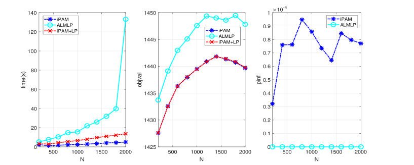
Figure 2: Numerical comparisons among iPAM, iPAM+LP and ALMLP for different $N$ with $m=60$

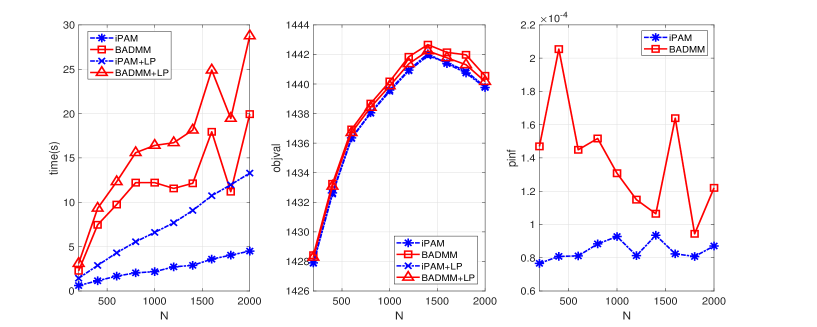
Figure 3: Numerical comparisons among iPAM, iPAM+LP, BADMM and BADMM+LP for different $N$ with $m=60$

Table 2: Average number of iterations of iPAM and BADMM corresponding to Figure 3

iter	$N$
(subiter)	$200$	$400$	$600$	$800$	$1000$	$1200$	$1400$	$1600$	$1800$	$2000$
PAM	35.6	35.7	35.4	35.2	33.6	34.5	33.0	34.3	34.6	34.4
	(328.6)	(280.4)	(301.1)	(278.3)	(232.4)	(250.2)	(226.2)	(255.3)	(254.9)	(258.3)
BADMM	2840	2720	2540	2420	2040	1680	1580	2080	1160	1900

Case 2. Influence of number of support points $m$ on three solvers.

We test the influence of $m$ on the performance of three solvers by using the example in Case 1. Figure 4 plots the average CPU time, objective value and infeasibility curves of iPAM, ALMLP and iPAM+LP under stcond A for $10$ independent tests, and Figure 5 plots the average CPU time, objective value and infeasibility curves of iPAM, BADMM, iPAM+LP and BADMM+LP under stcond B for $10$ independent tests. We see that iPAM requires less CPU time than ALMLP and BADMM do, and the objective values of its outputs are better than those yielded by ALMLP and BADMM. Similarly, the infeasibility yielded by ALMLP is the lowest, and the infeasibility of the output of iPAM is lower than that of the output of BADMM.

Table 3 reports the average number of iterations of iPAM and BADMM corresponding to Figure 5. We see that the average total number of iterations for the linearized ADMM is also much less than the average number of iterations of BADMM in this scenario.

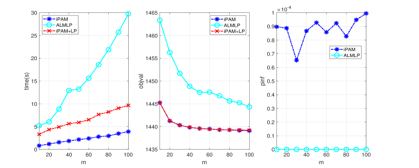
Figure 4: Numerical comparisons among iPAM, iPAM+LP and ALMLP for different $m$ with $N=1000$

Figure 5: Numerical comparisons of iPAM, BADMM, iPAM+LP and BADMM+LP for different $m$ with $N=1000$

Table 3: Average number of iterations of iPAM and BADMM corresponding to Figure 5

iter	$m$
(subiter)	$10$	$20$	$30$	$40$	$50$	$60$	$70$	$80$	$90$	$100$
iPAM	35.6	34.8	34.0	34.9	34.8	33.6	34.9	34.3	35.6	35.3
	(469.9)	(357.7)	(274.0)	(296.0)	(276.0)	(232.4)	(259.5)	(228.9)	(267.5)	(266.0)
BADMM	3000	3000	2080	2640	2560	2040	1840	1540	1400	1380

Case 3. Influence of the dimension of samples on three solvers.

To test the influence of $n_{t}$ on the performance of three solvers, we generate nine sets of $50$ discrete probability distributions with $N=50$ and $m=10$ for $n_{t}=400:400:3600$ in the same way as the paper YeWWL17 did, in which the support vectors are generated by sampling from a multivariate normal distribution and adding a heavy-tailed noise from the student’s t-distribution.

Figure 6 plots the average CPU time, objective value and infeasibility curves of iPAM, ALMLP and iPAM+LP under stcond A for $10$ independent tests, and Figure 7 plots the CPU time, objective value and infeasibility curves of iPAM, BADMM, iPAM+LP and BADMM+LP under stcond B for $10$ independent tests. We see that iPAM requires less CPU time than ALMLP and BADMM do, and the outputs of three solvers have comparable objective values. Similar to Case 1-2, the infeasibility yielded by ALMLP is the lowest, while that of BADMM is the highest.

Table 4 reports the average number of iterations of iPAM and BADMM corresponding to Figure 7. We see that the average total number of iterations for the linearized ADMM is less than that of BADMM, although now it is almost three times more than that of Case 1-2.

Figure 6: Numerical comparisons among iPAM, iPAM+LP and ALMLP for different $n_{t}$

Figure 7: Numerical comparisons among iPAM, BADMM, iPAM+LP and BADMM+LP for different $n_{t}$

Table 4: Average number of iterations of iPAM and BADMM corresponding to Figure 7

iter	$n_{t}$
(subiter)	$400$	$800$	$1200$	$1600$	$2000$	$2400$	$2800$	$3200$	$3600$
PAM	21.1	17.5	15.7	14.5	13.3	12.4	11.5	11.3	10.8
	(1586.5)	(1510.9)	(1479.7)	(1455.4)	(1444.2)	(1394.1)	(1377.1)	(1400.1)	(1363.7)
BADMM	3000	3000	3000	3000	3000	3000	3000	3000	3000

Case 4: Numerical performance on some real data.

In this part, we test the performance of three solvers on some real data described in Example 1-2 below.

Example 1

We obtain a set of 2225 discrete distributions from BBC News dataset that is divided into five classes. The average number of support points is about $25$ and the dimension of every support is $400$. The texts are treated as a bag of words, where the support vector is the vocabulary of the whole document and the weight corresponds to the appearing frequency of words.

Table 5 reports the numerical results of three solvers for Example 1, where the second row lists the results of iPAM under stcond B. We see that iPAM yields a little better objective values than ALMLP does within comparable CPU time, and it also yields comparable even a little better objective values than BADMM does within less one fifth of the CPU time of the latter. The objective values yielded by iPAM+LP are a little better than those of iPAM.

Example 2

We obtain a set of $11000$ discrete distributions from USPS Handwritten Digits which is divided into ten classes and the average number of support points is around $110$. The digit images are treated as normalized histograms over the pixel locations covered by the digits, where the support vector is the 2D coordinate of a pixel and the weight corresponds to pixel intensity.

Table 6 reports the numerical results of three solvers for Example 2, where the second row lists the results of iPAM under stcond B. We see that iPAM yields better objective values than ALMLP does within much less CPU time, and it yields comparable even better objective values than BADMM does within less CPU time. Similar to Table 5, the objective values given by iPAM+LP are a little better than those yielded by iPAM.

Example 3

We obtain a set of $10000$ discrete distributions from MNIST Handwritten Digits that is divided into ten classes and the average number of support points is around $151$. The digit images are treated as normalized histograms over the pixel locations covered by the digits, where the support vector is the 2D coordinate of a pixel and the weight corresponds to pixel intensity.

Table 7 reports the numerical results of three solvers for Example 3, where the second row lists the results of iPAM under stcond B. We see that iPAM yields better objective values than ALMLP does, its CPU time is at least less than one fifth of the CPU time of ALMLP, and it also yields comparable even better objective values than BADMM does within less CPU time. Similarly, the objective values given by iPAM+LP are a little better than those given by iPAM.

6 Conclusions

We have developed a globally convergent inexact PAM method for computing an approximate Wasserstein barycenter with unknown supports by designing a tailored linearized ADMM for solving the strongly convex QP subproblems. Numerical comparisons with the 3-block B-ADMM in YeWWL17 on synthetic and real data show that the proposed iPAM method has an advantage in reducing the computing time for large-scale problems while guaranteeing the quality of solutions. In our future research work, we will focus on the application of the iPAM method in the D2-clustering for image and document data.

Appendix

Algorithm 4 (D2-Clustering)

Initialization: Initialize the set of centroids $\{Q^{1,0},Q^{2,0},\ldots,Q^{K,0}\}$.
For $k=1,2,\ldots$ do

• for $t=1,2,\ldots,N$ do  (assignment step)

  $$l^{t,k}:=\mathop{\arg\min}_{s\in\{1,\ldots,K\}}W^{2}(Q^{s,k-1},P^{t})\qquad\qquad\qquad\qquad$$ (27)

  end for

• for $s=1,2,\ldots,K$ do  (optimization step)

  $$Q^{s,k}\in\mathop{\arg\min}_{Q}\sum_{l^{t,k}=s}\!W^{2}(Q,P^{t})\qquad\qquad\qquad\qquad$$ (28)

  end for

end For
Return the index set $\{l^{1,k},\ldots,l^{N,k}\}$ and the set of centroids $\{Q^{1,k},\ldots,Q^{K,k}\}$.

Table 5: Wasserstein Barycenters yielded by three solvers on BBC News dataset with $m=25$

	ALMLP		iPAM				iPAM+LP		BADMM				BADMM+LP
Class	time(s)	objval	time(s)	objval	pinf	iter(subiter)	time(s)	objval	time(s)	objval	pinf	iter	time(s)	objval
1	6.32	21.692	7.82	21.673	1.34e-4	32(695)	10.47	21.672	43.36	21.694	6.36e-4	3000	46.26	21.693
			8.01	21.673	7.91e-5	33(708)	10.54	21.672
2	11.25	10.336	6.71	10.331	9.58e-5	32(850)	8.97	10.330	33.06	10.329	4.23e-4	3000	35.44	10.329
			6.70	10.331	9.58e-5	32(850)	8.98	10.330
3	12.85	14.412	6.71	14.388	1.45e-4	32(741)	9.07	14.388	35.05	14.404	5.93e-4	3000	37.59	14.403
			7.41	14.388	8.50e-5	34(855)	9.82	14.388
4	14.73	9.827	8.44	9.807	7.61e-5	32(801)	11.32	9.806	42.69	9.815	4.88e-4	3000	46.05	9.814
			8.44	9.807	7.61e-5	32(801)	11.47	9.806
5	13.71	14.678	6.70	14.670	6.89e-5	32(800)	8.98	14.669	33.93	14.671	6.18e-4	3000	36.38	14.670
			6.71	14.670	6.89e-5	32(800)	9.10	14.669

Table 6: Wasserstein Barycenter yielded by three solvers on USPS dataset with $m=80$

	ALMLP		iPAM				iPAM+LP		BADMM				BADMM+LP
Class	time(s)	objval	time(s)	objval	pinf	iter(subiter)	time(s)	objval	time(s)	objval	pinf	iter	time(s)	objval
1	568.15	4.449	157.54	4.406	2.97e-5	27(1222)	198.31	4.404	286.15	4.408	1.19e-4	3000	332.22	4.408
			107.77	4.406	8.34e-5	21(835)	147.77	4.405
2	1014.28	4.832	204.65	4.810	3.24e-5	25(1275)	255.54	4.807	358.06	4.807	1.26e-4	3000	415.53	4.809
			142.71	4.812	1.00e-4	19(885)	193.67	4.809
3	774.08	4.060	210.88	4.042	3.17e-5	25(1290)	262.76	4.039	366.12	4.038	1.16e-4	3000	424.77	4.039
			158.35	4.044	8.50e-5	20(965)	210.39	4.040
4	705.05	4.133	166.99	4.096	2.96e-5	26(1204)	210.24	4.094	248.05	4.098	9.37e-5	2400	297.57	4.098
			111.23	4.098	8.74e-5	20(799)	154.36	4.095
5	957.64	4.595	196.15	4.563	3.89e-5	26(1313)	242.84	4.561	290.19	4.567	9.74e-5	2600	344.38	4.568
			143.69	4.565	7.41e-5	21(963)	190.70	4.562
6	1463.72	3.455	206.88	3.426	2.77e-5	25(1243)	259.75	3.423	374.02	3.427	1.16e-4	3000	433.69	3.427
			141.71	3.427	8.43e-5	19(848)	194.77	3.424
7	763.86	5.232	163.46	5.204	3.78e-5	26(1255)	203.91	5.199	291.78	5.208	1.91e-4	3000	337.73	5.209
			127.92	5.206	8.36e-5	22(971)	169.28	5.201
8	1305.74	3.557	224.56	3.500	2.72e-5	25(1293)	280.97	3.497	388.02	3.507	9.76e-5	3000	453.18	3.506
			152.55	3.501	9.97e-5	19(876)	209.39	3.498
9	1533.53	3.932	197.28	3.884	2.88e-5	25(1225)	248.87	3.881	359.36	3.887	1.00e-4	3000	417.12	3.887
			145.11	3.885	9.60e-5	20(897)	196.83	3.882
10	1056.10	2.037	223.14	2.002	2.85e-5	25(1237)	282.53	1.997	244.04	2.011	9.37e-5	1800	310.09	2.005
			137.45	2.003	9.66e-5	18(758)	196.81	1.999

Table 7: Wasserstein Barycenter yielded by three solvers on MNIST dataset with $m=160$

	ALMLP		iPAM				iPAM+LP		BADMM				BADMM+LP
Class	time(s)	objval	time(s)	objval	pinf	iter(subiter)	time(s)	objval	time(s)	objval	pinf	iter	time(s)	objval
1	4695.28	2.722	596.36	2.683	2.71e-5	23(1239)	786.62	2.678	724.51	2.687	8.16e-5	2200	922.39	2.681
			392.29	2.693	9.62e-5	17(810)	582.02	2.679
2	2776.96	2.831	274.07	2.793	3.23e-5	27(1071)	359.58	2.793	291.33	2.807	8.19e-5	1600	384.73	2.798
			178.27	2.800	9.46e-5	21(692)	264.29	2.794
3	5760.40	4.738	599.48	4.718	3.19e-5	24(1326)	775.90	4.711	885.09	4.714	7.85e-5	2800	1066.42	4.713
			408.40	4.720	9.04e-5	18(901)	581.10	4.712
4	4499.60	4.012	553.31	3.990	3.25e-5	24(1281)	716.81	3.983	717.42	3.986	9.53e-5	2400	891.34	3.986
			370.61	3.994	9.70e-5	18(860)	535.51	3.985
5	4172.91	3.912	434.40	3.877	2.95e-5	24(1184)	568.99	3.873	562.60	3.877	9.45e-5	2200	706.58	3.877
			310.87	3.878	9.06e-5	19(842)	445.72	3.874
6	4171.47	5.029	437.37	4.997	3.25e-5	24(1214)	572.74	4.993	557.75	4.995	9.54e-5	2200	703.30	4.997
			317.84	4.998	8.14e-5	19(878)	452.94	4.994
7	3914.88	3.672	516.11	3.647	2.75e-5	24(1269)	670.28	3.642	737.58	3.641	9.30e-5	2600	904.76	3.641
			354.05	3.648	8.61e-5	18(867)	507.92	3.643
8	5855.87	4.526	448.02	4.497	3.47e-5	25(1264)	575.95	4.492	698.46	4.494	9.16e-5	2800	835.29	4.491
			325.18	4.497	8.38e-5	20(912)	453.29	4.493
9	6308.66	3.230	552.55	3.193	2.38e-5	24(1231)	723.67	3.189	678.52	3.192	9.75e-5	2200	862.51	3.192
			345.52	3.201	9.47e-5	17(763)	516.48	3.190
10	5186.14	3.056	465.19	3.028	2.70e-5	24(1205)	604.51	3.026	643.69	3.032	9.08e-5	2400	795.67	3.030
			312.19	3.035	9.99e-5	18(807)	453.43	3.027