A measurement of the scintillation decay time constant of nuclear recoils in liquid xenon with the XMASS-I detector

Abstract

We report an in-situ measurement of the nuclear recoil (NR) scintillation decay time constant in liquid xenon (LXe) using the XMASS-I detector at the Kamioka underground laboratory in Japan. XMASS-I is a large single-phase LXe scintillation detector whose purpose is the direct detection of dark matter via NR which can be induced by collisions between Weakly Interacting Massive Particles (WIMPs) and a xenon nucleus. The inner detector volume contains 832 kg of LXe.

²⁵²Cf was used as an external neutron source for irradiating the detector. The scintillation decay time constant of the resulting neutron induced NR was evaluated by comparing the observed photon detection times with Monte Carlo simulations. Fits to the decay time prefer two decay time components, one for each of the Xe${}_{2}^{*}$ singlet and triplet states, with $\tau_{S}$ = 4.3$\pm$0.6 ns taken from prior research, $\tau_{T}$ was measured to be 26.9${}^{+0.7}_{-1.1}$ ns with a singlet state fraction F_S of 0.252${}^{+0.027}_{-0.019}$. We also evaluated the performance of pulse shape discrimination between NR and electron recoil (ER) with the aim of reducing the electromagnetic background in WIMP searches. For a 50% NR acceptance, the ER acceptance was 13.7${\pm}$1.0% and 4.1${\pm}$0.7% in the energy ranges of 5–10 keV_ee and 10–15 keV_ee, respectively.

1 Introduction

Liquid xenon (LXe) has been used in many modern experiments such as dark matter and neutrino-less double beta decay searches [1, 2, 3, 4, 5]. The scintillation timing information can be used for position reconstruction of an event in the detector [6] as well as for particle identification [7]. Studies on the scintillation process in LXe has been conducted in various experiments [8, 9, 10, 11, 12, 15, 16, 17, 18, 19, 13, 14]. A scintillation photon is produced by two mechanisms. One is the direct excitation of Xe atoms that then forms an excited dimer Xe${}_{2}^{*}$,

$$\mathrm{Xe}^{*}+\mathrm{Xe}+\mathrm{Xe} \rightarrow \mathrm{Xe}_{2}^{*}+\mathrm{Xe}~{},$$

$$\mathrm{Xe}_{2}^{*} \rightarrow 2\mathrm{Xe}+h\nu~{}.$$

The other process involves the recombination process between electrons and Xe ions

$$\mathrm{Xe}^{+}+\mathrm{Xe} \rightarrow \mathrm{Xe}_{2}^{+}~{},$$

$$\mathrm{Xe}_{2}^{+}+\mathrm{e}^{-} \rightarrow \mathrm{Xe}^{**}+\mathrm{Xe}~{},$$

$$\mathrm{Xe}^{**} \rightarrow \mathrm{Xe}^{*}+heat~{},$$

$$\mathrm{Xe}^{*}+\mathrm{Xe}+\mathrm{Xe} \rightarrow \mathrm{Xe}_{2}^{*}+\mathrm{Xe}~{},$$

$$\mathrm{Xe}_{2}^{*} \rightarrow 2\mathrm{Xe}+h\nu~{}.$$

The Xe${}_{2}^{*}$ dimer has both a singlet and triplet state, each with its own decay time constant. The decay time constants of the singlet and triplet states were reported to be 4.3$\pm$0.5 ns and 21$\pm$2 ns, respectively using ²⁵²Cf fission fragments [10]. While the recombination process has a longer decay time constant of more than 30 ns, measured with 1 MeV electrons from a ²⁰⁷Bi source [10, 11]. In the case of neutron induced NR events, the decay time constant of the triplet state was reported to be $\sim$20 ns both with an applied electric field (0.1–0.5 kV/cm) [13, 14] and without [15, 19]. The decay time constants of the singlet and triplet states depend weakly on the density of the excited species, whereas the ratio of the singlet to triplet state as well as the recombination time depends on the deposited energy density [20]. The time profile of events’ scintillation photon hits (pulse shape) may allow for discrimination between NR and ER initiated events [21].

XMASS-I is a large single phase LXe detector, built primarily for dark matter searches, previously reported the Xe${}_{2}^{*}$ triplet decay time constant of ER events using low energy gamma-rays calibration sources [8]. In this work, we measured the Xe${}_{2}^{*}$ triplet decay time constant of NR events using an external ²⁵²Cf neutron source irradiating the XMASS-I detector and also evaluated the usefulness of pulse shape discrimination (PSD) between NR and ER in the energy region of interest for dark matter searches.

2 Experimental apparatus

2.1 The XMASS-I detector

The XMASS-I detector is located in the Kamioka mine under 1,000 m of rock (2,700 meter water equivalent). As shown in Fig. 1, the inner detector (ID) contains 832 kg of LXe inside a spherical, oxygen free high conductivity (OFHC) copper structure with an 80 cm diameter. Scintillation light from the LXe is detected by 630 hexagonal R10789 photomultiplier tubes (PMTs) and 12 cylindrical R10789Mod PMTs with a total photocathode coverage of 62.4%. The inner containment vessel contains the LXe and the PMT holder, while the outer containment vessel holds vacuum for thermal insulation. In order to reduce external gamma-rays and neutrons from the surrounding rock, the ID is placed at the center of the outer detector (OD). The OD is a cylindrical tank 10 m in diameter and 11 m in height filled with ultrapure water. 72 Hamamatsu 20-inch R3600 PMTs are mounted on the inner surface of the water tank to provide an active muon veto. More details can be found in Ref. [1].

Signals from the 642 ID PMTs were recorded by CAEN V1751 waveform digitizers with a 1 GHz sampling rate and 10-bit resolution. Analog-timing-modules (ATMs) that were previously used in the Super-Kamiokande experiment [22, 23] worked for generating a trigger. The threshold for an ID PMT to register a hit in the ATMs is set at 0.2 photoelectron (PE). When 4 or more ID PMT hits are observed in a 200 ns coincidence window, a global trigger is issued to both the ATMs and the waveform digitizers. For each triggered event, the waveform is recorded with a width of 10 $\mu$s. The OD trigger requires at least 8 PMT hits in a 200 ns coincidence window.

2.2 Detector calibrations

2.2.1 LED calibration

The individual PMT gains are monitored by a blue LED embedded in the inner surface of the PMT holder. This LED is flashed every second using the one-pulse-per-second signal from the global positioning system. LED calibration data is taken continually during the physics runs and identified by the trigger information.

2.2.2 Energy calibration and light yield

To check the stability of the detector’s light yield, inner calibration data using a ⁵⁷Co source is taken every one or two weeks. Deploying the ⁵⁷Co 122 keV gamma-ray source at the center of the detector, we obtain a photoelectron yield of $\sim$15 PE / keV and also trace the timing offsets of the PMT channels. The ⁵⁷Co source as well as ⁵⁵Fe, ¹⁰⁹Cd, ²⁴¹Am, and ¹³⁷Cs are also measured off of center along the detector’s $z$-axis for position dependent energy calibration within the detector.

2.3 The neutron source and its deployment

²⁵²Cf undergoes spontaneous fission with a branching ratio of 3.11%. An average fission event emits 8 gamma-rays with a total energy of 7 MeV and 3.75 neutrons [24]. This gamma-ray emission is used to tag such fission events.

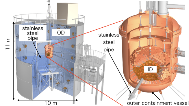
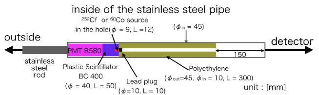
Figure 1: Schematic view of the XMASS detector and the calibration setup.

Figure 1 shows the calibration setup. To detect the gamma-rays, the ²⁵²Cf source was deployed in the cylindrical Bicron BC400 plastic scintillator, which is 40 mm in diameter, and 50 mm long. It has a central hole with a diameter of 9mm and a depth of 12 mm, in which the source is placed. The plastic scintillator was coupled with a Hamamatsu R580 1.5 inch PMT, and hereafter we call it a neutron tagging assembly (NTA). A timing calibration between the plastic scintillator and XMASS-I detector electronics was performed with the ⁶⁰Co source. The signal of the plastic scintillator was recorded by the same waveform digitizer used for the ID signals. A cylindrical polyethylene pipe with the outer diameter of 45 mm, the inner diameter of 10 mm, and the length of 300 mm was installed in front of the plastic scintillator and worked as a support structure. A 10 mm long lead plug is used to shield gamma-rays from the source. A stainless steel pipe, with a 45mm inner diameter passes through the water tank and terminates at 10 mm away from the outer containment vessel. This NTA was inserted into a stainless steel pipe. A stainless steel rod (SUS rod) attached to the NTA can position the NTA 150 mm away from the end of the stainless steel pipe. This distance is set so the detector trigger rate does not exceed 100 Hz; capable rate of the data acquisition (DAQ).

3 Analysis

3.1 Monte Carlo simulations

The XMASS Monte Carlo (MC) simulation is based on Geant4 [25]. It includes a detailed detector geometry, particle tracking, the Xe scintillation process, photon tracking, PMT response, and responses from the electronics. Table 1 summarises the input parameters used in the MC simulation. The optical parameters, such as the absorption and scattering length of LXe, are extracted by the comparison between data and MC simulation of the ⁵⁷Co calibrations at multiple source positions. Gamma-ray events originating close to the inner detector surface situated between PMTs was used to deduce the copper reflection by comparing the PE spectrum from observed data and MC simulation [6].

Table 1: Summary of input parameters used in the MC simulation. These were obtained by comparing observed data and MC simulations for a range of calibration techniques outlined above.

LXe density	2.89 g/cm3
Emission spectrum of LXe	Gaussian distribution (Ref. [26] )
	centered at 174.8 nm, FWHM 10.2 nm
Refractive index of LXe	1.58–1.72 for 183–167 nm
	from direct measurements [27] with a small correction
	considering density dependence
LXe absorption length	852.9 cm
LXe scattering length	52.7 cm
PMT average quantum efficiency	30%
PMT quartz absorption length	14.3 cm at 175 nm, measured by manufacturer
Copper reflectivity	25%

In the MC simulation of the ²⁵²Cf calibration, the Brunson model [24] and the Watt spectral model [28] were used for the input energy spectrum of the gamma-rays and the neutrons, respectively. A neutron can either be captured by a xenon nucleus or simply interact with it via elastic or inelastic scattering. The cross sections from both the ENDF/B-VII.0 library, and the G4NDL3.13 library based on the ENDF/B-VI library were used and the results compared in order to evaluate the cross section’s systematic uncertainty. We followed the instructions in Ref. [29, 30] to use ENDF/B-VII.0 library. In considering NR events, the relative scintillation efficiency L_eff [31], is defined as the scintillation yield of xenon for NR relative to the zero-field scintillation yield for 122 keV gamma-rays from ⁵⁷Co. The non-linearity of scintillation yield of ER events over energy was accounted for using a model from Ref. [32] tuned with XMASS-I gamma-ray calibration data. Using the measurement setup outlined in Fig. 1, the rate for multiple neutrons or gamma-rays from the same fission event to enter the ID simultaneously was found to be negligible. Therefore, only an individual neutron or gamma-ray was generated for each MC event in the ²⁵²Cf simulation with their intensities considered.

The detection time of the $i^{\rm th}$ photon $T^{i}$ after a ²⁵²Cf spontaneous fission is defined as

$$T^{i}=t_{\rm Edep}+t^{i}_{\rm scinti}+t^{i}_{\rm TOF}+t^{i}_{\rm TT}+t^{i}_{\rm jitter}.$$ (3.1)

$t_{\rm Edep}$ is the time when the incident particle deposits its energy in the LXe. And the LXe scintillation photon emission time $t^{i}_{\rm scinti}$ follows the scintillation decay time profile parameterized as

$$f(t)=\frac{F_{S}}{\tau_{S}}\cdot\mathrm{exp}\left(-\frac{t}{\tau_{S}}\right)+\frac{1-F_{S}}{\tau_{T}}\cdot\mathrm{exp}\left(-\frac{t}{\tau_{T}}\right).$$ (3.2)

We assumed that the scintillation decay time profile has two decay constants $\tau_{S}$ and $\tau_{T}$, corresponding to the decay constants of the singlet and the triplet states respectively, and that the fraction of photons generated from decays of singlet dimers $F_{S}$ and triplet dimers $F_{T}$ sum to unity ($F_{T}$ = 1 - $F_{S}$) following Ref. [8]. $t^{i}_{\rm TOF}$ is the time of flight (TOF) of the scintillation photon. Here, the group velocity of the scintillation light was calculated from the refractive index of LXe. $t^{i}_{\rm TT}$ is the transit time in the PMT, which we assume to be the same for all PMTs. The transit time spread (TTS) of $\sigma$ = 2.4 ns for PMT [33] was included in the timing calculation. $t^{i}_{\rm jitter}$ is a smearing parameter accounting for the timing jitter in the electronic channel of PMT and extracted from the ⁵⁷Co calibration data. It follows a Gaussian distribution with a standard deviation of 0.93 ns [8]. After calculating $T^{i}$ for all photons, a waveform for each PMT was simulated using the one PE pulse (template pulse) shape extracted from LED calibration data. A residual between the template pulse and the real data was found to be $\sigma$ < 0.1 PE for all PMTs.

3.2 Event selection

We took 1.5 hours of ²⁵²Cf source data with an ID trigger rate of roughly 80 Hz. The signal of the plastic scintillator was searched for by offline analysis. Events related to neutrons from the ²⁵²Cf source were selected using the following three criteria. (1) Only the ID trigger is issued to avoid muon or muon induced events. (2) The time difference from the previous ID event is longer than 500 $\mu$s and the root mean square of the timings of all hits in the event is less than 100 ns. This cut removes noise events that often follow particularly high energy events. (3) ID trigger is issued between 30 and 100 ns after the NTA trigger ($\Delta T$) to avoid ²⁵²Cf gamma-rays induced events. $\Delta T$ in MC simulation is calculated from the time difference between particle generation and an ID trigger being issued. Figure 2 shows the $\Delta T$ distributions of events which have less than 500 detected PE in the ID. The neutron in a MC event can deposit its energy at a single position or over multiple positions within the LXe. If all of the photons detected originate from a single position they are classed as single-site, if multiple positions then multi-site.

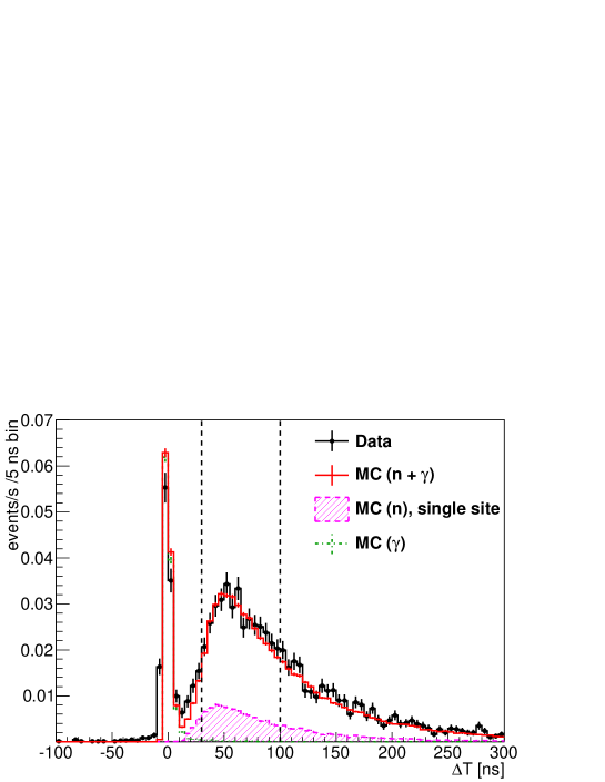
Figure 2: Timing distributions of ²⁵²Cf source data (solid black) and MC simulation (solid red). $\Delta T$ is defined in section 3.2. The timing of each event is aligned so that the events induced by the ²⁵²Cf gamma-rays peak at $\Delta T$ = 0 ns. Magenta dotted and green dash-dotted histograms show the timing distribution from the ²⁵²Cf neutron simulation (single site events only) and the ²⁵²Cf gamma-ray simulation, respectively. The accidental coincidence contribution was derived from the event rate in -1900 $<$ $\Delta T$ $<$ -100 ns time window. This accidental rate was about 3 $\times$ 10^-4 events/s and was subtracted from data. Events in 30 < $\Delta T$ < 100 ns were used for the NR events analysis.

Figure 3 shows the energy spectrum after all cuts. It includes the systematic uncertainties related to the detection efficiency of the plastic scintillator ($\pm$10%), the cross section difference between the G4NDL3.13 library and the ENDF-B/VII.0 library (25% at most), the scintillation efficiency for NR ($\pm$1$\sigma$ in Ref. [31], 10% at most). We observed a discrepancy (5% at most) in the mean observed PE between the ⁵⁷Co calibration data and MC simulation at large radii (>40 cm). This was included as a systematic uncertainty in the MC simulation in Fig. 3. The detection efficiency and tagging threshold of the plastic scintillator were estimated to be (70$\pm$10)% and 100 keV in gamma-ray energy, respectively, by comparing the data from ¹³⁷Cs and ⁶⁰Co to MC simulations using a small setup. The $\Delta T$ distribution of the MC simulation agreed with data as shown in Fig. 2. There was about 25% count rate difference below 20 detected PEs in the energy spectra in Fig. 3, we discuss its impact on the decay time constant in section 4.1.

Multi-site events make up about 75% of the neutron events as deduced from MC simulation. Events with PE counts between 10 and 100 PEs, corresponding to the energy range from 1.5 keV_ee (6.3 keV_nr) to 8.3 keV_ee (40 keV_nr), were used to evaluate the NR decay constant described in the following section.

Figure 3: Detected PE distributions of ²⁵²Cf source data (solid black) and MC simulation (solid red). The red band shows the quadratic sum of the systematic uncertainty and the statistical uncertainty of the MC simulation. The magenta hashed histogram and the green dash-dotted histogram show the single-site events from the ²⁵²Cf neutron simulation, ²⁵²Cf gamma-rays simulation, respectively. The contribution of the accidental coincidence events was derived from events in -1900 $<$ $\Delta T$ $<$ -100 ns time window and was subtracted from data. Events with PE counts between 10 and 100 PEs were used for NR events analysis.

3.3 Evaluation of the nuclear recoil decay time constant

The scintillation decay time constant of NR was evaluated by comparing the time-distributions of the detected PE over all PMTs and events between data and MC simulation with various timing parameters. To analyze waveforms of individual PMTs, we developed a peak finding algorithm based on a Savitzky-Golay filter [34] to obtain individual photon hit timings. Each peak was fitted with a single PE waveform template obtained from the LED calibration data. Figure 4 shows a NR event waveform from a single PMT with the fitting result. Due to fluctuations of the baseline and electronic noise, the peak-finding algorithm sometimes misidentifies the tail of the single PE distribution as a peak. Such misidentified peaks typically have PE smaller than 0.5 PE. In this study, only peaks that have more than 0.5 PE are used. For each event, all peaks from all PMTs are sorted in order of detected timings. The timing of the fourth earliest peak is set to $T$ = 0 ns with all other peak timings within the event shifted relative to this time, reflecting the trigger implementation in DAQ. This allows to superimpose all the recorded peak times over events.

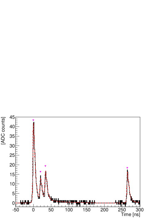
Figure 4: A raw waveform in a single PMT in a ²⁵²Cf calibration event. To reduce data size, parts of a waveform that do not exceed a threshold of 3 ADC counts were not recorded. The magenta triangles show the detected peaks. The dashed red line shows the waveform reconstruction obtained as the sum of each peak’s single-PE waveform fit. A typical single-PE pulse has a height of about 22.4 ADC counts after digitization.

To obtain the scintillation decay time constant for NR, we performed a $\chi^{2}$ fit defined as

$$\chi^{2}=\sum_{i}\frac{(N_{i}^{\rm data}-N_{i}^{\rm MC}\cdot S)^{2}}{\sigma_{\rm stat(\rm data)}^{2}+\sigma_{\rm stat(\rm MC)}^{2}\cdot S^{2}}~{},$$ (3.3)

where $N_{i}^{\rm data}$ and $N_{i}^{\rm MC}$ are the number of detected peaks in the $i^{\rm th}$ time bin over all of the data and simulated MC, respectively. $S$ is a free variable for normalization. $\sigma_{\rm stat(\rm Data)}$ and $\sigma_{\rm stat(\rm MC)}$ represent the statistical uncertainty in the data sample and the MC simulation, respectively.

The time bin width was 1 ns and the $\chi^{2}$ is calculated in the range of 3 $\leq T\leq$ 120 ns. To evaluate the scintillation decay time constant for NR, we scanned the parameter $F_{S}$ from 0.0 to 0.5 in steps of 0.025, and $\tau_{T}$ from 21.0 to 30.5 ns in steps of 0.5 ns in MC simulation. For $\tau_{S}$, we used 3.7, 4.3, and 4.9 ns taken from Ref. [10].

4 Result and discussion

4.1 The scintillation decay time constant of the nuclear recoil

Figure 5 shows the $\chi^{2}$ map in the $F_{S}$–$\tau_{T}$ plane. Since the parameters were scanned in discrete steps, a parabolic function fit as defined in Eq. 4.1 was performed to obtain the scintillation decay time constant.

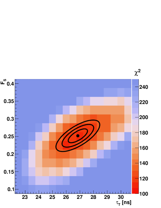
Figure 5: $\chi^{2}$ map in the $F_{S}$ and $\tau_{T}$ plane with $\tau_{S}$ = 4.3 ns. Black contours correspond to 1$\sigma$, 2$\sigma$, and 3$\sigma$ and are derived from a parabolic function fit described in Eq. 4.1. The black point of (26.9 ns, 0.252) for ($\tau_{T}$,$F_{S}$) is the best fit value from the parabolic function fit.

Figure 6: (Top) Pulse timing distributions of data (black) and the best fit MC simulation (red) ($\tau_{S}$,$\tau_{T}$,$F_{S}$) = (4.3 ns, 26.9 ns, 0.252). This MC distribution’s two components are also shown separately in green ($\tau_{T}$) and blue ($\tau_{S}$). (Bottom) The ratio of data to the best fit MC simulation.

$$\begin{split}\chi^{2}&=a\cdot(\tau_{T}^{\prime})^{2}+b\cdot(F_{S}^{\prime})^{2}+\chi^{2}_{\rm min}~{},{\rm where}\\ \tau_{T}^{\prime}&=(\tau_{T}-\tau_{T}^{\rm best})\cdot{\rm cos}\theta+(F_{S}-F_{S}^{\rm best})\cdot{\rm sin}\theta~{}{\rm and}\\ F_{S}^{\prime}&=-(\tau_{T}-\tau_{T}^{\rm best})\cdot{\rm sin}\theta+(F_{S}-F_{S}^{\rm best})\cdot{\rm cos}\theta~{}.\end{split}$$ (4.1)

Here $a$, $b$, $\chi^{2}_{\rm min}$, $\theta$, $\tau_{T}^{\rm best}$ and $F_{S}^{\rm best}$ are free parameters in the fit. The section of the parameter plane that has $\chi^{2}$ - $\chi^{2}_{\rm min}$ $<$ 20 in Fig. 5 was used for this fit. From this parabolic fit, ($\tau_{S}$, $\tau_{T}$, $F_{S}$) were discovered to be (4.3 ns, 26.9$\pm$0.5 ns (stat), 0.252$\pm$0.013 (stat)) with the minimum $\chi^{2}$ / ndf = 113.9 / 115. Data overlaid with the best fit MC simulation is shown in Fig. 6.

All systematic uncertainties are listed in Table 2. They were evaluated as follows:

Table 2: Summary of systematic uncertainties on $\tau_{T}$ and $F_{S}$.

Error source	$\sigma_{\tau_{T}}$ (ns)	$\sigma_{F_{S}}$
$\tau_{S}$	+0.5, -0.2	+0.009, -0.003
Neutron cross section	+0.2, -0.0	+0.006, -0.000
Leff	+0.0, -0.7	+0.019, -0.010
Jitter	+0.1, -0.2	+0.009, -0.010
After/Pre-pulse	+0.0, -0.6	+0.000, -0.001
Total	+0.5, -1.0	+0.024, -0.014

(1)$\tau_{S}$: $\tau_{S}$ = 4.3$\pm$0.6 ns from Ref. [10] was used in this analysis. The systematic uncertainty introduced by $\tau_{S}$ was evaluated by changing $\tau_{S}$ from 4.3 ns to 3.7 ns and 4.9 ns.

(2)Neutron cross section: the event rate, including the fraction of multi-site events, depends on the neutron cross-section. We found an event rate difference of about 10% between the MC simulation using the ENDF-B/VII.0 and the MC simulation using the G4NDL3.13 library. Parameter scans of $F_{S}$ and $\tau_{T}$ with the G4NDL3.13 library were conducted, and the difference of the respective best fit value was used as the systematic uncertainty due to the neutron cross section. The effect of the count rate difference mentioned in section 3.2 was also evaluated. We evaluated the impact on the scintillation decay time constant by lowering the weight of events in the data below 20 PEs and it turned out to be a negligible effect.

(3)L_eff: following Ref. [31]’s error estimates, we ran MC simulations also with L_eff $\pm$1 $\sigma$. We used the difference of the respective best fit values as the systematic uncertainty due to L_eff.

(4)Jitter: timing jitter affects the determination of the rising edge of timing distributions. The uncertainty was evaluated by comparing the timing distribution of data and simulated samples with different assumptions for the amount of timing jitter. $t_{\rm jitter}$ was changed from $\sigma$ = 0.93 ns to 0.0, 0.5, 1.5 ns and the differences of the respective best fit value were assigned as systematic uncertainty.

(5)After-pulse and pre-pulse: occasionally single-PE pulses are observed prior to or after the main event pulse, these are aptly labeled pre-pulses and after-pulses, respectively. Their rate and timing information was measured independently in a laboratory setup. The pre-pulses were found to have a 0.10% /PE probability of occurring and on average are located $\sim$15 ns before the main pulse in a time width of $\sim$2 ns. After-pulses have a probability of 0.65% /PE and are located $\sim$40 ns after in a time width of $\sim$5 ns. To study their impact, we generated single-PE pulse timings at the appropriate rate using a Gaussian distribution centered at 40 ns with a 5 ns width and another at -15 ns with a 2 ns width for the after-pulses and pre-pulses, respectively. The differences of the best fit values between using the standard MC PE pulse times and these same times augmented with generated pre-pulse and after-pulse times is used for their systematic uncertainty.

After adding these systematic uncertainties in quadrature, the scintillation decay time constant for NR was estimated to be ($\tau_{T}$, $F_{S}$) = (26.9$\pm$0.5 (stat)${}^{+0.5}_{-1.0}$ (sys) ns , 0.252$\pm$0.013 (stat)${}^{+0.024}_{-0.014}$ (sys)) with $\tau_{S}$ = 4.3$\pm$0.6 ns.

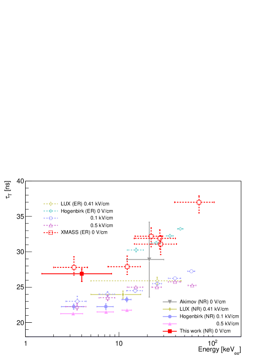
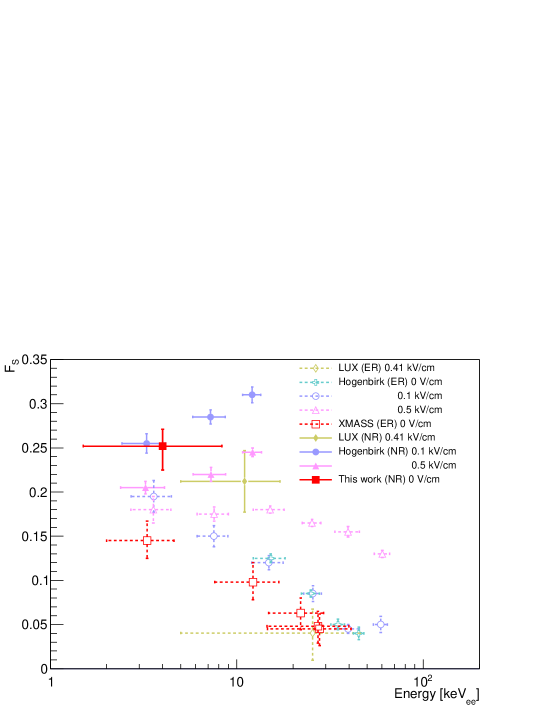
Figure 7: The best-fit parameters $\tau_{T}$ and F_S for various measurements. Filled markers and solid lines correspond to NR measurements. Open markers and dotted lines correspond to ER measurements. Results from Akimov et al. [15], Teymourian et al. [17], the LUX experiment [13], Hogenbirk et al. (0 V/cm, 0.1 kV/cm and 0.5 kV/cm) [14], and XMASS measurement (This work and [8]) are indicated by the black triangle, cyan cross, yellow diamond, green cross, blue circle, magenta triangle, and red square, respectively.

The obtained $\tau_{T}$ is close to that for ER (27.8${}^{+1.5}_{-1.1}$ ns using ⁵⁵Fe 5.9 keV gamma-rays ) reported in Ref. [8], although the obtained $F_{S}$ is larger than that of ER (0.145${}^{+0.022}_{-0.020}$ using ⁵⁵Fe 5.9 keV gamma-ray). Figure 7 shows $\tau_{T}$ and F_S for various NR and ER measurements. This measurement had the lowest energy threshold of all the experiments conducted without an external electric field. D. Akimov et al. reported a scintillation decay time constants using a single component exponential fit [15]. The single component fit value of $\tau$ = 22.5 ns for 1.5 < E < 8.3 keV_ee in this work is close to their reported value, although the MC simulation does not reproduce the data well ($\chi^{2}$ / ndf = 368.1 / 116 ). The singlet fraction obtained in this work agrees with the results of Ref. [13, 14], however, the $\tau_{T}$ is about 5 ns longer than those values. The $\tau_{T}$ discrepancy might stem from a time delay introduced by the recombination process, which is suppressed under an electric field. The recombination process contributes at most 10% of total scintillation light for nuclear recoil [35]. For alpha particles and ²⁵²Cf fission fragments, this process is thought to be very fast and also have only a minor influence, for these species $\tau_{T}$ was reported as 22$\pm$1.5 ns and 21$\pm$2 ns, respectively [10] without an applied electric field.

4.2 Performance of the pulse shape discrimination

For Weakly Interacting Massive Particle (WIMP) searches in data from a single phase LXe detector, the possibility of PSD between NR and ER is of significant interest. We evaluated the performance of PSD in XMASS-I based on our scintillation decay time constant measurement. To obtain the relevant timing distributions, we first simulated the ER events with uniform energy from 0 to 20 keV and NR events which followed the energy distribution of 100 GeV/c² WIMPs elastically scattering in the LXe target at the center of the detector. Figure 8 shows the peak timing distributions of those simulated ER and NR events that had energy deposits from 5 to 10 keV_ee. In Fig. 8, TOF was subtracted using the velocity of 110 mm/ns for light in LXe and the timing of the fourth earliest peak in each event was set to $T$ = 0 ns again to reflect the trigger implementation in DAQ. As mentioned in section 4.1, F_S in NR is larger than in ER. Therefore a difference in the timing distributions can clearly be seen. These histograms in Fig. 8 were used as the probability density function ($f_{\rm ER,NR}(t_{i}$)) of the PMTs hit timings and we evaluated the following log likelihood ratio

$$\ln\left(\frac{{L}_{\rm NR}}{{L}_{\rm ER}}\right)=\sum\ln(f_{\rm NR}(t_{i}))-\sum\ln(f_{\rm ER}(t_{i}))~{}.$$ (4.2)

This log likelihood ratio was calculated using PMT hit times T > 0 ns, after TOF subtraction and T₀ determination. TOF subtraction uses the reconstructed event position. The performance of this PSD method was evaluated using another MC simulation. Electron events and NR events where simulated with the same energy distributions as before, but now generated uniformly throughout the detector. Figure 9 shows the log likelihood ratio distribution of the simulated ER and NR events that have energy deposits from 5 to 10 keV_ee and were reconstructed within 20 cm from the detector center, these events were used for the evaluation of the PSD performance.

The ER acceptances when requiring a 50% NR acceptance for energies between 5 to 10 keV_ee and between 10 to 15 keV_ee were estimated to be 13.7${\pm}$1.0% and 4.1${\pm}$0.7%, respectively. This corresponds to a S/$\sqrt{\rm N}$ ratio of 1.4 and 2.5, respectively. In Fig. 10 the blue curve shows the ER acceptance as a function of energy. The performance of this PSD method when evaluated using the XMASS-I detector simulation is consistent with the performance that we reported previously using a small chamber [21]. We also evaluated the performance of this PSD in an ideal case where the measurement is not affected by the timing jitter or TTS (red curve in Fig. 10). In this ideal case, the PSD performance improves by about a factor of 2 between 5 and 7 keV_ee, and by about one order of magnitude between 15 and 20 keV_ee.

Figure 8: Pulse timing distribution of the simulated ER and NR events with energy deposition from 5 to 10 keV_ee. In this figure, TOF was subtracted and the timing of the fourth earliest peak in each event was shifted to T=0 ns to reflect the trigger implementation. Areas are normalized to 1.

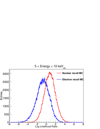
Figure 9: Log likelihood ratio distributions of simulated ER (blue) and NR events (red) reconstructed within a 20 cm radius from the detector center. A positive (negative) log likelihood ratio corresponds to NR (ER) like events.

5 Conclusions

We evaluated the time profile of NR scintillation emission in LXe with the XMASS-I detector using ²⁵²Cf sources. Two decay components are needed to reproduce the timing distribution of the NR data. We obtained the decay time constant of triplet state $\tau_{T}$ = 26.9$\pm$0.5 (stat)${}^{+0.5}_{-1.0}$ (sys) ns and the singlet fraction F_S = 0.252$\pm$0.013 (stat)${}^{+0.024}_{-0.014}$ (sys) with a decay time constant of singlet state $\tau_{S}$ = 4.3$\pm$0.6 ns taken from a prior research. This measurement had the lowest energy threshold without an aplied electric field. We also developed a PSD method based on a log likelihood ratio. The ER acceptances with a 50% NR acceptance at energies between 5 and 10 keV_ee and between 10 and 15 keV_ee were estimated to be 13.7${\pm}$1.0% and 4.1${\pm}$0.7%, respectively.

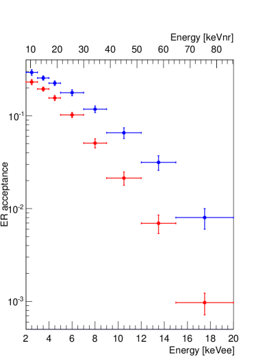
Figure 10: ER acceptance as a function of energy. NR equivalent energy is indicated on the top scale. WIMPs with a mass of 100 GeV/c² were used in the NR simulation. Electrons with energy distributed uniformly between 0 and 20 keV were used in the ER simulation. Both MC simulations generated uniformly distributed events within the XMASS-I detector and events which were reconstructed within 20 cm from the detector center were used for the evaluation. The two curves correspond to the log likelihood performance evaluated for a 50% NR acceptance. Error bars show the quadratic sum of systematic uncertainty and statistical uncertainty. The blue curve shows the result of XMASS-I detector, and the red one represents an ideal case where measurements are not affected by timing jitter in the electronics and TTS in the PMTs.

References

- [1] K. Abe et al. [XMASS Collaboration], “XMASS detector,” Nucl. Instrum. Meth. A 716 (2013) 78 [arXiv:1301.2815 [physics.ins-det]].
- [2] D. S. Akerib et al. [LUX Collaboration], “The Large Underground Xenon (LUX) Experiment,” Nucl. Instrum. Meth. A 704 (2013) 111 [arXiv:1211.3788 [physics.ins-det]].
- [3] X. Cao et al. [PandaX Collaboration], “PandaX: A Liquid Xenon Dark Matter Experiment at CJPL,” Sci. China Phys. Mech. Astron. 57 (2014) 1476 [arXiv:1405.2882 [physics.ins-det]].
- [4] E. Aprile et al. [XENON Collaboration], “The XENON1T Dark Matter Experiment,” Eur. Phys. J. C 77 (2017) no.12, 881 [arXiv:1708.07051 [astro-ph.IM]].
- [5] M. Auger et al. [EXO Collaboration], “The EXO-200 detector, part I: Detector design and construction,” JINST 7 (2012) P05010 [arXiv:1202.2192 [physics.ins-det]].
- [6] K. Abe et al. [XMASS Collaboration], “A direct dark matter search in XMASS-I,” arXiv:1804.02180 [astro-ph.CO].
- [7] K. Abe et al. [XMASS Collaboration], “Improved search for two-neutrino double electron capture on 124Xe and 126Xe using particle identification in XMASS-I,” PTEP 2018, no. 5, 053D03 (2018) [arXiv:1801.03251 [nucl-ex]].
- [8] H. Takiya et al. [XMASS Collaboration], “A measurement of the time profile of scintillation induced by low energy gamma-rays in liquid xenon with the XMASS-I detector,” Nucl. Instrum. Meth. A 834 (2016) 192 [arXiv:1604.01503 [physics.ins-det]].
- [9] S. Kubota, M. Hishida and J. Raun, “Evidence for a triplet state of the self-trapped exciton states in liquid argon, krypton and xenon,” J. Phys. C 11 (1978) 2645.
- [10] A. Hitachi, T. Takahashi, N. Funayama, K. Masuda, J. Kikuchi and T. Doke, “Effect of ionization density on the time dependence of luminescence from liquid argon and xenon,” Phys. Rev. B 27 (1983) 5279.
- [11] S. Kubota et al., “Dynamical behavior of free electrons in the recombination process in liquid argon, krypton, and xenon,” Phys. Rev. B 20 (1979) 3486.
- [12] J. W. Keto et al., “Exciton lifetimes in electron beam excited condensed phases of argon and xenon,” J. Chem. Phys. 71 (1979) 2676.
- [13] D. S. Akerib et al. [LUX Collaboration], “Liquid xenon scintillation measurements and pulse shape discrimination in the LUX dark matter detector,” Phys. Rev. D 97 (2018) no.11, 112002 [arXiv:1802.06162 [physics.ins-det]].
- [14] E. Hogenbirk, J. Aalbers, P. A. Breur, M. P. Decowski, K. van Teutem and A. P. Colijn, “Precision measurements of the scintillation pulse shape for low-energy recoils in liquid xenon,” JINST 13 (2018) no.05, P05016 [arXiv:1803.07935 [physics.ins-det]].
- [15] D. Akimov et al., “Measurements of scintillation efficiency and pulse shape for low-energy recoils in liquid xenon,” Phys. Lett. B 524 (2002) 245 [hep-ex/0106042].
- [16] J. V. Dawson et al., “A study of the scintillation induced by alpha particles and gamma rays in liquid xenon in an electric field,” Nucl. Instrum. Meth. A 545 (2005) 690 [physics/0502026].
- [17] A. Teymourian et al., “Characterization of the QUartz Photon Intensifying Detector (QUPID) for Noble Liquid Detectors,” Nucl. Instrum. Meth. A 654 (2011) 184 [arXiv:1103.3689 [physics.ins-det]].
- [18] I. Murayama and S. Nakamura, “Time profile of the scintillation from liquid and gaseous xenon,” Nucl. Instrum. Meth. A 763 (2014) 533.
- [19] K. Ueshima Ph. D. Thesis, The University of Tokyo, Tokyo, Japan (2010).
- [20] E. Aprile and T. Doke, “Liquid Xenon Detectors for Particle Physics and Astrophysics,” Rev. Mod. Phys. 82, 2053 (2010) [arXiv:0910.4956 [physics.ins-det]].
- [21] K. Ueshima et al. [XMASS Collaboration], “Scintillation-only Based Pulse Shape Discrimination for Nuclear and Electron Recoils in Liquid Xenon,” Nucl. Instrum. Meth. A 659 (2011) 161 [arXiv:1106.2209 [physics.ins-det]].
- [22] H. Ikeda, M. Mori, T. Tanimori, K. i. Kihara, Y. Suzuki and Y. Haren, “Front end hybrid circuit for Super-Kamiokande,” Nucl. Instrum. Meth. A 320 (1992) 310.
- [23] Y. Fukuda et al. [Super-Kamiokande Collaboration], “The Super-Kamiokande detector,” Nucl. Instrum. Meth. A 501 (2003) 418.
- [24] T. E. Valentine, “Evaluation of prompt fission gamma rays for use in simulating nuclear safeguard measurements,” Ann. Nucl. Eng. 28 (2001) 191.
- [25] S. Agostinelli et al. [GEANT4 Collaboration], “GEANT4: A Simulation toolkit,” Nucl. Instrum. Meth. A 506 (2003) 250.
- [26] K. Fujii et al., “High-accuracy measurement of the emission spectrum of liquid xenon in the vacuum ultraviolet region,” Nucl. Instrum. Meth. A 795 (2015) 293.
- [27] S. Nakamura et al., Measurements of optical properties of liquid xenon scintillator. In Proceedings of Workshop on Ionization and Scintillation Counters and Their Uses, Waseda University (2007) 27.
- [28] F. H. Fröhner, Evaluation of 252Cf Prompt Fission Neutron Data from 0 to 20 MeV by Watt Spectrum Fit, Nucl. Sci. Eng. 106 (1990) 345.
- [29] E. Mendoza, D. Cano-Ott, C. Guerrero and R. Capote, “New Evaluated Neutron Cross Section Libraries for the GEANT4 Code,” IAEA technical report INDC(NDS)-0612 (2012).
- [30] E. Mendoza, D. Cano-Ott, T. Koi and C. Guerrero, “New Standard Evaluated Neutron Cross Section Libraries for the GEANT4 Code and First Verification,” IEEE Trans. Nucl. Science 61 (2014) 2357.
- [31] E. Aprile et al. [XENON100 Collaboration], “Dark Matter Results from 100 Live Days of XENON100 Data,” Phys. Rev. Lett. 107 (2011) 131302 [arXiv:1104.2549 [astro-ph.CO]].
- [32] T. Doke et al., in Proceedings of the International Workshop on Technique and Application of Xenon Detectors (Xenon 01), World Scientific 17 (2003).
- [33] H. Uchida et al. [XMASS Collaboration], “Search for inelastic WIMP nucleus scattering on 129Xe in data from the XMASS-I experiment,” PTEP 2014 (2014) no.6, 063C01 [arXiv:1401.4737 [astro-ph.CO]].
- [34] A. Savitzky and M. J. E. Golay, “Smoothing and Differentiation of Data by Simplified Least Squares Procedures,” Anal. Chem. 36 (8) (1964) 1627.
- [35] E. Aprile et al., “Simultaneous measurement of ionization and scintillation from nuclear recoils in liquid xenon as target for a dark matter experiment,” Phys. Rev. Lett. 97 (2006) 081302 [astro-ph/0601552].