Analytical nonlinear collisional dynamics of near-threshold eigenmodes
Abstract
A closed-form analytical solution is found for the nonlinear dynamics of isolated, near-threshold waves in the presence of strong scattering. The proposed solution can be useful in verifying codes across several disciplines, including Alfvénic instabilities and thermal plasma turbulence in fusion plasmas and studies of viscous shear flows in fluid dynamics, as well as a rapid means for predicting and analyzing experimental outcome.
The obtention of reliable bounds for the nonlinear instability of waves is an outstanding problem in kinetic systems of fusion interest (Gorelenkov et al., 2014; Chen and Zonca, 2016). The burning plasma sustainment in ITER imposes severe constraints on the amount of fast ions ejected through their resonant interaction with Alfvénic waves (ITER Physics Expert Group on Energetic Particles, Heating and Current Drive and ITER Physics Basis Editors, 1999). Therefore, procedures to anticipate the nonlinear evolution of waves destabilized by the sub-population of highly energetic particles are needed for establishing limits for wave growth in ITER as well as in present tokamaks. In this letter, we derive an analytical expression for nonlinear wave evolution in the presence of strong scattering that can be a rapid means for experimental prediction and interpretation, as well as for the verification of codes.
The nonlinear dynamics of a non-overlapping wave near marginal stability has been found to be governed by a universal111The same equation can be recovered for the evolution of a mode in a turbulent plasma under a geometric optics approximation, i.e., when the turbulent modes can be treated as quasi-particles (Mendonça et al., 2014). A time-delayed, cubic equation of the same structure was also found in studies of critical layers in shear fluid flows (Hickernell, 1984). time-delayed, integro-differential cubic equation which, in the presence of diffusive processes, reads (Berk et al., 1996; Breizman et al., 1997)
| (1) |
where represents the effective scattering frequency normalized with ( is the linear growth rate in the absence of damping and is the sum of a wave background damping rates due to several mechanisms). Time is also normalized with . is an effective frequency due a combination of stochastic processes experienced by the resonant population, e.g., collisional pitch-angle scattering, collisionless turbulent scattering and diffusion due to RF heating waves. The normalized amplitude is , where is the bounce (or trapping) frequency of the most deeply trapped resonant particles222For a simplified bump-on-tail electrostatic case, is given by with , and being the resonant particle electric charge, the absolute value of the wave number vector and the resonant particle mass. For a more realistic toroidal configuration, is given by eq. 9 of (Berk et al., 1997). We note that if our results are to be compared with the ones of Ref. (Berk et al., 1997), our amplitude would need to be divided by a factor , since that reference used a slightly modified normalization.. is a phase-space volume element and is a phase-space weighting defined in (Berk et al., 1997; Duarte et al., 2017a).
Previous numerical analysis for Alfvénic modes in DIII-D, NSTX and TFTR (Duarte et al., 2017b, a) have shown that the phase average, over multiple mode resonance surfaces, leads to typical effective collisional scattering frequency of order to . Anomalous scattering (Lang and Fu, 2011) as well as diffusion due to radiofrequency heating (Bergkvist et al., 2005) contribute to increase the effective scattering rate. The net growth rate is typically of order of up to a percent of the wave frequency (the frequecy of toroidicity-induced and reversed-shear Alfvénic eigenmodes is typically of order ). Therefore, regimes with are relevant for experiments, especially when the modes are close to threshold and when diffusive mechanisms, in addition to collisions, are taken into consideration333In the context of (Mendonça et al., 2014), this limit is equivalent to very high damping rates of turbulent modes while in the context of (Hickernell, 1984) it translates into highly viscous shear flows..
For large scattering frequency, memory effects are easily destroyed as resonant particles receive frequent random kicks, and only the very recent history dictates the wave dynamics. For , the integral kernel makes the nonlinear term be zero at all times except when both and are close to zero. For very small and , the kernel of Eq. (1) changes much faster than the arguments of the amplitudes in the cubic term and the term in the curly brackets can be written as . The argument of the first exponential approaches zero faster than the one of the second exponential, therefore it is the term that gives the most important contribution. By redefining the variable of integration as , the resulting integral can be written as . We can then seek an analytical solution of the resulting equation
| (2) |
by dividing it by and defining an auxiliary variable . Assuming , a closed-form result is444In terms of the trapping frequency, the solution is where . In this expression the time variable is the actual time multiplied by . The average over the resonance surfaces is defined by , where is an element of phase space and , as defined in (Gorelenkov et al., 1999)
| (3) |
where is the initial amplitude and . Eq. (3) is consistent with its expected asymptotic behaviors since (i) for , when the cubic term is unimportant, the mode grows linearly, i.e., provided that and (ii) for , the saturation level is (the sign depends on whether is positive or negative). Using the amplitude normalization adopted for Eq. (1) we find that, under a bump-on-tail simplification, this correponds to the saturation level , which agrees with the one previously reported in (Berk et al., 1997; Petviashvili, 1997). To the best of our knowledge, Eq. (3) is the first analytical solution for the mode amplitude evolution, from a seed level up to saturation, in the presence of collisions.555An explosive solution (Berk et al., 1996) for the cubic equation (1) has been obtained for the situation in which the linear term is disregarded and the kernel can be replaced by the unity. The latter signals the breakdown of the theory validity.
The associated nonlinear growth rate can be calculated from , which gives
| (4) |
For experimental purposes, it can be useful to anticipate the timescale for mode saturation, as a function of and the initial amplitude . For that purpose, one can gain insights by analyzing the inflection time point of the solution (3), which is
| (5) |
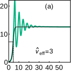
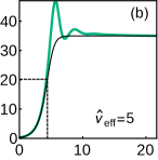
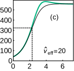
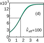
and corresponds to a characteristic amplitude of . The inflection is indicated on Fig. 1.
In Fig. (1), we compare the solution for , Eq. (3), with the full time-delayed cubic equation, Eq. (1), for different values of . We observe that Eq. (3) describes the trace of the wave amplitude reasonably well for , which is when the full cubic equation admits a steady solution (Breizman et al., 1997; Heeter et al., 2000). The assumption of high used to derive the analytical solution therefore turns out to be less restrictive than anticipated. In fact, simply needs to be high enough to ensure steady saturation, i.e., to prevent the emergence of wave chirping as well as other higher-order nonlinear bifurcations.
The existence of a steady solution is always allowed in Eq. (2) since the linear term can in principle balance the cubic term. The stability of solution (3) can be addressed via eigenvalue analysis by substituting in Eq. (2) a perturbed solution in the form , with . The result is and , which means that the saturated solution is intrinsically stable: any linear perturbation will exponentially asymptote to the saturation level, without the possibility of oscillations, which are suppressed by strong scattering processes.
We note that if the collisional scattering kernel of eq. (1), , were substituted by a Krook-type kernel ( is the Krook collisional frequency normalized with ), then solutions of the same type of eq. (3), (4) and (5) are admitted, with the transformation . For the Krook case, the saturation level implied by the analytical solution is , in agreement with (Berk et al., 1996).
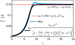
Eqs. (3) and (4) can be used as a verification for codes, e.g., quasilinear (Gorelenkov et al., 2018; Liu et al., 2018), gyrofluid (Spong et al., 1994), gyrokinetic (Lin et al., 1998; Lauber et al., 2007; Bass and Waltz, 2010; Zarzoso et al., 2012; Wilkie et al., 2015; Bass and Waltz, 2017; Biancalani et al., 2017; Slaby et al., 2018; Cole et al., 2018), hybrid (gyro-)kinetic/MHD (Fu and Park, 1995; Briguglio et al., 1995; Todo and Sato, 1998; Lang et al., 2010; Wang and Briguglio, 2016; Wang et al., 2016; Chen et al., 2018; Briguglio et al., 2017), kinetic (Lesur et al., 2010; Lilley et al., 2010; Woods et al., 2018; Li et al., 2018) and guiding-center following (Pinches et al., 1998; Chen et al., 1999; Gorelenkov et al., 1999; Zhou and White, 2016; White et al., 2016) simulations for the situation in which the amplitude of a marginally unstable wave evolves towards a quasi-steady satuaration. Another possibility to explore the analytical solution 3 is to compute the distribution function folding within the cubic equation framework, as recently numerically demonstrated (Sanz-Orozco et al., 2018). A high scattering frequency used in this work destroys phase-space correlations and therefore prevents the emergence of highly nonlinear scenarios, such as wave chirping and avalanching. Quasilinear theory employs a similar reasoning since it neglects the ballistic fast-oscillating term in its derivation, thereby also not capturing fully nonlinear wave behavior. An example of the comparison between Eq. 3 and the RBQ code (Gorelenkov et al., 2018) is shown in Fig. 2, which show fair agreement for regions of parameters where RBQ does not admit intermittent solutions.
If collisionality is moderate, we note that an amplitude overshoot occurs following the linear phase, as can be seen from Fig. 1(a). This can lead to instantaneous wide resonance islands (the resonance width is roughly proportional to (Meng et al., 2018) and therefore proportional to ). The overshoot can be several times the saturated amplitude, as shown in (Zhou and White, 2016). This may lead to instantaneous overlap of distinct resonances and invalidate/breaks down the analysis within the cubic equation framework. Therefore, for purposes of code verification, the expression 3 applies when collisions are high enough to ensure a monotonic saturation, in addition to the near threshold regime. As a final remark, we point out that higher-order nonlinear effects not considered in this work, such as MHD nonlinearities (Zonca et al., 1995) and wave-wave coupling (Hahm and Chen, 1995; Qiu et al., 2018) can establish further bounds on the saturation level.
Acknowledgements.
This work was supported by the US Department of Energy (DOE) under contract DE-AC02-09CH11466. The authors thank V. L. Quito and H. L. Berk for several discussions.?refname?
- Gorelenkov et al. (2014) N. Gorelenkov, S. Pinches, and K. Toi, Nucl. Fusion 54, 125001 (2014).
- Chen and Zonca (2016) L. Chen and F. Zonca, Rev. Mod. Phys. 88, 015008 (2016).
- ITER Physics Expert Group on Energetic Particles, Heating and Current Drive and ITER Physics Basis Editors (1999) ITER Physics Expert Group on Energetic Particles, Heating and Current Drive and ITER Physics Basis Editors, Nuclear Fusion 39, 2471 (1999).
- Mendonça et al. (2014) J. T. Mendonça, R. M. O. Galvão, and A. I. Smolyakov, Plasma Physics and Controlled Fusion 56, 055004 (2014).
- Hickernell (1984) F. J. Hickernell, J. Fluid Mech. 142, 431 (1984).
- Berk et al. (1996) H. L. Berk, B. N. Breizman, and M. Pekker, Phys. Rev. Lett. 76, 1256 (1996).
- Breizman et al. (1997) B. N. Breizman, H. L. Berk, M. S. Pekker, F. Porcelli, G. V. Stupakov, and K. L. Wong, Phys. Plasmas 4, 1559 (1997).
- Berk et al. (1997) H. L. Berk, B. N. Breizman, and M. Pekker, Plasma Phys. Rep. 23, 778 (1997).
- Duarte et al. (2017a) V. N. Duarte, H. L. Berk, N. N. Gorelenkov, W. W. Heidbrink, G. J. Kramer, R. Nazikian, D. C. Pace, M. Podestà, and M. A. V. Zeeland, Physics of Plasmas 24, 122508 (2017a), https://doi.org/10.1063/1.5007811 .
- Duarte et al. (2017b) V. N. Duarte, H. L. Berk, N. N. Gorelenkov, W. W. Heidbrink, G. J. Kramer, R. Nazikian, D. C. Pace, M. Podestà, B. J. Tobias, and M. A. V. Zeeland, Nuclear Fusion 57, 054001 (2017b).
- Lang and Fu (2011) J. Lang and G.-Y. Fu, Phys. Plasmas 18, 055902 (2011).
- Bergkvist et al. (2005) T. Bergkvist, T. Hellsten, T. Johnson, and M. Laxaback, Nuclear Fusion 45, 485 (2005).
- Gorelenkov et al. (1999) N. N. Gorelenkov, Y. Chen, R. B. White, and H. L. Berk, Phys. Plasmas 6, 629 (1999).
- Petviashvili (1997) N. Petviashvili, Coherent structures in nonlinear plasma dynamics, Ph.D. thesis, University of Texas, Austin (1997).
- Heeter et al. (2000) R. F. Heeter, A. F. Fasoli, and S. E. Sharapov, Phys. Rev. Lett. 85, 3177 (2000).
- Berk et al. (1995) H. Berk, B. Breizman, J. Fitzpatrick, and H. Wong, Nucl. Fusion 35, 1661 (1995).
- Ghantous et al. (2014) K. Ghantous, H. L. Berk, and N. N. Gorelenkov, Phys. Plasmas 21, 032119 (2014), http://dx.doi.org/10.1063/1.4869242.
- Gorelenkov et al. (2018) N. N. Gorelenkov, V. N. Duarte, M. Podestà, and H. L. Berk, Nuclear Fusion 58, 082016 (2018).
- Liu et al. (2018) C. Liu, E. Hirvijoki, G.-Y. Fu, D. P. Brennan, A. Bhattacharjee, and C. Paz-Soldan, Phys. Rev. Lett. 120, 265001 (2018).
- Spong et al. (1994) D. A. Spong, B. A. Carreras, and C. L. Hedrick, Physics of Plasmas 1, 1503 (1994), https://doi.org/10.1063/1.870700 .
- Lin et al. (1998) Z. Lin, T. S. Hahm, W. W. Lee, W. M. Tang, and R. B. White, Science 281, 1835 (1998).
- Lauber et al. (2007) P. Lauber, S. Günter, A. Könies, and S. Pinches, Journal of Computational Physics 226, 447 (2007).
- Bass and Waltz (2010) E. M. Bass and R. E. Waltz, Physics of Plasmas 17, 112319 (2010), https://doi.org/10.1063/1.3509106 .
- Zarzoso et al. (2012) D. Zarzoso, X. Garbet, Y. Sarazin, R. Dumont, and V. Grandgirard, Physics of Plasmas 19, 022102 (2012), https://doi.org/10.1063/1.3680633 .
- Wilkie et al. (2015) G. J. Wilkie, I. G. Abel, E. G. Highcock, and W. Dorland, Journal of Plasma Physics 81 (2015), 10.1017/S002237781400124X.
- Bass and Waltz (2017) E. M. Bass and R. E. Waltz, Physics of Plasmas 24, 122302 (2017), https://doi.org/10.1063/1.4998420 .
- Biancalani et al. (2017) A. Biancalani, I. Chavdarovski, Z. Qiu, A. Bottino, D. Del Sarto, A. Ghizzo, O. Gürcan, P. Morel, and I. Novikau, Journal of Plasma Physics 83, 725830602 (2017).
- Slaby et al. (2018) C. Slaby, A. Koenies, R. Kleiber, and J. M. G.-R. na, Nuclear Fusion 58, 082018 (2018).
- Cole et al. (2018) M. D. J. Cole, M. Borchardt, R. Kleiber, A. Könies, and A. Mishchenko, Physics of Plasmas 25, 012301 (2018), https://doi.org/10.1063/1.5002584 .
- Fu and Park (1995) G. Y. Fu and W. Park, Phys. Rev. Lett. 74, 1594 (1995).
- Briguglio et al. (1995) S. Briguglio, G. Vlad, F. Zonca, and C. Kar, Physics of Plasmas 2, 3711 (1995), https://doi.org/10.1063/1.871071 .
- Todo and Sato (1998) Y. Todo and T. Sato, Physics of Plasmas 5, 1321 (1998), https://doi.org/10.1063/1.872791 .
- Lang et al. (2010) J. Lang, G.-Y. Fu, and Y. Chen, Physics of Plasmas 17, 042309 (2010), https://doi.org/10.1063/1.3394702 .
- Wang and Briguglio (2016) X. Wang and S. Briguglio, New Journal of Physics 18, 085009 (2016).
- Wang et al. (2016) X. Wang, S. Briguglio, P. Lauber, V. Fusco, and F. Zonca, Physics of Plasmas 23, 012514 (2016), https://doi.org/10.1063/1.4940785 .
- Chen et al. (2018) Y. Chen, G. Y. Fu, C. Collins, S. Taimourzadeh, and S. E. Parker, Physics of Plasmas 25, 032304 (2018), https://doi.org/10.1063/1.5019724 .
- Briguglio et al. (2017) S. Briguglio, M. Schneller, X. Wang, C. D. Troia, T. Hayward-Schneider, V. Fusco, G. Vlad, and G. Fogaccia, Nuclear Fusion 57, 072001 (2017).
- Lesur et al. (2010) M. Lesur, Y. Idomura, K. Shinohara, X. Garbet, and the JT-60 Team, Phys. Plasmas 17, 122311 (2010), http://dx.doi.org/10.1063/1.3500224.
- Lilley et al. (2010) M. K. Lilley, B. N. Breizman, and S. E. Sharapov, Phys. Plasmas 17, 092305 (2010), http://dx.doi.org/10.1063/1.3486535.
- Woods et al. (2018) B. J. Q. Woods, V. N. Duarte, A. J. De-Gol, N. N. Gorelenkov, and R. G. L. Vann, Nuclear Fusion 58, 082015 (2018).
- Li et al. (2018) S. Li, J. Liu, F. Wang, W. Shen, and D. Li, Physics of Plasmas 25, 062111 (2018), https://doi.org/10.1063/1.5028528 .
- Pinches et al. (1998) S. Pinches, L. Appel, J. Candy, S. Sharapov, H. Berk, D. Borba, B. Breizman, T. Hender, K. Hopcraft, G. Huysmans, and W. Kerner, Computer Physics Communications 111, 133 (1998).
- Chen et al. (1999) Y. Chen, R. B. White, G.-Y. Fu, and R. Nazikian, Physics of Plasmas 6, 226 (1999), https://doi.org/10.1063/1.873275 .
- Zhou and White (2016) M. Zhou and R. White, Plasma Physics and Controlled Fusion 58, 125006 (2016).
- White et al. (2016) R. White, N. Gorelenkov, M. Gorelenkova, M. Podestà, S. Ethier, and Y. Chen, Plasma Physics and Controlled Fusion 58, 115007 (2016).
- Sanz-Orozco et al. (2018) D. Sanz-Orozco, H. Berk, M. Faganello, M. Idouakass, and G. Wang, Nuclear Fusion 58, 082012 (2018).
- Meng et al. (2018) G. Meng, N. N. Gorelenkov, V. N. Duarte, H. L. Berk, R. B. White, and X. G. Wang, Nuclear Fusion 58, 082017 (2018).
- Zonca et al. (1995) F. Zonca, F. Romanelli, G. Vlad, and C. Kar, Phys. Rev. Lett. 74, 698 (1995).
- Hahm and Chen (1995) T. S. Hahm and L. Chen, Phys. Rev. Lett. 74, 266 (1995).
- Qiu et al. (2018) Z. Qiu, L. Chen, F. Zonca, and W. Chen, Phys. Rev. Lett. 120, 135001 (2018).