Orbit-superposition models of discrete, incomplete stellar kinematics: application to the Galactic centre

Abstract

We present a method for fitting orbit-superposition models to the kinematics of discrete stellar systems when the available stellar sample has been filtered by a known selection function. The fitting method can be applied to any model in which the distribution function is represented as a linear superposition of basis elements with unknown weights. As an example, we apply it to Fritz et al.’s kinematics of the innermost regions of the Milky Way’s nuclear stellar cluster. Assuming spherical symmetry, our models fit a black hole of mass $M_{\bullet}=(3.76\pm 0.22)\times 10^{6}\,M_{\odot}$, surrounded by an extended mass $M_{\star}=(6.57\pm 0.54)\times 10^{6}\,M_{\odot}$ within $4\,\hbox{pc}$. Within $1\,\hbox{pc}$ the best-fitting mass models have an approximate power-law density cusp $\rho\propto r^{-\gamma}$ with $\gamma=1.3\pm 0.3$. We carry out an extensive investigation of how our modelling assumptions might bias these estimates: $M_{\bullet}$ is the most robust parameter and $\gamma$ the least. Internally the best-fitting models have broadly isotropic orbit distributions, apart from a bias towards circular orbits between 0.1 and 0.3 parsec.

1 Introduction

In most stellar systems dynamical times are so long that observations provide only an instantaneous snapshot of the stars’ positions and velocities. Any attempt to obtain a dynamical estimate of the system’s mass distribution must therefore rely on assumptions about its dynamical state. The most fundamental of these is usually that the system has settled into an equilibrium configuration, followed by an assumption about its geometry (e.g., spherical symmetry, axisymmetry or triaxiality). The black hole masses deduced in most galaxies are obtained from models that rely on this symmetric equilibrium assumption, as are many constraints on the distribution of dark matter. For example, models based on the steady-state Jeans equations make these assumptions, as do models that fit parametrized distribution functions (hereafter DFs) or those that are based on the orbit-superposition technique of Schwarzschild (1979).

An important exception is the stellar cluster at the centre of our own Galaxy. There the dynamical times of certain young stars – the so-called S stars – are so short that, by following their orbits over time, Ghez et al. (2008) and Gillessen et al. (2009) could obtain direct estimates of the mass of the Galaxy’s central black hole (BH) simply by fitting the stars’ orbits. This neatly avoids the usual assumptions about the equilibrium of the cluster or its geometry. The most recent estimates of the BH mass inferred by such analyses are $M_{\bullet}=(4.02\pm 0.16\pm 0.04)\times 10^{6}\,M_{\odot}$ (Boehle et al., 2016) and $(4.31\pm 0.06\pm 0.36)\times 10^{6}\,M_{\odot}$ (Gillessen et al., 2017).

On the other hand, BH mass estimates obtained using the symmetric equilibrium assumption to fit an instantaneous snapshot of the old stars that make up the bulk of the Galactic centre stellar cluster tend to produce significantly lower BH masses. Most such models have relied on spatial binning of the individual stellar velocities to construct an estimate of the cluster’s velocity dispersion profile(s) and then use the Jeans equations to deduce the underlying mass distribution. For example, using samples of $\sim 10^{2}$ radial velocities, Genzel et al. (1996) and Haller et al. (1996) fit a BH mass of $\sim 2.6\times 10^{6}\,M_{\odot}$, under the assumption that the cluster is spherical with an isotropic velocity distribution.

Subsequent models relaxed these initial assumptions of velocity isotropy and spherical symmetry. Genzel et al. (2000) constructed a sample of several hundred stars within $\sim 20$ arcsec of Sgr A^⋆, including 104 with proper motion measurements and 32 that had both proper motions and radial velocities. Their estimates of the BH mass lay in the range $2.6\times 10^{6}\,M_{\odot}$ to $3.3\times 10^{6}\,M_{\odot}$. Later Schödel et al. (2009) measured proper motions of $\sim 6000$ stars in the same region. From their anisotropic spherical Jeans models they inferred a BH mass of $3.6^{+0.2}_{-0.4}\times 10^{6}\,M_{\odot}$.

Although the stellar cluster is approximately round in projection within the innermost parsec or so, deeper observations (e.g. Schödel et al., 2014) show that it becomes increasingly flattened at larger radii. Chatzopoulos et al. (2015) fit flattened, isotropic Jeans models to first- and second-order projected velocity moments assembled from the sample of $\sim 10^{4}$ proper motions and $\sim 2500$ radial velocities measured by Fritz et al. (2016). They found $M_{\bullet}=(3.86\pm 0.14)\times 10^{6}\,M_{\odot}$, with a systematic uncertainty estimated to be at least a factor of two larger than the formal uncertainty quoted here. They also constructed explicitly the two-integral DF $f(E,L_{z})$ that underlies their best-fitting model and confirmed that its predictions match an extensive range of binned velocity histograms of the observations.

These results are obtained using the brightest stars as discrete kinematical tracers. An alternative is to model the kinematics of the unresolved stellar population. Feldmeier et al. (2014) have employed a drift-scan technique applied to integral field spectroscopy to extract the kinematics of the innermost few parsecs of the Galaxy. Applying anisotropic Jeans models to these data results in $M_{\bullet}=1.7^{+1.4}_{-1.1}\times 10^{6}\,M_{\odot}$, albeit with a very high reduced $\chi^{2}$. Triaxial orbit-superposition models fit to the same kinematics yield $M_{\bullet}=(3.0^{+1.1}_{-1.3})\times 10^{6}\,M_{\odot}$ (Feldmeier-Krause et al., 2017).

It is evident that these models – all constructed using some variant of the symmetric equilibrium assumption – struggle to reproduce BH masses that are as high as the $M_{\bullet}\gtrsim 4\times 10^{6}\,M_{\odot}$ inferred by following stellar orbits: the symmetric, equilibrium models produce BH masses that are at best only marginally consistent with the direct mass measurements. It is interesting then to try to identify the dominant sources of systematic error in such models.

The symmetric equilibrium models mentioned so far share the following shortcomings:

1. They do not use individual stellar velocities directly, but instead fit only to low-order velocity moments estimated by binning the data: any constraints on the potential or DF that lurk in the details of the joint (position,velocity) distribution are simply ignored.

2. They assume a single parameterized form for the stellar number density distribution, even though this is difficult to measure from discrete data (e.g., Merritt & Tremblay, 1994).

3. They make strong assumptions about the geometry of the cluster. The Galactic centre is a messy place, with at least one tilted disc of young stars in addition to the S stars (Paumard et al., 2006; Yelda et al., 2014). No spherical, axisymmetric or triaxial model can treat such a disc properly. If one assumes that the old stellar population is, say, axisymmetric, then it would make sense to exclude young stars when fitting models, but identifying them requires taking spectra, which are expensive to obtain.

Point (iii) is difficult to avoid, but some work has addressed (i) and (ii), at least partially. For example, Do et al. (2013) model the cluster’s number density profile as a broken power law whose parameters are fit simultaneously with the parameters that describe the DF and potential. Instead of binning the kinematic data, they fit each star’s observed velocity directly under the (implicit, unjustified) assumption that the cluster’s internal three-dimensional velocity distribution is locally Maxwellian. They find $M_{\bullet}=5.76^{+1.76}_{-1.26}\times 10^{6}\,M_{\odot}$ for their sample of 265 stars.

By far the cleanest approach, however, is that adopted by Chakrabarty & Saha (2001). They assumed only that the observed stars are drawn from an unknown, spherical, isotropic phase-space DF $f(E)$, and move in the potential generated by an unknown spherically symmetric mass distribution $M(r)$. Making weak further assumptions about the form of $f(E)$ and $M(r)$, they fit their model’s projected DF directly to the observed stellar velocities and positions, avoiding any binning of the data. They fit BH masses that ranged from $2.2^{+1.6}_{-1.0}\times 10^{6}\,M_{\odot}$ for models that fit only the line-of-sight components of stellar velocities to $1.8^{+0.4}_{-0.3}\times 10^{6}\,M_{\odot}$ for models that fit all three components, inconsistent with the results from the S stars.

Our goal in this paper is to understand why analyses that use the steady-state symmetric assumption to model the kinematics of the cluster’s old stars tend to yield BH masses that differ from those obtained from the S stars. We do this by presenting new models that avoid shortcomings (i) and (ii) above by fitting the underlying DF of the models directly to the joint (position,velocity) distribution of the observed stars, sidestepping the need to parametrise the cluster’s number density profile. We do not evade shortcoming (iii), but we do investigate some of the biases introduced by fitting symmetric models to asymmetric galaxies. The paper is organised as follows. Section 2 summarises the stellar catalogue we use to constrain the models. Our modelling procedure is described in Section 3. In Section 4 we test the machinery by applying it to simulated data drawn from spherical and non-spherical model clusters, before applying it to the real Galaxy in Section 5. Section 6 summarises and concludes.

Throughout the paper we assume that the distance to the Galactic centre is $8.3\,\hbox{kpc}$.

2 Data

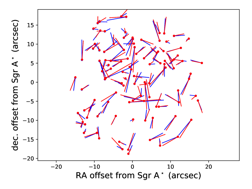
Figure 1: Comparison of proper motion measurements near the Galactic centre. Dots plot the positions of every 5th star brighter than $K=14$ within 19 arcsec of Sgr A from the sample of Fritz et al. (2016), with red streaklines indicating their proper motions. For comparison, the blue streaklines show the corresponding proper-motion measurements from the Schödel et al. (2009) sample.

2.1 Discrete stellar velocities

There are two large recent catalogues of discrete stellar velocities within 1 pc of Sgr A^⋆. Schödel et al. (2009) report proper motions for a sample of more than 6000 stars within an approximately 40 arcsec-square field of view that includes the Galactic centre. Fritz et al. (2016) provide combined proper motions and/or radial velocities for a sample of over $10^{4}$ stars that extends beyond 80 arcsec in projection, albeit with variable coverage in different regions of the sky. As they have spectra for many of their stars, they have better early-type star rejection than Schödel et al. (2009). We use all 4105 stars from Fritz et al. (2016) that lie within a circle of radius 19 arcsec centred on Sgr A^⋆ as the primary source of kinematic data for our models. This circle just touches the boundary of their “extended field” sample. We treat the Schödel et al. (2009) proper motion sample – restricted to the same radius and rescaled to our assumed distance $D=8.3\,\hbox{kpc}$ – as an independent catalogue of the same area. This secondary catalogue has 5005 stars.

Figure 1 shows a comparison of these two catalogues, constructed as follows. From our primary, 19”-radius Fritz et al. (2016) sample we extract all stars brighter than $K=14$. For each such star, we look for matches from the Schödel et al. (2009) sample that lie within a 0.2 arcsec-square box centred on the star and take the one that has the closest match in proper motion. The rms discrepancy in the on-sky components of velocity between the two matched samples is 25 km/s, which is at least a factor four larger than the mean quoted uncertainty in either sample. The cause of this discrepancy is unclear. We note that Fritz et al. (2016) quote a median uncertainty of 8 km/s in their measurements of the line-of-sight components of velocity, which, being obtained from spectra, are unlikely to be affected by whatever causes the discrepancy in the proper motion-derived components. Nevertheless, as a crude method of dealing with the discrepancy we simply set a floor of 20 km/s when modelling the uncertainty of any component of velocity in either sample.

2.2 Outliers and contaminants

Fritz et al. (2016) estimate that as many as 4% of the stars beyond 2 arcsec in their sample could be early type. There are also some stars with anomalously high velocities. We make no attempt to identify and exclude these stars, but instead allow for them in our modelling procedure (Section 3.4 below).

$r_{\rm min}$	$r_{\rm max}$	count	RMS l.o.s. vel.
(arcsec)	(arcsec)		(km/s)
30	40	1362	75
40	50	1487	75
50	60	1580	75
60	70	1652	75
70	80	1710	75
80	100	3555	75
100	120	3692	75
120	150	5726	75
150	200	9889	75
200	250	10184	75
250	300	10391	75
300	500	42824	75

Table 1: Adopted zeroth- and second-order moment profiles binned into circular annuli beyond 1 pc from the cluster centre.

2.3 Profile beyond 19”

Most of the stars in our discrete sample are on orbits that, in three dimensions, take them well beyond the 0.76 pc radius implied by our 19” radius cut. Having some estimate of the outer profile of the cluster helps constrain the orbits of these more loosely bound stars. We take the Nuker-law profile fit by Chatzopoulos et al. (2015), scaled to match the number of stars in our primary sample between 15 and 17 arcsec, and use that to predict star counts within the circular annuli listed in Table 1. Based on the results presented in Feldmeier et al. (2014) and Fritz et al. (2016) we assume that the rms line-of-sight velocity of the stars within each annulus is 75 km/s. In Section 4.1 below we show that the masses fit by our models are only very weakly dependent on the details of the profiles adopted in Table 1; these profiles serve more as a weak prior on the orbit distributions fit by the models.

3 Modelling procedure

We would like to learn what constraints these data place on the cluster’s mass and orbit distribution. The observed stellar catalogue is taken to be a sample drawn from the cluster’s underlying DF. A flexible way of representing the orbit distribution is by expanding this DF as

$$f({\bf x},{\bf v})=\sum_{k=1}^{K}f_{k}e_{k}({\bf x},{\bf v}),$$ (1)

in which $e_{k}({\bf x},{\bf v})$ are basis functions and $f_{k}$ are weights that will be constrained by the data. By Jean’s theorem the $e_{k}$ should be functions only of the integrals of motion ${\bf J}$ in the assumed potential. Because the DF should be non-negative everywhere these $e_{k}$ are often chosen to be non-negative functions with compact support (e.g., Merritt, 1993; Kuijken, 1995; Pichon & Thiebaut, 1998; Wu & Tremaine, 2006). A particularly common choice is to take $e_{k}=\delta({\bf J}-{\bf J}_{k})$ for some set of representative orbits ${\bf J}_{k}$ (e.g., Schwarzschild, 1979; McMillan & Binney, 2012): this is the basis for so-called “Schwarzschild” models. The basis we adopt for this paper is given in Section 3.2 below. Sections 3.3 to 3.5 explain how we calculate the observables for each of our basis elements. Sections 3.6 and 3.7 describe how we fit the coefficients $f_{k}$.

The stars are treated as tracer particles that move in the potential generated by an underlying mass distribution that we would like to constrain. Therefore we do not assume that the mass density profile is proportional to the tracer number density profile: the two are treated independently.

3.1 Coordinate system and potential

We use a coordinate system whose origin $O$ is at the BH. The $z$ axis is parallel to the Galactic rotation axis and the $x$ axis points towards the sun. The $y$ axis then points in the direction of decreasing Galactic longitude $l$ as viewed from the sun. We assume that the cluster has a spherically symmetric mass distribution, with a BH of mass $M_{\bullet}$ at $r=0$, surrounded by a cluster with some specified mass-density profile $\rho(r)$. For example, in our most basic models we take a mass density of the form (Dehnen, 1993; Tremaine et al., 1994)

$$\rho(r)\propto r^{-\gamma}\left(1+\frac{r}{r_{\rm s}}\right)^{-4+\gamma},$$ (2)

with scale radius $r_{\rm s}=10\,\hbox{pc}$, which is well beyond the region where the discrete kinematics are available. The latter extend to $\sim 1\,\hbox{pc}$, which sets a convenient scale at which to normalise the cluster mass. Our simplest mass models then have three free parameters: the black hole mass, $M_{\bullet}$, the extended mass $M_{\star}$ enclosed within 1 pc, and the power-law slope $\gamma$ of its inner density distribution.

3.2 Distribution function

Although we assume that the potential is spherical, we allow the distribution of stars to be axisymmetric about the $Oz$ axis. We ignore variations in stellar populations and assume that the the stellar number density is a function $f({\bf x},{\bf v})$ only of the stars’ phase-space coordinates. By Jeans’ theorem this distribution function (hereafter DF) can depend only on the binding energy ${\cal E}$ per unit mass, the total angular momentum $L$ per unit mass and its component $L_{z}$ projected along the $z$ axis. We divide $({\cal E},L^{2},L_{z})$ space into $K$ blocks and parametrize the DF as

$$f({\cal E},L^{2},L_{z})=\sum_{k=1}^{K}f_{k}{\mathbbm{1}}_{V_{k}}({\cal E},L^{2},L_{z}),$$ (3)

where $V_{k}$ is the physically accessible volume of $({\cal E},L^{2},L_{z})$ space enclosed by the $k^{\rm th}$ block and the indicator function ${\mathbbm{1}}_{V}({\bf w})=1$ if ${\bf w}\in V$ and is zero otherwise. That is, the DF takes on the constant value $f_{k}$ within the $k^{\rm th}$ block. Apart from the constraint that the DF must be non-negative, the parameters $f_{k}\geq 0$ are allowed to vary freely.

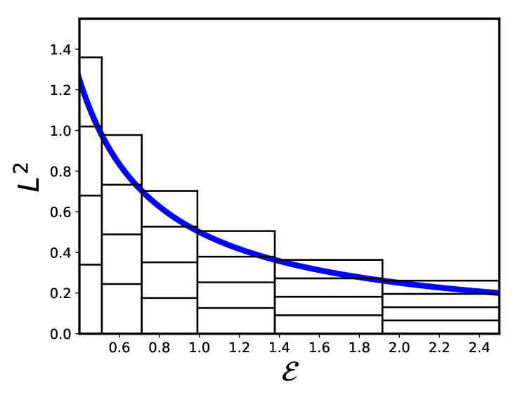
Figure 2: Lindblad diagram illustrating the arrangement of the blocks used to represent the cluster DF $f({\cal E},L^{2})$ for the case $n_{\cal E}\times n_{L^{2}}=6\times 4$. Valid orbits have $L^{2}<L^{2}_{\rm c}({\cal E})$ (heavy solid curve). The $n_{L}$ blocks in a given range of ${\cal E}$ are equispaced in $L^{2}$ with maximum L chosen to just include the boundary of physically allowed orbits.

Figure 2 shows an example of how these $K$ blocks are chosen. We split $({\cal E},L^{2},L_{z})$ integral space into a grid of $K=n_{\cal E}\times n_{L^{2}}\times n_{L_{z}}$ (usually either $200\times 10\times 1$ or $200\times 10\times 8$) abutting rectangular blocks in the following way. First we first select a range of energies ${\cal E}_{0}$,…,${\cal E}_{n_{\cal E}}$ to cover by choosing ${\cal E}_{i}=-\Phi(r_{i})$, where the “apocentre” radii $r_{i}$ are spaced logarithmically between $r_{0}=0.008\,\hbox{pc}$ (about 0.2 arcsec) and $r_{n_{\cal E}}=200\,\hbox{pc}$. The latter is much larger than any of the projected radii for which we have data (Section 2), but we find that such extensive sampling is essential when considering models with extended mass distributions, such as those in Section 5 below. Then for each $({\cal E}_{i},{\cal E}_{i+1})$ the vertical ($L^{2}$) co-ordinates of the block edges are equispaced between 0 and $L_{\rm c}^{2}({\cal E}_{i+1})$, where $L_{\rm c}({\cal E})$ is the angular momentum of a circular orbit of energy ${\cal E}$. This scheme ensures that any orbit whose energy lies between ${\cal E}_{0}$ and ${\cal E}_{n_{\cal E}}$ is included within one of the blocks. The $L_{z}$ boundaries (not shown in Figure 2) are spaced linearly between $L_{z}=-L$ and $L_{z}=+L$, which allows the models to have a net sense of rotation about the $z$ axis. A complete axisymmetric dynamical model then has 16003 parameters: the three parameters $(M_{\bullet},M_{\star},\gamma)$ specifying the potential, plus the parameters $f_{1},\ldots,f_{16000}$ describing the DF.

Expressions for the number density distribution $\nu(R,z)$ and higher-order velocity moments of each orbit block are straightforward to calculate by hand, but tedious to write out. From these we can easily use numerical quadrature to calculate the corresponding projected moments.

3.3 Projected DF and discrete likelihoods

We assume that the discrete kinematical dataset is a fair sample of the cluster’s DF, modulated by a selection function $S({\bf w})$, which gives the probability that a star at phase-space location ${\bf w}=({\bf x},{\bf v})$ would be included in the sample. For all of the examples we consider in this paper, this $S$ will depend only on the star’s $(y,z)$ coordinates. In most cases we adopt the simplest possible model for $S$, a step function that returns 1 when the star’s projected radius, $\sqrt{y^{2}+z^{2}}$, is less than 19 arcsec, and 0 otherwise. This is a drastic simplification, which relies on an assumption that all of the observed stars are approximately at the same distance and that there are no spatial variations in stellar populations. We explore different choices of the selection function in Section 5, including one that models the effects of dust extinction.

The likelihood of observing a star at phase-space position ${\bf w}=({\bf x},{\bf v})$ is then simply

$$\operatorname{pr}({\bf w}|f,\Phi,S)=\frac{1}{I}{\int{\rm d}{\bf w}^{\prime}\,S({\bf w}^{\prime})\operatorname{pr}({\bf w}|{\bf w}^{\prime})f({\bf w}^{\prime}|\Phi)}{},$$ (4)

in which $\operatorname{pr}({\bf w}|{\bf w}^{\prime})$ is the probability that a star having true phase-space coordinates ${\bf w}^{\prime}=({\bf x}^{\prime},{\bf v}^{\prime})$ is observed to be at ${\bf w}=({\bf x},{\bf v})$, $f({\bf w}^{\prime}|\Phi)$ is the orbit-block DF (3) and the denominator

$$I=\int{\rm d}{\bf w}\int{\rm d}{\bf w}^{\prime}\,S({\bf w}^{\prime})\operatorname{pr}({\bf w}|{\bf w}^{\prime})f({\bf w}^{\prime}|\Phi)$$ (5)

ensures that the resulting pdf is correctly normalised. We ignore perspective effects and assume that the on-sky coordinates $(y,z)$ of each star are known perfectly and that every observed star lies somewhere in the range $|x|<x_{\rm max}=200\,\hbox{pc}$ along the line of sight. We assume that each measured component of velocity $v_{l}$ (with $l=x,y,z$) follows an independently distributed normal distribution with dispersion $\Delta v_{l}$ equal to the quoted uncertainty or 20 km/s, whichever is larger (§2). That is, we take

$$\begin{split}&\operatorname{pr}({\bf w}|{\bf w}^{\prime})=\delta(y-y^{\prime})\delta(z-z^{\prime})\operatorname{pr}({\bf v}|{\bf v}^{\prime}),\end{split}$$ (6)

with

$$\begin{split}&\operatorname{pr}({\bf v}|{\bf v}^{\prime})=\\ &\quad\prod_{l=x,y,z}\begin{cases}\frac{1}{\sqrt{2\pi}\Delta v_{l}}\exp\left[-\frac{(v_{l}-v^{\prime}_{l})^{2}}{2\Delta v_{l}^{2}}\right],&\hbox{if $v_{l}$ measured},\\ 1,&\hbox{otherwise}.\end{cases}\end{split}$$ (7)

The likelihood of the discrete kinematical dataset $D$ is then

$$\operatorname{pr}(D|f,\Phi)=\prod_{n=1}^{N}\frac{\sum_{k=1}^{K}P_{nk}f_{k}}{\sum_{k=1}^{K}I_{k}f_{k}},$$ (8)

where

$$P_{nk}=\int_{V_{k}}{\rm d}{\bf w}^{\prime}_{n}\,S({\bf w}_{n}^{\prime})\operatorname{pr}({\bf w}_{n}|{\bf w}^{\prime}_{n},\Phi)$$ (9)

is the probability that a star drawn from the $k^{\rm th}$ orbit block would yield the observed ${\bf w}_{n}=({\bf x}_{n},{\bf v}_{n})$, and the common normalising factor

$$I_{k}=\int{\rm d}{\bf w}\int_{V_{k}}{\rm d}{\bf w}^{\prime}\,S({\bf w}^{\prime}u)\operatorname{pr}({\bf w}|{\bf w}^{\prime},\Phi)$$ (10)

is the probability that a star drawn at random from that block would be included in the discrete catalogue.

In this work we consider selection functions $S=S({\bf x})$ that depend only on the stars’ positions. Then $I_{k}$ is easy to calculate from the three-dimensional density profile of each block. The matrix elements $P_{nk}$ are more involved. For each star $n$ we calculate $P_{n1},...,P_{nK}$ using the following Monte Carlo procedure. We begin by setting $P_{n1}=\cdots=P_{nK}=0$. Then we draw $N_{\rm sample}=10^{5}$ samples of the star’s unknown true velocity ${\bf v}^{\prime}$ from a sampling density

$$\begin{split}f_{\rm s}({\bf v}^{\prime})&=\operatorname{pr}({\bf v}_{n}|{\bf v}^{\prime},\Phi)\\ &\times\prod_{l=x,y,z}\begin{cases}1,&\hbox{if $v_{l}$ measured},\\ {\cal U}(v_{l}^{\prime}|-v_{\rm max},v_{\rm max}),&\hbox{otherwise},\end{cases}\end{split}$$ (11)

where the uniform pdf ${\cal U}(x|a,b)=\frac{1}{b-a}$ if $a<x<b$ and is zero otherwise. We follow McMillan & Binney (2013) in using the same random seed to draw the measured components of each ${\bf v}^{\prime}$ for each trial potential: this reduces noise (but not bias) in the resulting $P_{nk}$ as the potential is varied. The extent of the sampling distribution in the unmeasured components of velocity is set by a conservative bound on the maximum velocity that the star could possibly have in the assumed potential, namely $v_{\rm max}^{2}=-2\Phi(x^{\prime}=0,y^{\prime},z^{\prime})$. Having $(y^{\prime},z^{\prime},v^{\prime}_{x},v^{\prime}_{y},v^{\prime}_{z})$ each position $x^{\prime}$ along the line of sight belongs to a single DF cell $k$. We then walk along $x^{\prime}$, identifying the values of $x$ that mark boundaries between DF cells. For each cell $k$ that we encounter on this walk we increment the corresponding $P_{nk}$ by $\operatorname{pr}({\bf v}_{n}|{\bf v}^{\prime},\Phi)\Delta x^{\prime}/N_{\rm sample}f_{s}({\bf v}^{\prime})$, where $\Delta x^{\prime}$ is the $x^{\prime}$-extent of the cell.

3.4 Interlopers and misidentified stars

Our machinery is designed to model the kinematics of the old stellar population at the Galactic centre. Both Schödel et al. (2009) and Fritz et al. (2016) point out that their catalogues are contaminated by stars from the less relaxed young population. Given the inconsistencies between the two catalogues identified in Section 2 it is also conceivable that some stars could be misidentified when measuring their proper motions.

We account for these possibilities in a simplistic way, replacing $P_{nk}$ by

$$(1-f_{\rm c})P_{nk}+f_{\rm c}P_{nk}^{\infty},$$ (12)

where $f_{\rm c}$ is a contamination fraction and $P_{nk}^{\infty}$ is the probability that a star drawn from block $k$ would be observed at on-sky position $(y_{n},z_{n})$ without any constraints on its velocity. That is, we assume that every star’s measured on-sky position is perfectly correct and consistent with the assumed $S({\bf w})$, but we allow for the possibility that its measured velocity is competely bogus.

Strictly speaking, this is not a true model for interlopers because it assumes that every star included in the catalogue is bound and belongs to the old population. Nevertheless, one might expect that the very general form of the DF in our models means that they have plenty of freedom to “fit around” any small additional bumps in the projected $(y,z)$ number-count distribution caused by genuine interlopers, but that attempting to fit the velocities of such stars would lead to devastating biases on the fitted potential.

3.5 Binned projected zeroth and second moments

These discrete kinematics are supplemented by information on the number counts of stars $c_{b}$ within spatial bins $b=1,...,B$ and the associated rms line-of-sight velocity moments $\sigma^{2}_{b}\equiv\langle v_{x}^{2}\rangle_{b}$. For example, in the application to the Galactic centre dataset, the binned kinematics probe projected radii $R>19^{\prime\prime}$ (e.g., Table 1), beyond the radius where discrete kinematics are used. More generally, we assume that the stars in the discrete dataset and within each spatial bin are independent (i.e., no double counting of stars) and that each bin contains enough stars that we may approximate the underlying Poisson distributions by normal distributions. Then the likelihood (8) gains an extra factor to account for the binned data, becoming (dropping an uninteresting normalisation constant)

$$\begin{split}\operatorname{pr}(D|f,\Phi,S)&=\left[\prod_{n=1}^{N}\frac{\sum_{k}P_{nk}f_{k}}{\sum_{k}I_{k}f_{k}}\right]\exp\left[-\frac{1}{2}\chi^{2}\right],\end{split}$$ (13)

in which $\chi^{2}=\chi_{0}^{2}+\chi_{2}^{2}$ has contributions

$$\begin{split}\chi^{2}_{0}&=\sum_{b=1}^{B}\left(\frac{c_{b}-\sum_{k}Q^{(0)}_{bk}f_{k}}{\sqrt{c_{b}}}\right)^{2}\\ \chi^{2}_{2}&=\sum_{b=1}^{B}\left(\frac{c_{b}\sigma_{b}^{2}-\sum_{b}Q^{(2)}_{bk}f_{k}}{\sqrt{2c_{b}}\sigma^{2}}\right)^{2},\end{split}$$ (14)

from the zeroth- and second-order binned moments, respectively. Here the matrix $Q^{(0)}_{bk}$ is the probability that a star drawn from block $k$ is found in bin $b$. Its elements are calculated by first writing down the (straightforward but tedious) expression for the number-density profile $\nu_{k}(r)$ of orbit block $k$ and then integrating numerically along the lines of sight encompassed by bin $b$. Similarly, $Q^{(2)}_{bk}$ is the $k^{\rm th}$ orbit block’s contribution to the number-weighted second moment integrated over the $b^{\rm th}$ bin and is calculated by numerically integrating the analytical expression for the second-moment distribution $\nu\overline{v_{x}^{2}}({\bf r})$ of the $k^{\rm th}$ orbit block.

In the absence of selection effects (i.e., when all $I_{k}=1$) the expression (13) reduces to that used by Chanamé et al. (2008).

3.6 Anisotropic and isotropic spherical models

Our models assume a spherically symmetric potential $\Phi(r)$, but when $n_{L_{z}}>1$ they have the freedom to fit rotating, axisymmetric DFs $f({\cal E},L^{2},L_{z})$ in this potential. We can enforce spherical symmetry on the DF by merging the $n_{L_{z}}$ orbit blocks for each ${\cal E}$ and $L^{2}$ to produce a DF that is flat in $L_{z}$: having computed the $P_{nk}$, $Q^{(0)}_{nk}$, $Q^{(2)}_{nk}$ and $I_{k}$ projection matrices for an axisymmetric model, we can construct the projection matrices for the corresponding spherical model simply by adding up the $n_{L_{z}}$ elements corresponding to each $({\cal E},L^{2})$ block. Similarly, the matrices for spherical isotropic models are obtained by summing the $n_{L^{2}}\times n_{L_{z}}$ elements for each block in ${\cal E}$.

3.7 Finding the best-fit model

We follow the usual procedure (Rix et al., 1997) of reporting the likelihood of the best-fit non-negative DF for each assumed mass distribution: for each potential we find the vector of DF values $(f_{1},...,f_{K})$ that maximises the likelihood (13), subject only to the constraint that the DF is everywhere non-negative. That is, we assign

$$\operatorname{pr}(D|\Phi,S)\equiv\max_{\{f_{k}\geq 0\}}\operatorname{pr}(D|f,\Phi,S).$$ (15)

To enforce the non-negativity $\{f_{k}\geq 0\}$ constraint we follow Chanamé et al. (2008) in writing $f_{k}=x_{k}^{2}/V_{k}$ then using a conjugate gradient method to find the set $\{x_{k}\}$ that maximises the likelihood (13). We start from an initial guess of $x_{k}^{2}=1/K$, which assigns the same probability mass $f_{k}V_{k}=1/K$ to all orbit blocks.

3.8 Computational costs

For the models presented in this paper the dominant expense in constructing and fitting a single model for an assumed potential $\Phi$ is the calculation of the $P_{nk}$ matrix elements (Section 3.3). It takes about 5 CPU seconds per star to calculate the contribution of all $K$ orbit blocks from $10^{5}$ samples of the star’s velocity. The next biggest expense is typically the calculation of the normalisation coefficients $I_{k}$ (equation 10). If $S({\bf w})$ varies over an orbit then this requires numerical integration; the integral over velocities can be carried out analytically, but the integration over the spatial coordinates must be carried out numerically.

The likelihood maximisation requires a few thousand iterations to converge for our spherical anisotropic models with $n_{{\cal E}}\times n_{L^{2}}\times n_{L_{z}}=200\times 10\times 1$ orbit blocks. This takes about a minute for our test models with 1000 stars (Section 4 below) to about 10 minutes for our models of the real Galaxy with $4105$ stars (Section 5). Axisymmetric models with $n_{{\cal E}}\times n_{L^{2}}\times n_{L_{z}}=200\times 10\times 8$ take significantly longer to converge.

    all 3 components of ${\bf v}$ proper motions only line-of-sight only

spherical isotropic

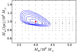
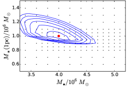
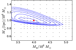
spherical anisotropic

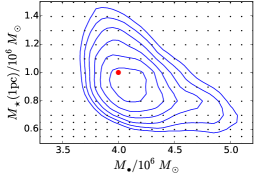
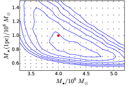
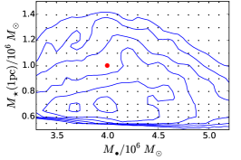
axisymmetric

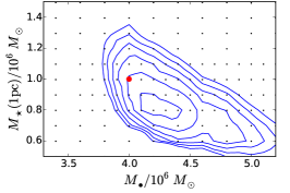
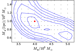
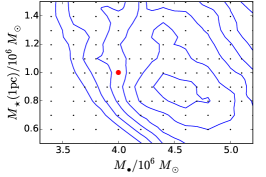
Figure 3: Likelihoods $\operatorname{pr}(D_{0}|M_{\bullet},M_{\star},S)$ of models fit to data $D_{0}$ of the simulated cluster described in Section 4. These models assume the correct form for the stellar potential, leaving only the black hole mass $M_{\bullet}$ and cluster mass $M_{\star}$ as free parameters. From top to bottom the panels show results for spherical isotropic, spherical anisotropic and axisymmetric models. The left column shows results for the case in which all three components of velocity are available for the inner discrete data. The middle and right columns show results when only proper motions and line-of-sight velocities, respectively, are available. Successive contours are spaced by $\Delta\log\operatorname{pr}(D_{0}|M_{\bullet},M_{\star},S)=1$, with the innermost contour starting at $0.5$ below the peak value of $\log\operatorname{pr}(D_{0}|M_{\bullet},M_{\star},S)$; this innermost contour would then indicate the “1-sigma” uncertainty on $M_{\bullet}$ or $M_{\star}$ if the likelihood were perfectly Gaussian. In each panel the red dot indicates the correct value of the parameters $(M_{\bullet},M_{\star})$. The fainter black dots show the locations at which the log likelihoods have been calculated to construct the contours.

4 Tests with mock observations of simulated clusters

Before applying our modelling machinery to the real Galactic centre we first test it against mock data drawn from a variety of simple model clusters. The density profiles of these simulated clusters vary, but each has a central BH of mass $4\times 10\,M_{\odot}$ and an extended mass of $M_{\star}=10^{6}\,M_{\odot}$ enclosed within $1\,\hbox{pc}$.

To generate the simulated data for each cluster we solve for the cluster’s DF and from that draw a large number of stellar positions and velocities, scattering each component of velocity by a random number drawn from a normal distribution with standard deviation equal to the assumed observational uncertainty of $20\,\hbox{km/s}$. The mock observations consist of a discrete sample of $10^{3}$ such stars that lie within a projected radius of 19” of the BH, plus stellar number counts and second-order line-of-sight velocity moments summed over the on-sky annuli given in Table 1.

4.1 A spherically symmetric cluster

Our first simulated cluster is spherically symmetric. Its mass- and number-density profiles are given by eq. (2) with a scale radius $r_{\rm s}=10\,\hbox{pc}$ and inner slope $\gamma=1$ (Hernquist, 1990). The cluster has an isotropic velocity distribution. To construct our simulated catalogue we use the standard Eddington inversion procedure (e.g., Binney & Tremaine, 2008) to find its DF $f({\cal E})$ and then draw stellar positions and velocities from that.

4.1.1 Recovery of $M_{\bullet}$ and $M_{\star}$ assuming the correct (unnormalised) density profile

The most basic test of the modelling procedure outlined in §3 is whether it can recover the parameters of the mass distribution when the correct underlying functional form (2) is assumed. This profile has four free parameters: $M_{\bullet}$, $M_{\star}$, $\gamma$ and $r_{\rm s}$. A full scan over all four would be prohibitively expensive. So, we start by constructing models that assume the correct shape ($\gamma=1$) and radial scale ($r_{\rm s}=10\,\hbox{pc}$) for the mock cluster, leaving only the pair of mass normalisation parameters $(M_{\bullet},M_{\star})$ to be constrained.

For each $(M_{\bullet},M_{\star})$ pair we calculate the potential and set up a grid of $K=n_{\cal E}\times n_{L^{2}}\times n_{L_{z}}=200\times 10\times 8$ orbit blocks with apocentre radii spaced logarithmically between $0.008\,\hbox{pc}\simeq 0.02^{\prime\prime}$ and $200\,\hbox{pc}$. Then we calculate the $P_{nk}$ matrix for the 1000 discrete stars, the $Q^{(0)}_{bk}$ and $Q^{(2)}_{bk}$ matrices for the binned moments, and the normalisation factors $I_{k}$ assuming the selection function $S$ equals 1 inside projected radius $R>19^{\prime\prime}$ and zero outside. Having calculated these matrices we use the maximization procedure of §3.7 to find the likelihood $\operatorname{pr}(D|\Phi,S)$. To fit spherical anisotropic or isotropic model to the data we can merge these axisymmetric DF blocks as described in §3.6 before carrying out the likelihood maximization.

Figure 3 shows the resulting likelihoods, $\operatorname{pr}(D|M_{\bullet},M_{\star},S)$, under various assumptions about the underlying galaxy model. From top to bottom, the rows show the results for spherical isotropic models ($n_{L^{2}}=n_{L_{z}}=1$), spherical anisotropic models ($n_{L^{2}}=10$, $n_{L_{z}}=1$) and axisymmetric $f(E,L^{2},L_{z})$ models ($n_{L^{2}}=10$, $n_{L_{z}}=8)$. The left-most column shows models that fit all three components of each discrete velocity. The middle column shows fits to proper motions only (i.e., the $P_{nk}$ matrix is recalculated assuming complete ignorance of the line-of-sight component of velocity), while the rightmost column shows the result of fitting only to the line-of-sight component, ignoring proper motions.

In all but one case the correct $(M_{\bullet},M_{\star})=(4,1)\times 10^{6}\,M_{\odot}$ is well within the 95% credible interval returned by the models (assuming a flat prior on either $M_{\bullet}$ and $M_{\star}$ or on their logarithms). The spherical isotropic models provide particularly tight constraints on $(M_{\bullet},M_{\star})$. This is not surprising, because such models have no freedom in their internal dynamics once their radial mass- and number-density profiles are given. The number-density distribution is not completely determined by the discrete observations, however. Therefore, the greater the number of components of velocity used for the discrete stellar sample, the tighter the constraints on the mass parameters from the isotropic models become.

The spherical anisotropic models have much more freedom, as is evident from the widening of their likelihood contours compared to the isotropic ones. Again, the tightest constraints are obtained when all three components of velocity are available. The axisymmetric models have yet more freedom. On closer inspection of the spherical anisotropic and axisymmetric models we find that the $\chi^{2}$ of the fit to the binned outer data (equation 14) is typically very small, varying between about 0.1 and 2 (for the 24 datapoints implied by Table 1), provided $M_{\star}>0.5\times 10^{6}\,M_{\odot}$. Nevertheless, these binned outer profiles are essential for ruling out the most outlandish orbit distributions: the likelihood contours of models fit only to the discrete inner stellar data are much noisier, showing that without the constraints provided by the outer binned data the anisotropic models are freer to overfit the details of the discrete stellar distribution. There is an extremely steep increase in $\chi^{2}$ as $M_{\star}$ falls below the threshold value of $0.5\times 10^{6}\,M_{\odot}$. This is the cause of the sharp cutoff in the bottom edge of the contours plotted in Figure 3.

We note that the best-fitting $M_{\bullet}$ in the anisotropic and axisymmetric models shown in Figure 3 tends to be an overprediction of the true value. There is a corresponding underprediction of $M_{\star}$, consistent with the characteristic mass estimate of the combined BH+cluster system being better constrained than either $M_{\bullet}$ or $M_{\star}$ individually. As a quick check of the significance of these systematically high best-fit $M_{\bullet}$ values we have generated a number of further discrete realisations of the cluster model and fit axisymmetric models to those. In some cases the resulting best-fit values of $M_{\bullet}$ are higher than the true one, while in other cases they are lower. So, although we are unable to prove formally that our implementation of the DF-superposition method produces unbiased estimates of $M_{\bullet}$ and $M_{\star}$, the results plotted in Figure 3 do not constitute evidence for such a bias.

    all 3 components of ${\bf v}$ proper motions only line-of-sight only

spherical isotropic

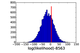
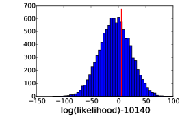
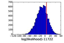
spherical anisotropic

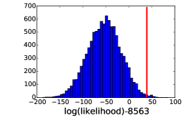
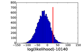
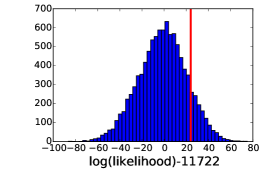
axisymmetric

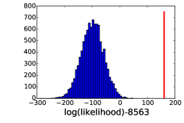
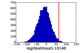
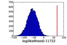
Figure 4: Log likelihoods of various realisations of the models shown in Figure 3. In each panel the zero point of the horizontal axis indicates the log likelihood $\log\operatorname{pr}(D_{0}|f,\Phi,S)$ of the initial dataset $D_{0}$ drawn from the simulated cluster’s underlying smooth DF $f$. The heavy vertical red line indicates the log-likelihood $\log\operatorname{pr}(D_{0}|f_{0},\Phi,S)$ of the DF-superpostion model $f_{0}$ that best fits these data. Notice that this $\log\operatorname{pr}(D_{0}|f_{0},\Phi,S)$ is always at least as large as $\log\operatorname{pr}(D_{0}|f,\Phi,S)$ and becomes larger as $f_{0}$ becomes more flexible (top to bottom rows). The histograms plot the distribution of log likelihoods $\log\operatorname{pr}(D_{i}|f_{0},\Phi,S)$ of an ensemble of datasets $D_{1}$, $D_{2}$, …, each of 1000 stars drawn from this best-fit DF $f_{0}$.

4.1.2 Testing for overfitting

When DF-superposition models are fit to integrated stellar kinematics the likelihood becomes a Gaussian, $\operatorname{pr}(D|{\bf f},\phi)\propto\exp[-\frac{1}{2}\chi^{2}]$, in which $\chi^{2}[{\bf f}]$ is some quadratic form in the orbit weights $(f_{1},...,f_{K})$. Valluri et al. (2004) have pointed out that the usual “maximum-likelihood” procedure for considering only the very best-fitting orbit weights ${\bf f}$ for each potential leads anomalously low values of $\chi^{2}$: the models overfit the data. We have just seen that our models tend to produce fits to binned, outer data that are too good to be true, with $\chi^{2}<2$. Magorrian (2006) provided an explanation for such behaviour, starting from the observation that this $\chi^{2}$ is a hugely degenerate quadratic form in the orbit weights. He argued that the the correct resolution of the overfitting problem was to marginalise ${\bf f}$ after adopting a suitable prior, but nevertheless found that in an example problem the standard “maximum-likelihood” procedure does produce reliable BH masses, albeit with formal uncertainties on $M_{\bullet}$ which are slightly too tight. The situation with discrete kinematical data is less clear, however, because the likelihood (8) is not a Gaussian. In the following we carry out some simple checks to test for overfitting in the discrete case.

Let $D_{0}$ be the “observed” discrete stellar kinematics of our simulated cluster, and let $f$ the the smooth underlying DF from which these are drawn. When we feed this $D_{0}$ into our DF-superposition modelling code, it produces some best-fit DF, represented as a weighted sum of orbit blocks. We call this fitted DF $f_{0}$. Assuming the correct potential $\Phi$ is used, we expect the likelihood $\operatorname{pr}(D_{0}|f_{0},\Phi)$ of this fitted model to be larger than or equal to the likelihood $\operatorname{pr}(D_{0}|f,\Phi)$ of the “true” model $f$, because the block DF $f_{0}$ has sufficient flexibility to fit the details of the “observed” data $D_{0}$, while including (an approximate, discretized version of) the true $f$ as a special case.

Figure 4 shows that this is indeed the case. The heavy vertical red line in each panel indicates the log likelihood $\log\operatorname{pr}(D_{0}|f_{0},\Phi,S)$ of the best-fit model for each of the cases considered in Figure 3. The log-likelihoods of the best-fit spherical, isotropic models (left column) are within $\sim 1$ of the log-likelihoods of the smooth models $f$ from which the data were generated. The best-fit spherical anisotropic models have $\log\operatorname{pr}(D_{0}|f_{0},\Phi,S)$ larger than $\log\operatorname{pr}(D_{0}|f,\Phi,S)$, the difference becoming even larger for more general axisymmetric models.

From each of these best-fit models $f_{0}$ we draw further discrete realisations $D_{1}$, $D_{2}$, …., each of 1000 stars subject to the selection function $S$. A minimal sanity check of the fit $f_{0}$ is then whether the (log) likelihood of the original dataset, $\log\operatorname{pr}(D_{0}|f_{0},\Phi,S)$, is typical in the sense that it lies among the (log) likelihoods $\{\log\operatorname{pr}(D_{n}|f_{0},\Phi,S)\}$ of these resampled datasets (see also Binney & Wong (2017), who carry out a similar test for the models of the MW’s globular cluster system). The distribution of these log likelihoods is plotted as the histograms in each panel of Figure 4. By the central limit theorem each distribution is approximately Gaussian: the log-likelihood is a sum of 1000 terms, all drawn from the same projected PDF. For our samples of 1000 stars, the dispersion of this Gaussian ranges from about 20 for models fit only to line-of-sight components of velocity up to around 50 for models fit to all three components. It is clear that the spherical isotropic models pass this test, whereas axisymmetric models do not: for the latter $\operatorname{pr}(D_{n}|f_{0},\Phi,S)\ll\operatorname{pr}(D_{0}|f_{0},\Phi,S)$, demonstrating that the fit $f_{0}$ to $D_{0}$ is very special indeed in these cases.

Although we do not plot them here, the log likelihoods of samples $D_{n}$ drawn from the original smooth DF $f$ have approximately the same variance as those drawn from $f_{0}$, but have means close to the log likelihood $\log\operatorname{pr}(D_{0}|f,\Phi,S)$ of our original sample. Therefore, for the simulated observational setup we consider here, a condition that is broadly equivalent to the $\chi^{2}\simeq N\pm\sqrt{2N}$ plausibility criterion for integrated stellar kinematics is that $\log\operatorname{pr}(D|f,\Phi,S)\simeq\log\operatorname{pr}(D_{0}|f_{0},\Phi,S)\pm\Delta\sqrt{N/1000}$, where $\Delta\simeq 20$ for models that fit only the line-of-sight components of velocity, up to $\Delta\simeq 50$ for models fit to all three components. Our spherical isotropic models pass this test. Spherical anisotropic models do show a tendency to overfit, but much less so than the axisymmetric models. In the remainder of this paper we focus on fitting only spherical anisotropic models.

4.1.3 Degeneracies in the DF

This overfitting is a symptom of the decision to consider only a single, very special best-fit DF $f_{0}$ for each potential $\Phi$. This $f_{0}$ achieves its remarkably good fit by itself becoming implausibly noisy. One way of dealing with this (e.g., Valluri et al., 2004, and references therein) is by penalising nonsmooth DFs by maximising a penalized likelihood $\log\operatorname{pr}(D|{\bf f},\Phi)+\lambda P[{\bf f}]$, in which a penalty function $P$ is introduced to quantify some measure of “smoothness” of the DF $f$. The weight $\lambda$ given to the penalty function might be chosen by using experiments such as those in Section 4.1.2 above to ensure that the favoured model’s likelihood is within a plausible range of values. This is sensible if one wants to pick out a single representative DF for the assumed potential and believes that the smoothness conditions imposed by the penalty function are reasonable.

This is less satisfactory if one wants to compare different potentials or does not want to exclude DFs with sharp features. An alternative solution (e.g., Magorrian, 2006) is to note that, although the “best” $f_{0}$ fits the data implausibly well, there will be vastly more “nearby” DFs that produce fits that are formally slightly worse, but with likelihood values that are in fact more plausible. The natural remedy is somehow to take account of these neighbouring DFs. In the present case in which we approximate the DF as a discrete sum of orbit blocks this could be achieved by marginalising the weights $f_{k}$, but carrying out such a calculation is beyond the scope of this paper.

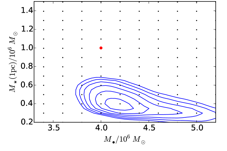
Figure 5: Likelihoods of spherical anisotropic models fit to data comprising all three components of velocity from our simulated cluster assuming a mass density (2) with the correct slope $\gamma=1$ but with a scale radius $r_{\rm s}=100\,\hbox{pc}$ that is a factor of 10 too large. Fitting only the proper motions produces similar results.

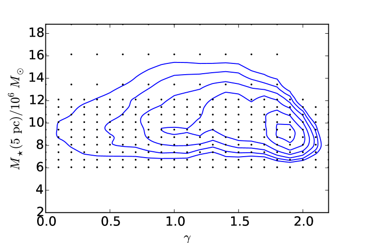
Figure 6: Dependence of log-likelihood of on $\gamma$ and $M_{\star}(5\hbox{pc})$ for models fit to all three components of velocity in our simulated dataset. The models use the correct value of $M_{\bullet}$, but assume a scale radius $r_{\rm s}=100\,\hbox{pc}$ that is a factor 10 too large.

4.1.4 How well is the radial mass profile constrained?

We have just seen that our modelling machinery can successfully constrain the mass normalisation $M_{\star}$ of the stellar cluster, provided the functional form and scale radius of the mass density profile were somehow known in advance. To investigate how well the models behave in more realistic situations we begin by fitting models that adopt the correct $\gamma=1$ for the mass-density slope, but take the scale radius of the mass distribution to be $r_{\rm s}=100\,\hbox{pc}$ instead of the correct 10 pc.

The resulting likelihood contours are plotted in Figure 5. They show that the models predict the correct black hole mass, but underestimate the extended mass enclosed within 1 pc by a factor of at least 2. Our motivation for choosing this $1\,\hbox{pc}$ reference radius was that it is approximately equal to the maximum projected radius of the discrete kinematics ($R=19^{\prime\prime}\simeq 0.74\,\hbox{pc}$), but the Figure demonstrates that this is actually a very poor choice. It turns out that it is much better to choose a reference radius that accounts for the three-dimensional distribution of the sampled stars. The selection function for our discrete stellar sample defines a very long, narrow cylinder of radius 19” whose axis includes the observer and the BH at the centre of the cluster. The RMS three-dimensional radius of stars within this cylinder is approximately $5\,\hbox{pc}$: in three dimensions the stellar sample is strongly elongated along the line of sight. The $r_{\rm s}=10\,\hbox{pc}$ simulated cluster from which we drew the kinematics has an extended mass of $13.4\times 10^{6}\,M_{\odot}$ within this $5\,\hbox{pc}$.

Figure 6 shows the effects on the likelihood of varying the density slope $\gamma$ in a model that assumes the correct $M_{\bullet}$, but takes $r_{\rm s}=100\,\hbox{pc}$, a factor $10$ too large. Although the overall peak occurs for $\gamma\sim 1.8$ – presumably because that squeezes more mass close to the BH – the best-fitting models all have $M_{\star}(5\hbox{pc})\sim 10\times 10^{6}\,M_{\odot}$. This is systematically lower than the true $M_{\star}(5\,\hbox{pc})=13.4\times 10^{6}\,M_{\odot}$, but significantly less biased than the models’ estimate of $M_{\star}(1\,\hbox{pc})$ and, remarkably, almost independent of $\gamma$. The log likelihood of this best-fitting $\gamma=1.8$ model is only 0.5 less than that of the model that uses the correct mass distribution. This is perhaps not surprising given the limited radial extent of the discrete data we use. Changing the reference radius much from $5\,\hbox{pc}$ increases the bias on the mass estimate and breaks the independence from $\gamma$.

    all 3 components of ${\bf v}$ proper motions only line-of-sight only

40 disc stars

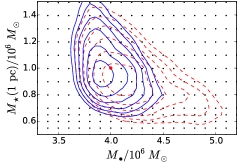
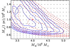
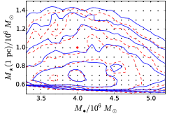
100 disc stars

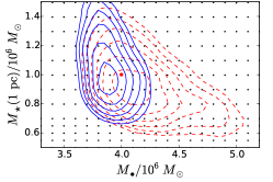
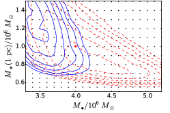
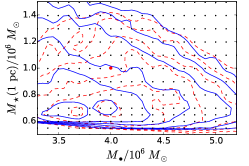
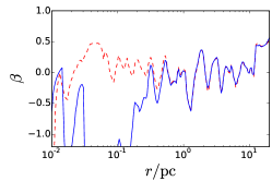
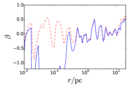
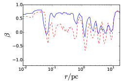
Figure 7: As for Figure 3, but illustrating the effects of a nonspherical contaminant population on the masses returned by spherical, anisotropic models. The top row shows the result of adding 40 stars from the tilted ring distribution described in the text, the middle row the result of adding 100. For reference, the dashed red contours plot the likelihoods (repeated from the middle row of Figure 3) of models fit to the uncontaminated spherical population. The bottom panel compares the anisotropy parameters of models that assume that correct potential, but are fit to the uncontaminated sample (dashed red curves) versus those contaminated by 100 disc stars (solid blue curves).

4.2 Nonspherical clusters

All of our tests so far have involved fitting spherical and axisymmetric models to simulated observations of spherical clusters. Having shown that our axisymmetric models tend to overfit the data, we have confined our attention to spherical models. Now we investigate how well these spherical models perform when applied to simulated observations of nonspherical clusters.

4.2.1 Effects of a tilted ring of young stars

Although the old population of our Galaxy’s stellar cluster is roughly spherical in its inner parsec or so, there is a substantial population of young stars distributed in a ring-like structure in the innermost few tenths of a parsec. Ideally one would like to remove any such young stars from the sample, but that relies on spectroscopic identification, which is not always available. To investigate the effects of such nonspherical contaminants, we adopt a very simple model of the Milky Way’s young star population based on the fits in Paumard et al. (2006) and Yelda et al. (2014). Our model is a razor-thin ring of stars moving on circular orbits with radii $1^{\prime\prime}<r<13^{\prime\prime}$. Their face-on number density distribution goes as $r^{-2}$. Referred to our $(x,y,z)$ coordinate system (§3.1) the disc’s normal vector is taken to be ${\bf n}=(-\cos I,\sin I\cos\Omega,-\sin I\sin\Omega)$ with $(I,\Omega)=(130^{\circ},96^{\circ})$. We add stars from this tilted ring population to the sample of 1000 stars drawn from the simulated spherical cluster introduced in §4.1. There is no change to the potential of the simulated cluster: the ring stars are treated as massless test particles.

As in §4.1.1 we test our DF-superposition modelling procedure by giving it the correct form for the radial mass profile, leaving only the mass normalisation parameters $M_{\bullet}$ and $M_{\star}(1\hbox{pc})$ as parameters to be determined. Figure 7 plots the likelihood as functions of these two parameters for spherical anisotropic models fit to all three components of velocity of the population of 1000 “old” stars used for Figure 3, to which we have added a further 40 (4% contamination fraction, top row) or 100 (very high 10% contamination fraction, bottom row) stars from the “young” tilted ring population. We note first that the models that fit only to line-of-sight velocities are largely unaffected by this contamination: they are just as wrong afterwards as they were before. The models that use proper motion information are more interesting: increasing the fraction of disc contaminants biases the inferred orbit distribution towards tangential orbits ($\beta<0$) for $r\lesssim 13^{\prime\prime}$, which in turn depresses the estimate of $M_{\bullet}$. This depression is less pronounced when all three components of velocity are available.

We have investigated whether our simple model for outliers (§3.4) can correct this bias, but find that setting $f_{\rm c}>0$ just depresses the estimate of $M_{\bullet}$ further. This failure is not too suprising though: the outlier model is intended to account for stars whose velocities are simply mismeasured, not significant populations of stars that break the underlying symmetry assumption.

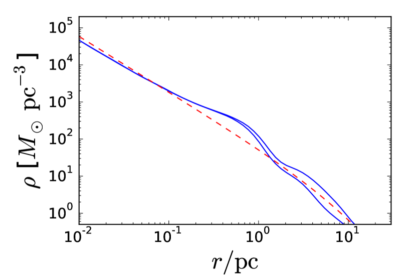
Figure 8: Density profiles of the flattened simulated cluster introduced in §4.2.2. The blue curves plot the cluster’s major- and minor-axis mass density profiles. For comparison, the dashed curve shows the form (18) of the mass density profile assumed by our spherical anisotropic DF-superposition models.

4.2.2 Fitting spherical models to a simulated flattened cluster

Although the Milky Way’s central star cluster is approximately round in projection for projected radii $R<1\,\hbox{pc}$, it does become flattened further out. Most of the stars that lie within the $R<19^{\prime\prime}\simeq 0.74\,\hbox{pc}$ cylinder we use to sample the discrete kinematics have three-dimensional radii $r\gg 1\,\hbox{pc}$, placing many of them in the region where the cluster starts to become strongly flattened. To test to what extent this is likely to bias the masses returned by our models we consider kinematics from a simulated flattened cluster.

Our starting point for constructing this simulated cluster is the multi-Gaussian fit to the Milky Way’s NIR projected light distribution between 10 and 2500 arcsec made by Schödel et al. (2014, their Table 4). At smaller radii their multi-Gaussian parametrization introduces a central core of almost constant density. To produce a more realistic, cusped density profile we add to this a further component having surface brightness

$$I(R)=I_{0}\left(\frac{R}{R_{0}}\right)^{-0.5}\left(1+\frac{R}{R_{0}}\right)^{-3.5},$$ (16)

with $R_{0}=20^{\prime\prime}$ and $I_{0}=10^{7}\,L_{\odot,4.5\,\mu{\rm m}}/\hbox{pc}^{2}$. We deproject the resulting surface brightness distribution under the assumption that the cluster is axisymmetric and viewed edge on. We assume that mass follows light and normalise the resulting $\rho(R,z)$ mass density so that the stellar mass enclosed within a spherical radius of $1\,\hbox{pc}$ is $10^{6}\,M_{\odot}$. Figure 8 plots the major- and minor-axis mass density profiles of the deprojected cluster. The $\nu(R,z)$ number-density profile of our simulated cluster is directly proportional to this $\rho(R,z)$.

    all 3 components of ${\bf v}$ proper motions only line-of-sight only

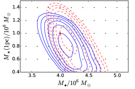
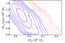
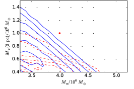
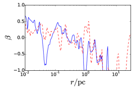
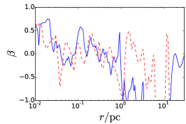
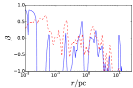
Figure 9: Top row: likelihood contours (blue curves) of spherical anisotropic models fit to the kinematics of the simulated flattened cluster described in §4.2.2. For comparison, the dashed red contours show likelihoods of spherical models fit to the corresponding simulated spherical clusters. The red dot indicates the correct $(M_{\bullet},M_{\star})=(4,1)\times 10^{6}\,M_{\odot}$. Bottom row: anisotropy profiles of the best-fitting models that assume this correct potential.

We use a multipole expansion to calculate the stellar contribution to the potential, and add a central BH of mass $M_{\bullet}=4\times 10^{6}\,M_{\odot}$. Our simulated cluster has a two-integral DF $f({\cal E},L_{z})$, the even-in-$L_{z}$ part of which, $f_{+}$, is completely determined by the known $\nu(R,z)$ and $\Phi(R,z)$ through

$$\nu(R,z)=\frac{4\pi}{R}\int_{0}^{\psi(R,z)}\,{\rm d}{\cal E}\int_{0}^{\sqrt{2R^{2}(\psi(R,z)-{\cal E})}}{\rm d}L_{z}\,f_{+}({\cal E},L_{z}).$$ (17)

We ignore the odd-in-$L_{z}$ part of the DF because the nonrotating spherical models that we will use to fit the simulated kinematics are blind to it. Our procedure for inverting (17) to find $f_{+}$ borrows the same techniques we use to construct our DF-superposition models: we represent the DF $f_{+}({\cal E},L_{z})$ as a sum of blocks (3) in $({\cal E},L_{z})$, calculate the contribution that each block makes to the densities $\nu(R,z)$ at a set of points in the $(R,z)$ plane and then find the set of block weights that best reproduces the deprojected $\nu(R,z)$. Having found $f_{+}$ we draw stellar positions and velocities from it. Our simulated discrete catalogue then consists of 1000 stars having projected radius $R<19^{\prime\prime}$ drawn from this $f_{+}$ and scattered by $20\hbox{km\,s}^{-1}$ simulated observational uncertainty. We also calculate the zeroth- and second-order velocity moments of $f_{+}$ averaged over the annuli given in Table 1.

For comparison purposes, we also construct a spherical, isotropic reference cluster that matches the density and potential of the flattened cluster along its symmetry axis. That is, the DF $f({\cal E})$ of this spherical cluster is set equal to $f_{+}({\cal E},L_{z}=0)$ and samples of stars drawn from it to construct simulated catalogues in the same way as the axisymmetric models.

We use the modelling procedure of Section 3 to fit spherical anisotropic models to the simulated kinematics from both axisymmetric and spherical clusters. Although it would be possible to take, say, the deprojected minor-axis profile plotted in Figure 8 for the DF-superposition models’ $\rho(r)$ profile, we have opted for convenience to take

$$\rho(r)\propto r^{-1.5}\left(1+\frac{r}{r_{\rm s}}\right)^{-1.5},$$ (18)

with $r_{\rm s}=10\,\hbox{pc}$ instead. This was obtained using a crude “by-eye” fit to the deprojected $\rho(0,z)$ profile.

Figure 9 shows how the likelihoods of the models varies with the assumed $(M_{\bullet},M_{\star})$ for this $\rho(r)$. Models that fit only the line-of-sight components of velocity do not reproduce the correct potential or orbit distribution. For the other two cases it is clear that any systematic error in the inferred masses caused by fitting these spherical models to the data from this flattened simulated cluster is no larger than that induced by a smattering of “young” stars on tilted ring orbits. Internally, the main systematic difference caused by the neglect of flattening is a slight bias towards tangential orbits at radii $r>1\,\hbox{pc}$; the effect on the inferred masses is small.

    (a) Omit inner 2” (b) Omit inner 8” (c) Dust (d) Schödel+2009 sample

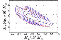
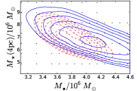
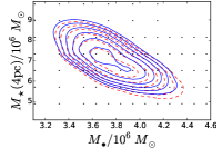
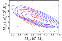
Figure 10: Likelihoods of models fit to real data, assuming mass density of the form (2) with an inner power-law slope $\gamma=1.5$ and a scale radius $r=300\,\hbox{pc}$. For reference, the dashed red contours in each panel show the likelihoods of models fit to the stellar kinematics of Fritz et al. (2016) within $R=19^{\prime\prime}$; these contours are the same in all four panels. From left to right, the blue contours show models that: (a) fit only to stars having $2^{\prime\prime}<R<19^{\prime\prime}$; (b) fit only to stars that have $8^{\prime\prime}<R<19^{\prime\prime}$; (c) use all stars having $R<19^{\prime\prime}$, but modifying the selection function to account for a simple two-dimenstional exintinction model; (d) fit to the $R<19^{\prime\prime}$ subset of the Schödel et al. (2009) catalogue instead of Fritz et al. (2016).

5 Application to the Galactic centre

Having investigated some of the most obvious potential sources of systematic error introduced by our implementation of the DF-superposition procedure with the spherical symmetry assumption, we now apply it to the real Galactic centre.

5.1 Power-law mass density profiles

An important feature of our models is that we do not assume that the cluster’s unknown mass density profile is directly related to the number-density distribution of the stars used as kinematical tracers. Both observations (Schödel et al., 2018) and theoretical arguments (Baumgardt et al., 2018) suggest that the underlying mass density of the Milky Way’s nuclear cluster is approximately a power law, $\rho\sim r^{-\gamma}$, with $\gamma\simeq 1.5$, at least in the innermost parsec or so. Our first models adopt a mass density of the form (2) with $r_{\rm s}=300\,\hbox{pc}$ and $\gamma=1.5$, so that the assumed $\rho(r)$ is very close to this pure power law over the volume of space probed by the observed stars. That leaves the BH mass $M_{\bullet}$ and the normalisation $M_{\star}$ of the surrounding extended mass distribution as the free parameters in our potential. For comparison with the results of Chatzopoulos et al. (2015) we use $4\hbox{pc}\simeq 100^{\prime\prime}$ as the reference radius for calculating $M_{\star}$.

The dashed red contours in each panel of Figure 10 show the likelihood contours of $(M_{\bullet},M_{\star})$ obtained by fitting the kinematics of all 4105 of the stars from Fritz et al. (2016) that have $R<19^{\prime\prime}$ together with the binned zeroth- and second-order moments from Table 1. The best-fit $M_{\bullet}=(3.88\pm 0.21)\times 10^{6}\,M_{\odot}$ and $M_{\star}(4\,\hbox{pc})=(6.76\pm 0.54)\times 10^{6}\,M_{\odot}$, only slightly lower than the measurements of $4.0\times 10^{6}\,M_{\odot}$ to $4.3\times 10^{6}\,M_{\odot}$ obtained from the S stars (Boehle et al., 2016; Gillessen et al., 2017).

We now show that our result is independent of these S stars. We can excise the “central field” ($R<2^{\prime\prime}$) of the Fritz et al. (2016) sample by setting the selection function $S(y,z)$ to zero outside the range $2^{\prime\prime}<R<19^{\prime\prime}$, recalculating the likelihood normalisations $I_{k}$ (equation 10) and refitting the models ignoring the 59 stars from the innermost 2”. Doing this has almost no effect on $(M_{\bullet},M_{\star})$ (blue contours on left-most panel of Figure 10).

A more striking result is obtained by dropping the 793 stars that have $R<8^{\prime\prime}$, within which most of the population of young stars live. Omitting this region results in a significant increase in the BH mass estimate to $M_{\bullet}=(4.08\pm 0.32)\times 10^{6}\,M_{\odot}$ (second panel of Figure), but leaves $M_{\star}(4\,\hbox{pc})=(6.75\pm 0.75)\times 10^{6}\,M_{\odot}$ almost unchanged.

We can also use the selection function to test the effects of dust extinction. Schödel et al. (2010) have used stellar $H-K_{\rm s}$ colours to construct an two-dimensional extinction map of the Galactic centre region: given a position $(y,z)$, they provide an estimate of the $K_{\rm s}$-band extinction to the Galactic centre along that line of sight. Following their Figure 9 we assume that the luminosity function of the stars that comprise the kinematical catalogue scales as $L(m)\propto 10^{0.27m}$, where $m$ is the star’s absolute $K_{\rm s}$-band luminosity. Then the probability that a star is bright enough to be included in the catalogue scales as $S(y,z)\propto 10^{-0.27A_{K}(y,z)}$. The results of fitting models in which the normalisation integrals $I_{k}$ have been adjusted to use this selection function are shown on the third panel of Figure 10. This suggests that our results are unlikely to be strongly affected by extinction.

There are a couple of caveats associated with this reassuring result, however. The first is that the Schödel et al. (2010) exinction map is available for a slightly offset rectangular region that covers most, but not all, of the 19”-radius cylinder that defines our kinematical sample: for lines of sight $(y,z)$ that are unavailable in their map we assume that the extinction is equal to the average of the available $A_{K}$ values that have the same projected radius. The second is that this dust model assumes that the extinction is caused by a two-dimensional screen of dust that lies between us and the Galactic centre: it ignores any variation in the dust density along lines of sight within the Galactic centre region. Chatzopoulos et al. (2015) show how such variations can be constrained by looking for asymmetries in velocity histograms, but note that they are not likely to strongly affect the even-in-$L_{z}$ part of their $f({\cal E},L_{z})$ DF (which is effectively what our nonrotating spherical anisotropic models use).

Our models produce similar results when fit to the independently obtained proper catalogue of Schödel et al. (2009): the rightmost panel of Figure 10 plots the $(M_{\bullet},M_{\star})$ likelihood contours obtained by fitting all 5005 stars within $R=19^{\prime\prime}$ from this sample. The best-fit $M_{\bullet}=(3.98\pm 0.52)\times 10^{6}\,M_{\odot}$ with $M_{\star}(4\,\hbox{pc})=(6.62\pm 0.98)\times 10^{6}\,M_{\odot}$. Even though we have adjusted the quoted uncertainties on both kinematical datasets (Section 2) to be consistent with each other, it is nevertheless reassuring that the two datasets produce comparable mass estimates.

    (a) $\gamma=1.5$ (b) Chatzopoulos+2015 (c) $\gamma=1.5$ extended

   

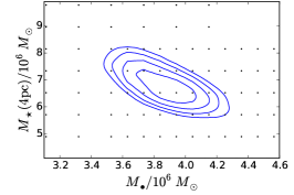
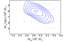
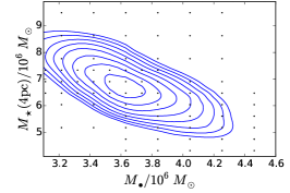
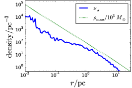
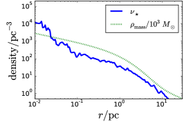
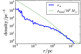
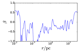
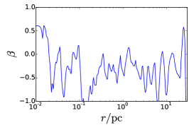
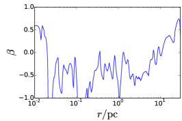
Figure 11: A comparison of different mass models fit to the Fritz et al. (2016) kinematics. From left to right, the columns show: (a) the reference model from Figure 10, which has a mass density profile of the form (2) with $\gamma=1.5$ and $r_{\rm s}=300\,\hbox{pc}$; (b) models that adopt the form of the mass density profile used by Chatzopoulos et al. (2015); (c) models having mass-density profile (19). The top panel in each column shows how the model’s likelihoods depend on the assumed $(M_{\bullet},M_{\star})$. The same contours levels are used in all three columns: the more contours shown, the more likely the model. The middle panel that shows the mass-density profile of the best-fitting model (dotted curves), together with the inferred number density profile (solid curve). The lower panel plots the best-fit model’s anisotropy profile.

Our models make no assumptions about the underlying number density or anisotropy of the stars, apart from spherical symmetry. The first column of Figure 11 shows the number-density and anisotropy profiles for our $\gamma=1.5$, $r_{\rm s}=300\,\hbox{pc}$ fit to the $R<19^{\prime\prime}$ subset of the Fritz et al. (2016) sample in more detail. Notice that this number density profile becomes shallower within about $1\,\hbox{pc}$, only to steepen again inside $0.1\,\hbox{pc}$. In this model there is a significant “unseen” mass component within about 1 parsec of the centre that is not sampled by the observed kinematical tracers. The model is broadly isotropic, except for a bias towards circular orbits for $0.1<r/\hbox{pc}<0.2$ (approximately 2.5” to 5”) and is consistent with expectations from our simulated clusters (Figure 7).

At radii $r<0.02\,\hbox{pc}$ (approximately 0.5”) the model becomes radially biased, with $\beta=0.5$. The Fritz et al. (2016) sample contains only 7 stars having projected radius $R<0.5^{\prime\prime}$. Therefore we do not attach any significance to the $\beta(r)$ profile at these small radii.

5.2 More realistic mass-density profiles

Chatzopoulos et al. (2015) construct their spherical and axisymmetric isotropic models assuming that number and mass densities are both of the form

$$\begin{split}\rho(r)&=\frac{(3-\gamma)M_{1}}{4\pi}\frac{r_{\rm s}}{r^{\gamma}(r+r_{\rm s})^{4-\gamma}}\\ &\quad+\frac{(3-\gamma_{2})M_{2}}{4\pi}\frac{r_{\rm s,2}}{r^{\gamma_{2}}(r+r_{\rm s,2})^{4-\gamma_{2}}},\end{split}$$ (19)

which includes an additional component of mass $M_{2}$ added to the profile (2). They fit this profile to the projected number density profile measured by Fritz et al. (2016), obtaining best-fit parameters $\gamma=0.51$, $r_{\rm s}=99^{\prime\prime}$, $\gamma_{2}=0.07$, $r_{\rm s,2}=2376^{\prime\prime}$ and mass ratio $M_{2}/M_{1}=105.45$ when they assume spherical symmetry. Notice that the inner scale radius $r_{\rm s}=99^{\prime\prime}\simeq 4\,\hbox{pc}$ is much smaller than the $r_{\rm s}=300\,\hbox{pc}$ we use for the models we have just considered. The second column of Figure 11 shows our spherical anisotropic models fit assuming this mass profile. In these models the assumed underlying mass-density profile is a closer fit to the number-density profile of the kinematical tracers. The BH mass returned by the models is $M_{\bullet}=(3.91\pm 0.20)\times 10^{6}\,M_{\odot}$, which is in good agreement with the $M_{\bullet}=(3.86\pm 0.14)\times 10^{6}\,M_{\odot}$ produced by the isotropic axisymmetric models of Chatzopoulos et al. (2015). Our $M_{\star}$ lies between the $M_{\star}(4\hbox{pc})=(8.94\pm 0.31)\times 10^{6}\,M_{\odot}$ they found using their axisymmetric isotropic models and the $M_{\star}(4\hbox{pc})\simeq 5\times 10^{6}\,M_{\odot}$ from their spherical isotropic models.

Our best-fitting model with this mass density profile has a log likelihood that is 1.1 higher than the best-fitting $\rho\sim r^{-1.5}$ model shown in the left column of the Figure. Both assumed forms for the mass distribution yield similar anisotropy profiles and best-fit values of $M_{\bullet}$, with only the best-fit value of $M_{\star}(4\,\hbox{pc})$ changing slightly between the two.

We can produce yet better fits to the data by tweaking the parameters used in the mass density (19). For example, the right-most column of Figure 11 shows models that have $M_{2}/M_{1}=300$ and $\gamma=1.5$, but keep all other parameters the same those used by Chatzopoulos et al. (2015). The “unseen” mass fraction in the innermost parsec is higher even than the first models and the BH mass is reduced to $M_{\bullet}=(3.62\pm 0.20)\times 10^{6}\,M_{\odot}$ with $M_{\star}(4\,\hbox{pc})=(6.77\pm 0.54)\times 10^{6}\,M_{\odot}$. This has a log likelihood that is 3.6 larger than our best $\rho\sim r^{-1.5}$, $M_{2}=0$ model plotted in the left-most column. Again, the anisotropy profile is largely unchanged in the innermost few parsecs.

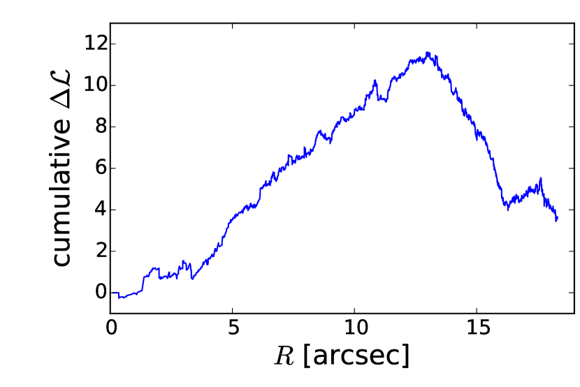
Figure 12: Cumulative change in the log-likelihood $\Delta{\cal L}_{n}=\log\operatorname{pr}(D_{n}|\Phi_{2})-\log\operatorname{pr}(D_{n}|\Phi_{1})$ of individual stars $n=1,...,4105$ ordered by their projected radius $R_{n}$. Here $\Phi_{1}$ is the potential of the almost pure “power-law” $\rho\sim r^{-1.5}$ mass model used in the left panel of Figure 10, while $\Phi_{2}$ is the more realistic potential implied by (19) shown in the right panel of the same figure. In both cases $M_{\bullet}=3.7\times 10^{6}\,M_{\odot}$ and $M_{\star}(4\hbox{pc})=6.2\times 10^{6}\,M_{\odot}$.

An immediate question is whether it is possible to identify the cause of this increase of 3.6 in the log likelihood between the two $\gamma=1.5$ models. We have examined the change in the log likelihoods of individual stars for models with $(M_{\bullet},M_{\star})=(3.7,6.2)\times 10^{6}\,M_{\odot}$ when one replaces the almost-pure $r_{\rm s}=300\,\hbox{pc}$ power-law cusp (2) (left column of Figure 11) with the varying slope on superparsec scales implied by the density profile (19) (right column of same Figure). Figure 12 shows that breaking the pure power-law in the density tends to improve the likelihoods of stars between about 4 and 13 arcsec, albeit at the cost of those outside that. This suggests that it might be possible to “tune” the form of the mass density by examining how the likelihoods of individual stars are affected as the assumed mass profile changes. We do not pursue it further in this paper, however, because we expect that the systematic errors induced in the likelihoods by our neglect of flattening are likely to be comparable in size.

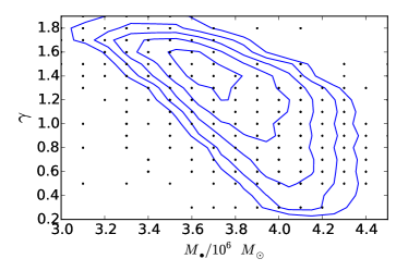
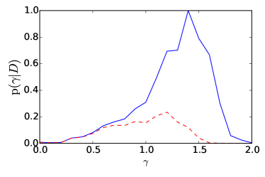
Figure 13: Constraints on the inner power-law slope, $\gamma$, of the mass density profile (19) with $M_{2}/M_{1}=300$ and all other parameters equal to those used by Chatzopoulos et al. (2015). The panel on the left shows the posterior distribution of $(\gamma,M_{\bullet})$ obtained by marginalizing $M_{\star}$ assuming flat priors on $\gamma$, $M_{\bullet}$ and $M_{\star}$. The panel on the right shows the result of a further marginalization of $M_{\bullet}$ if all $M_{\bullet}$ are allowed (solid curve) or with the restriction that $M_{\bullet}>4\times 10^{6}\,M_{\odot}$ (dashed curve).

Figure 13 shows the effect of different choices of the assumed inner power-law slope $\gamma$ of the mass density (19) with $M_{2}/M_{1}=300$. Marginalising $\gamma$, the constraints on the BH mass are $M_{\bullet}=(3.76\pm 0.22)\times 10^{6}\,M_{\odot}$. Conversely, marginalising $M_{\bullet}$, the formal constraints on $\gamma$ are $\gamma=1.3\pm 0.3$, although this would drop to $\gamma=1.0\pm 0.3$ if we were to insist that $M_{\bullet}>4\times 10^{6}\,M_{\odot}$.

6 Conclusions

Although the mass of the BH at the Galactic centre is now reasonably well constrained, much less is known about the structure of surrounding stellar cluster. The motivation for this paper was to find out what can be established about the mass and orbit distribution of this cluster by using DF-superposition models to fit positions and velocities of stellar catalogues (Schödel et al., 2009; Fritz et al., 2016) that probe the central few parsecs. Our models assume spherical symmetry, but otherwise make no assumption about the cluster’s internal anisotropy or its radial number-count distribution: the observed stellar catalogues are treated as a (projected) sample of the cluster’s underlying DF, subject to a known selection function $S({\bf w})$.

6.1 Constraints on BH mass

The mass $M_{\bullet}$ of the central BH sets an important boundary condition that any dynamical model of the Galactic centre should match. We have carried out extensive tests with data from simulated clusters to probe how well our models reproduce this constraint. Although the models tend to overfit the data, they nevetheless do reproduce the correct $M_{\bullet}$ provided the simulated cluster is spherical. Fitting spherical models to simulated clusters in which this symmetry has been broken (e.g., by introducing a tilted ring of stars or by flattening the cluster at larger radii) results in estimates of $M_{\bullet}$ that are biased 5–10% low.

When applied to the kinematical dataset of Fritz et al. (2016) our models produce a BH of mass $M_{\bullet}=(3.76\pm 0.22)\times 10^{6}\,M_{\odot}$, very similar to the value found by Chatzopoulos et al. (2015) using isotropic axisymmetric Jeans models on the same data, but slightly lower than the values obtained by directly fitting the orbits of the S stars (Boehle et al., 2016; Gillessen et al., 2017). Our best-fitting models are broadly isotropic, but they do show a bias towards circular orbits at radii where the young stellar disc is strongest. Omitting all stars at such radii from our fitting procedure pushes our estimate of $M_{\bullet}$ up to values that are comfortably within the range favoured by the analyses based on the S stars (Figure 10).

Although we have not mentioned it explicitly yet, an even more important source of systematic error on $M_{\bullet}$ is the assumed distance $D$ to the Galactic centre. In the absence of any line-of-sight velocity constraints, the mass estimates produced by our models scale as $(D/8.3\,\hbox{kpc})^{3}$: a 5% error in $D$ produces a 15% error in $M_{\bullet}$. This is unlikely to be a significant contributor to the origin of the small discrepancy between our models and the the S-star analyses though, because fundamentally the latter have the same $M_{\bullet}\propto D^{3}$ dependence (in the absence of any line-of-sight velocity constraints).

6.2 Constraints on the distribution of matter around the BH

The stars from the “extended field” of Fritz et al. (2016) are largely confined to the BH’s sphere of influence. It is not surprising then that the constraints our models place on the mass distribution around the BH are much weaker than those on the BH mass itself. In particular, we find that proper motions are essential if the models are to provide reliable virial-like characteristic mass estimates of the surrounding cluster: the DF of models that fit only line-of-sight velocities (e.g., Figures 3 and 9) are underconstrained and, lacking any treatment for the degeneracies in the orbit weight distribution, return a biased result.

On the other hand, when proper motions (or, even better, all three components of velocity) are available then the stars do act as useful probes of the extended mass distribution within which they move, even if one has to work hard to place interesting constraints on $\rho(r)$ (Section 4.1.4). For example, our best-fit models of the Galaxy centre have power-law density profiles $\rho\sim r^{-\gamma}$ with $\gamma\simeq 1.3\pm 0.3$ in the inner parsec (Figure 13). That is based on a small sample of plausible $\rho(r)$ parametrizations, but careful scrutiny of how the likelihoods of individual stars change depending on the the assumed potential (Figure 12) may offer a way to tune the form of $\rho(r)$.

We have deliberately restricted our models to stars having $R<19^{\prime\prime}$, all of which lie within the “extended field” of Fritz et al. (2016). Including stars at larger radii would help anchor the form of $\rho(r)$. Indeed, kinematics for such stars already exist in the literature (e.g., in the “large field” and “outer field” regions of Fritz et al. (2016) and in the sample of Feldmeier et al. (2014)). There is nothing fundamentally difficult about modelling stars from many such catalogues simultaneously: the simplest way would be to adjust the selection function $S({\bf w})$ to account for the inevitable variations in the sampling depth of each catalogue. For such an endeavour to be worthwhile, however, we would need to relax our convenient assumption that the potential is spherically symmetric: this is marginally acceptable for stars having $R<19^{\prime\prime}$, but becomes increasingly implausible as one moves beyond the sphere of influence of the BH into the region where the flattened cluster starts to dominate the potential. It remains to be seen by how much the overfitting problem would affect the reliability of results from these more general models applied to more extensive data.

6.3 General

Stepping back, it is remarkable that discrete, likelihood-based schemes can be used to place any interesting constraints on the potential: one is looking for changes in the log likelihood of order unity, with the log likelihood itself being a sum of contributions from thousands of stars; even the slightest bias in the calculation of likelihoods of individual stars will be amplified hugely. As a slightly artificial example of this, consider the treatment of individual stellar velocity measurements. We have assumed that the observed velocity is normally distributed about the star’s true underlying velocity. Our model for interlopers (eq. 12) can be thought of as adding an extended halo to the Gaussian that represents the likelihood of each star. When we include such halos by setting $f_{\rm c}\gtrsim 10^{-6}$ we find that the estimates of $M_{\bullet}$ for both simulated and real data are depressed. The most immediate interpretation is that this interloper model is at best incomplete.

Apart from symmetry, an even more fundamental assumption shared by the vast majority of dynamical mass estimation methods is that the system has relaxed to a steady state. We do not test the consequences of that assumption here, but Kowalczyk et al. (2018) have, albeit in a different context – using orbit-superposition models to fit the kinematics of simulated $N$-body dwarf spheroidal galaxies formed by disc mergers. The machinery for fitting discrete kinematics presented in this paper could also be applied to dwarf spheroidal galaxies, but in many ways the Galactic centre problem is simpler (e.g., the potential is simpler; there are no issues with identifying the location of the centre of the cluster; the effects of contamination by stellar binaries are less likely to be significant).

References

- Baumgardt et al. (2018) Baumgardt H., Amaro-Seoane P., Schödel R., 2018, A&A, 609, A28
- Binney & Tremaine (2008) Binney J., Tremaine S., 2008, Galactic Dynamics: Second Edition
- Binney & Wong (2017) Binney J., Wong L. K., 2017, MNRAS, 467, 2446
- Boehle et al. (2016) Boehle A., Ghez A. M., Schödel R., Meyer L., Yelda S., Albers S., Martinez G. D., Becklin E. E., Do T., Lu J. R., Matthews K., Morris M. R., Sitarski B., Witzel G., 2016, ApJ, 830, 17
- Chakrabarty & Saha (2001) Chakrabarty D., Saha P., 2001, AJ, 122, 232
- Chanamé et al. (2008) Chanamé J., Kleyna J., van der Marel R., 2008, ApJ, 682, 841