On analyzing and evaluating privacy measures for social networks under active attack

Abstract

Widespread usage of complex interconnected social networks such as Facebook, Twitter and LinkedIn in modern internet era has also unfortunately opened the door for privacy violation of users of such networks by malicious entities. In this article we investigate, both theoretically and empirically, privacy violation measures of large networks under active attacks that was recently introduced in (Information Sciences, 328, 403–417, 2016). Our theoretical result indicates that the network manager responsible for prevention of privacy violation must be very careful in designing the network if its topology does not contain a cycle. Our empirical results shed light on privacy violation properties of eight real social networks as well as a large number of synthetic networks generated by both the classical Erdös-Rényi model and the scale-free random networks generated by the Barábasi-Albert preferential-attachment model.

1 Introduction

Due to a significant growth of applications of graph-theoretic methods to the field of social sciences in recent days, it is by now a standard practice to use the concepts and terminologies of network science to those social networks that focus on interconnections between people. However, social networks in general may represent much more than just networks of interconnections between people. Rapid evolution of popular social networks such as Facebook, Twitter and LinkedIn have rendered modern society heavily dependent on such virtual platforms for their day-to-day operation. The powers and implications of social network analysis are indeed indisputable; for example, such analysis may uncover previously unknown knowledge on community-based involvements, media usages and individual engagements. However, all these benefits are not necessarily cost-free since a malicious individual could compromise privacy of users of these social networks for harmful purposes that may result in the disclosure of sensitive data (attributes) that may be linked to its users, such as node degrees, inter-node distances or network connectivity. A natural way to avoid this consists of an “anonymization process” of the relevant social network in question. However, since such anonymization processes may not always succeed, an important research goal is to be able to quantify and measure how much privacy a given social network can achieve. Towards this goal, the recent work in [43] aimed at evaluating the resistance of a social network against active privacy-violating attacks by introducing and studying theoretically a new and meaningful privacy measure for social networks. This privacy measure arises from the concept of the so-called $k$-metric antidimension of graphs that we explain next.

Given a connected simple graph $G=(V,E)$, and an ordered sequence of nodes $S=\left(v_{1},\dots,v_{t}\right)$, the metric representation of a node $u$ that is not in $S$ with respect to $S$ is the vector (of $t$ components) $\mathbf{d}_{u,-S}=(\mathrm{dist}_{u,v_{1}},\dots,\mathrm{dist}_{u,v_{t}})$, where $\mathrm{dist}_{u,v}$ represents the length of a shortest path between nodes $u$ and $v$. The set $S$ is then a $k$-antiresolving set if $k$ is the largest positive integer such that for every node $v$ not in $S$ there also exist at least other $k-1$ different nodes $v_{j_{1}},\dots,v_{j_{k-1}}$ not in $S$ such that $v,v_{j_{1}},\dots,v_{j_{k-1}}$ have the same metric representation with respect to $S$ (i.e., $\mathbf{d}_{v,-S}=\mathbf{d}_{v_{j_{1}},-S}=\dots=\mathbf{d}_{v_{j_{k-1}},-S}$). The $k$-metric antidimension of $G$ is defined to be value of the minimum cardinality among all the $k$-antiresolving sets of $G$ [43]. If a set of attacker nodes $S$ represents a $k$-antiresolving set in a graph $G$, then an adversary controlling the nodes in $S$ cannot uniquely re-identify other nodes in the network (based on the metric representation) with probability higher than $\nicefrac{{1}}{{k}}$. However, given that $S$ is unknown, any privacy measure for a social network should quantify over all possible subsets $S$ of nodes. In this sense, a social network ${G}$ meets ${(k,\ell)}$-anonymity with respect to active attacks to its privacy if ${k}$ is the smallest positive integer such that the ${k}$-metric antidimension of ${G}$ is no more than ${\ell}$. In this definition of ${(k,\ell)}$-anonymity the parameter ${k}$ is used for a privacy threshold, while the parameter ${\ell}$ represents an upper bound on the expected number of attacker nodes in the network. Since attacker nodes are in general difficult to inject without being detected, the value $\ell$ could be estimated based on some statistical analysis of other known networks. A simple example that explains the role of $k$ and $\ell$ to readers is as follows. Consider a complete network $K_{n}$ on $n$ nodes in which every node is connected with every other node. It is readily seen that for any $0<\ell<n$, this network meets $(n-\ell,\ell)$-anonymity. In other words, this means that a social network $K_{n}$ guarantees that a user cannot be re-identified (based on the metric representation) with a probability higher than ${1}/({n-\ell})$ by an adversary controlling at most $\ell$ attacker nodes. For other related concepts for metric dimension of graphs, the reader may consult references such as [14, 25, 30].

Chatterjee et al. in [9] (see also [49]) formalized and analyzed the computational complexities of several optimization problems motivated by the ${(k,\ell)}$-anonymity of a network as described in [43]. In this article, we consider three of these optimization problems from [9], namely Problems 1–3 as defined in Section 2. A high-level itemized overview of the contribution of this article is as follows (see Section 3 for precise technical statements and details of all contributions):

1. Our theoretical result concerning the anonymity issues for networks without cycles is provided in Theorem 1 in Section 3.1. Some consequences of this theorem are also discussed immediately following a statement of the theorem.

2. In Section 3.2, we first describe briefly efficient implementations of the high-level algorithms of Chatterjee et al. [9] for Problems 1–3 (namely Algorithms I and II in Section 3.2.1). We then tabulate and discuss the results of applying these implemented algorithms for the following type of network data:

   1. eight real social networks listed in Table 3 in Section 3.4.2,

   2. the classical undirected Erdös-Rényi random networks $G(n,p)$ for four suitable combinations of $n$ and $p$, and

   3. the scale-free random networks $G(n,q)$ generated by the Barábasi-Albert preferential-attachment model for four suitable combinations of $n$ and $q$.

   The ${6}$ tables that provide tabulations of the empirical results are Tables 4–9 in Section 3.2 and the type of conclusions that one can draw from these tables are stated in the ${11}$ conclusions numbered ①– in the same section. Despite our best efforts, we do not know of any other alternate approaches (e.g., sybil attack framework) that will provide a significantly simpler theoretical framework to reach all the ${11}$ conclusions as mentioned above.

As an illustration of a potential application, consider the hub fingerprint query model of Hey et al. [26]. Noting that the largest hub fingerprint for a target node $u$ is the metric representation of $u$ with respect to the hub nodes, results on $(k,\ell)$-anonymity are directly applicable to this setting of Hey et al. [26] that models an adversary trying to identify the hub nodes in a network. For example, assuming that the quantity ${k}_{\mathrm{opt}}$ in Problem 1 (see Section 2 for a definition) is $10$, the network is vulnerable with respect to hub identification in the model of Hey et al. in the sense that it is not possible to guarantee that an adversary will not be able to uniquely re-identify any node in the network with probability at most $0.1$.

1.1 Some remarks regarding the model and our contribution (to avoid possible confusion)

To avoid any possible misgivings or confusions regarding the technical content of the paper as well as to help the reader towards understanding the remaining content of this article, we believe the following comments and explanations may be relevant.

1. The computational complexity investigations in this paper has nothing to do with the model in the paper by Backstrom et al. [5]. We whole-heartedly and without any reservations agree that the paper by Backstrom et al. [5] is seminal, but the research investigations in this paper has nothing to do with the model or any measure introduced in the paper by Backstrom et al. [5]. The notion of active attack is very different in that paper, and therefore the computational problems that arise in that paper are very different from those in the current paper and in fact incomparable. Finally, the goal of this paper is not to compare various network privacy models but to investigate, theoretically and empirically, the model in [43].

2. This paper does not introduce any new privacy model or measure, but simply investigates, both theoretically and empirically, computational problems for a model that is published in “Information Sciences, 328, 403–417, 2016” (reference [43]). There have been several other subsequent papers investigating this privacy measure, e.g., see [9, 44, 49, 34]. Thus, researchers in network privacy are certainly interested in this model or related computational complexity questions. Of course, this does not contradict the fact that the paper by Backstrom et al. [5] is seminal.

3. Even though the network privacy model was introduced in [43] and therefore the best option for clarification of any confusion regarding the model would be to look at that paper, we provide the following clarification just in case. In this model, nobody is trying to prevent adversaries. Informally, the privacy measure only gives a “measure” on how much secure a graph is against active attacks, i.e., a probability with which we can assert that, if there are controlled nodes in a graph, then we can in some sense know which is the probability to be reidentified in such graph (for details please see the texts preceding and following the statements of Problems 1–3 in Section 2). No new nodes are added at all. This is not a problem that involves dynamic graphs. The model in [43] is not the same as the one by Backstrom et al. [5].

1.2 Comparison with other existing works

1.2.0.0.1 Model comparison

Unfortunately, different models of network privacy have quite different objectives and consequently quite different measures that cannot in general be compared to one another. In particular, we know of no other different but comparable model or measure of network privacy that can be compared to those in our paper. For example, the network privacy model introduced by Backstrom et al. [5] is interesting, but the notion of active attack is very different in that paper, and therefore the computational problems that arise in that paper are very different from those in the current paper and in fact incomparable.

1.2.0.0.2 Algorithmic comparison

Note that algorithms for different models cannot be compared in terms of their worst-case (or average-case) computational complexities. For example, consider the scale-free network model and the computational complexity paper for this model in [21]. Now, consider the Erdös-Rényi random regular network model, and consider the paper in [51]. Even though [51] provides better algorithmic results in terms of time-complexity and approximability, that does not nullify the research results in [21].

1.2.0.0.3 Privacy preservation in learning theoretic framework

The recent surge in popularity of machine learning applications to different domains, specifically in the context of deep learning methods, has motivated many Internet companies to provide numerous online cloud-based services and frameworks for developing and deploying machine learning applications (Machine Learning as a Service or MLaaS) such as the Google Cloud ML Engine. Typically, an user (customer) of such a system first estimates the parameters of a suitable model by training the model with data and afterwards, once the correct model is determined, uploads the model to the cloud provider such that remote users can use the model. This type of service frameworks lead to two possible privacy concerns, the first concerning privacy violations of the training data, and the second concerning privacy violations of data uploaded by remote users. For some recent papers dealing with possible remedies of these privacy violations, such as introducing suitable random noises to perturb the data, see papers such as [40, 50]. However, these privacy concerns are quite different from the current topic of our paper, such as they are not specific to networks and they involve learning paradigms which are not of interest to this paper. Whether privacy questions in the MLaaS framework can be combined with those in this paper is an interesting research question but unfortunately beyond the scope of this paper.

2 Basic notations, relevant background and problem formulations

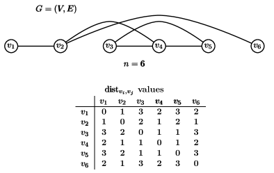
Figure 1: An example for illustration of some basic definitions and notations in Section 2.

Let $G=(V,E)$ be the undirected input network over $n$ nodes $v_{1},\dots,v_{n}$. The authors in [9] formalized and analyzed the computational complexities of several optimization problems motivated by the $(k,\ell)$-anonymity of a network as described in [43]. The notations and terminologies from [9] relevant for this paper are as follows (see Fig 1 for an illustration):

1. $\mathbf{d}_{v_{i}}=\left(\mathrm{dist}_{v_{i},v_{1}},\mathrm{dist}_{v_{i},v_{2}},\dots,\mathrm{dist}_{v_{i},v_{n}}\right)$ denotes the metric representation of a node $v_{i}$. For example, in Fig 1, $\mathbf{d}_{v_{1}}=\left(0,1,3,2,3,2\right)$.

2. $\mathsf{Nbr}\left(v_{\ell}\right)=\left\{\,v_{j}\,|\,\left\{v_{\ell},v_{j}\right\}\in E\,\right\}$ is the (open) neighborhood of node $v_{\ell}$ in $G=(V,E)$. For example, in Fig 1, $\mathsf{Nbr}\left(v_{2}\right)=\left\{\,v_{1},v_{4},v_{6}\,\right\}$.

3. For a subset of nodes $V^{\prime}=\left\{v_{j_{1}},v_{j_{2}},\dots,v_{j_{t}}\right\}\subset V$ with $j_{1}<j_{2}<\dots<j_{t}$ and any other node $v_{i}\in V\setminus V^{\prime}$, $\mathbf{d}_{v_{i},-V^{\prime}}=\big{(}\mathrm{dist}_{v_{i},v_{j_{1}}},\mathrm{dist}_{v_{i},v_{j_{2}}},\dots,\mathrm{dist}_{v_{i},v_{j_{t}}}\big{)}$ denotes the metric representation of $v_{i}$ with respect to $V^{\prime}$. The notation is further generalized by defining $\mathcal{D}_{V^{\prime\prime},-V^{\prime}}=\left\{\,\mathbf{d}_{v_{i},-V^{\prime}}\,|\,v_{i}\in V^{\prime\prime}\,\right\}$ for any $V^{\prime\prime}\subseteq V\setminus V^{\prime}$. For example, in Fig 1, $\mathbf{d}_{v_{3},-\left\{v_{1},v_{5},v_{6}\right\}}=\big{(}\underset{v_{1}}{3},\underset{v_{5}}{1},\underset{v_{6}}{3}\big{)}$ and $\mathcal{D}_{\left\{v_{2},v_{3}\right\},-\left\{v_{1},v_{5},v_{6}\right\}}=\big{\{}(\overbrace{\underset{v_{1}}{1},\underset{v_{5}}{2},\underset{v_{6}}{1}}^{\text{\footnotesize from $v_{2}$}}),(\overbrace{\underset{v_{1}}{3},\underset{v_{5}}{1},\underset{v_{6}}{3}}^{\text{\footnotesize from $v_{3}$}})\big{\}}$.

4. A partition $\Pi^{\prime}=\left\{V_{1}^{\prime},V_{2}^{\prime},\dots,V_{\ell}^{\prime}\right\}$ of $S^{\prime}\subseteq V$ is called a refinement of a partition $\Pi=\left\{V_{1},V_{2},\dots,V_{k}\right\}$ of $S\supseteq S^{\prime}$, denoted by $\Pi^{\prime}\prec_{\mathpzc{r}}\Pi$, provided $\Pi^{\prime}$ can be obtained from $\Pi$ in the following manner:

   1. For every node $v_{i}\in\left(\cup_{t=1}^{k}V_{t}\right)\setminus\left(\cup_{t=1}^{\ell}V^{\prime}_{t}\right)$, remove $v_{i}$ from the set in $\Pi$ that contains it.

   2. Optionally, for every set $V_{\ell}$ in $\Pi$, replace $V_{\ell}$ by a partition of $V_{\ell}$.

   3. Remove empty sets, if any.

   For example, for Fig 1, $\left\{\{v_{2}\},\{v_{3}\},\{v_{4},v_{5}\}\right\}\prec_{\mathpzc{r}}\left\{\{v_{1},v_{2},v_{3}\},\{v_{4},v_{5}\}\right\}$.

5. The following notations pertain to the equality relation (an equivalence relation) over the set of (same length) vectors $\mathcal{D}_{V\setminus V^{\prime},-V^{\prime}}$ for some $\emptyset\subset V^{\prime}\subset V$:

   1. The set of equivalence classes, which forms a partition of $\mathcal{D}_{V\setminus V^{\prime},-V^{\prime}}$, is denoted by $\Pi_{{V\setminus V^{\prime},-V^{\prime}}}^{=}$. For example, in Fig 1, $\mathcal{D}_{\left\{v_{2},v_{3},v_{4},v_{5}\right\},-\left\{v_{1},v_{6}\right\}}=\big{\{}(\overbrace{\underset{v_{1}}{1},\underset{v_{6}}{1}}^{\text{\footnotesize from $v_{2}$}}),(\overbrace{\underset{v_{1}}{3},\underset{v_{6}}{3}}^{\text{\footnotesize from $v_{3}$}}),(\overbrace{\underset{v_{1}}{2},\underset{v_{6}}{2}}^{\text{\footnotesize from $v_{4}$}}),(\overbrace{\underset{v_{1}}{3},\underset{v_{6}}{3}}^{\text{\footnotesize from $v_{5}$}})\big{\}}$ and
      $\Pi_{\left\{v_{2},v_{3},v_{4},v_{5}\right\},-\left\{v_{1},v_{6}\right\}}^{=}=\Big{\{}\,\big{\{}(\overbrace{\underset{v_{1}}{1},\underset{v_{6}}{1}}^{\text{\footnotesize from $v_{2}$}})\big{\}},\big{\{}(\overbrace{\underset{v_{1}}{2},\underset{v_{6}}{2}}^{\text{\footnotesize from $v_{4}$}})\big{\}},\big{\{}(\overbrace{\underset{v_{1}}{3},\underset{v_{6}}{3}}^{\text{\footnotesize from $v_{3}$}}),(\overbrace{\underset{v_{1}}{3},\underset{v_{6}}{3}}^{\text{\footnotesize from $v_{5}$}})\big{\}}\,\Big{\}}$.

   2. Abusing terminologies slightly, two nodes $v_{i},v_{j}\in V\setminus V^{\prime}$ will be said to belong to the same equivalence class if $\mathbf{d}_{v_{i},-V^{\prime}}$ and $\mathbf{d}_{v_{j},-V^{\prime}}$ belong to the same equivalence class in $\Pi_{{V\setminus V^{\prime},-V^{\prime}}}^{=}$, and thus $\Pi_{{V\setminus V^{\prime},-V^{\prime}}}^{=}$ also defines a partition into equivalence classes of $V\setminus V^{\prime}$. For example, in Fig 1, $v_{3}$ and $v_{5}$ belong to the same equivalence class in $\Pi_{\left\{v_{2},v_{3},v_{4},v_{5}\right\},-\left\{v_{1},v_{6}\right\}}^{=}$ and $\Pi_{\left\{v_{2},v_{3},v_{4},v_{5}\right\},-\left\{v_{1},v_{6}\right\}}^{=}$ also defines the partition $\big{\{}\{v_{2}\},\{v_{4}\},\{v_{3},v_{5}\}\big{\}}$.

   3. The measure of the equivalence relation is defined as $\mu\left(\mathcal{D}_{V\setminus V^{\prime},-V^{\prime}}\right)\stackrel{{\scriptstyle\mathrm{def}}}{{=}}\min_{\mathcal{Y}\in\Pi_{{V\setminus V^{\prime},-V^{\prime}}}^{=}}\big{\{}\,\left|\,\mathcal{Y}\,\,\right|\big{\}}$. Thus, if a set $S$ is a $k$-antiresolving set, then $\mathcal{D}_{V\setminus S,-S}$ defines a partition into equivalence classes whose measure is $k$. For example, in Fig 1, $\mu\left(\Pi_{\left\{v_{2},v_{3},v_{4},v_{5}\right\},-\left\{v_{1},v_{6}\right\}}^{=}\right)=1$.

By using the terminologies mentioned above, the following three optimization problems were formalized and studied in [9]. We need to stress that one really needs to study the three different problems and consequently the three objectives (namely, ${{k}_{\mathrm{opt}}}$, ${\mathpzc{L}_{\mathrm{opt}}^{\geq k}}$ and ${\mathpzc{L}_{\mathrm{opt}}^{=k}}$) separately because they are motivated by different considerations as explained before and after the problem definitions and as stated in (${\star}$), (${\bowtie}$) and (${\spadesuit}$). Informally and briefly, Problem 1 and ${{k}_{\mathrm{opt}}}$ are used to provide an absolute privacy violation bound assuming the attacker can control as many nodes as it needs, restricting the number of attacker nodes employed by the adversary leads to Problem 2, and Problem 3 is motivated by a type of trade-off question between ${(k,\ell)}$-anonymity vs. ${(k^{\prime},\ell^{\prime})}$-anonymity. Thus, it is simply not possible to combine them into fewer than three problems.

Problem 1 (metric anti-dimension or Adim))

Find a subset of nodes $V^{\prime}$ such that ${k}_{\mathrm{opt}}=\mu\left(\mathcal{D}_{V\setminus V^{\prime},-V^{\prime}}\right)=\max\limits_{\emptyset\subset S\subset V}\big{\{}\,\mu\left(\mathcal{D}_{V\setminus S,-S}\right)\big{\}}$.

A solution of Problem 1 asserts the following:

($\star$)

Assuming that there is no restriction on the number of nodes that can be controlled by an adversary, the following statements hold:

(a)

The network administrator cannot guarantee that an adversary will not be able to uniquely re-identify any node in the network (based on the metric representation) with probability $\nicefrac{{1}}{{{k}_{\mathrm{opt}}}}$ or less.

(b)

It is possible for an adversary to uniquely re-identify ${k}_{\mathrm{opt}}$ nodes in the network (based on the metric representation) with probability $\nicefrac{{1}}{{{k}_{\mathrm{opt}}}}$.

Thus, informally, Problem 1 and ${k}_{\mathrm{opt}}$ give an absolute privacy violation bound assuming the attacker can control as many nodes as it needs. In practice, however, the number of attacker nodes employed by the adversary may be restricted. This leads us to Problem 2.

Problem 2 ($k_{\geq}$-metric anti-dimension or Adim_≥k)

Given a positive integer $k$, find a subset $V_{\mathrm{opt}}^{\geq k}$ of nodes of minimum cardinality $\mathpzc{L}_{\mathrm{opt}}^{\geq k}=\big{|}V_{\mathrm{opt}}^{\geq k}\big{|}$, if one such subset at all exists, such that $\mu\big{(}\mathcal{D}_{V\setminus V_{\mathrm{opt}}^{\geq k},-V_{\mathrm{opt}}^{\geq k}}\big{)}\geq k$.

Similar to ($\star$), a solution of Problem 2 (if it exists) asserts the following:

($\bowtie$)

Assuming that an adversary may control up to $\alpha$ nodes, the following statements hold:

(a)

If $\alpha<\mathpzc{L}_{\mathrm{opt}}^{\geq k}$ then the network administrator can guarantee that an adversary will not be able to uniquely re-identify any node in the network (based on the metric representation) with probability $\nicefrac{{1}}{{k}}$ or less.

(b)

If $\alpha\geq\mathpzc{L}_{\mathrm{opt}}^{\geq k}$ then the network administrator cannot guarantee that an adversary will not be able to uniquely re-identify any node in the network (based on the metric representation) with probability $\nicefrac{{1}}{{k}}$ or less.

(c)

If $\alpha\geq\mathpzc{L}_{\mathrm{opt}}^{\geq k}$ then it is possible for an adversary to uniquely re-identify a subset of $\beta$ nodes in the network (based on the metric representation) with probability $\nicefrac{{1}}{{\beta}}$ for some $\beta\geq k$ (note that $\beta$ may be much larger compared to $k$).

The remaining third problem is motivated by the following trade-off question between $(k,\ell)$-anonymity vs. $(k^{\prime},\ell^{\prime})$-anonymity: if $k^{\prime}>k$ but $\ell^{\prime}<\ell$ then $(k^{\prime},\ell^{\prime})$-anonymity has smaller privacy violation probability $\nicefrac{{1}}{{k^{\prime}}}<\nicefrac{{1}}{{k}}$ compared to $(k,\ell)$-anonymity but can only tolerate attack on fewer $\ell^{\prime}<\ell$ number of nodes.

Problem 3 ($k_{=}$-metric antidimension or Adim_=k)

Given a positive integer $k$, find a subset $V_{\mathrm{opt}}^{=k}$ of nodes of minimum cardinality $\mathpzc{L}_{\mathrm{opt}}^{=k}=\big{|}V_{\mathrm{opt}}^{=k}\big{|}$, if one such subset at all exists, such that $\mu\big{(}\mathcal{D}_{V\setminus V_{\mathrm{opt}}^{=k},-V_{\mathrm{opt}}^{=k}}\big{)}=k$.

One can describe assertions to a solution of Problem 2 (if it exists) in a manner similar to that in ($\star$) and ($\bowtie$). Chatterjee et al. in [9] studied the computational complexity aspects of Problems 1–3. They provided efficient (polynomial-time) algorithms to solve Problems 1 and 2 and showed that Problem 3 is provably computationally hard for exact solution but admits an efficient approximation for the particular case of $k=1$ (see Algorithm II). Since we use this approximation algorithm for $k=1$, we explicitly state below the implication of a solution of Adim₌₁ (note that a solution of Adim₌₁ always exists and $\mathpzc{L}_{\mathrm{opt}}^{=1}$ is trivially at most $n-1$):

($\spadesuit$)

It suffices for an adversary to control a suitable subset of $\mathpzc{L}_{\mathrm{opt}}^{=1}$ nodes in the network to uniquely re-identify at least one node in the network (based on the metric representation) with absolute certainty (i.e., with a probability of one).

3 Our theoretical and empirical results

3.1 Theoretical result

Suppose that a given graph $G$ is a “$k^{\prime}$-metric antidimensional” graph, i.e., $k^{\prime}$ is the largest positive integer such that $G$ has at least one $k^{\prime}$-antiresolving set. Then obviously $G$ does not contain any $k^{\prime\prime}$-antiresolving set for every $k^{\prime\prime}>k^{\prime}$. In contrast, it is not a priori clear if $G$ contains $k$-metric antiresolving sets for any $k<k^{\prime}$. For instance, a complete graph $K_{n}$ on $n$ nodes is $(n-1)$-metric antidimensional and moreover, for every $1\leq k\leq n-1$, there exists a set of nodes in $K_{n}$ which is a $k$-antiresolving set. Au contraire, if we consider the wheel graph $W_{1,n}$ (see Fig 2 for an illustration for $n=16$), it is easy to see that the central node $v_{n}$ is the unique $n$-antiresolving set, $1$-antiresolving and $2$-antiresolving sets exist, $3$-antiresolving sets also exist (if $n$ is larger than $5$), but no $k$-antiresolving set exists for $4\leq k\leq n-1$. This motivates the following research question:

For a given class of $k^{\prime}$-metric antidimensional networks, can we decide if they also have $k$-antiresolving sets for all $1\leq k\leq k^{\prime}-1$?

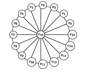
Figure 2: The wheel graph $W_{1,n}$ for $n=16$.

The following theorem answers the question affirmatively for all networks without a cycle.

Theorem 1

If $T$ is a $k^{\prime}$-metric antidimensional tree, then for every $1\leq k\leq k^{\prime}$ there exists a $k$-antiresolving set for $T$.

Some consequences of Theorem 1

Some consequences of the above result in relation to the $(k,\ell)$-anonymity measure are as follows. Note that what is stated below is not the same as the observations in [34].

Clearly, since trees have nodes of degree one (called leaves), it is always possible to identify at least one node of the tree [34]. However, if the network manager introduces some “fake” nodes as leaves, then this advantage for the adversary is avoided. In this sense, the result above asserts that an adversary will never be sure that the set of nodes which it could control will always identify at least one node of the given tree. Another related interesting observation is that for this to happen, the tree must be $k$-metric antidimensional for some $k\geq 2$, otherwise the tree is completely insecure. A characterization of that trees which are $1$-metric antidimensional (graphs that contain only $1$-antiresolving sets) was given in [44].

Note that in the above we claim nothing about what happens if the network does contain a cycle, or how a network manager can break cycles in a network. Note that the topology need not be “fully” controlled by a network manager, but can be influenced by adding extra nodes.

Proof of Theorem 1

We will use the following result from [44] in our proof.

Lemma 2

[44] Any $k$-antiresolving set $S$ in a tree $T$ with $k\geq 2$ induces a connected subgraph of $T$.

Since Problem 1 was shown to be solvable in polynomial time in [9], we may assume that we know the value $k^{\prime}$ for which the tree $T$ is $k^{\prime}$-metric antidimensional. If $k=1$ or $k=k^{\prime}$ then a $k$-antiresolving set for $T$ clearly exists. We may also assume $k>1$, since otherwise our result follows trivially. Suppose that $k=k^{\prime}-1$ and let $S$ be a $k^{\prime}$-antiresolving set of minimum cardinality for $T$. By Lemma 2, $S$ induces a connected subgraph of $T$. Moreover, according to the definition of a $k$-antiresolving set, there exists an equivalence class $Q\in\Pi_{{V\setminus S,-S}}^{=}$ such that $|Q|=k^{\prime}$. Select $v\in S$ such that $\mathsf{Nbr}(v)\setminus S\neq\emptyset$ and let $v_{1},v_{2},\dots,v_{r}\in\mathsf{Nbr}(v)\setminus S$ for some $r\geq 1$. Clearly, the set $A_{1}=\left\{v_{1},v_{2},\dots,v_{r}\right\}$ forms an equivalence class of $\Pi_{{V\setminus S,-S}}^{=}$. Moreover, the set $A_{2}=\bigcup_{i=1}^{r}\mathsf{Nbr}(v_{i})\setminus\{v\}$, if not empty, also forms an equivalence class of $\Pi_{{V\setminus S,-S}}^{=}$. Fig 3 shows two examples which are useful to clarify all the notations of this proof (recall that the eccentricity of a node $v$ is the maximum over the set of distances between $v$ to all other nodes in the graph).

Figure 3: Two auxiliary trees. Notice that eccentricity of $v$ in the subtrees is three in both cases. The set $S$ is a $4$-antiresolving set. The nodes of the subtree $T_{2}$ are shown in bold in both trees.

Assume that $T$ is rooted at node $v$ and, for every $v_{i}\in A_{1}$, let $T_{i}$ be the subtree of $T$ with node set $V(T_{i})$ formed by $v$, $v_{i}$, and the set of descendants of $v_{i}$. Let $e_{i}$ be the eccentricity of $v$ in $T_{i}$ for $1\leq i\leq r$. Moreover, let $A_{j}$ be the subset of nodes $x$ in $\bigcup_{i=1}^{\,r}V(T_{i})$ such that $\mathrm{dist}_{v,x}=j$ for every $1\leq j\leq\max\{e_{i}\,:\;1\leq i\leq r\}$. Observe that each $A_{j}$, with $1\leq j\leq\max\{e_{i}\,:\;1\leq i\leq r\}$, is an equivalence class of $\Pi_{{V\setminus S,-S}}^{=}$ and thus, $|A_{j}|\geq k^{\prime}$ since otherwise $S$ is not a $k^{\prime}$-antiresolving set. Moreover, without loss of generality, we can assume there exists a set $A_{q}$ such that $|A_{q}|=k^{\prime}$ (e.g., in Fig 3 the sets $A_{1}$ and $A_{4}$). If there is no such set, then we choose another node $v^{\prime}$ of $T$ for which this situation happen. If there is no such node $v^{\prime}$ at all, then the cardinality of every equivalence class of $\Pi_{{V\setminus S,-S}}^{=}$ is strictly larger than $k^{\prime}$, which contradicts the definition of a $k^{\prime}$-antiresolving set. We now consider the following situations.

Case 1: $e_{1}=e_{2}=\dots=e_{r}$ (e.g., in Fig 3 (I) all the eccentricities are equal to $3$). Notice that in this case $A_{j}\cap V(T_{i})\neq\emptyset$ for every $1\leq j\leq\max\{e_{i}\,:\;1\leq i\leq r\}$ and every $1\leq i\leq r$. Moreover, there exist $\alpha,\beta$ such that $|A_{\alpha}\cap V(T_{\beta})|=1$ (e.g., in Fig 3 (I) $\alpha=1$ and $\beta$ can take any value between $1$ and $4$). Thus, for the set $S^{\prime}=S\cup V(T_{\beta})$ it follows that $A_{\alpha}\setminus V(T_{\beta})$ is an equivalence class of the equivalence relation $\Pi_{{V\setminus S^{\prime},-S^{\prime}}}^{=}$ and $|A_{\alpha}-V(T_{\beta})|=k^{\prime}-1$. Moreover, for every other equivalence class $X$ of $\Pi_{{V\setminus S^{\prime},-S^{\prime}}}^{=}$ it follows $|X|\geq k^{\prime}-1=k$. Thus, $X$ is a $(k^{\prime}-1)$-antiresolving set. Clearly, $X$ could not be of minimum cardinality.

Case 2: There are at least two subtrees $T_{i}$ and $T_{j}$ such that $e_{i}\neq e_{j}$. Without loss of generality, assume that $e_{1}\leq e_{2}\leq\dots\leq e_{r}$. As in Case 1, there exist $\gamma$ such that $|A_{\gamma}|=k^{\prime}$ (e.g., in Fig 3 (II) $\alpha=3$). Let $S_{1}=S\cup V(T_{1})$ (note that $T_{1}$ is the subtree in which $v$ has the minimum eccentricity). If $|A^{(1)}_{j}|\geq k^{\prime}$ for every $A^{(1)}_{j}=A_{j}\setminus V(T_{1})$ with $1\leq j\leq e_{1}$, then $\gamma>e_{1}$ and thus $S_{1}$ is also a $k^{\prime}$-antiresolving set. Hence, we consider $S_{2}=S_{1}\cup V(T_{2})$ (note that $T_{2}$ is the subtree in which $v$ has the second minimum eccentricity). If $|A^{(2)}_{j}|\geq k^{\prime}$ for every $A^{(2)}_{j}=A^{(1)}_{j}\setminus V(T_{2})$ with $1\leq j\leq e_{2}$, then $\gamma>e_{2}$. Repeating this procedure, we shall find a set $S_{q}=S_{q-1}\cup V(T_{q})$ such that $\gamma\leq e_{q}$ and moreover, $|A_{\alpha^{\prime}}\cap V(T_{\beta^{\prime}})|=1$ for some $1\leq\alpha^{\prime}\leq e_{r}$ and $q\leq\beta^{\prime}\leq r$. Thus, the set $A^{(q+1)}_{j}=A^{(q)}_{j}\setminus V(T_{q+1})$ satisfies $|A^{(q)}_{j}|=k^{\prime}-1$ and consequently $S_{q+1}=S_{q}\cup V(T_{q+1})$ is a $(k^{\prime}-1)$-antiresolving set (e.g., in Fig 3 (II) the process must be done two times, first we remove the nodes in the set $V(T_{1})\setminus\{v\}$ and next we remove the nodes in the set $V(T_{2})\setminus\{v\}$, thereby getting the required $(k^{\prime}-1)$-antiresolving set).

Thus, in both cases we obtain a $(k^{\prime}-1)$-antiresolving set. By using the same procedure and a $(k^{\prime}-1)$-antiresolving set of minimum cardinality, we can find a $(k^{\prime}-2)$-antiresolving set and in general a $k$-antiresolving set for every $2\leq k\leq k^{\prime}-1$, which completes the proof.

3.2 Empirical results

We remind the readers about the assertions in ($\star$), ($\bowtie$) and ($\spadesuit$) while we report our empirical results and related conclusions.

3.2.1 Algorithms for Problems 1–3 (Algorithms I and II)

We obtain an exact solution for Problem 2 by implementing the following algorithm (Algorithm I) devised in [9] by Chatterjee et al.. In this algorithm, an absence of a valid solution is indicated by $\mathpzc{L}_{\mathrm{opt}}^{\geq k}\leftarrow\infty$ and $V_{\mathrm{opt}}^{\geq k}\leftarrow\emptyset$.

(* Algorithm I *)
1.	Compute $\mathbf{d}_{v_{i}}$ for all $i=1,\dots,n$ using any algorithm that solves
	all-pairs-shortest-path problem [12].
2.	$\widehat{\mathpzc{L}_{\mathrm{opt}}^{\geq k}}\leftarrow\infty$ ; $\widehat{V_{\mathrm{opt}}^{\geq k}}\leftarrow\emptyset$
3.	for each $v_{i}\in V$ do
3.1		$V^{\prime}=\left\{v_{i}\right\}$ ; $\mathsf{done}\leftarrow\mathsf{FALSE}$
3.2		while $\big{(}$ $(V\setminus V^{\prime}\neq\emptyset)$ AND $(\mathsf{NOT}\,\,\mathsf{done})$ $\big{)}$ do
3.2.1		compute $\mu\left(\mathcal{D}_{V\setminus V^{\prime},-V^{\prime}}\right)$
3.2.2		if $\Big{(}\,\big{(}\,\mu\left(\mathcal{D}_{V\setminus V^{\prime},-V^{\prime}}\right)\geq k\,\big{)}$ and $\big{(}\,|V^{\prime}|<\widehat{\mathpzc{L}_{\mathrm{opt}}^{\geq k}}\,\big{)}\,\Big{)}$
3.2.3		then       $\widehat{\mathpzc{L}_{\mathrm{opt}}^{\geq k}}\leftarrow|V^{\prime}|$ ; $\widehat{V_{\mathrm{opt}}^{\geq k}}\leftarrow V^{\prime}$ ; $\mathsf{done}\leftarrow\mathsf{TRUE}$
3.2.4		else          let $V_{1},V_{2},\dots,V_{\ell}$ be the only $\ell>0$ equivalence classes
		in $\Pi_{{V\setminus V^{\prime},-V^{\prime}}}^{=}$ such that
		$\left|V_{1}\right|=\dots=\left|V_{\ell}\right|=\mu\left(\mathcal{D}_{V\setminus V^{\prime},-V^{\prime}}\right)$
3.2.5		$V^{\prime}\,\leftarrow\,V^{\prime}\cup\left(\cup_{t=1}^{\ell}V_{t}\right)$
4.	return $\widehat{\mathpzc{L}_{\mathrm{opt}}^{\geq k}}$ and $\widehat{V_{\mathrm{opt}}^{\geq k}}$ as our solution

We obtain exact solutions for Problem 1 and find ${k}_{\mathrm{opt}}$ by using Algorithm I and doing a binary search for the parameter $k$ over the range $\{1,2,\dots,n\}$ to find the largest $k$ such that $V_{\mathrm{opt}}^{\geq k}\neq\emptyset$. This requires using Algorithm I $O(\log n)$ times.

Although Adim_=k is $\mathsf{NP}$-hard for almost all $k$, for $k=1$ we implement the following logarithmic-approximation algorithm devised in [9] by Chatterjee et al. for Adim₌₁ computing $\mathpzc{L}_{\mathrm{opt}}^{=1}$ and $V_{\mathrm{opt}}^{=1}$.

(* Algorithm II *)
1.	Compute $\mathbf{d}_{v_{i}}$ for all $i=1,\dots,n$ using any algorithm that solves
	all-pairs-shortest-path problem [12].
2.	$\widehat{\mathpzc{L}_{\mathrm{opt}}^{=1}}\leftarrow\infty$ ; $\widehat{V_{\mathrm{opt}}^{=1}}\leftarrow\emptyset$
3.	for each node $v_{i}\in V$ do
	3.1	create the following instance of the set-cover problem [28]
		containing $n-1$ elements and $n-1$ sets:
		$\mathcal{U}=\left\{\,a_{v_{j}}\,|\,v_{j}\in V\setminus\left\{v_{i}\right\}\,\right\}$,
		$S_{v_{j}}=\left\{a_{v_{j}}\right\}\cup\left\{a_{v_{\ell}}|\mathrm{dist}_{v_{i},v_{j}}\neq\mathrm{dist}_{v_{\ell},v_{j}}\right\}$ for $j\in\{1,\dots,n\}\setminus\{i\}$
	3.2	if $\cup_{j\in\{1,\dots,n\}\setminus\{i\}}S_{v_{j}}=\mathcal{U}$ then
		3.2.1   run the algorithm of Johnson in [28] for this instance of
		set-cover giving a solution $\mathcal{I}\subseteq\{1,\dots,n\}\setminus\{i\}$
		3.2.2   $V^{\prime}=\left\{\,v_{j}\,|\,j\in\mathcal{I}\,\right\}$
		3.2.3   if $\big{(}\,|V^{\prime}|<\widehat{\mathpzc{L}_{\mathrm{opt}}^{=1}}\,\big{)}$ then $\,\,\,\widehat{\mathpzc{L}_{\mathrm{opt}}^{=1}}\leftarrow\left|V^{\prime}\right|$ ; $\widehat{V_{\mathrm{opt}}^{=1}}\leftarrow V^{\prime}$
4.	return $\widehat{\mathpzc{L}_{\mathrm{opt}}^{=1}}$ and $\widehat{V_{\mathrm{opt}}^{=1}}$ as our solution

3.3 Run-time analyses and implementations of Algorithms I and II

Both Algorithm I and Algorithm II use the all-pairs-shortest-path (Apsp) computation, and this is the step that dominates the theoretical worst-case running time of both the algorithms. The following algorithmic approaches are possible for the all-pairs-shortest-path step:

• For the classical Floyd-Warshall algorithm for Apsp [12], the theoretical worst-case running time of is $O(n^{3})$ when $n$ is the number of nodes in the network. In practice, for larger networks the running time of the Floyd-Warshall algorithm for Apsp can often be improved by using algorithmic engineering tricks such as early termination criteria that are known in the algorithms community.

  For our networks, we found the Floyd-Warshall algorithm with appropriate data structures and algorithmic engineering techniques to be sufficient; one reason for this could be that most of our networks, like many other real-world networks, have a small diameter and thus some computational steps in the Floyd-Warshall algorithm can often be skipped (the diameter of a network can be computed in worst-case $o(n^{3})$ time [47] and in just $O(m)$ time in practice for many real-world networks [13]).

• Repeatedly running breadth-first-search [12] from each node gives a solution of Apsp with a worst-case running time of $O(mn)$, which is better than $O(n^{3})$ if $m=o(n^{2})$, i.e., the network is sparse.

• For specific types of networks, practitioners also consider using other algorithmic approaches, such as repeated use of Dijkstra’s single-source shortest path or Johnson’s algorithm [12], if they are run faster. Both these algorithms have a worst-case running time of $O(n^{2}\log n+nm)$ where $m$ is the number of edges, and therefore run faster than Floyd-Warshall algorithm in the worst case if $m=o(n^{2})$.

• Using graph compression techniques, it is possible to design a $O(n^{3}/\log n)$ worst-case time algorithm for Apsp [16].

• Using fast matrix multiplication algorithms, Apsp can be solved in $O(n^{2.376})$ time [19, 20, 41] using Coppersmith and Winograd’s matrix multiplication result [11].

For increasing the efficiency and speed of the algorithms we used various data structures such as STL nested maps and vectors to improve comparisons and lookup operations. Furthermore, for Algorithm I, we prematurely terminate the algorithm if $|V_{\mathrm{opt}}|$ reaches $1$ as $1$ is the smallest value of the size of attacker nodes.

Finally, just like the measures in this article, the Apsp computation is unavoidable for a large variety of other geodesic-based network properties that are often used for real networks such as the betweenness centrality, closeness centrality or Gromov-hyperbolicity measure, and there is a vast amount of literature that apply such measures to large networks (e.g., see [7, 46, 3, 35, 36, 27]).

3.4 Scalability of the privacy measure with respect to the size of network

We have tested computation of the privacy measures for graphs up to $1000$ nodes. For Algorithm I, we found that the running time for computing the measure for an individual network ranges from $1$ minute or less (for smaller sparser networks) to about $10$ to $20$ minutes (for larger denser networks). For Algorithm-II the running time was mostly in the order of a few minutes.

However, for much larger networks than what has been used in this paper, we would recommend a more careful implementation, specially for Algorithm I, to achieve a more time efficient implementation. Towards this goal, we provide the following suggestions in relation to computing the measures for larger networks:

• For larger networks, it would be advisable to use the fastest possible implementation of the all-pairs-shortest-paths algorithm. This is a well-known problem that admits a variety of algorithms some of which are especially more efficient on non-dense networks and moreover in practice the running times of many of these algorithms can be significantly improved by using several algorithmic engineering tricks (early termination criteria, efficient data structures etc.) that are known in the algorithmic implementation community. Also, if the same network is used for more than one privacy measure computation, it is certainly advisable to store the all-pairs-shortest-path data and re-use them instead of computing them afresh every time.

• Although our simulation did not need it, for larger networks the relevant set operations needed in Algorithms I and II can be implemented more efficiently, for example using the well-known data structures for disjoint sets (e.g., see [18] for a survey).

• For extremely large networks, say dense networks containing millions of nodes, it may be advisable to use a suitable sampling method such as in [31] to sample appropriate sub-graphs of smaller size, and use the measures computed on these sub-graphs to statistically estimate the value of the measures on the entire graph.

3.4.1 Synthetic networks: models and algorithmic generations

Unfortunately, there is no single universally agreed upon synthetic network model that faithfully reproduces all networks in various application domains (e.g., see [42, 29, 1]). In fact, there are some results that cast doubt if a true generative network model can even be known unambiguously. Thus, it is very customary in the network research community to draw conclusions of the following type:

“For those real-world networks generated by such-and-such model, we can conclude that $\ldots\ldots$”

We use two major types of synthetic networks, namely the Erdös-Rényi random networks and the scale-free random networks generated by the Barábasi-Albert preferential-attachment model [6]. Although the Erdös-Rényi network model has been used by prior network researchers as a real-network model in several application domains (e.g., see [39, 17, 33, 8]) it is also known that this particular model is probably not very good a model for real networks in many other application domains. Thus, we also consider networks generated by the scale-free random network model which is more widely considered to be a real-network model in many network applications (e.g., see  [6, 4, 10, 45, 2]).

Erdös-Rényi model This is the classical undirected Erdös-Rényi model $G(n,p)$, where $n$ is the number of nodes and every possible edge in the network is selected independently with a probability of $p$. The average degree of any node in $G(n,p)$ is $(n-1)p\approx np$, leading to $\frac{n(n-1)p}{2}\approx\frac{n^{2}p}{2}$ as the average number of edges in the network. Our privacy measures assume that the given graph is connected since one connected component has no influence on the privacy of another connected component. Thus, it is imperative to select only those combinations of $n$ and $p$ that keeps the graph connected by keeping the average degree of every node to be at least $1$. However, we actually need to make sure that the average degree is at least $2$ since, for example, $\mathpzc{L}_{\mathrm{opt}}^{=1}$ is trivially equal to $1$ otherwise. This implies that at the very least we must ensure that $(n-1)p\geq 2$, or roughly $np\geq 2$. However, in practice, while generating the actual random networks one may need to select a $p$ that is slightly higher (in our case, $np\geq 2.5$). Note that the giant-component formation in ER networks happens around $np\approx 1$, so we are indeed further away from this phenomenon where slight variations in $p$ cause abrupt changes in topological behavior of the network. We used the following four combinations of $n$ and $p$ to generate our synthetic networks to capture a smaller average degree of $2.5$, a modest average degree of $5$ and a larger average degree of $10$:

$n$ $=$ $500$ $p$ $=$ $0.005$ $np$ $=$ $2.5$        $n$ $=$ $500$ $p$ $=$ $0.01$ $np$ $=$ $5$        $n$ $=$ $1000$ $p$ $=$ $0.005$ $np$ $=$ $5$        $n$ $=$ $1000$ $p$ $=$ $0.01$ $np$ $=$ $10$

For $n=500$ (respectively, for $n=1000$) we generated $1000$ random networks (respectively, $100$ random networks) for each corresponding value of $p$, and then calculated relevant statistics using Algorithms I and II.

Scale-free model We use the Barábasi-Albert preferential-attachment model  [6] to generate random scale-free networks. The algorithm for generating a random scale-free $G(n,q)$,where $n$ is number of nodes and $q\ll n$ is the number of connections each new node makes, is as follows:

• Initialize $G$ to have $q$ nodes and no edges. Add these nodes to a “list of repeated nodes”.

• Repeat the following steps till $G$ has $n$ nodes:

  • Randomly select $q$ distinct nodes, say $u_{1},\dots,u_{q}$, from the list of repeated nodes.

  • Add a new node $w$ and undirected edges $\{w,u_{1}\},\dots,\{w,u_{q}\}$ in $G$.

  • Add $w$ and $u_{1},\dots,u_{q}$ to the current list of repeated nodes.

The larger the $q$ is, the more dense is the network $G(n,q)$. We used the following four combinations of $n$ and $q$ to generate our synthetic scale-free networks:

$n$ $=$ $500$ $q$ $=$ $5$        $n$ $=$ $500$ $q$ $=$ $10$        $n$ $=$ $1000$ $q$ $=$ $5$        $n$ $=$ $1000$ $q$ $=$ $10$

For $n=500$ (respectively, for $n=1000$) we generated $1000$ random networks (respectively, $100$ random networks) for each corresponding value of $q$, and then calculated relevant statistics using Algorithms I and II.

3.4.2 Real networks

Table 3: List of real social networks studied in this paper.

Name	# of		Description
	nodes	edges
(A) Zachary Karate Club [48]	$34$	$78$	Network of friendships between $34$ members of a karate club at a US university in the $1970$s
(B) San Juan Community [32]	$75$	$144$	Network for visiting relations between families living in farms in the neighborhood San Juan Sur, Costa Rica, $1948$
(C) Jazz Musician Network [22]	$198$	$2842$	A social network of Jazz musicians
(D) University Rovira i Virgili emails [23]	$1133$	$10903$	the network of e-mail interchanges between members of the University Rovira i Virgili
(E) Enron Email Data set [15]	$1088$	$1767$	Enron email network
(F) Email Eu core [37]	$986$	$24989$	Emails from a large European research institution
(G) UC Irvine College Message platform [38]	$1896$	$59835$	Messages on a Facebook-like platform at UC-Irvine
(H) Hamsterster friendships  [24]	$1788$	$12476$	This Network contains friendships between users of the website hamsterster.com

Table 3 shows the list of eight well-known unweighted social networks that we investigated. All the networks except one were undirected; for the only directed UC Irvine College Message platform network, we ignored the direction of edges. For each network the largest connected component was selected and tested.

3.4.3 Results for real networks in Table 3

Results for Adim and Adim_≥k Table 4 shows the results for Adim via applying Algorithm I to these networks. From these results we may conclude:

①

For all networks except the “Enron Email Data” network, an attacker needs to control only one suitable node of the network to uniquely re-identify (based on the metric representation) a significant percentage of nodes in the network (ranging from $2.6\%$ of nodes for the “University Rovira i Virgili emails” network to $26.5\%$ of nodes for the “Zachary Karate Club” network).

②

For all networks except the “Enron Email Data” network, the minimum privacy violation probability guarantee is significantly further from zero (ranging from $0.019$ for the “UC Irvine College Message platform” network to $0.25$ for the “Hamsterster friendships” network). The minimum privacy violation probability guarantee for the “Hamsterster friendships” network is significantly higher than all other networks.

③

The “Zachary Karate Club” and the “San Juan Community” networks are more vulnerable to privacy attacks in terms of the percentage of nodes in the networks whose privacy can be violated by the adversary.

Table 4: Results for Adim using Algorithm I. $n$ is the number of nodes and ${k}_{\mathrm{opt}}$ is the largest value of $k$ such that $V_{\mathrm{opt}}^{\geq k}\neq\emptyset$ (cf. Problem 1).

Name	$n$	${k}_{\mathrm{opt}}$	${p}_{\mathrm{opt}}=\nicefrac{{1}}{{{k}_{\mathrm{opt}}}}$	$\mathpzc{L}_{\mathrm{opt}}^{\geq{k}_{\mathrm{opt}}}=\mathpzc{L}_{\mathrm{opt}}^{={k}_{\mathrm{opt}}}$	$\frac{{k}_{\mathrm{opt}}}{n}$
(A) Zachary Karate Club	$34$	$9\,\,$	$0.111$	$1$	$26.5\%\,\,\,\,\,$
(B) San Juan Community	$75$	$7\,\,$	$0.143$	$1$	$9.3\%\,\,\,\,\,$
(C) Jazz Musician Network	$198$	$12\,\,$	$0.084$	$1$	$6.0\%\,\,\,\,\,$
(D) University Rovira i Virgili emails	$1133$	$29\,\,$	$0.035$	$1$	$2.6\%\,\,\,\,\,$
(E) Enron Email Data set	$1088$	$153\,\,$	$0.007$	$935$	$14.1\%\,\,\,\,\,$
(F) Email Eu core	$986$	$39\,\,$	$0.026$	$1$	$3.4\%\,\,\,\,\,$
(G) UC Irvine College Message platform	$1896$	$55\,\,$	$0.019$	$1$	$2.9\%\,\,\,\,\,$
(H) Hamsterster friendships	$1788$	$4\,\,$	$0.25$	$1$	$0.22\%\,\,\,\,\,$

For the “Enron Email Data” network, $\mathpzc{L}_{\mathrm{opt}}^{\geq{k}_{\mathrm{opt}}}=935$ implies that even to achieve a modest value of ${p}_{\mathrm{opt}}=0.007$ an adversary needs to control a large percentage (at least $\frac{935\times 100}{1088}\%\approx 86\%$) of its nodes, a possibility unlikely to happen in practice. Thus, we continue further investigation about this network to check if a value of $k$ somewhat smaller than ${k}_{\mathrm{opt}}$ may allow a sufficiently steep decline in the number of nodes that the attacker need to control, and report the values of $\mathpzc{L}_{\mathrm{opt}}^{\geq k}$ corresponding to relevant values of $k>1$ in Table 5. As can be seen, the values of $\mathpzc{L}_{\mathrm{opt}}^{\geq k}$ does not decline unless $k$ is really further away from ${k}_{\mathrm{opt}}$, leading us to conclude the following:

④

For the “Enron Email Data” network, privacy violation of a large number of nodes of the network by an attacker cannot be guaranteed in a practical sense (i.e., without gaining control of a large number of nodes).

Table 5: Values of $\mathpzc{L}_{\mathrm{opt}}^{\geq k}$ corresponding to values for $k>1$ for “Enron Email Data” network. Only those values of $k>1$ for which $\mathpzc{L}_{\mathrm{opt}}^{\geq k}\neq\mathpzc{L}_{\mathrm{opt}}^{\geq k-1}$ are shown.

(E) Enron Email Data set $k$ $4$ $5$ $10$ $20$ $40$ $60$ $100$ $120$ $153$ $p_{k}=\nicefrac{{1}}{{k}}$ $0.25$ $0.2$ $0.1$ $0.05$ $0.025$ $0.017$ $0.01$ $0.009$ $0.007$ $\mathpzc{L}_{\mathrm{opt}}^{\geq k}$ $1$ $334$ $463$ $567$ $683$ $842$ $935$ $935$ $935$

Results for Adim₌₁ Algorithm II returns $\mathpzc{L}_{\mathrm{opt}}^{=1}=1$ for all of our networks except the “Hamsterster friendships” network. For the “Hamsterster friendships” network, Algorithm II returns $\mathpzc{L}_{\mathrm{opt}}^{=1}=2$. Thus, we conclude:

⑤

For all the real networks except the “Hamsterster friendships” network, an adversary controlling just one suitable node may uniquely re-identify (based on the metric representation) one other node in the network with certainty (i.e., with a probability of $1$). For the “Hamsterster friendships” network, the same conclusion holds provided the adversary controls two suitable nodes.

3.4.4 Results for Erdös-Rényi synthetic networks

Results for Adim_≥k Table 6 shows the results for Adim_≥k via applying Algorithm I to these networks. From these results we may conclude:

⑥

For most synthetic Erdös-Rényi networks, ${k}_{\mathrm{opt}}$ is a value that is much smaller compared to the number of nodes $n$. Thus, for our synthetic Erdös-Rényi networks, with high probability privacy violation of a large number of nodes of the network by an attacker cannot be achieved.

⑦

The values of $\frac{{k}_{\mathrm{opt}}}{n}$ for denser Erdös-Rényi networks (corresponding to $p=0.01$) is about $75\%$ higher that those for sparser Erdös-Rényi networks (corresponding to $p=0.005$) irrespective of the number of nodes. Thus, we conclude that our sparser synthetic Erdös-Rényi networks are more privacy-secure compared to their denser counter-parts.

Table 6: Results for Adim_≥k using Algorithm I for classical Erdös-Rényi model $G(n,p)$. ${k}_{\mathrm{opt}}$ is the largest value of $k$ such that $V_{\mathrm{opt}}^{\geq k}\neq\emptyset$ (cf. Problem 1). The %-values indicate the percentage of the generated networks for those particular values of ${k}_{\mathrm{opt}}$ (e.g., for $n=500$ and $p=0.005$, $980$ out of the $1000$ networks have ${k}_{\mathrm{opt}}\geq 5$).

Network
parameters
$n$	$p$
$500$	$0.005$	${k}_{\mathrm{opt}}$	$\geq 4$	$\geq 5$	$\geq 6$	$\geq 7$	$\geq 8$	$\geq 9$	$\geq 10$	$>10$
		${p}_{\mathrm{opt}}=\nicefrac{{1}}{{{k}_{\mathrm{opt}}}}$	$\leq 0.25$	$\leq 0.2$	$\leq 0.166$	$\leq 0.142$	$\leq 0.125$	$\leq 0.111$	$\leq 0.1$	$<0.1$
		% of networks	$100\%$	$98\%$	$81.8\%$	$54.6\%$	$21.5\%$	$8\%$	$3\%$	$1\%$
		At least $90\%$ of networks have ${k}_{\mathrm{opt}}\leq 8$ and $\frac{{k}_{\mathrm{opt}}}{n}\leq 0.016$
$500$	$0.010$	${k}_{\mathrm{opt}}$	$\geq 9$	$\geq 10$	$\geq 11$	$\geq 12$	$\geq 13$	$\geq 14$	$\geq 15$	$>15$
		${p}_{\mathrm{opt}}=\nicefrac{{1}}{{{k}_{\mathrm{opt}}}}$	$\leq 0.11$	$\leq 0.1$	$\leq 0.09$	$\leq 0.083$	$\leq 0.077$	$\leq 0.071$	$\leq 0.066$	$<0.066$
		% of networks	$100\%$	$98\%$	$94\%$	$81.4\%$	$49.4\%$	$21.4\%$	$6.8\%$	$0.6\%$
		At least $90\%$ of networks have ${k}_{\mathrm{opt}}\leq 14$ and $\frac{{k}_{\mathrm{opt}}}{n}\leq 0.028$
$1000$	$0.005$	${k}_{\mathrm{opt}}$	$\geq 10$	$\geq 11$	$\geq 12$	$\geq 13$	$\geq 14$	$>14$
		${p}_{\mathrm{opt}}=\nicefrac{{1}}{{{k}_{\mathrm{opt}}}}$	$\leq 0.1$	$\leq 0.09$	$\leq 0.083$	$\leq 0.077$	$\leq 0.071$	$<0.066$
		% of networks	$100\%$	$99\%$	$65\%$	$16\%$	$7\%$	$1\%$
		At least $90\%$ of networks have ${k}_{\mathrm{opt}}\leq 13$ and $\frac{{k}_{\mathrm{opt}}}{n}\leq 0.013$
$1000$	$0.010$	${k}_{\mathrm{opt}}$	$\geq 18$	$\geq 19$	$\geq 20$	$\geq 21$	$\geq 22$	$\geq 23$	$\geq 24$	$>24$
		${p}_{\mathrm{opt}}=\nicefrac{{1}}{{{k}_{\mathrm{opt}}}}$	$\leq 0.055$	$\leq 0.052$	$\leq 0.05$	$\leq 0.047$	$\leq 0.045$	$\leq 0.043$	$\leq 0.041$	$<0.041$
		% of networks	$100\%$	$99\%$	$90\%$	$75\%$	$47\%$	$26\%$	$9\%$	$1\%$
		At least $90\%$ of networks have ${k}_{\mathrm{opt}}\leq 23$ and $\frac{{k}_{\mathrm{opt}}}{n}\leq 0.023$

Results for Adim₌₁ Table 7 shows the result of our experiments of computation of $\mathpzc{L}_{\mathrm{opt}}^{=1}$ using Algorithm II. From these results, we conclude:

⑧

For our synthetic Erdös-Rényi networks, with high probability an adversary controlling at most two nodes may uniquely re-identify (based on the metric representation) at least one other node in the network.

Table 7: Results for Adim₌₁ using Algorithm II for classical Erdös-Rényi model $G(n,p)$. The %-values indicate the percentage of the generated networks that have the corresponding value of $\mathpzc{L}_{\mathrm{opt}}^{=1}$ (e.g., for $n=500$ and $p=0.01$, $920$ out of the $1000$ networks have $\mathpzc{L}_{\mathrm{opt}}^{=1}=1$).

Network parameters		$\mathpzc{L}_{\mathrm{opt}}^{=1}$
$n$	$p$	$1$	$2$	$>2$
$500$	$0.01$	$92$%	$7$%	$1$%
$500$	$0.005$	$5.9$%	$89.3$%	$4.8$%
$1000$	$0.01$	$8$%	$90$%	$2$%
$1000$	$0.005$	$5$%	$93$%	$1$%

Table 8: Results for Adim_≥k using Algorithm I for the Barábasi-Albert preferential-attachment scale-free model $G(n,q)$. ${k}_{\mathrm{opt}}$ is the largest value of $k$ such that $V_{\mathrm{opt}}^{\geq k}\neq\emptyset$ (cf. Problem 1). The %-values indicate the percentage of the generated networks for those particular values of ${k}_{\mathrm{opt}}$ (e.g., for $n=500$ and $q=5$, $990$ out of the $1000$ networks have ${k}_{\mathrm{opt}}\geq 50$).

Network
parameters
$n$	$q$
$500$	$5$	${k}_{\mathrm{opt}}$	$\geq 49$	$\geq 50$	$\geq 55$	$\geq 60$	$\geq 65$	$\geq 70$	$>70$
		${p}_{\mathrm{opt}}=\nicefrac{{1}}{{{k}_{\mathrm{opt}}}}$	$\leq 0.0204$	$\leq 0.02$	$\leq 0.018$	$\leq 0.016$	$\leq 0.015$	$\leq 0.014$	$<0.014$
		% of networks	$100\%$	$99\%$	$97\%$	$89\%$	$42\%$	$10\%$	$6\%$
		At least $90\%$ of networks have ${k}_{\mathrm{opt}}\leq 65$ and $\frac{{k}_{\mathrm{opt}}}{n}\leq 0.13$
$500$	$10$	${k}_{\mathrm{opt}}$	$\geq 45$	$\geq 60$	$\geq 80$	$\geq 100$	$\geq 120$	$\geq 140$	$>140$
		${p}_{\mathrm{opt}}=\nicefrac{{1}}{{{k}_{\mathrm{opt}}}}$	$\leq 0.022$	$\leq 0.016$	$\leq 0.0125$	$\leq 0.001$	$\leq 0.008$	$\leq 0.007$	$<0.007$
		% of networks	$100\%$	$50\%$	$48\%$	$47\%$	$27\%$	$5\%$	$4\%$
		At least $95\%$ of networks have ${k}_{\mathrm{opt}}\leq 120$ and $\frac{{k}_{\mathrm{opt}}}{n}\leq 0.24$
$1000$	$5$	${k}_{\mathrm{opt}}$	$\geq 88$	$\geq 90$	$\geq 100$	$\geq 110$	$\geq 120$	$\geq 130$	$\geq 135$
		${p}_{\mathrm{opt}}=\nicefrac{{1}}{{{k}_{\mathrm{opt}}}}$	$\leq 0.011$	$\leq 0.010$	$\leq 0.001$	$\leq 0.009$	$\leq 0.008$	$\leq 0.007$	$\leq 0.0074$
		% of networks	$100\%$	$98\%$	$94\%$	$66\%$	$32\%$	$11\%$	$1\%$
		At least $89\%$ of networks have ${k}_{\mathrm{opt}}\leq 120$ and $\frac{{k}_{\mathrm{opt}}}{n}\leq 0.12$
$1000$	$10$	${k}_{\mathrm{opt}}$	$\geq 86$	$\geq 88$	$\geq 90$	$\geq 92$	$\geq 94$	$\geq 96$	$\geq 98$	$>100$
		${p}_{\mathrm{opt}}=\nicefrac{{1}}{{{k}_{\mathrm{opt}}}}$	$\leq 0.0116$	$\leq 0.0113$	$\leq 0.0111$	$\leq 0.0108$	$\leq 0.0106$	$\leq 0.0104$	$\leq 0.0102$	$<0.001$
		% of networks	$100\%$	$77\%$	$67\%$	$56\%$	$43\%$	$30\%$	$13\%$	$3\%$
		At least $87\%$ of networks have ${k}_{\mathrm{opt}}\leq 96$ and $\frac{{k}_{\mathrm{opt}}}{n}\leq 0.096$

3.4.5 Results for scale-free synthetic networks

Results for Adim_≥k Table 8 shows the results for Adim_≥k via applying Algorithm I to these networks. From these results we may conclude:

⑨

The value of ${k}_{\mathrm{opt}}$ relative to the size $n$ of the network is much larger for synthetic scale-free networks compared to those for the synthetic Erdös-Rényi networks. Thus, compared to synthetic Erdös-Rényi networks, synthetic scale-free networks may allow privacy violation of a larger number of nodes of the network by an attacker.

⑩

Unlike the synthetic Erdös-Rényi networks, the values of $\frac{{k}_{\mathrm{opt}}}{n}$ for denser scale-free networks (corresponding to $q=10$) may be smaller or larger than those for sparser scale-free networks (corresponding to $q=5$). Thus, density of scale-free networks does not seem to be well-correlated to privacy-security of these networks.

Results for Adim₌₁ Table 9 shows the result of our experiments of computation of $\mathpzc{L}_{\mathrm{opt}}^{=1}$ using Algorithm II. From these results, we conclude:

Similar to synthetic synthetic Erdös-Rényi networks, for synthetic scale-free networks also with high probability an adversary controlling at most two nodes may uniquely re-identify (based on the metric representation) at least one other node in the network.

Table 9: Results for Adim₌₁ using Algorithm II for the Barábasi-Albert preferential-attachment scale-free model $G(n,q)$. The %-values indicate the percentage of the generated networks that have the corresponding value of $\mathpzc{L}_{\mathrm{opt}}^{=1}$ (e.g., for $n=500$ and $q=5$, $990$ out of the $1000$ networks have $\mathpzc{L}_{\mathrm{opt}}^{=1}=2$).

Network parameters		$\mathpzc{L}_{\mathrm{opt}}^{=1}$
$n$	$q$	$2$	$>2$
$500$	$5$	$99$%	$1$%
$500$	$10$	$99.5$%	$0.5$%
$1000$	$5$	$99$%	$1$%
$1000$	$10$	$99$%	$1$%

4 Conclusion

Rapid evolution of popular social networks such as Facebook and Twitter have rendered modern society heavily dependent on such virtual platforms for their day-to-day operation. However, the many benefits accrued by such online networked systems are not necessarily cost-free since a malicious entity may compromise privacy of users of these social networks for harmful purposes that may result in the disclosure of sensitive attributes of these networks. In this article, we investigated, both theoretically and empirically, quantifications of privacy violation measures of large networks under active attacks. Our theoretical result indicates that the network manager responsible for prevention of privacy violation must be very careful in designing the network if its topology does not contain a cycle, while our empirical results shed light on privacy violation properties of eight real social networks as well as synthetic networks generated by the classical Erdö-Rènyi model. We believe that our results will stimulate much needed further research on quantifying and computing privacy measures for networks.

5 Acknowledgements

We thank the anonymous reviewers for their helpful comments. B.D. and N.M. thankfully acknowledges partially support from NSF grant IIS-1160995. This research was partially done while I.G.Y. was visiting the University of Illinois at Chicago, USA, supported by “Ministerio de Educación, Cultura y Deporte”, Spain, under the “José Castillejo” program for young researchers (reference number: CAS15/00007).

References

- [1] Y. Achiam, I. Yahav and D. G. Schwartz, Why not scale free? Simulating company ego networks on Twitter. IEEE/ACM International Conference on Advances in Social Networks Analysis and Mining, San Francisco, CA, 174-177, 2016.
- [2] R. Albert and A. L. Barabási, Statistical mechanics of complex networks. Reviews of Modern Physics, 74(1), 47-97, 2002.
- [3] R. Albert, B. DasGupta and N. Mobasheri, Topological implications of negative curvature for biological and social networks. Physical Review E, 89(3), 032811, 2014.
- [4] H. Amini, R. Cont and A. Minca, Resilience to contagion in financial networks. Mathematical Finance, 26(2), 329-365, 2016.
- [5] L. Backstrom, C. Dwork and J. Kleinberg, Wherefore art thou r3579x?: anonymized social networks, hidden patterns, and structural steganography. Proc. International Conference on World Wide Web, 181-190, New York, NY, USA, 2007.
- [6] A. L. Barábasi and R. Albert, Emergence of scaling in random networks. Science, 286, 509-512, 1999.
- [7] C. Biscaro and C. Giupponi, Co-Authorship and Bibliographic Coupling Network Effects on Citations. PLoS ONE 9(6): e99502, 2014.
- [8] D. S. Callaway, M. E. J. Newman, S. H. Strogatz and D. J. Watts, Network robustness and fragility: percolation on random graphs. Physical Review Letters, 85, 5468-5471, 2000.
- [9] T. Chatterjee, B. DasGupta, N. Mobasheri, V. Srinivasan and I. G. Yero, On the computational complexities of three privacy measures for large networks under active attack. arXiv:1607.01438 [cs.CC], 2016.
- [10] R. Cont, A. Moussa and E. B. Santos, Network Structure and Systemic Risk in Banking Systems. In J. Fouque and J. Langsam (Eds.), Handbook on Systemic Risk, Cambridge University Press, 327-368, 2013.
- [11] D. Coppersmith and S. Winograd, Matrix multiplication via arithmetic progressions. Journal of Symbolic Computation, 9, 251-280, 1990.
- [12] T. H. Cormen, C. E. Leiserson, R. L. Rivest and C. Stein, Introduction to algorithms. The MIT Press, 2001.
- [13] P. Crescenzi, R. Grossi, M. Habib, L. Lanzi and A. Marino, On computing the diameter of real-world undirected graphs. Theoretical Computer Science, 514, 84-95, 2013.
- [14] B. DasGupta B and N. Mobasheri, On optimal approximability results for computing the strong metric dimension. Discrete Applied Mathematics, 221, 18-24, 2017.
- [15] Enron email network, available from UC Berkeley Enron Email Analysis website http://bailando.sims.berkeley.edu/enron_email.html (see also https://www.cs.uic.edu/~dasgupta/network-data/).
- [16] T. Feder and R. Motwani, Clique partitions, graph compression and speeding-up algorithms. Journal of Computer and System Sciences, 51, 261-272, 1995.
- [17] P. Gai and S. Kapadia, Contagion in financial networks. Proc. R. Soc. A, 466(2120), 2401-2423, 2010.
- [18] Z. Galil and G. Italiano, Data structures and algorithms for disjoint set union problems. ACM Computing Surveys, 23, 319-344, 1991.
- [19] Z. Galil and O. Margalit, All pairs shortest distances for graphs with small integer length edges. Information and Computation, 134, 103-139, 1997.
- [20] Z. Galil and O. Margalit, All pairs shortest paths for graphs with small integer length edges. Journal of Computer and System Sciences, 54, 243-254, 1997.
- [21] M. Gast, M. Hauptmann and M. Karpinski, Inapproximability of dominating set on power law graphs. Theoretical Computer Science, 562, 436-452, 2015.
- [22] P. Gleiser and L. Danon, Community structure in Jazz. Advances in Complex Systems, 6(4), 565-573, 2003.
- [23] R. Guimera, L. Danon, A. Diaz-Guilera, F. Giralt and A. Arenas, Self-similar community structure in a network of human interactions. Physical Review E, 68, 065103, 2003.
- [24] Hamsterster friendships network dataset — KONECT, 2017, see http://konect.uni-koblenz.de/networks/petster-friendships-hamster.
- [25] M. Hauptmann, R. Schmied and C. Viehmann, Approximation complexity of metric dimension problem. Journal of Discrete Algorithms, 14, 214-222, 2012.
- [26] M. Hay, G. Miklau, D. Jensen, D. Towsley and P. Weis, Resisting structural re-identification in anonymized social networks. VLDB Journal, 1(1), 102-114, 2008.
- [27] P. Holme, B. J. Kim, C. N. Yoon and S. K. Han, Attack vulnerability of complex networks. Physical Review E, 65, 056109, 2002.
- [28] D. S. Johnson, Approximation algorithms for combinatorial problems. Journal of Computer and System Sciences, 9, 256-278, 1974.
- [29] R. Khanin and E. Wit, How scale-free are biological networks. Journal of Computational Biology, 13(3), 810-818, 2006.
- [30] S. Khuller, B. Raghavachari and A. Rosenfeld, Landmarks in graphs. Discrete Applied Mathematics, 70(3), 217-229, 1996.
- [31] J. Leskovec and C. Faloutsos, Sampling from Large Graphs. ACM SIGKDD International Conference on Knowledge Discovery and Data Mining, 631-636, 2006.
- [32] C. P. Loomis, J. O. Morales, R. A. Clifford and O. E. Leonard, Turrialba: social systems and the introduction of change. The Free Press, Glencoe, IL, p. 45 and 78, 1953.
- [33] S. Markose, S. Giansante, M. Gatkowski and A. R. Shaghaghi, Too interconnected to fail: financial contagion and systemic risk in network model of CDS and other credit enhancement obligations of US banks. Economics Discussion Papers, Department of Economics, University of Essex, 683, 2009.
- [34] S. Mauw, R. Trujillo-Rasua and B. Xuan, Counteracting active attacks in social network graphs. Proceedings of the 30th IFIP Annual Conference on Data and Applications Security and Privacy, 9766, 233-248, 2017.
- [35] M. E. J. Newman, The structure and function of complex networks. SIAM Review, 45, 167-256, 2003.
- [36] M. E. J. Newman, Scientific collaboration networks: II. Shortest paths, weighted networks, and centrality. Physical Review E, 64, 016132, 2001.
- [37] A. Paranjape, A. R. Benson and J. Leskovec, Motifs in temporal networks. Proceedings of the Tenth ACM International Conference on Web Search and Data Mining, 2017.
- [38] P. Panzarasa, T. Opsahl and K. M. Carley, Patterns and dynamics of users’ behavior and interaction: network analysis of an online community. Journal of the American Society for Information Science and Technology, 60(5), 911-932, 2009.
- [39] A. Sachs, Completeness interconnectedness and distribution of interbank exposures - a parameterized analysis of the stability of financial networks. Quantitative Finance, 14(9), 1677-1692, 2014.
- [40] A. Salem, Y. Zhang, M. Humbert, M. Fritz and M. Backes, ML-Leaks: Model and Data Independent Membership Inference Attacks and Defenses on Machine Learning Models. arXiv:1806.01246, 2018.
- [41] R. Seidel, On the all-pairs-shortest-path problem in unweighted undirected graphs. Journal of Computer and System Sciences, 51, 400-403, 1995.
- [42] M. P. H. Stumpf, C. Wiuf and R. M. May, Subnets of scale-free networks are not scale-free: Sampling properties of networks. Proceedings of the National Academy of Sciences, 102(12), 4221-4224, 2005.
- [43] R. Trujillo-Rasua and I. G. Yero, -metric antidimension: a privacy measure for social graphs. Information Sciences, 328, 403-417, 2016.
- [44] R. Trujillo-Rasua and I. G. Yero, Characterizing -metric antidimensional trees and unicyclic graphs. The Computer Journal, 59(8), 1264-1273, 2016.
- [45] A. Wagner, Estimating coarse gene network structure from large-scale gene perturbation data. Genome Research, 12, 309-315, 2002.
- [46] S. Wasserman and K. Faust, Social Network Analysis. Cambridge University Press, Cambridge, 1994.
- [47] R. Yuster, Computing the diameter polynomially faster than APSP. arXiv:1011.6181v2, 2011.
- [48] W. W. Zachary, An information flow model for conflict and fission in small groups. Journal of Anthropological Research, 33, 452-473, 1977.
- [49] C. Zhang and Y. Gao, On the Complexity of k-Metric Antidimension Problem and the Size of k-Antiresolving Sets in Random Graphs. In Y. Cao and J. Chen (Eds.), COCOON 2017, LNCS 10392, 555-567, Springer, 2017.
- [50] T. Zhang, Z. He and R. B. Lee, Privacy-preserving Machine Learning through Data Obfuscation. arXiv:1807.01860, 2018.
- [51] M. Zito, Greedy Algorithms for Minimisation Problems in Random Regular Graphs. Proc. Annuual European Symposium on Algorithms, 525-536, 2001.