Analysis of Dynamic Memory Bandwidth Regulation in Multi-core Real-Time Systems

Abstract

One of the primary sources of unpredictability in modern multi-core embedded systems is contention over shared memory resources, such as caches, interconnects, and DRAM. Despite significant achievements in the design and analysis of multi-core systems, there is a need for a theoretical framework that can be used to reason on the worst-case behavior of real-time workload when both processors and memory resources are subject to scheduling decisions.

In this paper, we focus our attention on dynamic allocation of main memory bandwidth. In particular, we study how to determine the worst-case response time of tasks spanning through a sequence of time intervals, each with a different bandwidth-to-core assignment. We show that the response time computation can be reduced to a maximization problem over assignment of memory requests to different time intervals, and we provide an efficient way to solve such problem. As a case study, we then demonstrate how our proposed analysis can be used to improve the schedulability of Integrated Modular Avionics systems in the presence of memory-intensive workload.

I Introduction

Over the last decade, multi-core systems have rapidly increased in popularity and they are now the de-facto standard in the embedded computing industry. Multi-core systems are significantly more challenging to analyze compared to their single-core counterparts due to the extensive sharing of hardware resources among logically independent execution flows. The primary source of performance unpredictability, in this class of systems, can be identified as the memory hierarchy. In fact, the memory hierarchy in multi-core platforms is comprised of a number of components that are concurrently accessed by multiple cores. These include: multi-level CPU caches, shared memory controllers and DRAM banks, and shared I/O devices. The interplay of accesses originated by multiple cores has a direct impact on the timing of subsequent memory accesses. The resulting temporal variability is in the range of multiple orders of magnitude, meaning that inaccurate performance modeling and analysis can lead to overly pessimistic worst-case execution time (WCET) estimates.

Despite the remarkable achievements in the analysis of hard real-time workload on multi-core systems, there is a fundamental lack of self-contained theoretical frameworks that can be used to reason on the schedulability of a generic multi-core hard real-time workload when both CPU and memory resources are subject to scheduling decisions. In fact, while consolidated techniques are used to reason about CPU scheduling, comparatively less general results are available to reason on memory scheduling. An even slimmer body of works has provided general results to reason on co-scheduling of CPU and memory. The majority of works in this area assume fixed assignment of memory resources to CPUs.

Memory Scheduling: there are two dimensions to the problem of assigning memory resources to applications. The first dimension is space scheduling, concerning the allocation over time of memory space (e.g., cache lines, DRAM banks, scratchpad pages). A second dimension is temporal scheduling, i.e., scheduling of access to a shared memory interface (e.g., an interconnect, a bus, or a memory controller). In this paper, we focus on the temporal dimension of memory scheduling. In a nutshell, memory interfaces/subsystems are associated with a characteristic sustainable bandwidth that can be partitioned among the CPUs of a multi-core system. If the bandwidth-to-cores assignment is determined offline and remains unchanged over time, we say that memory bandwidth is statically partitioned. Conversely, if bandwidth is dynamically assigned to cores, we say that memory bandwidth is subject to scheduling. We hereafter interchangeably use the terms “memory scheduling”, “memory bandwidth scheduling”, or “bandwidth partitioning” referring to the same concept.

Since memory bandwidth is constrained and often represents a bottleneck in multi-core systems, memory scheduling is an important dimension to consider and a way to achieve important real-time performance improvements. Clearly, if the memory bandwidth assigned to each core changes over time, this will have an effect on the response time of tasks. In this case, how can the worst-case response time be calculated? In this paper, we address this question. More specifically, we study the problem of determining the worst-case response time for a task that spans a sequence of time intervals, each with a different bandwidth-to-cores assignment.

In this paper, we make the following contributions:

1. we improve response time calculation under static (over time) but arbitrary (across cores) bandwidth partitioning;

2. we provide a general framework to perform response time analysis under dynamic bandwidth partitioning. Our approach can be used to analyze memory schedulers as long as: (i) changes in bandwidth-to-cores allocation are time-triggered; or (ii) a critical instant can be found for the possible CPU-to-tasks and bandwidth-to-cores scheduling decisions;

3. we demonstrate how the proposed analysis technique can be used in a time-triggered memory scheduling scenario, for an Integrated Modular Avionics (IMA) system. In particular, we show that dynamic bandwidth allocation significantly outperforms static allocation in the presence of varying memory-intensive workload.

II Background

A memory interface is characterized by a maximum guaranteed bandwidth. It is generally easy to analyze the temporal behavior of memory requests when the interface operates below the maximum guaranteed bandwidth [1]. Conversely, if the rate of memory requests exceeds such a threshold, the behavior of the memory subsystem can be hard to analyze, or lead to overly pessimistic worst-case estimates [2]. In multi-core systems, however, the available memory bandwidth can be arbitrarily distributed among cores. Take a 2-core system for instance, as depicted in Figure 1. Workload on the two cores can be either CPU-intensive (blue), or memory-intensive (red). For simplicity, the figure assumes that CPU-intensive workload is unaffected by changes in memory bandwidth (BW) assignment. Conversely, memory-intensive workload is roughly linearly affected by it. An even assignment as depicted in Figure 1(a) would provide 50% of the available memory bandwidth to each core. Even partitioning is not flexible: mostly memory intensive workload is deployed on core Core A, while mostly CPU-intensive workload is scheduled on Core B. As such, workload is penalized on Core A while memory bandwidth is wasted on Core B. Under this setup, the memory-intensive workload on Core A and B take 5 and 3 time units to complete, respectively. The overall utilization is 95%.

If Core A is known to run memory-intensive tasks while Core B mostly processes CPU-intensive workload, it is beneficial to perform an uneven assignment – e.g., 80% and 20% of the available bandwidth assigned to Core A and B, respectively. This is depicted in Figure 1(b). In this case, bandwidth can be distributed to better meet the CPU/memory needs of workload on the various cores. The memory-intensive workload on Core A can benefit from this assignment, now completing in 2 time units. However, the (shorter) memory-intensive workload on Core B is negatively affected, completing in 4 time units. Overall utilization decreases to 85% in our example.

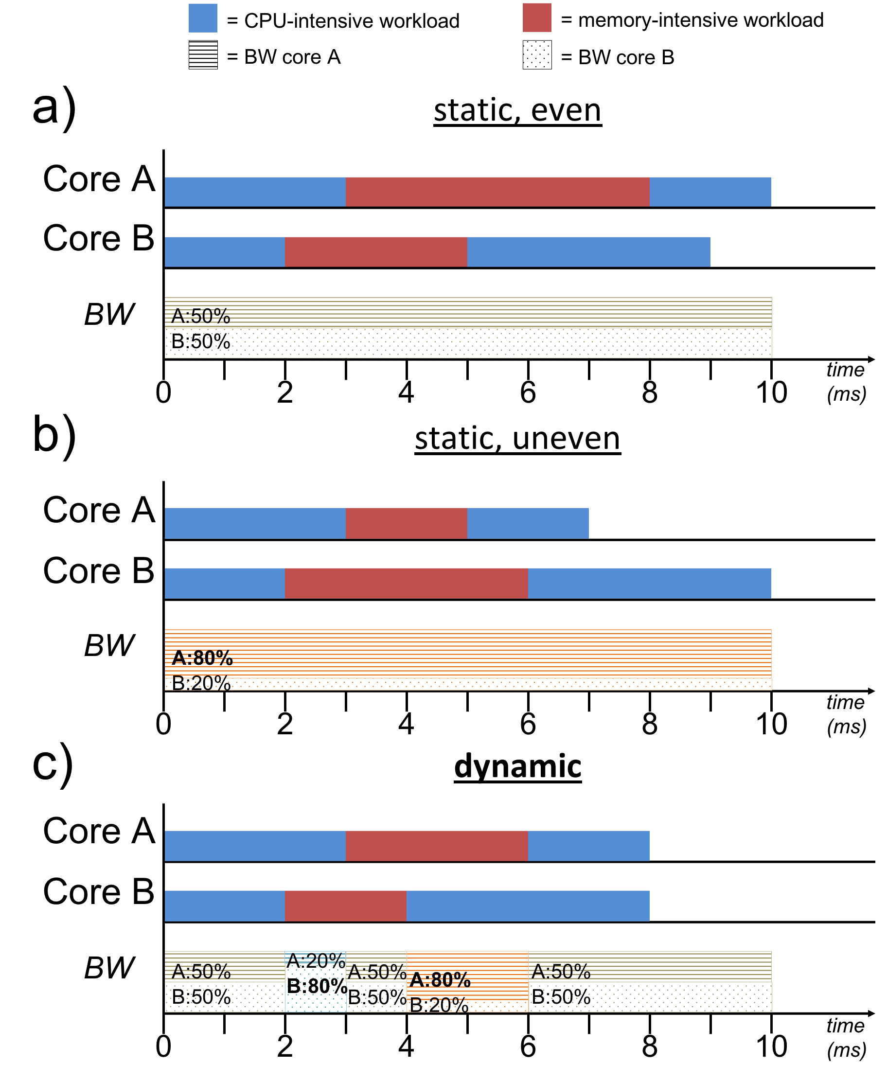
Figure 1: Example of static and even (a), static and uneven (b), and dynamic (c) memory bandwidth management on a 2-core (A and B) system.

In both uneven and even partitioning, memory bandwidth allocation is statically decided at design time, i.e., it does not change over time. The workload on each core, however, can undergo variations in terms of memory requirements. This is often the case as more/less memory-intensive tasks (or partitions) are scheduled on each core. As such, it is natural to consider a scheme where bandwidth-to-cores assignment is varied over time. In this case, we talk of dynamic bandwidth partitioning, i.e., memory scheduling. Figure 1 depicts one such example. Here, when only one core is executing memory-intensive workload, it is given 80% of the available bandwidth; when both are executing the same type of workload, the bandwidth is evenly distributed. Under the new scheme, the system operates at 80% utilization. In general, dynamic bandwidth assignment can yield significant performance improvement, because it is possible to produce an assignment scheme that follows the memory requirements of scheduled workload over time.

In the next sections, we address the problem of computing the time it takes in the worst-case to complete execution of workload that: (i) has known memory and CPU requirements; and (ii) spans over an arbitrary and known sequence of bandwidth assignments.

III System Model and Assumptions

We hereby discuss the assumptions considered in our work. We also provide the basic terminology and notation required to present our results.

Multi-core Model: in this work, we assume a homogeneous multi-core system with $m$ cores. We use the index $i$ to refer to any of the $m$ cores, i.e., $i\in\{1,\ldots,m\}$. We make no assumption on the cache hierarchy, as we focus on the behavior of tasks with respect to main memory accesses. We only assume that hits in last-level cache (LLC) do not generate main memory traffic. Main memory transactions have fixed size, typically one cache line, indicated with $L_{size}$. We assume that access to main memory is granted to cores/processors following a round-robin scheme. We assume that the time to perform a single memory transaction is bounded in the interval: $[L_{min},L_{max}]$. We do not require all memory transactions to be of a fixed size; but assume that, in the worst-case, all transactions have the maximum size. As an additional simplification, we assume no transaction parallelism, meaning that $L_{max}$ is also the maximum amount of interference that a given core can suffer due to an active memory transaction directed to a different core. No re-ordering of requests originated by different cores occurs in the system. This behavior can be achieved in a traditional COTS DRAM setup by assigning private memory banks to cores [3, 2, 4]. With private banking, the available DRAM banks are partitioned among the available $m$ cores. These assumptions make the considered model compatible with the work in [5, 6, 7].

Workload Model: we consider a partitioned system in which each task in a set of tasks is statically assigned to one of the $m$ cores [8]. Since our focus is on the behavior of workload in memory, we abstract away the details of each task and only consider the “load”, or “workload” in terms of CPU time and the number of memory transactions that need to be completed by a given deadline. The load can correspond to a single task instance, or to an entire busy-period. This is in line with the approach followed in [6, 7, 9]. Reasoning in terms of workload allows us to remain generic with respect to the exact task scheduling strategy used at the CPU. For instance, under preemptive rate-monotonic scheduling (RM), in order to analyze the schedulability of a task $\tau$, one would consider the deadline-constrained “load” comprised by the execution (CPU time and memory transactions) of one instance of $\tau$, as well as that of all the instances of interfering higher-priority tasks. The deadline of the workload will be the deadline of $\tau$.

Without loss of generality, we model deadline-constrained workload on a core $i$ under analysis using three parameters: $C_{i}$, $\mu_{i}$, and $D_{i}$. Here, $C_{i}$ represents the worst-case amount of time required for pure execution on the CPU (no memory). For ease of notation, we will always consider the worst-case execution time in slots of $L_{max}$ and indicate the latter with $E_{i}=\lceil\frac{C_{i}}{L_{max}}\rceil$. It must hold that $E_{i}>0$. Next, $\mu_{i}$ represents the worst-case number of main memory transactions [10] to be completed by the relative deadline $D_{i}$. We often use $\beta=E_{i}+\mu_{i}$ as a shorthand notation for the overall CPU and memory requirement of the workload under analysis. We assume that new workload is always released synchronously with respect to regulation periods, and scheduling decisions (on both CPU and memory) are taken at the boundaries of regulation periods.

Memory Bandwidth Regulation Model: in order to unevenly partition the memory bandwidth across cores, a budget-based memory bandwidth regulation scheme is used, such as MemGuard [11]. In this regulation scheme, per-core bandwidth regulators use hardware-implemented performance counters to monitor the number of memory transactions performed by each core over a period of time $P$. For this reason, $P$ takes the name of “regulation period”. Note that the number of memory transactions over $P$ is a measure of bandwidth. Since the maximum latency of a single memory transaction is $L_{max}$, then in the worst-case it is always possible to perform $Q=\frac{P}{L_{max}}$ memory transactions in $P$. Each core can then be assigned a different budget $q_{i}$, as long as $\sum_{i}q_{i}\leq Q$. However, in order to fully utilize the already constrained memory bandwidth, we consider the case $\sum_{i}q_{i}=Q$ without loss of generality. The budget assigned to all the $m$ cores forms a vector, namely $\mathcal{Q}=\{q_{1},\ldots,q_{m}\}$.

The key idea of memory bandwidth regulation is the following. A core $i$ is given a budget $q_{i}$, which represents the number of memory transactions that core $i$ is allowed to perform during a regulation period $P$. The budget is replenished to $q_{i}$ at time zero and at every instant $k\cdot P$, with $k\in\mathbb{N}$. During a regulation period, the core executes tasks normally, performing memory transactions as needed. A hardware performance counter monitors the number of memory transactions, decreasing the residual budget accordingly. If core $i$ depletes its budget $q_{i}$ before the next replenishment, core $i$ is stalled until the next replenishment. $P$ is a system-wide parameter which should be smaller than the minimum task period in the system. $P$ is often experimentally set to $1$ ms [11, 12].

Memory Schedule: in this paper, we assume that the memory schedule is known, or that a critical instant can be found on the bandwidth-to-core assignment rule, if an online memory scheduling rule is used. This opens a whole new set of questions that are out of the scope of this work: e.g. optimality, or existence of critical instants for memory schedulers. As depicted in Figure 1(c), a memory schedule $\mathcal{S}=\{B^{1},\ldots,B^{N}\}$ is a time-ordered sequence of $N$ memory budget assignment intervals $B^{j}$. Each $B^{j}$ is of the form $B^{j}=(\mathcal{Q}^{j},L^{j})$, where $\mathcal{Q}^{j}=\{q^{j}_{1},\ldots,q^{j}_{m}\}$ is the budget-to-cores assignment used in interval $j$, and $L^{j}$ is the length in regulation periods of interval $j$. For instance, the memory schedule in Figure 1(c) is $\mathcal{S}=\{(\mathcal{Q},2),(\mathcal{Q}^{\prime},1),(\mathcal{Q},1),(\mathcal{Q}^{\prime\prime},2),(\mathcal{Q},4)\}$.

Workload Span: the goal of this work is to compute the maximum number of regulation periods required to execute the workload under analysis to completion. This goes under the name of span, and is defined below.

Definition 1 (Span)

We define span as the number of regulation periods to entirely complete $E_{i}$ units of execution and $\mu_{i}$ memory transactions for the considered workload. The span is indicated throughout the paper with the symbol ${W_{i}}$.

The workload, however, may span throughout a number of different memory scheduling intervals $B^{1},\ldots,B^{N}$. While the total span is indicated with ${W_{i}}$, the span of the workload over each interval $B^{j}$ is indicated with ${W^{j}_{i}}$. It must hold that $\sum_{j=1}^{N}{W^{j}_{i}}={W_{i}}$.

Since the intervals have fixed length and are ordered, ${W^{1}_{i}}$ must be equal to either $L^{1}$ or ${W_{i}}$, whichever is shorter. Then assuming ${W_{i}}>L^{1}$, the span ${W^{2}_{i}}$ over interval $B^{2}$ must be equal to the minimum of $L^{2}$ and ${W_{i}}-L^{1}$. In general, noticing that $\sum^{j-1}_{k=1}L^{k}$ is the cumulative length of intervals preceding $B^{j}$, the execution over interval $B_{j}$ must thus be equal to:

$${W^{j}_{i}}=\max\Big{(}0,\min\big{(}L^{j},{W_{i}}-\sum^{j-1}_{k=1}L^{k}\big{)}\Big{)}.$$ (1)

IV Memory Stall

A fundamental concept is the notion of memory stall. In general, a memory request originating from the core $i$ under analysis can be “stalled” for two reasons. The first reason is that the hardware memory arbiter has prioritized one or more other cores over $i$ for access to the memory subsystem (memory interference). The second reason is that the core under analysis has exhausted its budget and is stalled until the beginning of the next regulation period.

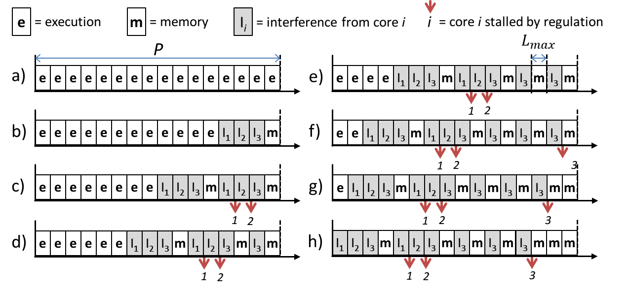
Figure 2: M/C configurations for core $i=4$ under analysis in a 4-core system with $\mathcal{Q}=\{2,2,5,7\}$.

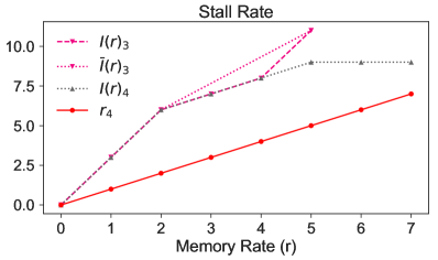
Figure 3: Plot of stall curves for a 4-core system with $\mathcal{Q}=\{2,2,5,7\}$.

We make no assumption on the behavior of tasks in cores other than core $i$. It follows that the maximum stall that can be suffered by a memory transaction on core $i$ depends only on the number of memory transactions performed by $i$ in the same regulation period. This is exemplified in Figure 3, where $i=4$ and $\mathcal{Q}=\{2,2,5,7\}$. The budget for Core 4 is $q_{4}=7$. It follows that there are 8 possible worst-case scenarios, denoted as (a)-(h) in the figure. In general, there are always $q_{i}+1$ possible cases. In the figure, pure execution is represented with “e” and is considered in slots of length $L_{max}$, as mentioned in Section III.

The pattern in Figure 3(a) depicts the worst-case memory interference from other cores (cores 1 to 3) provided that core 4 performs zero memory accesses within the regulation period. A more interesting case is Figure 3(e). Here, Core 4 performs 4 memory accesses. For the first two memory accesses, since three cores (1, 2 and 3) can cause stall, 3 units of stall are accumulated per memory access. If we depict the stall as a curve, then the “slope” of the stall introduced by the first two accesses is 3. After the first two accesses, cores 1 and 2 are temporarily stopped due to regulation – they have exhausted their respective budgets. Core 3, however, can still cause stall on transactions from Core 4 under analysis. Hence, the stall slope for the $3^{rd}$ and $4^{th}$ transactions is 1.

A more efficient way to visualize the possible stall scenarios is by plotting the per-period memory transactions and resulting stall. The $q_{i}+1$ possible cases represent a discrete domain. A corresponding continuous curve for the memory stall can be derived by “connecting” these discrete points. Call ${r_{i}}\in\mathbb{R}_{\geq 0}$ the number of memory transactions per regulation period being performed. We introduce the notion of memory rate.

Definition 2 (Memory rate)

We define as memory rate the number of memory transactions performed per regulation period. Memory rates are indicated throughout the paper with the symbol ${r_{i}}$.

A memory rate is often used to indicate the rate at which a total number of memory transactions $\mu_{i}$ is performed over the span of the considered workload ${W_{i}}$. Hence, $r_{i}=\frac{\mu_{i}}{{W_{i}}}$. We can also indicate the number of memory transactions performed during a specific interval $B^{j}$ as ${\mu^{j}_{i}}$. It must hold that $\sum_{j=1}^{N}{\mu^{j}_{i}}={\mu_{i}}$. Analogously, we indicate the memory rate over each interval as ${r^{j}_{i}}$. By definition, we have ${r^{j}_{i}}=\frac{{\mu^{j}_{i}}}{{W^{j}_{i}}}$.

IV-A Memory-stall Curves

The memory-stall curve for a core $i$ represents the cumulative maximum interference-induced stall for a given memory rate $r$ and is denoted as $I(r)_{i}$ . Consider same setup used for Figure 3. The memory-stall curves for cores 3 and 4 are provided in Figure 3. Considering Core 4, We have already discussed how the first two transactions introduce stall at a “slope” of 3. This is reflected in the $I(r)_{4}$ curve, since the curve has slope 3 when $r\in~{}]0,2[$.

For clarity, let us construct the memory-stall curve for core $3$. The $y$-axis represents the cumulative maximum stall $I(r)_{3}$ that can be experienced by workload on Core 3 with a memory rate $r$ ($x$-axis). Workload on Core 3 can perform of 0, 1, 2, 3, 4 or 5 memory transactions in a regulation period. The first step is to compute the maximum stall in each of these cases. If the workload does not perform any memory transaction ($r=0$) in a regulation period, then it will experience no stall, i.e. $I(0)_{3}=0$. When $r=1$, then it can be stalled by a maximum of $1$ memory transaction by each of the $m-1=3$ cores resulting in $I(1)_{3}=3$. Similarly, for all values of $r$ until $r=\min_{i}(q_{1},\ldots,q_{m})$, the maximum stall rate $I(r)_{3}=(m-1)\cdot r$, hence $I(2)_{3}=3\cdot 2=6$. When Core 3 performs an additional memory transaction, i.e. $r=3$, it can only be stalled by Core 4, since cores 1 and 2 have been regulated after their second memory access. Thus, the cumulative stall rate is $I(3)_{3}=I(2)_{3}+1\cdot 1=7$. Similarly, for $r=4$, $I(4)_{3}=I(3)_{3}+1\cdot 1=8$. Finally, for $r=5=q_{3}$, Core 3 is regulated. Here the maximum cumulative stall is $I(5)_{3}=Q-q_{3}=16-5=11$. The memory-stall curve $I(r)_{3}$ is obtained by connecting the discrete values of $I(k)_{3},k\in\{0,\ldots,5\}$ calculated so far.

Generalizing the example provided above, for any fixed budget $\mathcal{Q}$ we can define the stall curve $I(r)_{i}$ as follows:

$$I(r)_{i}=\begin{cases}\sum_{k\neq i}\min(r,q_{k})&\text{if}~{}r<q_{i}\\ Q-q_{i}&\text{if}~{}r=q_{i}\end{cases}$$ (2)

Since the budget assignment $\mathcal{Q}^{j}$ changes every scheduling interval $B^{j}$, a different $I(r)^{j}_{i}$ curve needs to be considered on each interval.

If the resulting curve is concave, then the memory-stall curve is already final. This is the case for $I(r)_{4}$ in Figure 3. Conversely, a refinement step is necessary to produce the final curve. Specifically, we take the upper-envelope of each of the convex segments to obtain a concave curve. The result of this step is depicted as $\bar{I}(r)_{3}$ in Figure 3.

Definition 3 (Stall rate)

We define as stall rate the amount of memory stall $\bar{I}(r)_{i}$ suffered per regulation period with a memory rate $r$. When considering multiple intervals, $\bar{I}(r)^{j}_{i}$ is the stall rate for core $i$ on interval $B^{j}$.

If the span over $B^{j}$ is ${W^{j}_{i}}$ and ${\mu^{j}_{i}}$ transactions are performed in the interval, we can compute the worst-case total stall ${S^{j}_{i}}$ over $B^{j}$ as:

$${S^{j}_{i}}:=\bar{I}({r^{j}_{i}})_{i}\cdot{W^{j}_{i}}=\bar{I}\Big{(}\frac{{\mu^{j}_{i}}}{{W^{j}_{i}}}\Big{)}_{i}\cdot{W^{j}_{i}}.$$ (3)

It follows that the total stall is ${S_{i}}=\sum_{j=1}^{N}{S^{j}_{i}}$. If the maximum memory stall that can be suffered by the workload under analysis can be derived, then the worst-case amount of time (in multiples of $L_{max}$) required to complete the considered workload is ${W_{i}}\cdot Q=\beta_{i}+{S_{i}}$. The rest of the paper is concerned with the calculation of the maximum total stall, and hence span, over a generic memory schedule $\mathcal{S}=\{B^{1},\ldots,B^{N}\}$.

For a fixed budget $\mathcal{Q}$, a given memory rate ${r_{i}}$ and span ${W_{i}}$, Lemma 1 guarantees that computing ${S_{i}}$ according to Equation 3 always results in an upper-bound on the maximum possible memory stall.

Lemma 1

${S_{i}}=\bar{I}({\mu_{i}}/{W_{i}})_{i}\cdot{W_{i}}$ is an upper bound to the cumulative stall suffered by a workload on core $i$ that performs ${\mu_{i}}$ memory accesses over ${W_{i}}$ regulation periods, with ${\mu_{i}}~{}\leq~{}{W_{i}}~{}\cdot q_{i}$.

Proof:

In each of the ${W_{i}}$ regulation periods, a number of memory accesses between $0$ and $q_{i}$ could have been performed; hence, note that we cannot have ${\mu_{i}}>{W_{i}}\cdot q_{i}$. Let us indicate with $a_{k}$ the number of periods in which $k$ memory accesses were performed. It must hold that $\sum^{q_{i}}_{k=0}a_{k}={W_{i}}$. We can then write:

$${\mu_{i}}=a_{0}\cdot 0+a_{1}\cdot 1+\ldots+a_{q_{i}}\cdot q_{i}.$$ (4)

The cumulative stall suffered over ${W_{i}}$ can be computed as:

$$a_{0}\cdot I(0)_{i}+a_{1}\cdot I(1)_{i}+\ldots+a_{q_{i}}\cdot I(q_{i})=\sum^{q_{i}}_{k=0}I(k)_{i}\cdot a_{k}.$$ (5)

Consider now computing the stall rate as $\bar{I}({\mu_{i}}/{W_{i}})_{i}$. From Equation 5, by $I(r)\leq\bar{I}(r)$ we have:

$$\sum^{q_{i}}_{k=0}I(k)_{i}\cdot a_{k}\leq\sum^{q_{i}}_{k=0}\bar{I}(k)_{i}\cdot a_{k}$$ (6)

Next recall that by definition of concavity for a generic function $f(x)$, it must hold that:

$$\lambda_{k}\in\mathbb{R}~{}~{}\text{s.t.}~{}\sum_{k}\lambda_{k}=1\implies f\Big{(}\sum_{k}x_{k}\lambda_{k}\Big{)}\geq\sum_{k}f(x_{k})\lambda_{k}$$ (7)

Note that:

$$\frac{\sum^{q_{i}}_{k=0}a_{k}}{{W_{i}}}=\sum^{q_{i}}_{k=0}\frac{a_{k}}{\sum^{q_{i}}_{k=0}a_{k}}=1.$$ (8)

Hence, we can write:

$$\footnotesize\frac{\sum^{q_{i}}_{k=0}\bar{I}(k)_{i}\cdot a_{k}}{{W_{i}}}=\sum^{q_{i}}_{k=0}\frac{\bar{I}(k)_{i}\cdot a_{k}}{\sum^{q_{i}}_{k=0}a_{k}}\leq\bar{I}\Bigg{(}\sum^{q_{i}}_{k=0}\frac{k\cdot a_{k}}{\sum^{q_{i}}_{k=0}a_{k}}\Bigg{)}_{i}=\bar{I}\Big{(}\frac{{\mu_{i}}}{{W_{i}}}\Big{)}_{i}.$$ (9)

This implies that $\bar{I}({\mu_{i}}/{W_{i}})_{i}\cdot{W_{i}}$ is an upper bound to the cumulative stall $\sum^{q_{i}}_{k=0}I(k)_{i}\cdot a_{k}$ suffered by the workload for any pattern of memory accesses over ${W_{i}}$ periods, concluding the proof. ∎

V WCET under Static Memory Budget

In this section, we present a fixed-point iterative algorithm to compute the worst-case length of the workload on a core under analysis $i$ under static memory budget $\mathcal{Q}$. This is useful to understand the basic mechanisms to compute the span over a generic single memory scheduling interval.

In each iteration, the algorithm recomputes the maximum stall and thereby, the workload span, based on the workload span from the previous iteration (except for the base iteration) and the corresponding memory schedule. The key intuition behind iterative recomputation is that the increase in workload span in an iteration is likely to increase the maximum stall in the consecutive iteration due to a different worst-case distribution of memory requests across (a) different per memory-stall curves and/or (b) different memory scheduling intervals.

In the rest of the paper, we will always focus on the generic core under analysis. As such, we will drop the index $i$ from all the notation introduced so far, unless required to resolve an ambiguity. Since we will be introducing a series of iterations of the algorithm, we subscript the iteration number (e.g., $(k)$) in the notation introduced so far.

Iterative Algorithm: the span $W$ over a static memory budget can be computed using Equation 10.

$${W_{(0)}} \leftarrow\lceil\beta/Q\rceil,$$

$${W_{(k)}} \leftarrow\Big{\lceil}\big{(}\beta+\bar{I}(\min({\mu}/{W_{(k-1)}}),q)\cdot{W_{(k-1)}}\big{)}/Q\Big{\rceil},$$ (10)

where the iteration continues until convergence with ${W_{(k)}}={W_{(k-1)}}$, or until ${W_{(k)}}\cdot Q\cdot L_{max}>D$. In the latter case, the workload in not schedulable. Since $\bar{I}(r)$ is only defined for $r\in[0,q]$, the term $\bar{I}(\min({\mu}/{W_{(k-1)}}),q)$ ensures that the function is never evaluated on a value outside its domain.

Theorem 1

The iteration in Equation 10 terminates in a finite number of steps by either obtaining a value ${W_{(k)}}\cdot Q\cdot L_{max}>D$, or by converging, in which case ${W_{(k)}}$ is an upper bound on the span of the workload on the core under analysis.

Proof:

Notice that we omit the proof for Theorem 1 here, as it is a corollary of the more general Theorem 2. As such, the proof is provided in the Appendix. ∎

For ease of explanation, Section 1 illustrates how to apply the algorithm in a specific instance. Subsequently, Section VI presents the generic algorithm.

Example of WCET over Static Budget: consider the static budget $\mathcal{Q}=\{2,2,5,7\}$. Let us now compute the span $W$ of the workload with $E=40$ and ${\mu}=35$ (i.e. $\beta=75$) executing on Core $3$. For simplicity, we ignore the workload’s deadline $D$ and focus only on its length. Since workload on Core $3$ is being analyzed, we consider the stall curve $\bar{I}(r)_{3}$ in Figure 3, with $Q=16$ and $q=5$.

The first step in the iterative Equation 10 is ${W_{(0)}}=\lceil\beta/Q\rceil=\lceil 75/16\rceil=5$. We then have:

$${W_{(1)}} =\lceil(75+\bar{I}(\min(35/5,5)\cdot 5)/16\rceil$$

$$=\lceil(75+\bar{I}(5)\cdot 5)/16\rceil=\lceil(75+11\cdot 5)/16\rceil=9$$

Since ${W_{0}}\neq{W_{k}}$, an additional iteration needs to be performed. We have:

$${W_{(2)}} =\lceil(75+\bar{I}(\min(35/9,5)\cdot 9)/16\rceil$$

$$=\lceil(75+\bar{I}(3.88)\cdot 9)/16\rceil=\lceil(75+9\cdot 9)/16\rceil=10$$

No convergence has been reached yet, so one more iteration is performed:

$${W_{(3)}} =\lceil(75+\bar{I}(\min(35/10,5)\cdot 10)/16\rceil$$

$$=\lceil(75+\bar{I}(3.5)\cdot 10)/16\rceil=\lceil(75+8.5\cdot 10)/16\rceil=10$$

Since ${W_{(3)}}={W_{(2)}}$, convergence has been reached and the worst-case length (in multiples of $L_{max}$) for the workload under analysis can be computed as ${W_{(3)}}\cdot Q=160$.

VI WCET under Dynamic Memory Budget

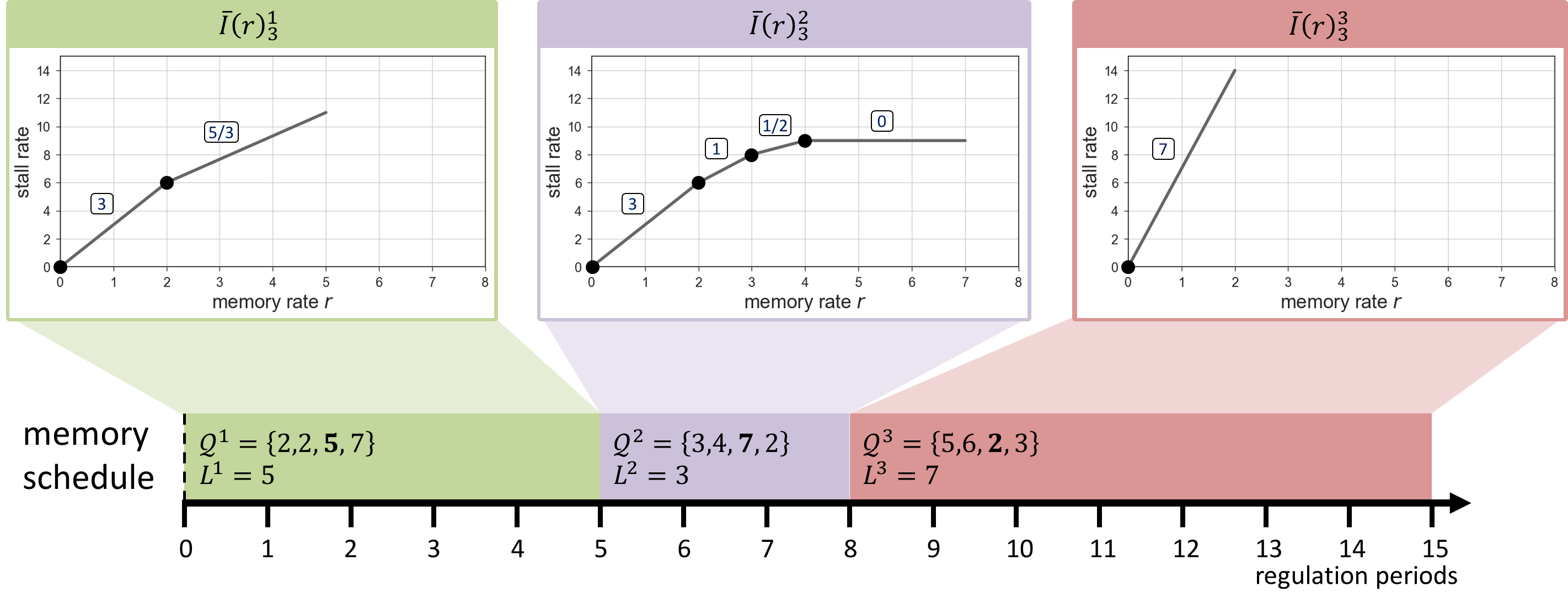
Figure 4: Example of memory schedule of length $15$ regulation periods composed of 3 intervals $B^{1},B^{2},B^{3}$ of length 5, 3, and 7, respectively. Considering Core 3, the curves $\bar{I}(r)^{1}_{3},\bar{I}(r)^{2}_{3},\bar{I}(r)^{3}_{3}$ are reported above each interval. For each $\bar{I}(r)^{j}_{3}$ curve, segment start points are highlights with a $\bullet$ and slopes are annotated above the segments.

In this section, we extend our analysis to the case of dynamic bandwidth assignment. In this case, the workload could span across one or more memory scheduling intervals $B^{1},\dots,B^{N}$. Recall from Section II that each interval $B^{j}=(\mathcal{Q}^{j},L^{j})$ is characterized by a budget-to-cores assignment $\mathcal{Q}^{j}=\{q^{j}_{1},\ldots,q^{j}_{m}\}$ and a length $L^{j}$ expressed in number of regulation periods. For the core under analysis, it is always possible to compute $\bar{I}(r)^{j}$ using Equation 2, i.e. the stall curve resulting from $\mathcal{Q}^{j}$.

Similarly to Equation 10, we follow an iterative approach. Let once again ${W_{(k)}}$ be the span of the considered workload at iteration $k$. It is always possible to determine the span of the workload ${W^{j}_{(k)}}$ in each of the intervals $B^{j}$ using Equation 1.

Example: To better understand this setup, consider the situation depicted in Figure 4. In this case, the memory schedule is composed of 3 intervals $B^{1},B^{2},B^{3}$. The intervals have length $L^{1}=5,L^{2}=3$, and $L^{3}=7$, respectively. Similarly we have three budget-to-cores assignments $\mathcal{Q}^{1},\mathcal{Q}^{2},\mathcal{Q}^{3}$ with the budgets values specified in the figure. Assume that we want to analyze the behavior of workload on Core $i=3$: the figure reports the $\bar{I}(r)^{1}_{3},\bar{I}(r)^{2}_{3},\bar{I}(r)^{3}_{3}$ curves that need to be considered in each of the intervals. Let us assume that at a certain iteration $k$, we have ${W_{(k)}}=9$ and apply Equation 1. We obtain ${W^{1}_{(k)}}=\max\big{(}0,\min(5,9)\big{)}=5,{W^{2}_{(k)}}=\max\big{(}0,\min(3,9-5)\big{)}=3$, and ${W^{3}_{(k)}}=\max\big{(}0,\min(7,9-8)\big{)}=1$. Note that it always hold $\sum_{j=1}^{N}{W^{j}_{(k)}}={W_{(k)}}$.

Assume that the span ${W_{(k)}}$ and hence the various ${W^{j}_{(k)}}$ terms at a given iteration $k$ are known. Then, the challenge is to determine how to distribute the total ${\mu}$ memory transactions among the $B^{1},\ldots,B^{N}$ intervals in a way that maximizes the overall stall. A distribution of memory transactions simply means that we derive the quantities ${\mu^{j}_{(k)}}$ for each $B^{j}$ interval. Obviously, it must hold that $\sum_{j=1}^{N}{\mu^{j}_{(k)}}={\mu}$. But among all the possible, valid distributions, we are interested in the one that maximizes the overall stall, i.e. ${S_{(k)}}=\sum_{j=1}^{N}{S^{j}_{(k)}}$, where each of the ${S^{j}_{(k)}}$ terms is defined as in Equation 3.

To simplify exposition, we first introduce an optimization problem in Algorithm 1 that computes the number ${\mu^{j}_{(k)}}$ of memory requests assigned to each interval $B^{j}$ at the $k$-th iteration to maximize the overall stall ${S_{(k)}}$. Then, in Section VI-B we show how to efficiently solve the optimization problem. Note that once ${\mu^{j}_{(k)}}$ has been determined, based on Lemma 1 the stall in interval $B^{j}$ can be upper-bounded as ${S^{j}_{(k)}}=\bar{I}({\mu^{j}_{(k)}}/{W^{j}_{(k)}})^{j}\cdot{W^{j}_{(k)}}$ . Hence, the cumulative stall at Line 8 of the algorithm is computed as ${S_{(k)}}=\sum_{j=1}^{N}{S^{j}_{(k)}}$. Due to regulation, in Line 12 we assign at most $q^{j}$ memory transactions in any regulation period inside interval $B^{j}$. This is equivalent to the following constraint: the number of transactions ${\mu^{j}_{(k)}}$ performed in $B^{j}$ is upper bounded by ${W^{j}_{(k)}}\cdot q^{j}$. Finally, since we know that the workload comprises at most $\mu$ requests, it must hold $\sum_{j=1}^{N}{\mu^{j}_{(k)}}\leq\mu$ at Line 13.

Based on Algorithm 1, ${W^{j}_{(k)}}$ is then computed according to the following iteration:

$${W_{(0)}} \leftarrow\lceil\beta/Q\rceil,$$

$${W_{(k)}} \leftarrow\Big{\lceil}\big{(}\beta+\sum_{j=1}^{N}\bar{I}({\mu^{j}_{(k-1)}}/{W^{j}_{(k-1)}})^{j}\cdot{W^{j}_{(k-1)}}\big{)}/Q\Big{\rceil}.$$ (11)

Note that at each iteration $k>0$, the values ${W^{j}_{(k-1)}}$ are computed using Equation 1 from ${W_{(k-1)}}$, and the values ${\mu^{j}_{(k-1)}}$ are computed using Algorithm 1. As in Section V, the iteration continues until convergence or ${W_{(k)}}\cdot Q\cdot L_{max}>D$.

Algorithm 1: Stall maximization over multiple intervals ⬇ 1Input: $B^{1},\ldots,B^{N}$ /* sequence of intervals */ 2Input: ${W^{1}_{(k)}},\ldots,{W^{N}_{(k)}}$ /* span in each interval */ 3Input: $\mu$ /* total memory requests */ 4 5Output: ${\mu^{1}_{(k)}},\ldots,{\mu^{N}_{(k)}}$ /* memory requests in each interval */ 6 7Maximize: /* max cumulative stall */ 8 ${S_{(k)}}=\sum_{j=1}^{N}{S^{j}_{(k)}}=\sum_{j=1}^{N}\bar{I}({\mu^{j}_{(k)}}/{W^{j}_{(k)}})^{j}\cdot{W^{j}_{(k)}}$ 9 10Subject to: 11 ${\mu^{j}_{(k)}}\in\mathbb{N}$ /* number of requests is natural */ 12 ${\mu^{j}_{(k)}}\leq{W^{j}_{(k)}}\cdot q^{j}$ /* max $q^{j}$ transactions per regulation period */ 13 $\sum_{j=1}^{N}{\mu^{j}_{(k)}}\leq\mu$ /* total requests constraint */

Example: Suppose we are analyzing the behavior of workload with $E=15$ and ${\mu}=25$ on Core 3 under the memory schedule depicted in Figure 4. Assume that at a given step $k$ we have ${W_{(k)}}=6$. In this case we have ${W^{1}_{(k)}}=5,{W^{2}_{(k)}}=1$ and ${W^{3}_{(k)}}=0$. Invoking Algorithm 1 returns the memory-to-intervals distribution that maximizes the overall stall, in this case: ${\mu^{1}_{(k)}}=22,{\mu^{2}_{(k)}}=3,{\mu^{3}_{(k)}}=0$. The stall per interval can be computed as ${S^{j}_{(k)}}=\bar{I}\big{(}{{\mu^{j}_{(k)}}/{W^{j}_{(k)}}}\big{)}\cdot{W^{j}_{(k)}}$. For this example, we have ${S^{1}_{(k)}}=50,{S^{2}_{(k)}}=8$ and ${S^{3}_{(k)}}=0$. The new value of ${W_{(k+1)}}$ can then be computed as ${W_{(k+1)}}=\lceil(35+50+8)/16\rceil=6$. Note that in this case Equation 11 has reached convergence.

VI-A Proof of Correctness

We now formally prove that Equation 11 computes a valid upper bound for the workload length in number of regulation periods. We begin with some helper lemmas; Lemma 2 show that the value of ${W_{(k)}}$ increases monotonically, which is required for the iteration to terminate, while Lemma 3 shows that if the iteration converges, we are able to distribute all $\mu$ memory requests among the $N$ memory scheduling intervals.

Lemma 2

At each iteration step in Equation 11 it holds: ${W_{(k)}}\geq{W_{(k-1)}}>0$.

Proof:

First note that functions $\bar{I}(r)^{j}$ are concave and $\bar{I}(0)^{j}=0$. For any such function and positive constant ${\mu}$, one can prove that $\bar{I}({\mu}/x)^{j}\cdot x$ is monotonic non-decreasing in $x>0$ (a formal proof is reported in Lemma 6 in Appendix). The proof then proceeds by induction over the index $k$.

Base Case: Since we assume $\beta>0$, we have ${W_{(0)}}>0$. Furthermore, since by definition all ${W^{j}_{(0)}}$ terms are non-negative and functions $\bar{I}(r)^{j}$ have non-negative ranges, $\sum_{j=1}^{N}\bar{I}({\mu^{j}_{(0)}}/{W^{j}_{(0)}})^{j}\cdot{W^{j}_{(0)}}$ is non-negative. By definition of Equation 11, this implies ${W_{(1)}}\geq{W_{(0)}}>0$.

Inductive Step: Consider $k\geq 2$. Note that in Equation 11, ${W_{(k)}}$ is computed based on the value of ${W_{(k-1)}}$, from which we obtain the values of ${W^{j}_{(k-1)}}$ in Equation 1 and ${\mu^{j}_{(k-1)}}$ in Algorithm 1; similarly, ${W_{(k-1)}}$ is computed based on ${W_{(k-2)}}$ and ${W^{j}_{(k-2)}},{\mu^{j}_{(k-2)}}$. By induction hypothesis, we have ${W_{(k-1)}}\geq{W_{(k-2)}}>0$; based on Equation 1, this implies ${W^{j}_{(k-1)}}\geq{W^{j}_{(k-2)}}$ for all intervals $B^{j}$.

Now consider Line 8 of Algorithm 1: since $\bar{I}(\mu/x)^{j}\cdot x$ is monotonic for $x>0$, it must hold:

$$\sum_{j=1}^{N}\bar{I}({\mu^{j}_{(k-2)}}/{W^{j}_{(k-1)}})^{j}\cdot{W^{j}_{(k-1)}}\geq$$

$$\sum_{j=1}^{N}\bar{I}({\mu^{j}_{(k-2)}}/{W^{j}_{(k-2)}})^{j}\cdot{W^{j}_{(k-2)}}.$$ (12)

In other words, when running Algorithm 1 at iteration $k$ based on the values ${W^{j}_{(k-1)}}$, there exists an assignment of variables (${\mu^{j}_{(k-1)}}={\mu^{j}_{(k-2)}}$, i.e., the same assignment as the previous iteration) that results in a value of the objective function that is greater than or equal to the one at iteration $k-1$. Furthermore, the assignment ${\mu^{j}_{(k-1)}}={\mu^{j}_{(k-2)}}$ is feasible, in the sense that it satisfies the constraints at Lines 11-13 of the algorithm: note that ${\mu^{j}_{(k-2)}}\leq{W^{j}_{(k-2)}}\cdot q^{j}$ implies ${\mu^{j}_{(k-1)}}\leq{W^{j}_{(k-1)}}\cdot q^{j}$ since ${W^{j}_{(k-1)}}\geq{W^{j}_{(k-2)}}$. Hence, given that the optimization problem is maximizing the objective function, it is guaranteed to find an assignment for variables ${\mu^{j}_{(k-1)}}$ such that:

$$\sum_{j=1}^{N}\bar{I}({\mu^{j}_{(k-1)}}/{W^{j}_{(k-1)}})^{j}\cdot{W^{j}_{(k-1)}}\geq$$

$$\sum_{j=1}^{N}\bar{I}({\mu^{j}_{(k-2)}}/{W^{j}_{(k-2)}})^{j}\cdot{W^{j}_{(k-2)}}.$$ (13)

In turn by definition of Equation 11 this implies ${W_{(k)}}\geq{W_{(k-1)}}$, concluding the induction step. ∎

Lemma 3

If the iteration in Equation 11 converges to a value ${W_{(k)}}$, then there exists a feasible assignment to variables ${\mu^{j}_{(k)}}$ that maximizes the objective function at Line 8 of Algorithm 1 and for which $\sum_{j=1}^{N}{\mu^{j}_{(k)}}=\mu$.

Proof:

Note that for a feasible assignment it cannot hold $\sum_{j=1}^{N}{\mu^{j}_{(k)}}>\mu$ due to the constraint at Line 13. Hence by contradiction, assume that for all assignments that maximize the objective function it holds: $\sum_{j=1}^{N}{\mu^{j}_{(k)}}<\mu$.

By definition, all ${W^{j}_{(k)}}$ terms are non negative. Furthermore, functions $\bar{I}(r)^{j}$ have non-negative ranges. Hence, increasing the value of a variable ${\mu^{j}_{(k)}}$ cannot cause the objective function to decrease. Therefore, $\sum_{j=1}^{N}{\mu^{j}_{(k)}}<\mu$ must hold even when each variable ${\mu^{j}_{(k)}}$ is assigned its maximum value, which is ${\mu^{j}_{(k)}}={W^{j}_{(k)}}\cdot q^{j}$ based on the constraint at Line 12. We thus obtain: $\sum_{j=1}^{N}{W^{j}_{(k)}}\cdot q^{j}<\mu$. Furthermore, note that we have $\bar{I}({\mu^{j}_{(k)}}/{W^{j}_{(k)}})^{j}=\bar{I}(q^{j})^{j}=Q-q^{j}$.

Finally, given $E>0$ and based on Equation 11 at convergence, we derive:

$${W_{(k)}} =\Big{\lceil}\big{(}\beta+\sum_{j=1}^{N}\bar{I}({\mu^{j}_{(k)}}/{W^{j}_{(k)}})^{j}\cdot{W^{j}_{(k)}}\big{)}/Q\Big{\rceil}$$

$$=\Big{\lceil}\big{(}E+\mu-\sum_{j=1}^{N}q^{j}\cdot{W^{j}_{(k)}}+\sum_{j=1}^{N}Q\cdot{W^{j}_{(k)}}\big{)}/Q\Big{\rceil}$$

$$>\Big{\lceil}\big{(}E+\sum_{j=1}^{N}(Q\cdot{W^{j}_{(k)}})\big{)}/Q\Big{\rceil}$$

$$=\lceil E/Q+{W_{(k)}}\rceil$$

$$\geq 1+{W_{(k)}},$$ (14)

which is a contradiction. ∎

Theorem 2

The iteration in Equation 11 terminates in a finite number of steps by either obtaining a value ${W_{(k)}}\cdot Q\cdot L_{max}>D$ or converging, in which case ${W_{(k)}}$ is an upper bound to worst-case span of the workload on the core under analysis.

Proof:

We first show that the algorithm terminates. By Lemma 2, ${W_{(k)}}\geq{W_{(k-1)}}$. Since ${W_{(k)}}$ is a natural number, it follows that the algorithm must either converge or terminate with a value of ${W_{(k)}}$ greater than the deadline in a finite number of steps.

Hence, assume that the algorithm converges to ${W_{(k)}}$. Based on Lemma 3, we can find an assignment to variables ${\mu^{j}_{(k)}}$ that maximizes the stall in the objective function of Algorithm 1 and such that $\sum_{j=1}^{N}{\mu^{j}_{(k)}}=\mu$. Hence, the assignment is valid, in the sense that the workload is able to perform its worst-case number of memory transactions. Furthermore, due to Line 12, it holds ${\mu^{j}_{(k)}}\leq{W^{j}_{(k)}}\cdot q^{j}$ for all intervals; hence, by Lemma 1 and for each $B^{j}$, ${S^{j}_{(k)}}=\bar{I}({\mu^{j}_{(k)}}/{W^{j}_{(k)}})^{j}\cdot{W^{j}_{(k)}}$ is an upper bound to the stall when performing ${\mu^{j}_{(k)}}$ memory accesses in ${W^{j}_{(k)}}$ regulation periods. Now given that Algorithm 1 maximizes the objective function at Line 8 over all possible assignments to variables ${\mu^{j}_{(k)}}$, it follows that $\sum_{j=1}^{N}{S^{j}_{(k)}}={S_{(k)}}$ is an upper bound to the cumulative stall when performing ${\mu}$ memory accesses over $\sum_{j=1}^{N}{W^{j}_{(k)}}={W_{(k)}}$ regulation periods.

Finally, by definition, the worst-case length of the workload can be obtained (in number of slots) as the sum of $\beta$ and the stall suffered by the workload. By convergence to ${W_{(k)}}$, we have:

$${W_{(k)}}\cdot Q=\Big{\lceil}\frac{{W_{(k)}}}{Q}\Big{\rceil}\cdot Q\geq\beta+\sum_{j=1}^{N}{S^{j}_{(k)}}=\beta+{S_{(k)}},$$ (15)

and since ${S_{(k)}}$ is an upper bound to the stall suffered in ${W_{(k)}}$ regulation periods, this implies that ${W_{(k)}}$ is indeed an upper bound to the total span of the workload. ∎

VI-B Implementing the Stall Algorithm

In this section, we show how to efficiently implement Algorithm 1. The algorithm is similar to a concave optimization problem, except that variables are integer rather than real.

By construction, each $\bar{I}(r)^{j}$ function is a concave piece-wise linear, and can be thought as a sequence of segments with decreasing slope. For each $\bar{I}(r)^{j}$ curve, consider the set of integer values of $r$ corresponding to the beginning of a segment. Call each of this values a start point, and ${\mathcal{E}^{j}}$ the set of all the start points in $\bar{I}(r)^{j}$. Start points are highlighted with a solid dot ($\bullet$) in Figure 4. Considering Core 3, for the example in the figure we have: ${\mathcal{E}^{1}}=\{0,2\},{\mathcal{E}^{2}}=\{0,2,3,4\}$, and ${\mathcal{E}^{3}}=\{0\}$.

Using this formulation, we introduce two helper functions defined on ${\mathcal{E}^{j}}$ for $\bar{I}(r)^{j}$. First, the ${\textrm{next}^{j}}(r)$ function returns the next start point strictly greater $r$:

$${\textrm{next}^{j}}(r):=\min_{p}\{p\in{\mathcal{E}^{j}}~{}|~{}p>r\}.$$ (16)

Second, the function ${\textrm{slope}^{j}}(r)$ simply returns the slope of the segment at $r$. If $r$ is a start point, the function returns the slope of the starting segment. Formally:

$${\textrm{slope}^{j}}(r):=\Big{(}\bar{I}\big{(}\textrm{next}^{j}(r)\big{)}^{j}-\bar{I}(r)^{j}\Big{)}/\big{(}\textrm{next}^{j}(r)-r\big{)}$$ (17)

All the slopes are annotated in Figure 4 right above the corresponding segment.

Algorithm 2 first initializes all variables ${\mu^{j}_{(k)}}$ to zero. Then, the algorithm iterates over Lines 9-19 until either (1) $\sum_{j=1}^{N}{\mu^{j}_{(k)}}=\mu$ holds, meaning that all $\mu$ memory transactions have been distributed among the $N$ memory scheduling interval; or (2) ${\mu^{j}_{(k)}}={W^{j}_{(k)}}\cdot q^{j}$ for all intervals, meaning that we cannot assign any more memory transactions due to the regulation constraints. When the condition ${\mu^{j}_{(k)}}={W^{j}_{(k)}}\cdot q^{j}$ holds for some interval $B^{j}$, we say that $B^{j}$ is saturated. The set of all the unsaturated intervals is computed at Line 11, and their respective memory rates $r^{j}$ given the current assignment ${\mu^{j}_{(k)}}$ is computed at Line 13.

For each iteration, at Line 15 the algorithm selects the interval $B^{j}$ with the highest slope for the currently assigned memory rate $r^{j}$ among all the unsaturated intervals – in case two intervals have the same slope, the tie can be broken arbitrarily. Finally, at Line 17 the value of memory transactions ${\mu^{p}_{(k)}}$ assigned to the selected interval $B^{p}$ is modified to the minimum of two expressions: (1) $\mu-\sum_{j\neq p}{\mu^{j}_{(k)}}$, that is, all remaining transactions. In this case, after the assignment, it holds that $\sum_{j=1}^{N}{\mu^{j}_{(k)}}=\mu$ and the algorithm terminates immediately. (2) ${\textrm{next}^{p}}(r^{p})\cdot{W^{p}_{(k)}}$, that is, ${\mu^{p}_{(k)}}$ is incremented so that $r^{p}={\mu^{p}_{(k)}}/{W^{p}_{(k)}}$ becomes equal to the next segment start point.

Algorithm 2: Stall maximization over multiple intervals ⬇ 1Input: $B^{1},\ldots,B^{N}$ /* sequence of intervals */ 2Input: ${W^{1}_{(k)}},\ldots,{W^{N}_{(k)}}$ /* span in each interval */ 3Input: $\mu$ /* total memory request */ 4 5Output: ${\mu^{1}_{(k)}},\ldots,{\mu^{N}_{(k)}}$ /* memory requests in each interval */ 6 7$\forall j:{\mu^{j}_{(k)}}$ $\leftarrow$ $0$ 8 9do: 10 /* consider only unsaturated intervals */ 11 $\mathcal{B}$ $\leftarrow$ $\{j~{}|~{}{\mu_{j}}(k)<{W^{j}_{(k)}}\cdot q^{j}\}$ 12 /* compute current memory rate $r$ on each unsaturated interval */ 13 $\forall j\in\mathcal{B}:r^{j}$ $\leftarrow$ ${\mu^{j}_{(k)}}/{W^{j}_{(k)}}$ 14 /* find curve $p$ where $r$ yields maximum stall slope */ 15 $p$ $\leftarrow$ $\textrm{argmax}_{j\in\mathcal{B}}\big{\{}{\textrm{slope}^{j}}(r^{j})\big{\}}$ 16 /* assign as many as possible transactions to this interval */ 17 ${\mu^{p}_{(k)}}$ $\leftarrow$ $\min\big{(}\mu-\sum_{j\neq p}{\mu^{j}_{(k)}},\textrm{next}^{p}(r^{p})\cdot{W^{p}_{(k)}}\big{)}$ 18 /* stop if all ${\mu}$ assigned, or all intervals are saturated */ 19until ($\sum_{j=1}^{N}{\mu^{j}_{(k)}}=\mu$ or $\forall j:{\mu^{j}_{(k)}}={W^{j}_{(k)}}\cdot q^{j}$)

Note that the segment start points, $\mu$ and ${W^{p}_{(k)}}$ are all natural numbers; hence, assuming that the values of variables ${\mu^{j}_{(k)}}$ were integer before the assignment at Line 15, the new value assigned to ${\mu^{p}_{(k)}}$ is also integer. Furthermore, the new assignment cannot violate the constraints $\sum_{j=1}^{N}{\mu^{j}_{(k)}}\leq\mu$ or ${\mu^{j}_{(k)}}\leq{W^{j}_{(k)}}\cdot q^{j}$, since we use the minimum of the two expressions. Hence, this shows that the assignment to variables ${\mu^{j}_{(k)}}$ operated by Algorithm 2 is feasible according to the constraints at Lines 11-13 of Algorithm 1. Furthermore, note that Algorithm 2 is guaranteed to terminate after the assignment at Line 17 selects the first expression, or after all intervals have been saturated. The number of segment start points for each function $\bar{I}(r)^{j}$ is $\mathcal{O}(m)$; hence, the number of iteration of the algorithm is $\mathcal{O}(N\cdot m)$.

Finally, we show that once the algorithm terminates, the assignment to variables ${\mu^{j}_{(k)}}$ maximizes the cumulative stall ${S_{(k)}}=\sum_{j=1}^{N}{S^{j}_{(k)}}=\sum_{j=1}^{N}\bar{I}({\mu^{j}_{(k)}}/{W^{j}_{(k)}})^{j}\cdot{W^{j}_{(k)}}$, that is, the objective function in Algorithm 1. This follows from the way intervals are selected at Line 15. By contradiction, assume that there exists a different feasible assignment, call it $\{\bar{\mu}^{1}_{(k)},\ldots,\bar{\mu}^{N}_{(k)}\}$, such that $\sum_{j=1}^{N}\bar{I}(\bar{\mu}^{j}_{(k)}/{W^{j}_{(k)}})^{j}\cdot{W^{j}_{(k)}}>\sum_{j=1}^{N}\bar{I}({\mu^{j}_{(k)}}/{W^{j}_{(k)}})^{j}\cdot{W^{j}_{(k)}}$; then can obtain $\{\bar{\mu}^{1}_{(k)},\ldots,\bar{\mu}^{N}_{(k)}\}$ by iteratively modifying $\{{\mu^{1}_{(k)}},\ldots,{\mu^{N}_{(k)}}\}$, subtracting some number of memory transactions, say $\Delta$, from one variable ${\mu^{j}_{(k)}}$ and adding them to another variable ${\mu^{p}_{(k)}}$. Now define:

$$\textrm{slope}^{p} =\frac{\bar{I}\big{(}({\mu^{p}_{(k)}}+\Delta)/{W^{p}_{(k)}}\big{)}^{p}-\bar{I}({\mu^{p}_{(k)}}/{W^{p}_{(k)}})^{p}}{\Delta/{W^{p}_{(k)}}},$$

$$\textrm{slope}^{j} =\frac{\bar{I}({\mu^{j}_{(k)}}/{W^{j}_{(k)}})^{j}-\bar{I}\big{(}({\mu^{j}_{(k)}}-\Delta)/{W^{j}_{(k)}}\big{)}^{j}}{\Delta/{W^{j}_{(k)}}},$$ (18)

as the resulting slopes for functions $\bar{I}(r)^{p}_{i}$ and $\bar{I}(r)^{j}_{i}$. Note that the modification to the variables will increase the cumulative stall by $\textrm{slope}^{p}\cdot\Delta$ and reduce it by $\textrm{slope}^{j}\cdot\Delta$. But because Line 15 always selects the function with the highest slope, it must be $\textrm{slope}^{p}\leq\textrm{slope}^{j}$; hence, the cumulative stall cannot increase, a contradiction. In summary, we have shown the following lemma:

Lemma 4

Algorithm 2 terminates in a finite number of steps. Furthermore, the resulting assignment to variables $\{{\mu^{1}_{(k)}},\ldots,{\mu^{N}_{(k)}}\}$ determines a value of $\sum_{j=1}^{N}\bar{I}({\mu^{j}_{(k)}}/{W^{j}_{(k)}})^{j}\cdot{W^{j}_{(k)}}$ equal to the value of the objective function computed by Algorithm 1.

Computational Complexity: note that each iteration of the algorithm can be easily optimized to execute in $\mathcal{O}(1)$. The sum of variables ${\mu^{j}_{(k)}}$ at Lines 17, 19 can be executed in constant time by keeping the sum in a variable and updating it each time ${\mu^{p}_{(k)}}$ is modified at Line 17. The selection at Line 15 can be performed in constant time by creating a table of segments ordered by slope. Since ordering the segments then dominates the complexity of the algorithm, this results in a $\mathcal{O}\big{(}N\cdot m\cdot\log(N\cdot m)\big{)}$ time for Algorithm 2. Note that, the analysis assumes a know memory schedule, but, is generic with respect to CPU scheduling. Thus, it is applicable to event-triggered CPU schedulers.

VII Scenario: Budget Assignment and Schedulability Ratios for IMA Partitions

Integrated Modular Avionics (IMA) systems use time-triggered scheduling of partitions, also known as ARINC 653 scheduling, where each partition is assigned, at compile time, a fixed start time and span in a major cycle i.e., a hyperperiod (H). These partition-level scheduling decisions are stored at compile time resulting in a static CPU schedule, which is repeated every major cycle.

Our analysis (Section VI) works with known memory assignment across cores and known workload parameters. IMA systems are a natural fit, representing a real-world scenario. We consider a set of IMA partitions with a fixed major cycle and assignment of partitions to cores. For simplicity, we assume the order of execution of the partitions is known, and we assume that each partition executes once in the major cycle, and that the major cycle is synchronized among cores. Our goal is to use our analysis from Section VI and perform an empirical evaluation comparing the ratio of schedulable tasksets to generated tasksets, under dynamic memory budget assignment policy against the static budget assignment policies, under a fixed partition execution order on each core.

In the next Subsections, we describe the setup used to compare the budget assignment policies and the two sets of experiments, one, that varies the number of cores and two, that varies the number of memory intensive partitions in a system.

VII-A Setup

IMA Partition Set Generation: For each experiment run, we consider $m$ cores and a set of $4\times m$ IMA partitions, with a fixed major cycle, i.e., hyperperiod (H) of $128ms$. The earliest start time of each partition is set to $t=0$ and the deadline to the hyperperiod i.e. $128ms$. From the perspective of the analysis (Section VI), each partition is a workload.

We characterize the varying memory demand between partitions as exhibited by avionic applications [13], using a parameter — memory intensity (MI) — , that represents the ratio of pure memory demand to the sum of pure processing demand and pure memory demand of a partition under single-core case i.e., no contentions. We then use a bi-modal distribution for $MI$, where each partition either has a HIGH MI mode or a LOW MI mode. The use of two modes is first, consistent with the memory intensity behavior exhibited by partitions in a real avionic application [13], and second, some partitions perform I/O activity that is memory- intensive. All HIGH MI mode partitions are randomly assigned an $MI$ value in the range of $[0.5,0.99]$, whereas for LOW MI mode partitions, the $MI$ value range is $[0.001,0.1]$. We use a parameter memory intensity ratio $MIr$ to vary the number of partitions in the HIGH MI mode to that in the LOW MI mode in the system.

Each partition is then randomly assigned a core, such that each core ends up with $4$ partitions. The setup then generates per partition single-core utilization using UUniFast algorithm [14] such that $U$ is the cumulative single-core utilization of each core. The parameter $U$ allows varying the cumulative single-core utilization of partitions assigned to a core. Next, the setup generates $E$ and $\mu$ values for each partition based on its single-core utilization and memory intensity (MI) value, assuming no stall. The $E$ and $\mu$ values of each partition respectively represent an aggregated $E$ demand and an aggregated $\mu$ demand of all tasks assigned to it, in line with existing works like [15] and [13].

System-wide Parameters: We use realistic system-wide parameters: $L_{max}=2.4\times 10^{-6}s$, $P=1ms$, resulting in $Q=41666$ as described in [6].

Budget Assignment Policies: We consider two static budget assignment policies: Static and even (SE) that assigns to each core a constant and identical budget of $1/m$ times the total budget, e.g., for a 4-core system $\mathcal{Q}=${10416, 10416, 10416, 10416}, and static and uneven (SU) that assigns to each core a constant budget based on the weight of each core, e.g., $\mathcal{Q}=\{416,20416,5416,15416\}$. For the SU policy, we use a heuristic to generate the weight of each core and thereby, a budget assignment, based on the input partition set.

The key idea behind the heuristic is to assign cores with higher memory demand a higher memory budget. The heuristic computes weight of each core based on the ratio of the remaining cumulative $\mu$ to that of the sum of remaining cumulative $\mu$ and cumulative $E$ on a core. Then, the memory bandwidth $Q$ is partitioned among cores based on the computed weights resulting in a budget assignment. This is similar to the term memory intensity, albeit on a core-level.

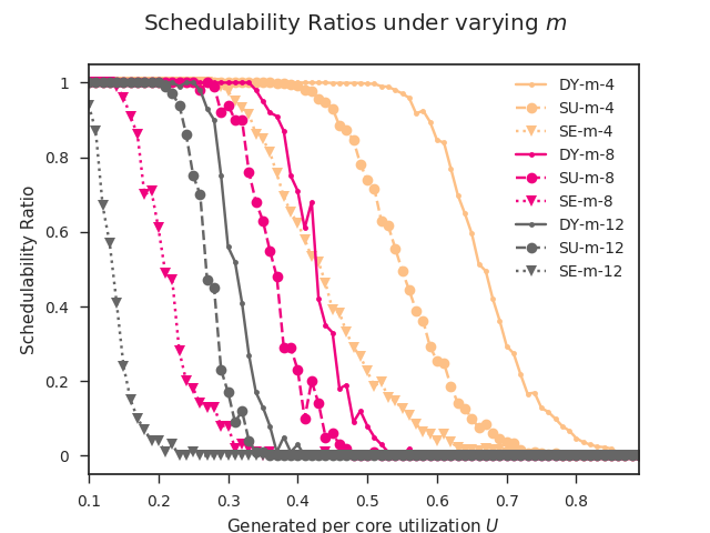
Figure 5: Schedulability ratios under varying $m$ from $4$ to $12$ cores in steps of $4$, for memory budget assignment policies: Dynamic (DY), Static Uneven (SU), and Static Even (SE). Memory intensity ratio $MIr$ of $0.25$

We compare the static policies (SE and SU) against a dynamic policy (DY), which assigns dynamic memory budgets to cores, using the heuristic. As compared to the static SU policy that uses the heuristic at time $t=0$ only, DY policy recomputes the weight of every core each time a partition finishes execution, resulting in a dynamic budget assignment.

VII-B Varying Number of Cores $m$

Figure 5 compares the schedulability ratios for each of the three budget assignment policies — DY, SU and SE —- under varying the number of cores $m$ from $4$ to $12$ in steps of $4$, for a fixed memory intensity ratio $MIr$ of $0.25$. In Figure 5, for each value of $U$, we generated $1000$ partition sets for $m=4$ case, and $100$ partition sets for each of $m=8$ and $m=12$ cases. On the x-axis, we vary the cumulative per core utilization $U$ from $0.1$ to $0.9$ in steps of $0.01$.

First, we observe that as the number of cores $m$ increases, the schedulability ratio decreases for the plots shift towards the left, for each of the three budget assignment policies. This is because, with increasing the number of cores, the total memory supply remains constant, albeit the total memory demand increases as the number of HIGH MI mode partitions increase in the system. Second, for each value of $m$, the dynamic policy DY dominates the static policies SU and SE.

VII-C Varying Memory Intensity ratio $MIr$

Now, we vary the memory intensity ratio $MIr$ from $0.15$ to $0.50$ that impacts the number of HIGH MI partitions in the system, and consequently, the number of LOW MI partitions in the system. We set the number of cores $m$ to $8$.

Figure 6 shows the schedulability ratios for each of the three budget assignment policies — DY, SU and SE —- under varying $MIr$. On the x-axis, we vary the cumulative per core utilization $U$ from $0.1$ to $0.9$ in steps of $0.01$. In Figure 6, we generated $100$ partition sets for every combination of $U$ and $MIr$.

As the $MIr$ ratio increases, the cumulative memory load from all cores on the memory increases, in general. Consequently, we observe that schedulability ratio plots shift towards the left on increasing the $MIr$ ratios. Further, for each memory intensity ratio $MIr$, the dynamic budget assignment policy DY dominates static policies SU and SE.

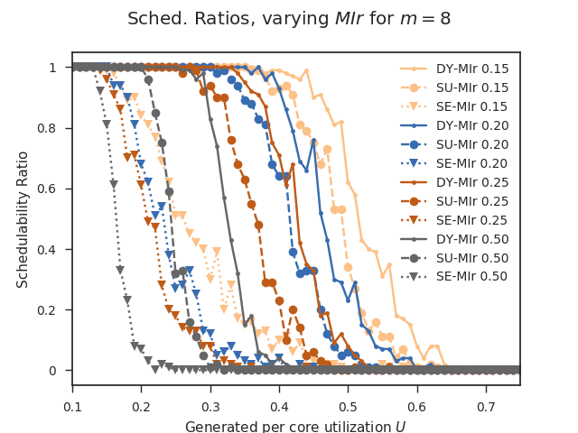
Figure 6: Schedulability ratios under varying memory intensity ratio $MIr$ from $0.15$ to $0.50$, for memory budget assignment policies: Dynamic (DY), Static Uneven (SU), and Static Even (SE). The number of cores $m$ is set to $8$.

VIII Related Work

Recent literature on the design of real-time systems on multi-core platforms considers main memory as a significant source of unpredictability, and an important interfering channel to mitigate. Predictable memory controllers have been proposed in [16, 17, 18]. OS-level techniques implementable on COTS hardware to regulate access of cores to main memory have been proposed and evaluated in [11, 1, 19, 20]. Yet another body of work has investigated the idea of strictly serializing access of cores to main memory. For instance, the work in [21] clusters memory operations in tasks via cache pre-fetching using compiler-level transformations, defining memory- and execution- phases. Then, a central scheduler only allows at most one memory-phase to be active at any point in time. A similar scheme was adopted in [22, 23, 24, 25] using DMAs instead of CPU-initiated pre-fetches and scratchpad memories. A recent work [26] proposes an analysis for co-running tasks contending for memory resources, i.e. with no explicit bandwidth partitioning.

By clustering and serializing access to shared memory, interference is avoided by design. Compared to this approach, regulation has the advantage of being entirely implementable at OS-level. For memory regulation techniques, analytic bounds for the temporal behavior of tasks was also derived [9, 6, 7, 27]. Similarly, the work in [28] derives runtime guarantees when both a CPU server and memory regulation are used. These works focus on static memory bandwidth partitioning.

With respect to static and even budget assignment, a first analysis was derived in [6]. In [9], an analysis for static and uneven bandwidth partitioning was performed assuming only knowledge of the memory budget $q_{i}$ for the core under analysis, and assuming arbitrary assignment to the other $m-1$ cores. More recently, the work in [7] demonstrated that by leveraging exact knowledge of each core’s budget $q_{i}$ it is possible to drastically reduce the pessimism of the analysis.

A few works [11, 1] proposed unused budget reclamation. However, no offline guarantees can be provided on the dynamic portion of the assigned budget. The work in [29] considers budget reclamation and derives WCET guarantees assuming full knowledge of the workload on all cores. In a more recent work, Nowotsch et al. [30, 15] consider avionics temporal partitions with pre-defined budget assignment. In this way, they are able to compute offline the WCET of application inside a partition, albeit the budget may vary at the boundaries of partitions. Finally, the work in [13] relaxes the strict single budget-to-partition assignment in [15] and allows different budgets being assigned to a partition offline, enabling dynamic budget assignment, from a set of design-time fixed budgets. By assuming that memory stall is pre-computed in each budget, the WCET computation problem is then be decomposed in (1) assigning “compatible” budgets across cores; and (2) minimizing the use of high-budget slots by the task under analysis.

What sets this work apart is the generality of the provided results. Unlike the aforementioned literature, we do not assume any specific budget re-assignment scheme. In fact, we provide a methodology that can be used to compute the worst-case runtime of a task given any dynamic budget-to-core assignment. To use our results, either exact knowledge of budget assignment over time is known; or a critical instant for memory budget re-assignments should be identified.

IX Conclusion

In this paper, we presented a methodology to analyze the worst-case execution time and schedulability of real-time workload under dynamic memory scheduling. We first introduced a simple iterative algorithm to compute the span of workload under static and uneven budget-to-core assignment. We then generalized the problem to consider a generic memory schedule and formulated the worst-case span analysis as a stall-maximization problem. Next, we demonstrated that the problem has strong similarities with concave optimization and proposed a low-complexity solution to determine the access pattern that maximizes the overall memory stall. As a use case, we considered an IMA setting where a subset of partitions run memory-intensive workload. In this scenario, dynamic memory scheduling outperformed traditional static bandwidth partitioning. The analysis assumes a known memory schedule. It is, however, generic with respect to CPU scheduling. Thus, it is applicable for event-triggered CPU schedulers. As a future work, we intend to study online bandwidth scheduling strategies for which a critical instant on decisions taken of both processor and memory can be identified.

Appendix A Appendix

Lemma 5

Consider a function $f:\mathbb{R}_{\geq 0}\rightarrow\mathbb{R}$ such that $f$ is concave and $f(0)=0$. Then $\forall a,b\in\mathbb{R}_{\geq 0}$ with $b>a$:

$$f(a)-a\cdot\frac{f(b)-f(a)}{b-a}\geq 0.$$ (19)

Proof:

By definition of concave function, $\forall x,y\in\mathbb{R}_{\geq 0}$ and $\alpha\in[0,1]$ it holds:

$$f\big{(}(1-\alpha)\cdot x+\alpha\cdot y\big{)}\geq(1-\alpha)\cdot f(x)+\alpha\cdot f(y).$$ (20)

Substituting $x=0,y=b$ and $\alpha=\frac{a}{b}$ in Equation 20 and given $f(0)=0$ we have:

$$f(a)\geq\Big{(}1-\frac{a}{b}\Big{)}\cdot f(0)+\frac{a}{b}\cdot f(b)=\frac{a}{b}\cdot f(b).$$ (21)

Finally, using Equation 21 we obtain:

$$f(a)-a\cdot\frac{f(b)-f(a)}{b-a}=$$

$$\frac{f(a)\cdot b-f(a)\cdot a-f(b)\cdot a+f(a)\cdot a}{b-a}=$$

$$\frac{f(a)\cdot b-f(b)\cdot a}{b-a}\geq$$

$$\frac{\frac{a}{b}\cdot f(b)\cdot b-f(b)\cdot a}{b-a}=0,$$ (22)

which yields the hypothesis. ∎

Lemma 6

Consider a function $g:\mathbb{R}_{\geq 0}\rightarrow\mathbb{R}$ such that $g$ is concave and $g(0)=0$. Then $\forall\mu\in\mathbb{R}_{\geq 0},\forall x\in\mathbb{R}_{>0}$: $x\cdot g(\mu/x)$ is monotonic non decreasing in $x$.

Proof:

We have to show that $\forall x_{1},x_{2}\in\mathbb{R}_{>0}$ with $x_{2}>x_{1}$:

$$x_{2}\cdot g(\mu/x_{2})\geq x_{1}\cdot g(\mu/x_{1}).$$ (23)

Let us define $K=\frac{g(\mu/x_{1})-g(\mu/x_{2})}{1/x_{1}-1/x_{2}}$. We first show that:

$$g(\mu/x_{2})-K/x_{2}\geq 0.$$ (24)

Define $f(y)=g(\mu\cdot y),a=1/x_{2},b=1/x_{1}$. Note that it holds $b>a>0,f(0)=g(\mu\cdot 0)=0$, and since $g$ is concave, $f$ is also concave. Then we obtain by substitution: $g(\mu/x_{2})-K/x_{2}=f(a)-a\cdot\frac{f(b)-f(a)}{b-a}$, which by Lemma 5 is greater than or equal to 0.

Finally, using Equation 24 we obtain:

$$x_{2}\cdot g(\mu/x_{2})=x_{2}\cdot\big{(}g(\mu/x_{2})-K/x_{2}\big{)}+K\geq$$

$$x_{1}\cdot\big{(}g(\mu/x_{2})-K/x_{2}\big{)}+K=$$

$$x_{1}\cdot\big{(}g(\mu/x_{2})-K/x_{2}+K/x_{1}\big{)}=$$

$$x_{1}\cdot\big{(}g(\mu/x_{2})+K\cdot(1/x_{1}-1/x_{2})\big{)}=$$

$$x1\cdot\big{(}g(\mu/x_{2})+g(\mu/x_{1})-g(\mu/x_{2})\big{)}=x_{1}\cdot g(\mu/x_{1}),$$ (25)

completing the proof. ∎

Proof:

We show that the iteration in Equation 10 is a special case of Equation 11, which implies that Theorem 1 follows as a corollary of Theorem 2. ${W_{(0)}}$ is computed in the same way, so we reason about the expression for ${W_{(k)}}$.

Note that the static budget scenario in Section V is equivalent to a dynamic scenario where there is only one memory scheduling interval $B^{1}$ of unbounded length. Hence, we have ${W^{1}_{(k-1)}}={W_{(k-1)}}$, and we can define $\bar{I}(r)=\bar{I}(r)^{1}$ and $q=q^{1}$ without loss of generality. The stall term in Equation 11 is thus equal to:

$$\sum_{j=1}^{N}\bar{I}({\mu^{j}_{(k-1)}}/{W^{j}_{(k-1)}})^{j}\cdot{W^{j}_{(k-1)}}=$$

$$\bar{I}({\mu^{1}_{(k-1)}}/{W_{(k-1)}})\cdot{W_{(k-1)}}.$$ (26)

Next, consider Algorithm 1; since there is only one variable ${\mu^{1}_{(k-1)}}$, the constraints at Lines 12, 13 are equivalent to: ${\mu^{1}_{(k-1)}}\leq{W_{(k-1)}}\cdot q$ and ${\mu^{1}_{(k-1)}}\leq\mu$. But since increasing the value of the variable cannot cause the objective function to decrease, it follows that the assignment ${\mu^{1}_{(k-1)}}=\min(\mu,{W_{(k-1)}}\cdot q)$ must maximize the stall. Substituting this value into Equation 26 yields:

$$\bar{I}\big{(}\min(\mu,{W_{(k-1)}}\cdot q)/{W_{(k-1)}}\big{)}\cdot{W_{(k-1)}}=$$

$$\bar{I}\big{(}\min(\mu/{W_{(k-1)}},q)\big{)}\cdot{W_{(k-1)}},$$ (27)

which is the stall term in Equation 10. This shows that the two iterations over ${W_{(k)}}$ are identical, completing the proof.

∎

References

- [1] H. Yun, G. Yao, R. Pellizzoni, M. Caccamo, and L. Sha, “Memory bandwidth management for efficient performance isolation in multi-core platforms,” IEEE Transactions on Computers, vol. 65, no. 2, pp. 562–576, Feb 2016.
- [2] H. Kim, D. de Niz, B. Andersson, M. Klein, O. Mutlu, and R. Rajkumar, “Bounding memory interference delay in cots-based multi-core systems,” in 2014 IEEE 19th Real-Time and Embedded Technology and Applications Symposium (RTAS), April 2014, pp. 145–154.
- [3] H. Yun, R. Mancuso, Z. P. Wu, and R. Pellizzoni, “Palloc: Dram bank-aware memory allocator for performance isolation on multicore platforms,” in 2014 IEEE 19th Real-Time and Embedded Technology and Applications Symposium (RTAS), April 2014, pp. 155–166.
- [4] R. Pellizzoni and H. Yun, “Memory servers for multicore systems,” in 2016 IEEE Real-Time and Embedded Technology and Applications Symposium (RTAS), April 2016, pp. 1–12.
- [5] L. Sha, M. Caccamo, R. Mancuso, J. E. Kim, M. K. Yoon, R. Pellizzoni, H. Yun, R. B. Kegley, D. R. Perlman, G. Arundale, and R. Bradford, “Real-time computing on multicore processors,” Computer, vol. 49, no. 9, pp. 69–77, Sept 2016.
- [6] R. Mancuso, R. Pellizzoni, M. Caccamo, L. Sha, and H. Yun, “Wcet(m) estimation in multi-core systems using single core equivalence,” in 2015 27th Euromicro Conference on Real-Time Systems, July 2015, pp. 174–183.
- [7] R. Mancuso, R. Pellizzoni, N. Tokcan, and M. Caccamo, “WCET derivation under single core equivalence with explicit memory budget assignment,” in 29th Euromicro Conference on Real-Time Systems, ECRTS 2017, June 27-30, 2017, Dubrovnik, Croatia, 2017, pp. 3:1–3:23. [Online]. Available: https://doi.org/10.4230/LIPIcs.ECRTS.2017.3
- [8] R. I. Davis and A. Burns, “A survey of hard real-time scheduling for multiprocessor systems,” ACM Comput. Surv., vol. 43, no. 4, pp. 35:1–35:44, Oct. 2011. [Online]. Available: http://doi.acm.org/10.1145/1978802.1978814
- [9] G. Yao, H. Yun, Z. P. Wu, R. Pellizzoni, M. Caccamo, and L. Sha, “Schedulability analysis for memory bandwidth regulated multicore real-time systems,” IEEE Transactions on Computers, vol. 65, no. 2, pp. 601–614, Feb 2016.
- [10] R. Mancuso, R. Dudko, E. Betti, M. Cesati, M. Caccamo, and R. Pellizzoni, “Real-time cache management framework for multi-core architectures,” in Proceedings of the IEEE Real-Time and Embedded Technology and Applications Symposium (RTAS), ser. RTAS’13. Philadelphia, PA, USA: IEEE Computer Society, April 2013, pp. 45–54.
- [11] H. Yun, G. Yao, R. Pellizzoni, M. Caccamo, and L. Sha, “MemGuard: Memory bandwidth reservation system for efficient performance isolation in multi-core platforms,” in Real-Time and Embedded Technology and Applications Symposium (RTAS), 2013, pp. 55–64.
- [12] ——, “Memory bandwidth management for efficient performance isolation in multi-core platforms,” IEEE Transactions on Computers, vol. 65, no. 2, pp. 562–576, Feb 2016.
- [13] A. Agrawal, G. Fohler, J. Freitag, J. Nowotsch, S. Uhrig, and M. Paulitsch, “Contention-Aware Dynamic Memory Bandwidth Isolation with Predictability in COTS Multicores: An Avionics Case Study,” in 29th Euromicro Conference on Real-Time Systems (ECRTS 2017), ser. Leibniz International Proceedings in Informatics (LIPIcs), M. Bertogna, Ed., vol. 76. Dagstuhl, Germany: Schloss Dagstuhl–Leibniz-Zentrum fuer Informatik, 2017, pp. 2:1–2:22. [Online]. Available: http://drops.dagstuhl.de/opus/volltexte/2017/7174
- [14] E. Bini and G. C. Buttazzo, “Measuring the performance of schedulability tests,” Real-Time Systems, vol. 30, no. 1, pp. 129–154, May 2005. [Online]. Available: https://doi.org/10.1007/s11241-005-0507-9
- [15] J. Nowotsch, M. Paulitsch, D. Buhler, H. Theiling, S. Wegener, and M. Schmidt, “Multi-core interference-sensitive wcet analysis leveraging runtime resource capacity enforcement,” in Real-Time Systems (ECRTS), 2014 26th Euromicro Conference on, July 2014, pp. 109–118.
- [16] D. Bui, E. Lee, I. Liu, H. Patel, and J. Reineke, “Temporal isolation on multiprocessing architectures,” in Design Automation Conference (DAC), June 2011, pp. 274 – 279.
- [17] B. Akesson, K. Goossens, and M. Ringhofer, “Predator: A predictable sdram memory controller,” in 2007 5th IEEE/ACM/IFIP International Conference on Hardware/Software Codesign and System Synthesis (CODES+ISSS), Sept 2007, pp. 251–256.
- [18] P. K. Valsan and H. Yun, “MEDUSA: A predictable and high-performance DRAM controller for multicore based embedded systems,” in 2015 IEEE 3rd International Conference on Cyber-Physical Systems, Networks, and Applications, Aug 2015, pp. 86–93.
- [19] J. L. Herman, C. J. Kenna, M. S. Mollison, J. H. Anderson, and D. M. Johnson, “RTOS support for multicore mixed-criticality systems,” in 2012 IEEE 18th Real Time and Embedded Technology and Applications Symposium, April 2012, pp. 197–208.
- [20] N. Kim, B. C. Ward, M. Chisholm, C. Y. Fu, J. H. Anderson, and F. D. Smith, “Attacking the one-out-of-m multicore problem by combining hardware management with mixed-criticality provisioning,” in 2016 IEEE Real-Time and Embedded Technology and Applications Symposium (RTAS), April 2016, pp. 1–12.
- [21] G. Yao, R. Pellizzoni, S. Bak, E. Betti, and M. Caccamo, “Memory-centric scheduling for multicore hard real-time systems,” in Real-Time Systems. Springer, 2011.
- [22] R. Tabish, R. Mancuso, S. Wasly, A. Alhammad, S. S. Phatak, R. Pellizzoni, and M. Caccamo, “A real-time scratchpad-centric OS for multi-core embedded systems,” in Real-Time and Embedded Technology and Applications Symposium (RTAS), 2016 IEEE 22th, April 2016.
- [23] S. Wasly and R. Pellizzoni, “A dynamic scratchpad memory unit for predictable real-time embedded systems,” in Real-Time Systems (ECRTS), 2013 25th Euromicro Conference on. IEEE, 2013, pp. 183–192.
- [24] M. R. Soliman and R. Pellizzoni, “WCET-Driven Dynamic Data Scratchpad Management With Compiler-Directed Prefetching,” in 29th Euromicro Conference on Real-Time Systems (ECRTS 2017), ser. Leibniz International Proceedings in Informatics (LIPIcs), M. Bertogna, Ed., vol. 76. Dagstuhl, Germany: Schloss Dagstuhl–Leibniz-Zentrum fuer Informatik, 2017, pp. 24:1–24:23. [Online]. Available: http://drops.dagstuhl.de/opus/volltexte/2017/7175
- [25] G. Durrieu, M. Faugère, S. Girbal, D. Gracia Pérez, C. Pagetti, and W. Puffitsch, “Predictable Flight Management System Implementation on a Multicore Processor,” in Embedded Real Time Software (ERTS’14), TOULOUSE, France, Feb. 2014. [Online]. Available: https://hal.archives-ouvertes.fr/hal-01121700
- [26] B. Andersson, H. Kim, D. D. Niz, M. Klein, R. R. Rajkumar, and J. Lehoczky, “Schedulability analysis of tasks with corunner-dependent execution times,” ACM Trans. Embed. Comput. Syst., vol. 17, no. 3, pp. 71:1–71:29, May 2018.
- [27] R. Pellizzoni and H. Yun, “Memory servers for multicore systems,” in 2016 IEEE Real-Time and Embedded Technology and Applications Symposium (RTAS), April 2016, pp. 1–12.
- [28] M. Behnam, R. Inam, T. Nolte, and M. Sjödin, “Multi-core composability in the face of memory-bus contention,” SIGBED Rev., vol. 10, no. 3, pp. 35–42, Oct. 2013. [Online]. Available: http://doi.acm.org/10.1145/2544350.2544354
- [29] J. Flodin, K. Lampka, and W. Yi, “Dynamic budgeting for settling DRAM contention of co-running hard and soft real-time tasks,” in Proceedings of the 9th IEEE International Symposium on Industrial Embedded Systems (SIES 2014), June 2014, pp. 151–159.
- [30] J. Nowotsch and M. Paulitsch, “Quality of service capabilities for hard real-time applications on multi-core processors,” in Proceedings of the 21st International Conference on Real-Time Networks and Systems, ser. RTNS ’13. New York, NY, USA: ACM, 2013, pp. 151–160.