Target Defense Against Link-Prediction-Based Attacks via Evolutionary Perturbations

Abstract

In social networks, by removing some target-sensitive links, privacy protection might be achieved. However, some hidden links can still be re-observed by link prediction methods on observable networks. In this paper, the conventional link prediction method named Resource Allocation Index (RA) is adopted for privacy attacks. Several defense methods are proposed, including heuristic and evolutionary approaches, to protect targeted links from RA attacks via evolutionary perturbations. This is the first time to study privacy protection on targeted links against link-prediction-based attacks. Some links are randomly selected from the network as targeted links for experimentation. The simulation results on six real-world networks demonstrate the superiority of the evolutionary perturbation approach for target defense against RA attacks. Moreover, transferring experiments show that, although the evolutionary perturbation approach is designed to against RA attacks, it is also effective against other link-prediction-based attacks.

1 Introduction

Many complex systems in the real world can be represented by networks, where the nodes denote the entities in the real systems and links capture various relationships among them [1, 2, 3, 4].

In network science, link prediction is a fundamental notion, which attempts to uncover missing links or to predict future interactions between pairwise nodes, based on observable links and other external information. Link prediction has various applications in many fields, e.g., link prediction itself can serve for network reconstruction [5], evaluating network evolving mechanism [6] and node classification [7]. Besides, in protein-protein interaction networks, link prediction can serve to guide the design of experiments to find previously undiscovered interactions [8]. With the boom of social media in recent years, service providers can leverage social networks and other information to recommend friends, commodities and advertisement that may attract users [9, 10, 11, 12, 13]. This process can also be naturally described as link prediction.

While various social media are enriching people’s lives [14, 15, 16], there is an increasing concern about privacy issues since more and more personal information could be obtained by others online. In the field of social privacy protection, many algorithms have been developed for protecting the privacy of users, such as identity, relationship and attributes, from different situations in which different public information was exposed to adversaries [17, 18, 19, 20]. In this paper, the focus is on preserving link privacy in social networks.

In retrospect, Zheleva et al. [20] proposed the concept of link re-identification attack, which refers to inferring sensitive relationships from anonymized network data. If the sensitive links can be identified by the released data, then this means privacy breach. In early days, link perturbation was considered a common technique to preserve sensitive links [21], e.g., a data publisher can randomly remove real links and insert fake links into an original network so as to preserve the sensitive links from being identified. Zheleva et al. [20] assumed that the adversary has an accurate probabilistic model for link prediction, and they proposed several heuristic approaches to anonymizing network data. Ying et al. [22] investigated the relationship between the level of link randomization and the possibility to infer the presence of a link in a network. Further, Ying et al. [23] investigated the effect of link randomization on protecting privacy of sensitive links, and they found that similarity indices can be utilized by adversaries to significantly improve the accuracy in predicting sensitive links.

Differing from the above approaches, Fard et al. [24] assumed that all links in a network are sensitive, and they proposed to apply subgraph-wise perturbations onto a directed network, which randomize the destination of a link within some subnetworks thereby limiting the link disclosure. Furthermore, they proposed neighborhood randomization to probabilistically randomize the destination of a link within a local neighborhood on a network [25]. It should be noted that both subnetwork-wise perturbation and neighborhood randomization perturb every link in the network based on a certain probability.

As discussed above, link prediction can be applied to predict the potential relationship between two individuals. From another perspective, it may also increase the risk of link disclosure. Even if the data owner removes sensitive links from the published network dataset, it may still be disclosed by link prediction and consequently lead to privacy breach. Michael et al. [26] presented a link reconstruction attack, which is a method that attacker can use link prediction to infer a user’s connections to others with high accuracy, but they did not mention how to defend the so-called link-reconstruction attack. Naturally, one can consider finding a way to prevent the link-prediction attack. Since link-reconstruction attack or link-prediction-based attack aims to find out some real but unobservable links, the defense of link-prediction-based attacks is also target-directed, which means that one has to preserve the targeted links from being predicted. In the literature, most existing approaches on link prediction are based on the similarity between pairwise nodes under the assumption that the more similar a pair of nodes are, the more likely a link exists between them.

In sociology, triadic closure is a popular concept to explain the evolution of a social network, i.e., if the triad of three individuals is not closed, then the person connected to the other two individuals would like to close this triad in order to achieve a closure in the relationship network [27]. Here, triadic closure breeds several neighborhood-based indices to measure the proximity of pairwise nodes. Zhou et al. [28] compared several neighborhood-based similarity indices on disparate networks, and they found that Resource Allocation (RA) index behaves best. Recently, Lü et al.  [29] published a survey on link prediction. In general, since many link prediction algorithms are designed based on network structures, a data owner can add perturbations into the original network to reduce the risk of targeted-link disclosure due to link-prediction-based attacks.

Note that, since a major goal of publishing social network data is to pursue useful and worthy research, one needs to limit the level of link perturbation. This reveals that the key of defending link-prediction-based attacks depends on how to find Optimal Link Perturbation (OLP), which takes the defense effect and the level of perturbation into account, to invalid link prediction algorithms, so that the removed sensitive links are hard to be correctly predicted. However, to the best of our knowledge, there are very few studies on this perspective of conducting target defense against link-prediction-based attacks. In this paper, the proposed approach is to randomly select some links as sensitive ones, assuming that the adversary employs the RA index to predict the missing links. Several approaches are proposed, including heuristic and evolutionary perturbations, to defend the attacks. It will be further shown that this kind of defense can also serve as a counterpart of link prediction to evaluate the robustness or vulnerability of various link prediction algorithms.

The main contributions of this paper are summarized as follows:

• A novel target defense method against link-prediction-based attacks is proposed to hide the sensitive links from being predicted.

• Techniques using heuristic as well as evolutionary perturbations to defend link-prediction-based attacks are developed. With evolutionary perturbations, a new fitness function is designed, taking into consideration of both precision and AUC (area under curve), which can reduce the calculation of fitness values by computing the variation after perturbations. The experimental results demonstrate the superiority of evolutionary perturbations, especially using an EDA (estimation of distribution algorithm), and it is found that the transfer effect is closely related to the fitness.

The rest of the paper is organized as follows. In Sec. 2, the network model and some standard metrics about link prediction are introduced. The proposed target defense against link-prediction-based attacks is discussed. In Sec. 3, several methods are developed, including heuristic and evolutionary perturbations. In Sec. 4, empirical experiments are conducted to examine the proposed methods, and the experimental results are analyzed in detail. In Sec. 5, the paper is concluded with some discussions on future directions of research.

2 Network model and performance metrics

2.1 Network Model

An undirected network is presented by $G(V,E)$, where $V$ and $E$ denote the sets of nodes and links, respectively. Define the set of all node pairs in the network by $\Omega=\{(i,j)|\{i,j\}\in V,i\neq j\}$. In an undirected network, link $(i,j)$ is considered the same as link $(j,i)$ and $\Omega$ contains $\binom{k}{2}=\frac{{|V|\left({|V|-1}\right)}}{2}$ possible links. All observable links $E$ are divided into two groups: the training set $E^{T}$ and the validation set $E^{V}$, where $E^{T}\cup E^{V}=E$ and $E^{T}\cap E^{V}=\emptyset$. Furthermore, define the set of unknown node pairs and the set of non-existent node pairs by ${U}=\Omega-{E^{T}}$ and ${N}=\Omega-E$, respectively. Obviously, ${U}={N}+E^{V}$.

2.2 Link Prediction

In link prediction, the objective is to predict $E^{V}$ within $U$ utilizing the structure information provided by $E^{T}$. There are several metrics to measure the similarity of node pairs, among which local indices are computationally efficient and well-performed. According to [28] and [30], the RA index stands out from several local similarity-based indices. It is defined as follows:

$$RA_{xy}=\sum\limits_{z\in\Gamma\left(x\right)\cap\Gamma\left(y\right)}{\frac{1}{{{d_{z}}}}}\,,$$ (1)

where $\Gamma(x)$ denotes the one-hop neighbors of node $x$ and $d_{z}$ denotes the degree of node $z$. To reduce the RA value of a certain node pair, one can decrease the number of common neighbors between them or increase the degree of their common neighbors.

In this paper, two standard metrics are used for measuring the performance of link prediction, i.e., precision and AUC (the area under the receiver operating characteristic curve), which are defined as follows:

• Precision
  Precision is the ratio of real missing links to predicted links. To calculate it, first sort node pairs in $U$ in descending order according to their similarity values, as $\hat{U}$, and then the top-$k$ node pairs ${\hat{U}}^{k}$ in ${\hat{U}}$ are chosen as the predicted ones. The definition of precision is

  $$precision=\frac{|{\hat{U}}^{k}\cap E^{V}|}{|E^{V}|}\,,$$ (2)

  where $k=|E^{V}|$ will be used in this paper.

• AUC
  AUC measures the probability that a random missing link in $E^{V}$ is given a higher similarity value than a random non-existent node pair in ${N}$. To calculate it, choose each missing link in $E^{V}$ and each non-existent link in ${N}$ to compare their values: if there are $n_{>}$ times where a missing link has a higher value and $n_{=}$ times their values are the same, then the AUC is computed as follows:

  $$AUC=\frac{n_{>}+0.5n_{=}}{n}\,,$$ (3)

  where $n=|E^{V}|*|{N}|$ will be used in this paper.

2.3 Target Defense in Link Prediction Attack

A new target defense method is proposed here against link-prediction-based attacks. For instance, as shown in Fig. 1, simply deleting the sensitive link $(i,j)$ cannot make it hidden, because the value of $RA_{ij}$ is equal to 1, which is much higher than other node pairs in the network. The deleted link could be easily re-identified, if RA is employed to predict missing links. However, if one deletes link $(i,q)$ and meanwhile inserts link $(p,q)$, then $RA_{ij}=0.5$, which is similar to other node pairs.

Figure 1: The whole process of defending link-prediction-based attacks via link perturbations. Red link $(i,j)$ is sensitive, which needs to be hidden, and green dashed link $(p,q)$ is the inserted link. The released network can preserve the sensitive link $(i,j)$ from being identified by the RA index, to some extent.

In a network $G(V,E)$, the set $E$ is divided into two disjoint groups: $E^{T}$ and $E^{V}$. Take $E^{V}$ as the set of sensitive links. The set of link perturbations $\tilde{E}$ is added into $E^{T}$, which means deleting $E_{del}$ from $E^{T}$ and then inserting $E_{add}$ into $E^{T}$ so as to reduce the rate that links in the set of sensitive links being re-identified by a link prediction algorithm $\mathcal{L}$, which consequently leads to the risk of privacy leakage.

Although the defensive effect may be improved as the number of modified links increases, the number of modifications should be minimized, taking into account the cost of perturbations and the utility of the perturbed network. Therefore, the following two restricted conditions are considered:

• the numbers of deleted and inserted links should be identical to make the total number of links unchanged.

• the numbers of deleted and inserted links should be sparse to ensure data utility.

Ut supra, target defense against link-prediction-based attacks can be described mathematically as follows:

$$\mathop{\textbf{min}}\limits_{\tilde{E}}\,\,\,\,\mathcal{L}(E^{T}+{\tilde{E}},E^{V})$$ (4)

$$\textbf{ s.t.}\quad\begin{cases}|\tilde{E}|=|E_{add}|+|E_{del}|=2\cdot|E_{del}|\ll|E^{T}|\\ E_{del}\subset E^{T},\,\,\,\,E_{add}\subset N\,.\end{cases}$$

After being perturbed, $E^{T}$, $U$ and $N$ of the original network are changed to $\tilde{E}^{T}$, $\tilde{U}$ and $\tilde{N}$, respectively. It then follows that

$${\tilde{E}^{T}} =E^{T}-E_{del}+E_{add},$$ (5)

$${\tilde{U}} =\Omega-(E^{T}+\tilde{E})=U+E_{del}-E_{add},$$ (6)

$${\tilde{N}} =\Omega-(E^{T}+\tilde{E})-E^{V}=N+E_{del}-E_{add}\,.$$ (7)

The relationship of each link set after a perturbation is shown in Fig. 2, where the set of non-existent node pairs before and after the perturbation are shown in grey.

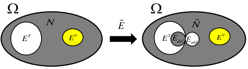
Figure 2: The venn diagram of each node-pair set after adding perturbation $\tilde{E}$ into the original network.

3 Methods

In this paper, assume that the adversary uses the RA index to predict the missing links. The objective here is to preserve $E^{V}$ from being predicted via adding link perturbations. Then, random, heuristic and evolutionary perturbations are applied, respectively, as discussed below.

3.1 Random Perturbations

3.1.1 Randomly Link Rewiring (RLR)

For a given network in which sensitive links are removed, one can randomly delete some links $\ell_{del}$ from $E^{T}$ and then insert the same number of new links $\ell_{add}$, which exist in $N$.

3.1.2 Randomly Link Swapping (RLS)

Another common practice for randomizing a network is link swapping, which not only keeps the total number of links unchanged but also preserves the degrees of nodes [31]. As shown in Fig. 3, link swapping removes two randomly chosen links from $E^{T}$ and creates two new links existing in $N$ before swapping.

Figure 3: An example for link swapping. If either $(i,v)$ or $(i,v)$ already exists in $E^{T}$, no swapping is performed, and another attempt is made to find a suitable link pair.

3.2 Heuristic Perturbation

To hide the links in $E^{V}$, one can degrade the performance of link prediction through decreasing the similarity values of node pairs in $E^{V}$ and then increasing the values of non-existent node pairs. Here, a greedy strategy is adopted to rewire links. First, the RA index is used to calculate the similarity values of node pairs $(i,j)\in\Omega$ and then sort them in descending order according to their values.

For each node pair $(i,j)\in\Omega$, there are three cases, i.e., $(i,j)\in E^{T}$, $(i,j)\in N$, and $(i,j)\in E^{V}$. One can traverse the ordered node pairs and conduct different operations by deleting or inserting links for each case.

• $(i,j)\in E^{T}$

  If the current node pair $(i,j)$ exists in $E^{T}$, directly delete the link. Because the deleted $(i,j)$ will exist in $\tilde{U}$ and $(i,j)$ has a high RA value.

• $(i,j)\in N$

  If the current node pair $(i,j)$ exists in $N$, select the node $k$ whose degree is the smallest in the one-hop neighborhoods of $i$ and $j$, except their common neighbors. Then, insert $(i,k)$ or $(j,k)$ to increase the RA value of the current node pair $(i,j)$.

• $(i,j)\in E^{V}$

  If the current node pair $(i,j)$ exists in $E^{V}$, select the common neighbor $k$ whose degree is the smallest and then delete $(i,k)$ or $(j,k)$; or select two common neighbors $k$ and $l$ whose degrees are among the smallest. Then, insert $(k,l)$ to reduce the RA value of the node pair $(i,j)$.

The above operation is shown in Fig. 4.

It should ensure that all deleted links $\ell_{del}\in E^{V}$ and inserted links $\ell_{add}\in N$. The intact pseudo-codes of the algorithms are described in Algorithms  1,  2 and  3.

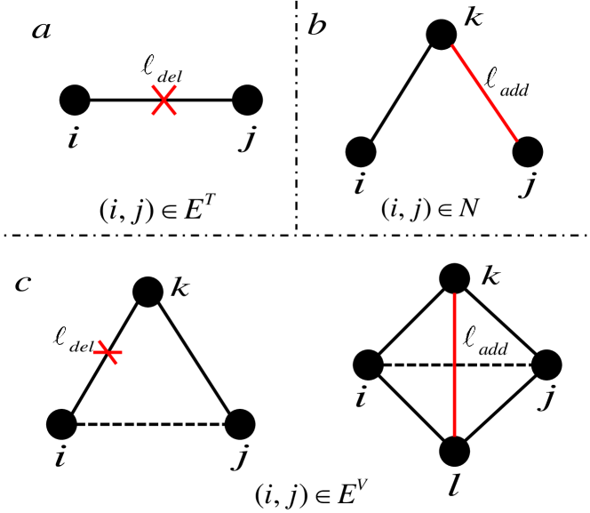
Figure 4: Four different operations through deleting or inserting links for $(i,j)$ in corresponding situations.

Input: $E^{T}$, $E^{V}$, N, $\Omega$ and $m$.

Output: $E_{del}$ and $E_{add}$.

1 Initialize $E_{del}$ and $E_{add}$;

2 sort $\Omega$ in descending order to get $\hat{\Omega}$;

3 for each $(i,j)\in\hat{\Omega}$ do

4       if $(i,j)\in E^{T}\cup E^{V}$ then

5             if $|E_{del}|<m$ then

6                  $\ell_{del}$ = Delete Link($(i,j)$);

7                   $E_{del}$ = $E_{del}\cup\ell_{del}$ ;

8                   continue;

9                  

10             end if

11            

12       end if

13       if $(i,j)\in E^{V}\cup N$ then

14            if $|E_{add}|<m$  then

15                  $\ell_{add}$ = Add Link($(i,j)$);

16                   $E_{add}$ = $E_{add}\cup\ell_{add}$;

17             end if

18            

19       end if

20       if $|E_{del}|=m$ and $|E_{add}|=m$  then

21            Break;

22       end if

23      

24 end for

return $E_{del}$ and $E_{add}$.

Algorithm 1 Heuristic Perturbation (HP)

Input: node pair $(i,j)$

Output: $\ell_{del}$

1 if $(i,j)\in E^{T}$ then

2       $E^{T}=E^{T}-(i,j)$;

3       return $(i,j)$;

4      

5 end if

6if $(i,j)\in E^{V}$ then

7      Find $k=\mathop{\arg\min}\limits_{k}\{d_{k}|k\in\Gamma\left(i\right)\cap\Gamma\left(j\right)\}$;

8       Find $l=\mathop{\arg\max}\limits_{l}\{{d_{l}}|l\in\{i,j\}\}$;

9       if $(k,l)$ exists then

10             $E^{T}=E^{T}-(k,l)$ ;

11             return $(k,l)$;

12            

13       end if

14      

15 end if

Algorithm 2 Delete Link

Input: node pair $(i,j)$

Output: $\ell_{add}$

1

2if $(i,j)\in E^{V}$ then

3       Find $k=\mathop{\arg\min}\limits_{k}\{d_{k}|k\in\Gamma\left(i\right)\cap\Gamma\left(j\right)\}$;

4       Find $l=\mathop{\arg\min}\limits_{l}\{d_{l}|l\in\{\Gamma\left(i\right)\cap\Gamma\left(j\right)-k\}\}$;

5       if $(k,l)$ exists and $(k,l)\notin E^{V}$ then

6             $E^{T}$ = $E^{T}\cup(k,l)$;

7             return $(k,l)$;

8            

9       end if

10      

11 end if

12if $(i,j)\in N$ then

13      Find $k=$ $\mathop{\arg\min}\limits_{k}\{d_{k}|k\in\{\Gamma\left(i\right)\cup\Gamma\left(j\right)-\Gamma\left(i\right)\cap\Gamma\left(j\right)\}\}$;

14       if $k$ exists then

15             $E^{T}$ = $E^{T}\cup\{(k,l)|(k,l)\notin E^{V},l\in\{i,j\}\}$;

16             return $\{(k,l)|(k,l)\notin E^{V},l\in\{i,j\}\}$;

17            

18       end if

19      

20 end if

Algorithm 3 Add Link

3.3 Evolutionary Perturbations

Link perturbation can be treated as a combinatorial optimization problem and the number of candidate combinations of deleted/inserted links is $C_{|E^{T}|}^{m}\cdot C_{|N|}^{m}$, where $m$ is the number of deleted/inserted links.

To hide sensitive links in $E^{V}$, one needs to reduce the possibility that these links can be predicted. Both AUC and precision are indicators for evaluating the performance of a link prediction algorithm. AUC evaluates the global performance while precision focuses on pairs with highest similarity values. Therefore, an evolutionary algorithm is designed here to find OLP, considering both AUC and precision together as the reduction objective.

Next, consider two evolutionary algorithms, i.e. Genetic Algorithm (GA) and Estimation of Distribution Algorithm (EDA). First, design the common chromosome, fitness and selection operation.

• Chromosome

  The chromosome consists of two parts: $\ell_{del}^{i}\in E^{T}$ and $\ell_{add}^{i}\in N$, $i=1,2,...,m$. The number of deleted and inserted links are identical according to the assumption. The diagram of chromosome is shown in Fig. 5, where the length of chromosome depends on the experimental setup.

• Fitness

  Two major link prediction performance measures, i.e. precision and AUC, are considered in the fitness design. Note that directly taking both precision and AUC as fitness is time-consuming. Thus, a new fitness function is designed to simplify the calculation, as follows:

  $$\mathop{\textbf{\emph{{max}}}}\limits_{\ell\in{E^{V}},n\in\tilde{N}} Fitness=\alpha\cdot{\sum\limits_{n\in\tilde{N}}{\delta(R{A_{n}}>\mathop{\max}\limits_{\ell\in{E^{V}}}\{R{A_{\ell}}\})}}$$ (8)

  $$+(\frac{1}{{|\tilde{N}|}}\sum\limits_{n\in\tilde{N}}{R{A_{n}}}-\frac{1}{{|{E^{V}}|}}\sum\limits_{\ell\in{E^{V}}}{R{A_{\ell}}})\,,$$

  where $\delta(x)$ is an indicator function: $\delta(x)=1$ when $x$ is true; otherwise, $\delta(x)=0$, and $\alpha$ is a tunable parameter. The fitness function consists of two parts: (1) denoting the number of non-existent links with higher similarity values than the most predictable sensitive pairs, which has greater influence on the precision; (2) denoting the difference in the average similarity values between non-existent pairs and sensitive pairs, which affects the AUC more.

  

  Figure 5: The diagram of chromosome in GA and EDA, respectively. It consists of two parts, i.e. deleted links $\ell_{del}\in E^{T}$ and inserted links $\ell_{add}\in N$.

• Selection Operation

  The selection operation is conducted on roulette. To make the fitness values positive, apply exponential transform $(e^{x})$ to the fitness. At the same time, retain $n_{elite}$ elites according to the fitness values.

• Mutation Operation

  Select $n_{mutation}$ chromosomes based on the fitness values for mutation operation. Then, traverse each link in a chromosome and conduct mutation operation to it according to a mutation rate $pm$. Specifically, one randomly replaces the deleted link $\ell_{del}$ with another one from $E^{T}$, and randomly replace the inserted link $\ell_{add}$ with another one in $N$. If it happens to encounter collision, that is, there exist duplicate links in the chromosome, then repeat the above operation until collision disappears.

3.3.1 Genetic Algorithm (GA)

• Crossover Operation

  Single point crossover is used here and $n_{crossover}$ chromosomes are selected according to the values of fitness and crossover rate $pc$. If it happens to encounter collision, as shown in Fig. 6, retreat the crossover operation of the duplicate red links.

  

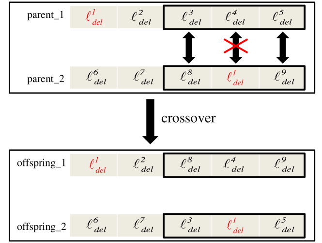
  Figure 6: Crossover of chromosomes in the perspective of deleted links. Red genotype will encounter collision after a direct exchange.

Input: $m$, $n_{iteration}$, $n_{elite}$, $n_{crossover}$, $n_{mutation}$, $pc$, and $pm$.

Output: population

1 Initialize population;

2 while not convergence or not reach to $n_{iteration}$ do

3      calculate the fitness of population;

4       retain $n_{elite}$ $elites$;

5       $Cro$ = Selection Operation($n_{crossover}$);

6       $\hat{Cro}$ = Crossover Operation($pc$, $Cro$);

7       $Mut$ = Selection Operation($n_{mutation}$);

8       $\hat{Mut}$ = Mutation Operation($pm$, $Mut$);

9       population = $elites\cup\hat{Cro}\cup\hat{Mut}$ ;

10 end while

11return population;

Algorithm 4 GA for Link Perturbation

3.3.2 Estimation of Distribution Algorithm (EDA)

EDA is a new kind of random optimization algorithm based on statistics theory. EDA has obvious differences with GA. As mentioned above, GA applies the crossover operation to generate new individuals; however, EDA searches better individuals through preference sampling and statistical learning. Specifically, one samples $n_{estimation}$ individual chromosomes according to their fitness values and then estimates the probability distributions of the deleted links $P(\ell_{del})$ and inserted links $P(\ell_{add})$ based on simple statistics. Finally, one generates $n_{eda}$ chromosomes according to their respective distributions. The pseudo-codes of GA and EDA are described in Algorithms  4,  5 and  6.

Input: $m$, $n_{iteration}$, $n_{elite}$, $n_{estimation}$, $n_{eda}$, $n_{mutation}$, and $pm$.

Output: pop

1 Initialize population;

2 while not convergence or not reach to $n_{iteration}$ do

3      calculate the fitness of population;

4       retain $n_{elite}$ $elites$;

5       $\hat{Eda}$ = Generate Population($n_{estimation}$, $n_{eda}$);

6       $Mut$ = Selection Operation($n_{mutation}$);

7       $\hat{Mut}$ = Mutation Operation($pm$, $Mut$);

8       population = $elites\cup\hat{Eda}\cup\hat{Mut}$ ;

9 end while

10

11return pop;

Algorithm 5 EDA for Link Perturbation

Input: $n_{estimation}$ and $n_{eda}$.

Output: population

1 Initialize population;

2 $Est$ = Selection Operation($n_{estimation}$);

3 Estimate the distributions of $P({\ell_{del}})$ and $P({\ell_{del}})$ by statistical sampling, where $P({\ell_{del}})\approx P({\ell_{del}}|Est)$ and $P({\ell_{del}})\approx P({\ell_{add}}|Est)$ ;

4 while not reach to $n_{eda}$ do

5      Sample $E_{del}$ and $E_{add}$ according to $P({\ell_{del}})$ and $P({\ell_{add}})$ respectively to generate new individual;

6 end while

7return population;

Algorithm 6 Generate Population

3.3.3 Accelerating the Fitness Calculation

Since one should calculate the fitness value for each individual at every iteration, the speed of fitness calculation directly affects the computational efficiency of the evolutionary algorithm. It is proposed here to accelerate the calculation of fitness by only recalculating the increment of the original network for each individual. Note that, for RA, deleting $(i,j)$ or inserting $(i,j)$ only affects the values of one-hop neighborhood.

Theorem 1.

Denote by $\tilde{N}^{recalc}_{ij}$ the set of node pairs whose RA values need to be recalculated in $\tilde{N}$. For the RA index, by either deleting or inserting $(i,j)$, one has $|\tilde{N}^{recalc}_{ij}|\leq\frac{1}{2}(k_{i}^{2}+k_{j}^{2}+k_{i}+k_{j})+1$.

Proof.

Assume that $(u,v)\in\tilde{N}^{recalc}_{ij}$, and denote by $G$ the original network and by $\Gamma(i)$ the one-hop neighbors of node $i$ in $G$.

First, consider $(i,j)\in G$, and delete $(i,j)$ from $G$.

• $u=i$, $v=j$

  Before deleting $(i,j)$, one has $(i,j)\notin N$; after deleting $(i,j)$, one has $(i,j)\in\tilde{N}$. Thus, $RA_{uv}$ needs to be calculated.

• $u\neq i$, $v\neq j$

  If $i$ or $j\in\Gamma(u)\cap\Gamma(v)$ in $G$, then $RA_{uv}$ needs to be recalculated after deleting $(i,j)$ and $(u,v)\in\{(\Gamma(i),\Gamma(i)),(\Gamma(j),\Gamma(j))\}$; if $\{i,j\}\notin\Gamma(u)\cap\Gamma(v)$ in $G$, then $RA_{uv}$ needs not to be recalculated after deleting $(i,j)$.

• $u\neq i$, $v=j$

  If $i\in\Gamma(u)\cap\Gamma(j)$ in $G$, then $RA_{uv}$ needs to be recalculated after deleting $(i,j)$ and $(u,v)\in\{(\Gamma(i),j)\}$; if $i\notin\Gamma(u)\cap\Gamma(j)$ in $G$, then $RA_{uv}$ needs not to be recalculated after deleting $(i,j)$.

• $u=i$, $v\neq j$

  $(u,v)\in\{(i,\Gamma(j))$} by symmetry.

To sum up, $(u,v)\in\{(i,j),(\Gamma(i),\Gamma(i)),(\Gamma(j),\Gamma(j)),(\Gamma(i),j),\\ (i,\Gamma(j))\}$ and the same for inserting $(i,j)$. Therefore,

$$\left|{\tilde{N}_{ij}^{recalc}}\right| \leq \frac{1}{2}{k_{i}}({k_{i}}-1)+\frac{1}{2}{k_{j}}({k_{j}}-1)+({k_{i}}+{k_{j}})+1$$ (9)

$$= \frac{1}{2}(k_{i}^{2}+k_{j}^{2}+k_{i}+k_{j})+1\,.$$

∎

An example to illustrate the influence of deleting $(i,j)$ is shown in Fig. 7. The set $\tilde{N}$ of non-existent node pairs in the perturbed network can be written as

$${\tilde{N}} = N+E_{del}-E_{add}$$ (10)

$$= (N-{N^{recalc}_{ij}})+{N^{recalc}_{ij}}+({E_{del}}-{E_{add}})\,.$$

Thus, one only needs to recalculate the RA values in $N^{recalc}_{ij}$, $E_{del}$ and $E_{add}$, to update the fitness. Consequently, the complexity of calculating the similarity values of node pairs in the perturbed network is significantly reduced, approximately from $O({|V{|^{2}}})$ to $O({m{\langle k\rangle}^{2}})$, where $m$ is the number of deleted/inserted links and ${\langle k\rangle}$ is the average degree of $G$.

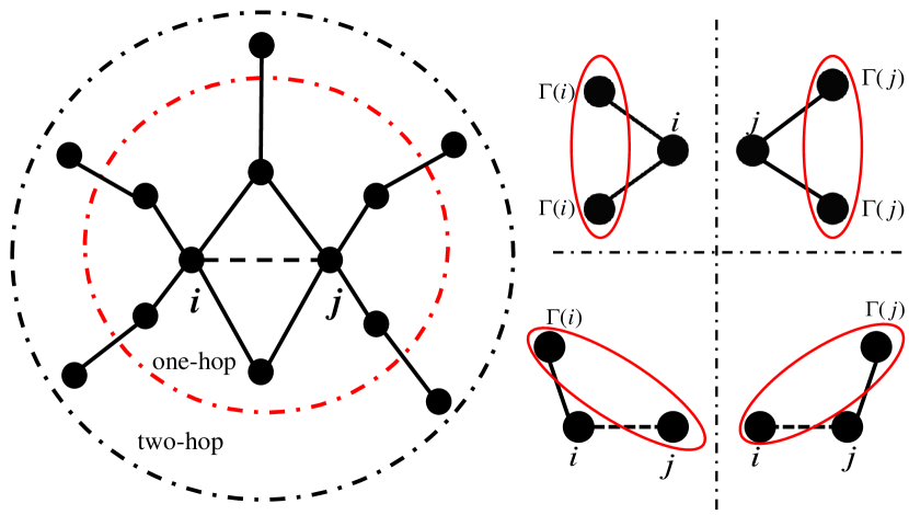
Figure 7: Left: neighborhood of $(i,j)$, where one-hop neighbors are within the red dashed circle. Right: four kinds of node pairs whose RA values need to be recalculated if $(i,j)$ is deleted or inserted.

4 Experiments and simulation results

TABLE I: Basic topological features of six networks. $|V|$ and $|E|$ are the numbers of nodes and edges, respectively; $\langle k\rangle$ is the average degree; $C$ is the clustering coefficient and $\langle d\rangle$ is the average distance.

	Mexican	Dolphin	Bomb	Lesmis	Throne	Jazz
$|V|$	35	62	64	77	107	198
$|E|$	117	159	243	254	352	2742
$\langle k\rangle$	6.686	5.129	7.594	6.597	6.597	27.697
$C$	0.448	0.259	0.622	0.573	0.551	0.617
$\langle d\rangle$	2.106	3.357	2.691	2.641	2.904	2.235

4.1 Data Description

Here, six networks are selected, with topological features shown in TABLE I.

• Mexican political elite (Mexican) is an undirected network, which contains the core of the political elite including the presidents and their closest collaborators. Links represent significant political, kinship, friendship, or business ties among them [32].

• Dolphin social network (Dolphin) is an undirected social network of dolphins living in a community and links present the frequent associations between pair-wise dolphins [33].

• Train Bombing (Bomb) is an undirected network, which contains contacts between suspected terrorists involved in the train bombing of Madrid on March 11, 2004, as reconstructed from newspapers. Nodes represent terrorists and link between two terrorists means that there was a contact between them [34].

• Lesmis is an undirected network of characters in Victor Hugo’s famous novel Les Miserables. Nodes denote characters and two nodes are connected if the corresponding characters co-appear in the same chapter of the book [35].

• Game of Thrones (Throne) is an undirected network of character interactions from the novel A Storm of Swords, where nodes denote the characters in the novel and a link denotes that two characters are mentioned together in the text [36].

• Jazz is a collaboration network of jazz musicians. Each node is a jazz musician and a link denotes that two musicians have played together in a band [37].

4.2 Simulation Results

4.2.1 Defense Effects of Various Link Perturbations

All links are randomly divided into 10 uniform and disjoint sets. One of the sets is selected as a validation set $E^{V}$ to be the set of sensitive links that need to be protected, and the rest is used as a training set $E^{T}$. Use the above-mentioned five methods including random, heuristic and evolutionary perturbations, respectively, to make a crosswise comparison.

TABLE II: Parameters settings for evolutionary algorithms, including GA and EDA, in each network.

$Item$	Meaning	Value
$\alpha$	weight in fitness	-
$m$	number of deleted/inserted links	-
$n_{iteration}$	number of iterations	1000
$e_{elite}$	number of retained elites	10
$n_{crossover}$	number of chromosomes for crossover	50
$n_{mutation}$	number of chromosomes for mutation	50
$pc$	crossover rate	0.7
$pm$	mutation rate	0.1
$n_{estimation}$	number of chromosomes for estimation	250
$n_{eda}$	number of generated population in EDA	50

In order that all links are used for both training and validation set, a 10-fold cross-validation is used to calculate the average precision and AUC. To ensure the sparsity of the perturbations, the proportion of deleted and inserted links in the training set are limited to observe the downtrend of defense effect with an increasing proportion of perturbations. The proportion is defined as the ratio of deleted/inserted links to all links in the training set. For example, if the proportion equals 0.1, it means that the deleted and inserted links account for 10% of the training set, respectively. To perform a reasonable comparison, add the perturbations using different methods in the same training set and then calculate the precision and AUC in the same validation set.

In Random Link Rewiring (RLR), randomly delete and insert a certain proportion of links in each training set and then repeat the procedure for one hundred times. In Randomly Link Swapping (RLS), conducting link swapping for one time means deleting two links and adding two other links at the same time. So, one may conduct half times of link swapping comparing to RLR and then repeat one hundred times of the procedure in each training set.

Figure 8: Average precision of each network perturbed by different methods with increasing proportions of deleted and inserted links.

Figure 9: Average AUC of each network perturbed by different methods with increasing proportions of deleted and inserted links.

In Heuristic Perturbation (HP), similarly conduct one hundred times of the procedure and then obtain the average precision and AUC. In GA and EDA, basic parameters of the evolutionary algorithms are set to be the empirical values, as shown in TABLE II. The main parameter to be tuned is the $\alpha$ in fitness, and the results are shown in TABLE III. It can be seen that there does not exist any fixed $\alpha$ that is optimal for all networks. So, one may select the value of $\alpha$ separately for each individual network. In the experiments, for Mexican, Dolphin, Lesmis and Throne, set $\alpha=0.01$; for Bomb, set $\alpha=1$; for Jazz, set $\alpha=0$. Then, repeat five times in each training set and calculate the average precision and AUC of the optimal individuals in the final population.

TABLE III: Average precision and AUC in each network with different values of $\alpha$ when the proportion of deleted and inserted equals 0.06.

Datasets(GA)		Precision				AUC
10
	$\alpha=0$	$\alpha=0.01$	$\alpha=0.1$	$\alpha=1$	$\alpha=0$	$\alpha=0.01$	$\alpha=0.1$	$\alpha=1$
Mexican		0.0818	0.0364	0.0364	0.0364	0.708	0.740	0.758	0.754
Dolphin	0.0667	0.00667	0.00667	0	0.698	0.741	0.749	0.752
Bomb	0.379	0.329	0.288	0.288	0.878	0.899	0.908	0.910
Lesmis	0.272	0.252	0.244	0.248	0.872	0.879	0.899	0.898
Throne	0.0943	0.0971	0.111	0.114	0.835	0.863	0.869	0.876
Jazz	0.397	0.422	0.439	0.417	0.952	0.956	0.958	0.958
Datasets(EDA)		Precision				AUC
10
	$\alpha=0$	$\alpha=0.01$	$\alpha=0.1$	$\alpha=1$	$\alpha=0$	$\alpha=0.01$	$\alpha=0.1$	$\alpha=1$
Mexican		0.0727	0.0273	0.0273	0.0364	0.701	0.745	0.744	0.744
Dolphin	0.0533	0.00667	0.00667	0	0.689	0.736	0.748	0.752
Bomb	0.392	0.317	0.225	0.129	0.867	0.897	0.909	0.905
Lesmis	0.276	0.224	0.156	0.0680	0.859	0.894	0.889	0.889
Throne	0.0886	0.0771	0.0314	0.0343	0.816	0.884	0.879	0.869
Jazz	0.401	0.434	0.429	0.425	0.951	0.959	0.957	0.955

The final results are shown in Fig. 8 and Fig. 9, from which it is found that evolutionary perturbations, especially those obtained by EDA, are superior to RLR, RLS and HP on most network datasets. The simulation results also show that the effect of HP is getting better as the proportion of perturbations increases. Especially, in a larger scale network with a larger validation set $E^{V}$, HP even outperforms evolutionary methods when measured in precision. Larger-scale perturbations in larger-scale networks mean that the search space is larger. Correspondingly, increasing the scale of the evolutionary method, e.g. increasing the numbers of individuals and iterations, may yield better results. However, time consumption can also exceed the allowable tolerance. Clearly, improving evolutionary methods or introducing parallel computing may reduce time consumption, which will be left for future studies.

Moreover, the running time before and after accelerating the fitness calculation has also been compared. In Fig. 10, experiments on GA and EDA with the same parameters in the two different networks indicate that the computational efficiency is increased significantly after acceleration.

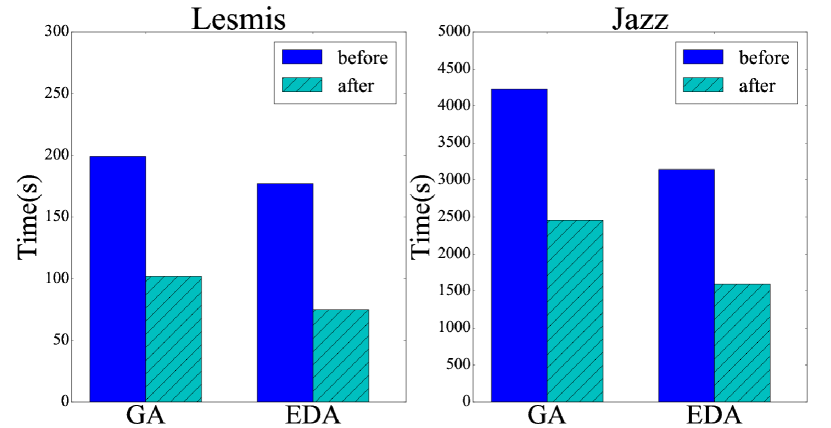
Figure 10: Average running time of GA and EDA with the same parameters in two networks before and after accelerating the fitness calculation.

4.2.2 Transferability of Evolutionary Perturbation

Although the above algorithms defend against specific link-prediction-based attacks (RA), an adversary may use other methods to do link prediction. Hence, it is desirable to know the transferability of the evolutionary perturbation especially acquired from EDA by checking the performance of other link prediction algorithms. For this purpose, the final perturbed networks obtained with the maximum perturbation generated by EDA together with HP are retained for each network, for which five different similarity indices are selected as test indices, which are Common Neighbors (CN), Jaccard, Preferential Attachment (PA), Adamic-Adar (AA) and Local Path (LP) [29], to calculate the average precision and AUC of the perturbed networks.

The results are summarized in TABLE IV. One can see that the transferability of EDA is better, no matter whether it is measured by precision or by AUC, comparing to the random perturbation (RLR/RLS) and heuristic perturbation (HP), in most networks. However, it can also be found that, in some cases, the transfer effect of EDA is inferior even than RLS when checked by LP, which may be due to the fact that LP considers the higher-order similarity of node pairs while the fitness of EDA only considers one-hop neighbors, which limits its transfer effect.

TABLE IV: Transferability of perturbations generated by HP and EDA measured by different similarity indices for each network. HP (RA) means HP is based on RA and EDA (RA) means that the fitness of EDA is based on RA as well.

Mexican			Precision					AUC
12
	original	RLR	RLS	HP(RA)	EDA(RA)	original	RLR	RLS	HP(RA)	EDA(RA)
RA			0.155	0.125	0.128	0.0182	0	0.777	0.734	0.732	0.721	0.495
CN	0.118	0.0993	0.106	0.0273	0	0.760	0.720	0.715	0.702	0.516
Jaccard	0.109	0.0876	0.0796	0.0273	0	0.752	0.709	0.701	0.693	0.496
PA	0.0546	0.0677	0.0596	0.0364	0.0300	0.625	0.616	0.625	0.588	0.557
AA	0.127	0.120	0.119	0.0182	0	0.776	0.733	0.731	0.721	0.504
LP($\alpha=0.5$)	0.127	0.0896	0.105	0.0545	0.0165	0.729	0.692	0.682	0.684	0.564
Dolphin			Precision					AUC
12
	original	RLR	RLS	HP(RA)	EDA(RA)	original	RLR	RLS	HP(RA)	EDA(RA)
RA			0.107	0.0865	0.0885	0.00667	0	0.765	0.740	0.740	0.701	0.629
CN	0.113	0.0953	0.0954	0.0333	0	0.760	0.736	0.736	0.700	0.648
Jaccard	0.113	0.0920	0.0973	0.0200	0.00455	0.760	0.737	0.736	0.699	0.651
PA	0.0133	0.0121	0.0132	0	0	0.623	0.616	0.623	0.589	0.583
AA	0.133	0.0978	0.0999	0.0133	0	0.765	0.741	0.741	0.702	0.632
LP($\alpha=0.5$)	0.120	0.107	0.103	0.0533	0.0226	0.792	0.768	0.762	0.772	0.711
Bomb			Precision					AUC
12
	original	RLR	RLS	HP(RA)	EDA(RA)	original	RLR	RLS	HP(RA)	EDA(RA)
RA			0.713	0.395	0.438	0.104	0.00182	0.929	0.909	0.904	0.903	0.891
CN	0.571	0.452	0.483	0.271	0.317	0.915	0.897	0.888	0.891	0.883
Jaccard	0.475	0.359	0.327	0.292	0.274	0.912	0.894	0.886	0.876	0.874
PA	0.229	0.186	0.219	0.138	0.139	0.774	0.767	0.774	0.749	0.744
AA	0.658	0.459	0.498	0.200	0.197	0.926	0.907	0.901	0.902	0.891
LP($\alpha=0.5$)	0.488	0.379	0.389	0.404	0.325	0.880	0.864	0.848	0.868	0.851
Lesmis			Precision					AUC
12
	original	RLR	RLS	HP(RA)	EDA(RA)	original	RLR	RLS	HP(RA)	EDA(RA)
RA			0.540	0.365	0.378	0.180	0.0199	0.914	0.898	0.896	0.891	0.879
CN	0.484	0.359	0.357	0.204	0.182	0.906	0.895	0.888	0.881	0.881
Jaccard	0.0360	0.202	0.0606	0.0920	0.114	0.914	0.870	0.859	0.854	0.850
PA	0.104	0.0936	0.102	0.0800	0.0768	0.782	0.780	0.782	0.768	0.777
AA	0.524	0.380	0.378	0.192	0.111	0.912	0.898	0.893	0.888	0.886
LP($\alpha=0.5$)	0.376	0.311	0.300	0.316	0.236	0.875	0.871	0.856	0.867	0.869
Throne			Precision					AUC
12
	original	RLR	RLS	HP(RA)	EDA(RA)	original	RLR	RLS	HP(RA)	EDA(RA)
RA			0.274	0.180	0.198	0.0343	0.0291	0.912	0.878	0.875	0.873	0.859
CN	0.200	0.174	0.181	0.109	0.103	0.892	0.865	0.859	0.849	0.847
Jaccard	0.0600	0.0553	0.0414	0.0543	0.0357	0.861	0.837	0.825	0.813	0.813
PA	0.123	0.110	0.122	0.100	0.0929	0.769	0.767	0.769	0.764	0.754
AA	0.240	0.192	0.203	0.0486	0.0814	0.908	0.878	0.873	0.869	0.859
LP($\alpha=0.5$)	0.163	0.145	0.157	0.117	0.116	0.867	0.852	0.838	0.860	0.845
Jazz			Precision					AUC
12
	original	RLR	RLS	HP(RA)	EDA(RA)	original	RLR	RLS	HP(RA)	EDA(RA)
RA			0.512	0.390	0.395	0.172	0.327	0.960	0.950	0.948	0.946	0.940
CN	0.497	0.382	0.378	0.237	0.335	0.954	0.938	0.930	0.933	0.929
Jaccard	0.512	0.390	0.398	0.275	0.342	0.960	0.945	0.942	0.926	0.938
PA	0.132	0.121	0.130	0.106	0.112	0.770	0.761	0.769	0.746	0.752
AA	0.518	0.391	0.391	0.220	0.336	0.961	0.944	0.938	0.939	0.935
LP($\alpha=0.5$)	0.359	0.295	0.281	0.265	0.264	0.908	0.889	0.874	0.902	0.882

5 Conclusions and research outlook

In this paper, a target defense algorithm against link-prediction-based attacks is proposed for social networks. Both heuristic and evolutionary perturbations techniques are used, taking into account both defense effect and data utility. A special fitness function is designed, which can simultaneously measure two link prediction indices, i.e. precision and AUC, and can reduce computation time by calculating variations after perturbations. The experimental results on six real-world networks show that evolutionary perturbations, especially those obtained by EDA, outperform other baseline methods, for both precision and AUC measures, in most cases. Finally, the transfer effect of evolutionary perturbations generated by EDA is verified, showing that evolutionary perturbations are transferable and can be used to defend other link-prediction-based attacks when the similarity measure is closely related to the fitness index.

However, for large-scale networks, especially when the number of links to be hidden is very large, the proposed algorithm does not take advantage of the network structure, consequently the evolutionary efficiency is limited. Therefore, improving evolutionary methods or introducing parallel computing so as to reduce computation time are good topics for future studies.

References

- [1] M. E. J. Newman, “The structure and function of complex networks,” SIAM Review, vol. 45, no. 2, pp. 167–256, 2003.
- [2] S. Boccaletti, V. Latora, Y. Moreno, M. Chavez, and D. U. Hwang, “Complex networks: Structure and dynamics,” Physics Reports, vol. 424, no. 4-5, pp. 175–308, 2006.
- [3] S. H. Strogatz, “Exploring complex networks,” Nature, vol. 410, no. 6825, pp. 268–276, 2001.
- [4] H. Jeong, S. P. Mason, A.-L. Barabási, and Z. N. Oltvai, “Lethality and centrality in protein networks,” Nature, vol. 411, no. 6833, pp. 41–42, 2001.
- [5] R. Guimer and M. Sales-Pardo, “Missing and spurious interactions and the reconstruction of complex networks,” Proceedings of the National Academy of Sciences of the United States of America, vol. 106, no. 52, p. 22073, 2009.
- [6] Chengdu and Fribourg, “Emergence of local structures in complex network:common neighborhood drives the network evolution,” Acta Physica Sinica, vol. 60, no. 3, pp. 825–828, 2011.
- [7] B. Gallagher, H. Tong, T. Eliassi-Rad, and C. Faloutsos, “Using ghost edges for classification in sparsely labeled networks,” in ACM SIGKDD International Conference on Knowledge Discovery and Data Mining, 2008, pp. 256–264.
- [8] C. V. Mering, L. J. Jensen, B. Snel, S. D. Hooper, M. Foglierini, N. Jouffre, M. A. Huynen, and P. Bork, “String: known and predicted protein-protein associations, integrated and transferred across organisms,” in Database Issue, 2005, pp. 433–437.
- [9] L. Lü, M. Medo, C. H. Yeung, Y.-C. Zhang, Z.-K. Zhang, and T. Zhou, “Recommender systems,” Physics Reports, vol. 519, no. 1, pp. 1–49, 2012.
- [10] P. Resnick and H. R. Varian, “Recommender systems,” Communications of the ACM, vol. 40, no. 3, pp. 56–58, 1997.
- [11] H. Chen, X. Li, and Z. Huang, “Link prediction approach to collaborative filtering,” in Proceedings of the 5th ACM/IEEE-CS Joint Conference on Digital Libraries. IEEE, 2005, pp. 141–142.
- [12] H. H. Song, T. W. Cho, V. Dave, Y. Zhang, and L. Qiu, “Scalable proximity estimation and link prediction in online social networks,” in Proceedings of the 9th ACM SIGCOMM Conference on Internet Measurement Conference. ACM, 2009, pp. 322–335.
- [13] W. Cukierski, B. Hamner, and B. Yang, “Graph-based features for supervised link prediction,” in Proceedings of the International Joint Conference on Neural Networks. IEEE, 2011, pp. 1237–1244.
- [14] X. Wu, X. Zhu, G. Q. Wu, and W. Ding, “Data mining with big data,” IEEE Transactions on Knowledge & Data Engineering, vol. 26, no. 1, pp. 97–107, 2014.
- [15] Q. Xuan, M. Zhou, Z.-Y. Zhang, C. Fu, Y. Xiang, Z. Wu, and V. Filkov, “Modern food foraging patterns: Geography and cuisine choices of restaurant patrons on yelp,” IEEE Transactions on Computational Social Systems, vol. 5, no. 2, pp. 508–517, 2018.
- [16] Q. Xuan, Z. Y. Zhang, C. Fu, H. X. Hu, and V. Filkov, “Social synchrony on complex networks.” IEEE Transactions on Cybernetics, vol. 48, no. 5, pp. 1420–1431, 2018.
- [17] K. Liu and E. Terzi, “Towards identity anonymization on graphs,” in ACM SIGMOD International Conference on Management of Data, 2008, pp. 93–106.
- [18] J. Cheng, W. C. Fu, and J. Liu, “K-isomorphism:privacy preserving network publication against structural attacks,” in ACM SIGMOD International Conference on Management of Data, SIGMOD 2010, Indianapolis, Indiana, USA, June, 2010, pp. 459–470.
- [19] C. H. Tai, P. S. Yu, D. N. Yang, and M. S. Chen, “Privacy-preserving social network publication against friendship attacks,” in ACM SIGKDD International Conference on Knowledge Discovery and Data Mining, 2011, pp. 1262–1270.
- [20] E. Zheleva and L. Getoor, “Preserving the privacy of sensitive relationships in graph data,” in Privacy, Security, and Trust in KDD. Springer, 2008, pp. 153–171.
- [21] M. Hay, G. Miklau, D. Jensen, P. Weis, and S. Srivastava, “Anonymizing social networks,” Computer Science Department Faculty Publication Series, p. 180, 2007.
- [22] X. Ying and X. Wu, “Randomizing social networks: a spectrum preserving approach,” in SIAM International Conference on Data Mining, SDM 2008, April 24-26, 2008, Atlanta, Georgia, Usa, 2008, pp. 739–750.
- [23] ——, “On link privacy in randomizing social networks,” in Pacific-Asia Conference on Knowledge Discovery and Data Mining. Springer, 2009, pp. 28–39.
- [24] A. M. Fard, K. Wang, and P. S. Yu, “Limiting link disclosure in social network analysis through subgraph-wise perturbation,” in Proceedings of the 15th International Conference on Extending Database Technology. ACM, 2012, pp. 109–119.
- [25] A. M. Fard and K. Wang, “Neighborhood randomization for link privacy in social network analysis,” World Wide Web, vol. 18, no. 1, pp. 9–32, 2015.
- [26] M. Fire, G. Katz, L. Rokach, and Y. Elovici, “Links reconstruction attack,” in Security and Privacy in Social Networks. Springer, 2013, pp. 181–196.
- [27] A. Rapoport, “Spread of information through a population with socio-structural bias: I. assumption of transitivity,” The Bulletin of Mathematical Biophysics, vol. 15, no. 4, pp. 523–533, 1953.
- [28] T. Zhou, L. Lü, and Y.-C. Zhang, “Predicting missing links via local information,” The European Physical Journal B-Condensed Matter and Complex Systems, vol. 71, no. 4, pp. 623–630, 2009.
- [29] L. Lü and T. Zhou, “Link prediction in complex networks: A survey,” Physica A: Statistical Mechanics and its Applications, vol. 390, no. 6, pp. 1150–1170, 2011.
- [30] C. Fu, M. Zhao, L. Fan, X. Chen, J. Chen, Z. Wu, Y. Xia, and Q. Xuan, “Link weight prediction using supervised learning methods and its application to yelp layered network,” IEEE Transactions on Knowledge & Data Engineering, vol. PP, no. 99, pp. 1–1, 2018.
- [31] Q. Xuan, Y. Li, and T. J. Wu, “Optimal symmetric networks in terms of minimizing average shortest path length and their sub-optimal growth model,” Physica A Statistical Mechanics & Its Applications, vol. 388, no. 7, pp. 1257–1267, 2009.
- [32] J. Gil-Mendieta and S. Schmidt, “The political network in mexico ☆,” Social Networks, vol. 18, no. 18, pp. 355–381, 1996.
- [33] D. Lusseau, K. Schneider, O. J. Boisseau, P. Haase, E. Slooten, and S. M. Dawson, “The bottlenose dolphin community of doubtful sound features a large proportion of long-lasting associations,” Behavioral Ecology & Sociobiology, vol. 54, no. 4, pp. 396–405, 2003.
- [34] B. Hayes, “Computing science: Connecting the dots,” American Scientist, vol. 94, no. 5, pp. 400–404, 2006.
- [35] D. E. Knuth, The Stanford GraphBase: a platform for combinatorial computing. Addison-Wesley Reading, 1993, vol. 37.
- [36] A. Beveridge and J. Shan, “Network of thrones,” Math Horizons, vol. 23, no. 4, pp. 18–22, 2016.
- [37] P. M. Gleiser and L. Danon, “Community structure in jazz,” Advances in complex systems, vol. 6, no. 04, pp. 565–573, 2003.