Low-frequency spectroscopy for quantum multi-level systems

Abstract

A periodically driven quantum system with avoided level crossing experiences both non-adiabatic transitions and wave-function phase changes. These result in coherent interference fringes in the system’s occupation probabilities. For qubits, with repelling energy levels, such interference, named after Landau-Zener-Stückelberg-Majorana, displays arc-shaped resonance lines. In the case of a multi-level system with an avoided level crossing of the two lower levels, we demonstrate that the shape of the resonances can change from convex arcs to concave heart-shaped and harp-shaped resonance lines. Indeed, the whole energy spectrum determines the shape of such resonance fringes and this also provides insight on the slow-frequency system spectroscopy. As a particular example, we consider this for valley-orbit silicon quantum dots, which are important for the emerging field of valleytronics.

I Introduction

Quantum systems can be reliably prepared, controlled, and probed. The “simplest nonsimple quantum problem” Berry (1995) is arguably a driven two-level system (a qubit), which can be used for quantum sensing Degen et al. (2017) and quantum information Buluta et al. (2011). Due to the interplay of the non-adiabatic transitions between the energy levels and the accumulation of the wave-function phase changes, the interference fringes provide a convenient and powerful tool for controlling and probing both the quantum system and its environment. This technique, known as Landau-Zener-Stückleberg-Majorana (LZSM) interferometry Shevchenko et al. (2010), is ubiquitously applied to two-level quantum systems. (For several experimental realizations in both superconducting and semiconducting systems, see, e.g., Refs. [Oliver et al., 2005; Sillanpää et al., 2006; Wilson et al., 2007; Izmalkov et al., 2008; Sun et al., 2009; Stehlik et al., 2012; Gonzalez-Zalba et al., 2016].) However, a generalization of this approach to multi-level systems remains a mostly open and topical subject, to which we devote the present work.

In order for LZSM physics to be directly relevant, a multi-level system has to have a reasonable quasicrossing of the lower energy levels, also known as avoided level crossing. Usually, multi-level systems have either all levels coupled or all well separated. The former case contains transitions between all energy levels and is known as amplitude spectroscopy Berns et al. (2008); Satanin et al. (2012). In the latter case, with a significant energy-level separation, a slow drive would not produce non-adiabatic transitions due to negligibly small tunneling probabilities, described by the Landau-Zener (LZ) formula. The cure to this could be to “dress” the system with another, resonant, signal. Then, these conveniently prepared dressed levels could be slowly driven and probed by means of LZSM physics. This approach was demonstrated for superconducting qubits.Sun et al. (2011); Gong et al. (2016) One message we would like to convey here is that a multi-level system should be doubly driven: by a resonant dressing signal and a slow driving one. In different contexts, doubly-driven quantum systems were studied in Refs. [Greenberg, 2007; Greenberg and Il’ichev, 2008; Mefed, 1999; Tuorila et al., 2010; Silveri et al., 2013; Saiko et al., 2014; Neilinger et al., 2016], while other examples of driven multi-level systems, where LZSM physics is relevant, are Refs. [Jin-Dan et al., 2011; Stehlik et al., 2012; Kenmoe et al., 2013; Ashhab, 2016; Stehlik et al., 2016; Sinitsyn and Chernyak, 2017; Chatterjee et al., 2018; Bogan et al., 2018; Koski et al., 2018; Gramajo et al., 2018; Parafilo and Kiselev, ].

So, our aim here is to consider how a multi-level system can be reduced to a two-level one, being well separated from the upper ones but bearing information about them. Here, instead of considering a general case, we would rather focus on an example Berry (1995): silicon double quantum dots (DQDs) exploiting both orbital and valley degrees of freedom, which make them multi-level systems Yang et al. (2013); Burkard and Petta (2016); Zhao and Hu (2018); Mi et al. (2018). Such systems present a unique opportunity of using the valley degree of freedom, which is studied in the emerging field of valleytronics.Rozhkov et al. (2017)

The rest of the paper is organized as follows. We will start in Sec. II from a four-state Hamiltonian for a silicon orbital-valley DQD, Ref. [Burkard and Petta, 2016]. (Another example of a four-state system is a device with two coupled qubits, studied in Appendix A.) We will discuss how to prepare the DQD states for low-frequency LZSM spectroscopy by dressing them with a resonant signal, with details presented in Appendix B. The dressing allows to reduce the four-level system to a two-level one. Then, in Sec. III we adopt the formulas from Ref. [Shevchenko et al., 2010] for this case. In Sec. IV we discuss the interference fringes obtained. We will also analyze the shape of the resonant lines. For a generic dressed four-level system, these are expected to be harp-shaped, which is demonstrated here for the parameters used in the experiments in Ref. [Mi et al., 2018]. A particular case, with a symmetric Hamiltonian, is analyzed in Appendix C. We conclude with a discussion that these studies allow the means for low-frequency spectroscopy for multi-level quantum systems.

II Bare and dressed energy levels

Let us consider the four-state Hamiltonian for a silicon orbital-valley DQD [Burkard and Petta, 2016]:

$$H(t)=\!\left(\begin{array}[]{cccc}\frac{\epsilon(t)}{2}+E_{\mathrm{L}}&0&t_{\mathrm{d}}&t_{\mathrm{v}}\\ 0&\frac{\epsilon(t)}{2}&-t_{\mathrm{v}}&t_{\mathrm{d}}\\ t_{\mathrm{d}}&-t_{\mathrm{v}}&-\frac{\epsilon(t)}{2}+E_{\mathrm{R}}&0\\ t_{\mathrm{v}}&t_{\mathrm{d}}&0&-\frac{\epsilon(t)}{2}\end{array}\right)=H_{0}+V_{\mathrm{d}}(t)$$ (1)

with

$$V_{\mathrm{d}}(t)=\frac{1}{2}A_{\mathrm{d}}\sin\omega_{\mathrm{d}}t\sigma_{z}^{(1)},$$ (2)

where $\sigma_{k}^{(1)}=\sigma_{k}\otimes\sigma_{0}$, and the $\sigma_{k}$’s stand for the Pauli matrices. The $E_{\mathrm{L,R}}$ are the left/right dot valley splittings, $t_{\mathrm{d}}$ and $t_{\mathrm{v}}$ are the inter-dot and inter-valley tunnel couplings, respectively. The energy bias is chosen as

$$\epsilon(t)=\varepsilon_{0}+A\sin\omega t+A_{\mathrm{d}}\sin\omega_{\mathrm{d}}t\equiv\varepsilon+A_{\mathrm{d}}\sin\omega_{\mathrm{d}}t\text{, \ \ \ }\omega\ll\omega_{\mathrm{d}},$$ (3)

which contains both the resonant dressing drive with frequency $\omega_{\mathrm{d}}$ and the slow spectroscopy drive $\varepsilon=\varepsilon_{0}+A\sin\omega t$ with frequency $\omega\ll\omega_{\mathrm{d}}$. Our approach consists of two steps. In the first step (“dressing”), we will ignore the slow signal and consider $\varepsilon$ to be a time-independent value. We will demonstrate how to reduce this system to a two-level one. (For other similar cases, when a multi-level structure is reduced to a two-level system see Refs. [Qi et al., 2017; Pietikäinen et al., 2018].) After incorporating this fast drive as the dressing, we will then add the slow time dependence, contained in the variable $\varepsilon$.

Consider first the energy levels of our four-level system. These are the eigenstates of the Hamiltonian $H_{0}$. In the absence of tunneling, $t_{\mathrm{d}}=t_{\mathrm{v}}=0$, these are given by the diagonal matrix elements in Eq. (1). These are the four straight intersecting lines in Fig. 1. Non-zero tunneling lifts the degeneracies. For calculations in this work we choose the parameters for a silicon orbital-valley DQD from Ref. [Mi et al., 2018]: $E_{\mathrm{L}}=37.5~{}\mu\mathrm{eV}$, $E_{\mathrm{R}}=38.3~{}\mu\mathrm{eV}$, $t_{\mathrm{d}}=25.4~{}\mu\mathrm{eV}$, $t_{\mathrm{v}}=11.8~{}\mu\mathrm{eV}$. (Another possible realization of a four-level structure, describing a two-qubit system, is given in Appendix A.) The spectrum with these parameters is shown in Fig. 1. The chosen parameters, which enter the Hamiltonian (1), result in the minimal energy difference $\Delta_{0}=(E_{1}-E_{0})_{\min}=7.845~{}$GHz$\cdot h$, and this takes place at very small offset, $\varepsilon=\varepsilon^{\ast}=-4\cdot 10^{-3}~{}$GHz. (Since we use both energy and frequency units, we note, for convenience, that $1~{}\mu\mathrm{eV}=0.2418~{}$GHz$\cdot h$.) Such large splitting $\Delta_{0}$ does not allow low-frequency spectroscopy because, according to the adiabatic theorem and the LZ formula, there would be no excitation for low-frequency driving. So, we will first “dress” the “bare” spectrum in Fig. 1.

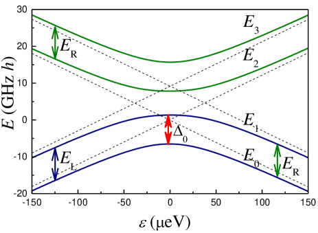
Figure 1: A four-level system: Energy levels of an orbital-valley DQD. The four energy levels in the absence of tunneling, $t_{\mathrm{d}}=t_{\mathrm{v}}=0$, shown by the dashed lines, experience four crossings. In general case, shown by the solid lines, the degeneracy is lifted, and the four energy levels $E_{i}$ are plotted for the parameters described in the text.

Accordingly, consider now the resonant driving with $\epsilon(t)=\varepsilon+A_{\mathrm{d}}\sin\omega_{\mathrm{d}}t$ and $\hbar\omega_{\mathrm{d}}\sim\Delta_{0}$. The detailed procedure is described in Appendix B. This results in the shift of the energy levels and the separation of the lower two levels from the upper ones. These become $\widetilde{E}_{0,1}=E_{0,1}\pm\hbar\omega_{\mathrm{d}}/2$. What matters for the low-frequency evolution then is the distance between these meaningful energy levels,

$$\Delta\widetilde{E}=\Delta E-\hbar\omega_{\mathrm{d}},$$ (4)

where $\Delta\widetilde{E}=\widetilde{E}_{1}-\widetilde{E}_{0}$ and $\Delta E=E_{1}-E_{0}$. Thus, we have mapped a multi-level system into a two-level dressed one.

To better compare with qubits, it is instructive to plot the equivalent (mirror-reflected) energy levels, $\pm\Delta\widetilde{E}/2$, with the same distance $\Delta\widetilde{E}$, instead of $\widetilde{E}_{0,1}$. The driving frequency should be taken close to $\Delta_{0}$, and then with $\omega_{\mathrm{d}}/2\pi=7.796~{}$GHz of [Mi et al., 2018], we have the dressed avoided level distance $\Delta=\Delta_{0}-\hbar\omega_{\mathrm{d}}=0.049~{}$GHz$\cdot h$. The dressed energy levels, featuring this avoided level crossing, are shown in Fig. 2(a) as a function of the energy bias $\varepsilon$.

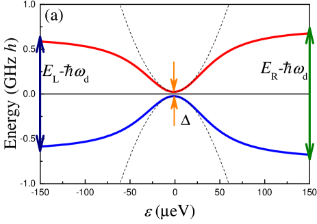
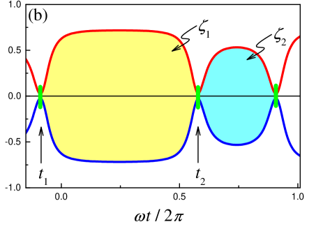
Figure 2: Dressed energy levels. In (a) the two lowest dressed states are shown by plotting $\pm\Delta\widetilde{E}/2$ versus $\varepsilon$, where $\Delta\widetilde{E}=\Delta E-\hbar\omega_{\mathrm{d}}$ and $\Delta E=E_{1}-E_{0}$. The distance between the dressed energy levels shows the avoided-level crossing $\Delta$ at around $\varepsilon=0$ and tends to $E_{\mathrm{L,R}}-\hbar\omega_{\mathrm{d}}$ to the left and right, respectively. The dashed parabolas correspond to the qubit-like spectrum at small $\varepsilon$. In (b) the same dressed energy levels are shown versus time for $\varepsilon=\varepsilon_{0}+A\sin\omega t$, with $\varepsilon_{0}=50~{}\mu\mathrm{eV}$ and $A=100~{}\mu\mathrm{eV}$. Several avoided-level crossings take place at $t=t_{1}$, $t_{2}$, and $t_{2}+2\pi/\omega$. The probabilistic LZ transitions are shown in these points by thick vertical green dashes. Between these avoided-level crossings, the wave-function phases $\zeta_{1,2}$ are accumulated. These phases, equal to the areas under the energy-level curves, result in observable interference fringes.

Close to the avoided level crossing, we can expand $\left(\Delta E\right)^{2}$ in series in $\varepsilon$ and obtain $\Delta\widetilde{E}=\sqrt{\Delta_{0}^{2}+0.16\varepsilon^{2}}-\hbar\omega_{\mathrm{d}}$. The respective curves are shown by the dashed lines in Fig. 2(a). This formula is useful for the description of the dynamics with $\varepsilon<E_{\mathrm{L,R}}$.

Hereafter, the slow signal, driving the qubit, will be taken with $\omega\sim\Delta$, so that to have a non-trivial LZ probability, $P_{\mathrm{LZ}}\sim 1$. Then $\varepsilon=\varepsilon_{0}+A\sin\omega t$ describes the low-frequency parametric time dependence of the energy levels. Imagine that we start at $\varepsilon=\varepsilon_{0}$ with, say, $\varepsilon_{0}=50~{}\mu\mathrm{eV}$ in Fig. 2(a). Then the dynamics corresponds to first increasing the bias $\varepsilon$ up to $\varepsilon=\varepsilon_{0}+A$, and then decreasing it to $\varepsilon=\varepsilon_{0}-A$. Respectively, the energy levels $\pm\frac{1}{2}\Delta\widetilde{E}(\varepsilon)$ will change, as shown in Fig. 2(b). Each time the system passes through $\varepsilon=0$ in Fig. 2(a), we have the avoided level crossing in Fig. 2(b). Such dynamics is described by the so-called adiabatic-impulse model, as detailed in Refs. [Ashhab et al., 2007; Shevchenko et al., 2010] and references therein. This model combines both intuitive clarity and quantitative accuracy. So, we devote the next section to this.

III LZSM for a multi-level system

We now would like to calculate the occupation probabilities for the two-level system with the energy levels $\pm\frac{1}{2}\Delta\widetilde{E}(\varepsilon)$, shown in Fig. 2. The adiabatic-impulse model considers the dynamics to be adiabatic, when far from the avoided level crossings, with non-adiabatic transitions at the points of minimal energy-level distance. The former stages are described by the accumulation of the wave-function phases, while the latter are characterized by the LZ transition formula. With this we can generalize the formulas for the slow-passage case from Refs. [Shevchenko et al., 2010, 2012], giving the upper-level time-averaged occupation probability

$$P_{+}=\frac{P_{\mathrm{LZ}}(1+\cos\zeta_{+}\cos\zeta_{-})}{\sin^{2}\zeta_{+}+2P_{\mathrm{LZ}}(1+\cos\zeta_{+}\cos\zeta_{-})},$$ (5)

where

$$\zeta_{+} = \zeta_{1}+\zeta_{2}+\varphi,\text{ }\zeta_{-}=\zeta_{1}-\zeta_{2},\text{ }$$ (6)

$$\zeta_{1} = \frac{1}{2\hbar}\int\limits_{t_{1}}^{t_{2}}\Delta\widetilde{E}(t)dt,\text{ }\zeta_{2}=\frac{1}{2\hbar}\int_{t_{2}}^{t_{1}+2\pi/\omega}\Delta\widetilde{E}(t)\;dt,$$

$$\Delta\widetilde{E} = E_{1}-E_{0}-\hbar\omega_{\mathrm{d}},\text{ }\varepsilon=\varepsilon_{0}+A\sin\omega t,$$

$$\omega t_{1} = \text{asin}\left(-\frac{\varepsilon_{0}}{A}\right),\text{ }\omega t_{2}=\pi-\omega t_{1},$$

$$\varphi = -\frac{\pi}{2}+2\delta(\ln\delta-1)+2\arg\Gamma(1-i\delta),$$

$$\delta = \frac{\Delta^{2}}{4v},\text{ }v=A\hbar\omega\sqrt{1-\left(\frac{\varepsilon_{0}}{A}\right)^{2}}.$$

And the probability of the non-adiabatic transition to the upper adiabatic level during the avoided level passage is given by the Landau-Zener formula $P_{\mathrm{LZ}}=\exp\left(-2\pi\delta\right)$. Here $\Gamma$ denotes the gamma function. Note that for sufficiently small frequency ($\delta\gg 1$) one could assume $\varphi\approx-\pi$, though in the equation above we keep the complete form of the phase, for the sake of generality.

Formula (5) defines the lines (arcs), along which the resonances are situated:

$$\zeta_{+}=k\pi.$$ (7)

Under this condition, the upper-level occupation probability becomes the highest possible, $P_{+}=1/2$. The width of the resonance lines is defined by the numerator in Eq. (5), which tends to zero when

$$\zeta_{1}=\frac{\pi}{2}+l\pi\text{ \ and \ \ }\zeta_{2}=\frac{\pi}{2}+m\pi,$$ (8)

where $l$ and $m$ are integers. Note that these intersect at $\zeta_{1}+\zeta_{2}=(l+m+1)\pi\equiv k\pi$, which means that the nodes are situated on the resonance lines, defined by Eq. (7). These are plotted in Fig. 3 for $\omega/2\pi=50$ MHz. The resonance line with $k=20$ is shown bolder in Fig. 3 to show that these are the harp-shaped resonance lines with convex shapes. Such harp-shaped resonances were reported recently in Ref. [Mi et al., 2018].

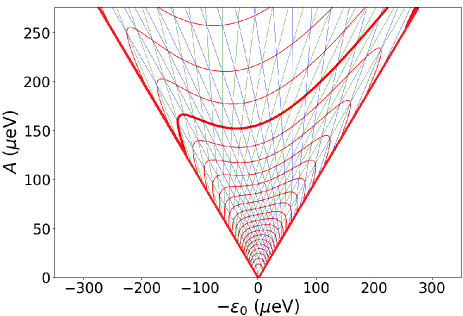
Figure 3: Harp-shaped resonance fringes and nodes. The position of the resonances is shown in red for different values of $k$, Eq. (7). These curves are equidistant arcs for small $k^{\prime}$s and harp-shaped lines with increasing distance for higher $k^{\prime}$s. When both phases $\zeta_{1,2}/\pi$ equal to half-integer numbers [Eq. (8)], the resonances are suppressed, and their positions are given by the intersection of the green and blue lines.

IV Discussion: relevance for low-frequency spectroscopy

The positions of the resonances in Fig. 3 bear information about the initial four-state Hamiltonian. Thus, these observations could be used for defining the system parameters, which effectively correspond to the spectroscopy of a multi-level system. Let us now summarize several distinctive features, which could be useful for this type of spectroscopy.

• The resonances are limited by the inclined lines, in the region $A>\left|\varepsilon_{0}-\varepsilon^{\ast}\right|$. This is because otherwise the avoided level crossing is not reached and there is no transition from the ground state to the excited one. The inclination of these lines could be useful for power calibration.

• For small driving amplitudes, $A<E_{\mathrm{L,R}}$, we have a qubit-like spectrum, and accordingly, the arcs are equidistant and symmetric.

• With increasing the driving amplitude, starting at $A\sim E_{\mathrm{L,R}}$, the resonances become asymmetric.

• With further increasing the driving amplitude, the shape of the resonance lines changes from convex to concave, producing harp-shaped curves. This is because the energy-level distance changes from increasing to becoming constant, see Fig. 2. In the symmetric case, with $E_{\mathrm{L}}=E_{\mathrm{R}}$, the curves are symmetric, and this case is analyzed in Appendix C.

• At large driving power, the resonance lines are increasingly separated. This can be conveniently studied along the line $\varepsilon_{0}=0$ in Fig. 3. This is done in Fig. 4. There, one can see the equidistant resonance position at smaller driving power $A$, as described by the inclined dashed line, and the increasing inter-resonance separation at larger $A$.

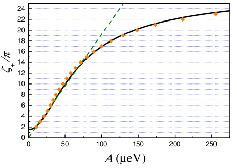
Figure 4: Power dependence of the resonances at zero offset, $\varepsilon_{0}=0$. The solid black curve is given by $\zeta_{+}$. The position of the resonances is defined by the equation $\zeta_{+}=k\pi$ and this corresponds to integer parts of $\zeta_{+}/\pi$, which are marked as horizontal grid lines. At low bias, i.e. for $k\leq 15$, these can be fit by the constant-slope green dashed line. This means that the resonance arcs are approximately equidistant. At higher driving power $A$, the inter-resonance distance monotonically increases. The orange diamonds correspond to the resonances from the experimental data in Fig. 2(a) of Ref. [Mi et al., 2018].

Our calculations are related to the experimental parameters of Ref. [Mi et al., 2018]. In particular, note the good agreement shown in Fig. 4. Moreover, our general approach can be applied to any other multi-level system. Our general formulation allows the flexible application to other systems, easy numerical calculations, as well as analytical analysis in various limiting cases. These are not possible by a direct numerical solution, without our more-analytical approach.

V Conclusion

We have demonstrated how a multi-level system could be reduced to a two-level one, by applying a resonant dressing signal. The obtained two-level system is remarkably distinct from a qubit because at larger bias the energy levels become equally separated, and not repelling. This distinction results in that the resonance fringes follow harp-shaped lines. Since the dressed two levels bear information about the initial multi-state system, the unusual and versatile properties of such interferometric features could be adopted for multi-level systems’ spectroscopy.

Appendix A A two-qubit four-level system

While multi-level quantum systems could be found in different contexts, we would like to present one additional example: a system of two coupled qubits. Let us now consider the Hamiltonian Denisenko et al. (2010); Temchenko et al. (2011); Gramajo et al. (2017)

$$H=-\frac{1}{2}\sum_{i=1,2}\left(\Delta_{i}\sigma_{x}^{(i)}+\varepsilon_{i}\sigma_{z}^{(i)}\right)+\frac{J}{2}\sigma_{z}^{(1)}\sigma_{z}^{(2)}=$$ (9)

$$=-\frac{1}{2}\!\left(\begin{array}[]{cccc}\!\varepsilon_{1}\!+\!\varepsilon_{2}\!-\!J\!&\Delta_{2}&\Delta_{1}&0\\ \Delta_{2}&\!\varepsilon_{1}\!-\!\varepsilon_{2}\!+\!J\!&0&\Delta_{1}\\ \Delta_{1}&0&\!-\!\varepsilon_{1}\!+\!\varepsilon_{2}\!+\!J\!&\Delta_{2}\\ 0&\Delta_{1}&\Delta_{2}&\!-\!\varepsilon_{1}\!-\!\varepsilon_{2}\!-\!J\!\end{array}\right),$$ (14)

where $\sigma_{k}^{(1)}=\sigma_{k}\otimes\sigma_{0}$ and $\sigma_{k}^{(2)}=\sigma_{0}\otimes\sigma_{k}$. Let us choose $\varepsilon_{2}$ to be a constant and $\varepsilon_{1}$ to have an alternating value: $\varepsilon_{2}=J$ (just for simplification) and

$$\varepsilon_{1}\equiv\varepsilon=\varepsilon_{0}+A\sin\omega t.$$ (15)

This would make the Hamiltonian somewhat resembling the one in Eq. (1). Then the Hamiltonian becomes

$$H=-\frac{1}{2}\!\left(\begin{array}[]{cccc}\varepsilon&\Delta_{2}&\Delta_{1}&0\\ \Delta_{2}&\varepsilon&0&\Delta_{1}\\ \Delta_{1}&0&-\varepsilon+2J&\Delta_{2}\\ 0&\Delta_{1}&\Delta_{2}&-\varepsilon-2J\end{array}\right)=H_{0}+V_{\mathrm{d}}(t)$$ (16)

with

$$V_{\mathrm{d}}(t)=-\frac{1}{2}A\sin\omega t\sigma_{z}^{(1)}.$$ (17)

In Fig. 5 we choose: $\Delta_{\mathrm{1}}/h=0.1$ GHz, $\Delta_{\mathrm{2}}/h=1$ GHz, and $J/h=0.2$ GHz. Such parameters give the minimal splitting $\Delta/h=73$ MHz and the shift $\varepsilon^{\ast}/h=93$ MHz. The lowest eigenvalues of $H_{0}$, denoted by $E_{0}$ and $E_{1}$, are shown as the red and blue curves in Fig. 5.

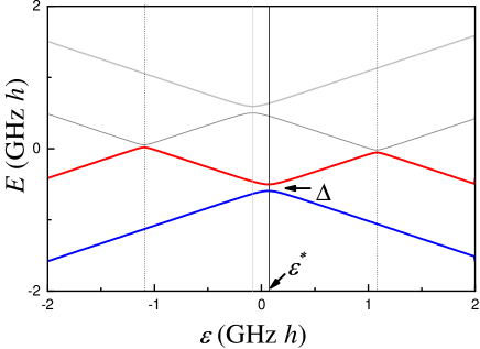
Figure 5: Energy levels of a two-qubit system. These are shown as an example of the situation where the lower two energy levels have a small avoided level crossing $\Delta$ and the distance between the energy levels increases at around this point and tends to constants at high values of the bias $\varepsilon$.

Note that for a two-qubit four-level system, the energy levels are similar to the ones presented in Fig. 2(a), in that they have small avoided level crossing, an increasing energy-level distance for small bias, and a constant distance for higher bias. An important distinction is that these bare levels are not separated from the upper ones. Transitions to the upper states would produce additional interference fringes like in Refs. [Berns et al., 2008; Satanin et al., 2012].

Appendix B Dressing

In this Appendix we consider how the resonantly driven four-state DQD can be reduced to a dressed two-level system. We start from the time-dependent Hamiltonian, Eq. (1) with $\epsilon(t)=\varepsilon+A_{\mathrm{d}}\sin\omega_{\mathrm{d}}t$, with $\varepsilon$ assumed here being time-independent, $H_{0}$ corresponds to $\epsilon(t)\rightarrow\varepsilon$, and

$$V_{\mathrm{d}}(t)=\frac{1}{2}A_{\mathrm{d}}\cos\left(\omega_{\mathrm{d}}t\right)\sigma_{z}^{(1)}$$ (18)

with $\sigma_{z}^{(1)}=\sigma_{z}\otimes\sigma_{0}$. The stationary Hamiltonian $H_{0}$ is diagonalized by the matrix $S$ (which can be found numerically):

$$S^{{\dagger}}H_{0}S=H_{0}^{\prime}=\mathrm{diag}(E_{0},E_{1},E_{2},E_{3}).$$ (19)

Then, the same procedure should be done with $V_{\mathrm{d}}(t)$; we denote the matrix $V=S^{{\dagger}}\sigma_{z}^{(1)}S$. And then, similarly to how this is done for qubits, e.g. in Ref. [Shevchenko et al., 2014], we make the unitary transformation $U=\exp\left(i\omega_{\mathrm{d}}t\sigma_{z}^{(2)}/2\right)$ and omit the fast-rotating terms, which means the rotating-wave approximation. We obtain the Hamiltonian of the dressed DQD:

$$\widetilde{H} = \left(\begin{array}[]{cccc}E_{0}+\frac{\hbar\omega_{\mathrm{d}}}{2}&&&0\\ &E_{1}-\frac{\hbar\omega_{\mathrm{d}}}{2}&&\\ &&E_{2}+\frac{\hbar\omega_{\mathrm{d}}}{2}&\\ 0&&&E_{3}-\frac{\hbar\omega_{\mathrm{d}}}{2}\end{array}\right)$$ (29)

$$+\frac{A_{\mathrm{d}}}{4}\left(\begin{array}[]{cccc}0&0&V_{02}&V_{03}\\ 0&0&V_{12}&V_{13}\\ V_{20}&V_{21}&0&0\\ V_{30}&V_{31}&0&0\end{array}\right).$$

Here $V_{ij}$ are the elements of the matrix $V$.

If we neglect the driving amplitude, $A_{\mathrm{d}}\rightarrow 0$, the dressed energy levels are given by the shifted bare ones: $\widetilde{E}_{i}=E_{i}\pm\hbar\omega_{\mathrm{d}}$. These are plotted in Fig. 6(a). The effect of the driving, for non-zero $A_{\mathrm{d}}$, is shown in Fig. 6(b) for the lowest two levels and $A_{\mathrm{d}}/\Delta=2$.

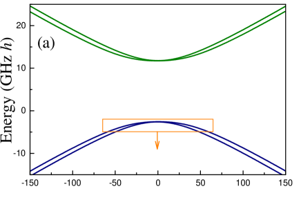
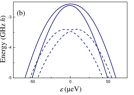
Figure 6: Energy levels of the dressed DQD. (a) At low driving power, $A_{\mathrm{d}}\rightarrow 0$, these are defined by $E_{i}\pm\hbar\omega_{\mathrm{d}}/2$, see Eq. (29). (b) Close-up of the lowest two dressed energy levels. The solid lines are the same as in (a), for low driving power. This displays the minimal energy-level distance at around $\varepsilon_{0}=0$ given by $\Delta=(E_{1}-E_{0})_{\min}-\hbar\omega_{\mathrm{d}}$. The dashed lines show how the driving changes the dressed energy levels; these are plotted for $A_{\mathrm{d}}/\Delta=2$.

Figure 6(a) demonstrates that the lowest two dressed states are well isolated from the upper ones. This allows to limit the description of our system to two levels only,

$$\widetilde{E}_{0,1}=E_{0,1}\pm\frac{\hbar\omega_{\mathrm{d}}}{2}.$$ (30)

The distance between these levels is

$$\Delta\widetilde{E}=\Delta E-\hbar\omega_{\mathrm{d}},$$ (31)

where $\Delta\widetilde{E}=\widetilde{E}_{1}-\widetilde{E}_{0}$ and $\Delta E=E_{1}-E_{0}$.

Appendix C Heart-shaped (concave) resonance fringes

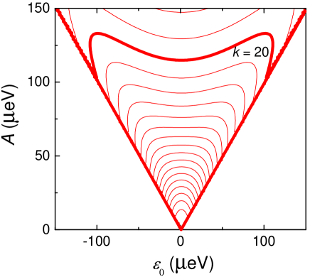
Figure 7: Resonances for a symmetric DQD. These are calculated analogously to the resonances shown in Fig. 3 with the only difference that $E_{\mathrm{L}}=E_{\mathrm{R}}=38.3~{}\mu$eV. Resonances with $k$ from $4$ to $22$ are shown. We make bolder the resonance line with $k=20$ to demonstrate that these are heart-shaped resonance lines with the convex shape at $\varepsilon_{0}=0$.

Consider a symmetric DQD, being the same orbital-valley one described by Eq. (1), with only one distinction that now we assume

$$E_{\mathrm{L}}=E_{\mathrm{R}}.$$ (32)

With this simplification, we can obtain expressions for the four energy levels

$$E_{0,1,2,3}=\frac{E_{\mathrm{R}}}{2}\pm\left\{\left[\frac{E_{\mathrm{R}}}{2}\pm\sqrt{\left(\frac{\varepsilon}{2}\right)^{2}+t_{\mathrm{d}}^{2}}\right]^{2}+t_{\mathrm{v}}^{2}\right\}^{1/2}.$$ (33)

By replacing the first sign $\pm$ for $-$, we have expressions for the lowest two levels, $E_{0,1}$. The difference between these energy levels at $\varepsilon=0$ is the minimal splitting:

$$\Delta_{0}=\sqrt{\left[\frac{E_{\mathrm{R}}}{2}+t_{\mathrm{d}}\right]^{2}+t_{\mathrm{v}}^{2}}-\sqrt{\left[\frac{E_{\mathrm{R}}}{2}-t_{\mathrm{d}}\right]^{2}+t_{\mathrm{v}}^{2}}.$$ (34)

Given this, for small $\varepsilon$ we can expand $\Delta E^{2}=\left(E_{1}-E_{0}\right)^{2}$ into series and obtain the spectrum

$$E_{1}-E_{0}\approx\sqrt{\Delta_{0}^{2}+0.16\varepsilon^{2}}.$$ (35)

Note that this is similar to a qubit spectrum $\sqrt{\Delta_{0}^{2}+\varepsilon^{2}}$, but differs by a numerical factor. In Fig. 2(a) we can see that the qubit-like spectrum, Eq. (35), is sufficient for describing the dressed energy levels at small values of the bias.

Symmetric heart-shaped resonances are shown in Fig. 7. Note that with increasing the driving amplitude, the resonance lines change from convex to concave shapes.

For the asymmetric case, with $E_{\mathrm{L}}\neq E_{\mathrm{R}}$, we can generalize Eq. (33) assuming

$$E_{0/1} = \theta(\varepsilon)\left\{\frac{E_{\mathrm{R}}}{2}-\left(\left[\frac{E_{\mathrm{R}}}{2}\pm\sqrt{\left(\frac{\varepsilon}{2}\right)^{2}+t_{\mathrm{d}}^{2}}\right]^{2}+t_{\mathrm{v}}^{2}\right)^{1/2}\right\}$$

$$+\theta(-\varepsilon)\left\{\frac{E_{\mathrm{L}}}{2}-\left(\left[\frac{E_{\mathrm{L}}}{2}\pm\sqrt{\left(\frac{\varepsilon}{2}\right)^{2}+t_{\mathrm{d}}^{2}}\right]^{2}+t_{\mathrm{v}}^{2}\right)^{1/2}\right\}.$$

For large values of the bias, $\varepsilon\rightarrow\infty$, equation (C) gives

$$E_{1}-E_{0}\approx\theta(\varepsilon)E_{\mathrm{R}}-\theta(-\varepsilon)E_{\mathrm{L}},$$ (37)

which correctly describes the spectrum, demonstrated in Fig. 2(a). Equation (C) can be useful for analytical studies.

References

- Berry (1995) M. Berry, “Two-state quantum asymptotics,” Annals of the New York Academy of Sciences 755, 303–317 (1995).
- Degen et al. (2017) C. L. Degen, F. Reinhard, and P. Cappellaro, “Quantum sensing,” Rev. Mod. Phys. 89, 035002 (2017).
- Buluta et al. (2011) I. Buluta, S. Ashhab, and F. Nori, “Natural and artificial atoms for quantum computation,” Rep. Prog. Phys. 74, 104401 (2011).
- Shevchenko et al. (2010) S. N. Shevchenko, S. Ashhab, and F. Nori, “Landau-Zener-Stückelberg interferometry,” Phys. Rep. 492, 1–30 (2010).
- Oliver et al. (2005) W. D. Oliver, Y. Yu, J. C. Lee, K. K. Berggren, L. S. Levitov, and T. P. Orlando, “Mach-Zehnder interferometry in a strongly driven superconducting qubit,” Science 310, 1653–1657 (2005).
- Sillanpää et al. (2006) M. Sillanpää, T. Lehtinen, A. Paila, Y. Makhlin, and P. Hakonen, “Continuous-time monitoring of Landau-Zener interference in a Cooper-pair box,” Phys. Rev. Lett. 96, 187002 (2006).
- Wilson et al. (2007) C. M. Wilson, T. Duty, F. Persson, M. Sandberg, G. Johansson, and P. Delsing, “Coherence times of dressed states of a superconducting qubit under extreme driving,” Phys. Rev. Lett. 98, 257003 (2007).
- Izmalkov et al. (2008) A. Izmalkov, S. H. W. van der Ploeg, S. N. Shevchenko, M. Grajcar, E. Il’ichev, U. Hübner, A. N. Omelyanchouk, and H.-G. Meyer, “Consistency of ground state and spectroscopic measurements on flux qubits,” Phys. Rev. Lett. 101, 017003 (2008).
- Sun et al. (2009) G. Sun, X. Wen, Y. Wang, S. Cong, J. Chen, L. Kang, W. Xu, Y. Yu, S. Han, and P. Wu, “Population inversion induced by Landau-Zener transition in a strongly driven rf superconducting quantum interference device,” Appl. Phys. Lett. 94, 102502 (2009).
- Stehlik et al. (2012) J. Stehlik, Y. Dovzhenko, J. R. Petta, J. R. Johansson, F. Nori, H. Lu, and A. C. Gossard, “Landau-Zener-Stückelberg interferometry of a single electron charge qubit,” Phys. Rev. B 86, 121303 (2012).
- Gonzalez-Zalba et al. (2016) M. F. Gonzalez-Zalba, S. N. Shevchenko, S. Barraud, J. R. Johansson, A. J. Ferguson, F. Nori, and A. C. Betz, “Gate-sensing coherent charge oscillations in a silicon field-effect transistor,” Nano Lett. 16, 1614–1619 (2016).
- Berns et al. (2008) D. M. Berns, M. S. Rudner, S. O. Valenzuela, K. K. Berggren, W. D. Oliver, L. S. Levitov, and T. P. Orlando, “Amplitude spectroscopy of a solid-state artificial atom,” Nature 455, 51 (2008).
- Satanin et al. (2012) A. M. Satanin, M. V. Denisenko, S. Ashhab, and F. Nori, “Amplitude spectroscopy of two coupled qubits,” Phys. Rev. B 85, 184524 (2012).
- Sun et al. (2011) G. Sun, X. Wen, B. Mao, Y. Yu, J. Chen, W. Xu, L. Kang, P. Wu, and S. Han, “Landau-Zener-Stückelberg interference of microwave-dressed states of a superconducting phase qubit,” Phys. Rev. B 83, 180507 (2011).
- Gong et al. (2016) M. Gong, Y. Zhou, D. Lan, Y. Fan, J. Pan, H. Yu, J. Chen, G. Sun, Y. Yu, S. Han, and P. Wu, “Landau-Zener-Stückelberg-Majorana interference in a 3D transmon driven by a chirped microwave,” Appl. Phys. Lett. 108, 112602 (2016).
- Greenberg (2007) Y. S. Greenberg, “Low-frequency Rabi spectroscopy of dissipative two-level systems: Dressed-state approach,” Phys. Rev. B 76, 104520 (2007).
- Greenberg and Il’ichev (2008) Y. S. Greenberg and E. Il’ichev, “Quantum theory of the low-frequency linear susceptibility of interferometer-type superconducting qubits,” Phys. Rev. B 77, 094513 (2008).
- Mefed (1999) A. E. Mefed, “Spectrometer for studying NMR and relaxation in the doubly rotating frame,” Applied Magnetic Resonance 16, 411–426 (1999).
- Tuorila et al. (2010) J. Tuorila, M. Silveri, M. Sillanpää, E. Thuneberg, Y. Makhlin, and P. Hakonen, “Stark effect and generalized Bloch-Siegert shift in a strongly driven two-level system,” Phys. Rev. Lett. 105, 257003 (2010).
- Silveri et al. (2013) M. Silveri, J. Tuorila, M. Kemppainen, and E. Thuneberg, “Probe spectroscopy of quasienergy states,” Phys. Rev. B 87, 134505 (2013).
- Saiko et al. (2014) A. P. Saiko, R. Fedaruk, and S. A. Markevich, “Relaxation, decoherence, and steady-state population inversion in qubits doubly dressed by microwave and radiofrequency fields,” J. Phys. B 47, 155502 (2014).
- Neilinger et al. (2016) P. Neilinger, S. N. Shevchenko, J. Bogár, M. Rehák, G. Oelsner, D. S. Karpov, U. Hübner, O. Astafiev, M. Grajcar, and E. Il’ichev, “Landau-Zener-Stückelberg-Majorana lasing in circuit quantum electrodynamics,” Phys. Rev. B 94, 094519 (2016).
- Jin-Dan et al. (2011) C. Jin-Dan, W. Xue-Da, S. Guo-Zhu, and Y. Yang, “Landau-Zener-Stückelberg interference in a multi-anticrossing system,” Chinese Phys. B 20, 088501 (2011).
- Kenmoe et al. (2013) M. B. Kenmoe, H. N. Phien, M. N. Kiselev, and L. C. Fai, “Effects of colored noise on Landau-Zener transitions: Two- and three-level systems,” Phys. Rev. B 87, 224301 (2013).
- Ashhab (2016) S. Ashhab, “Landau-Zener transitions in an open multilevel quantum system,” Phys. Rev. A 94, 042109 (2016).
- Stehlik et al. (2016) J. Stehlik, M. Z. Maialle, M. H. Degani, and J. R. Petta, “Role of multilevel Landau-Zener interference in extreme harmonic generation,” Phys. Rev. B 94, 075307 (2016).
- Sinitsyn and Chernyak (2017) N. A. Sinitsyn and V. Y. Chernyak, “The quest for solvable multistate Landau-Zener models,” J.Phys. A: Math. Theor. 50, 255203 (2017).
- Chatterjee et al. (2018) A. Chatterjee, S. N. Shevchenko, S. Barraud, R. M. Otxoa, F. Nori, J. J. L. Morton, and M. F. Gonzalez-Zalba, “A silicon-based single-electron interferometer coupled to a fermionic sea,” Phys. Rev. B 97, 045405 (2018).
- Bogan et al. (2018) A. Bogan, S. Studenikin, M. Korkusinski, L. Gaudreau, P. Zawadzki, A. S. Sachrajda, L. Tracy, J. Reno, and T. Hargett, “Landau-Zener-Stückelberg-Majorana interferometry of a single hole,” Phys. Rev. Lett. 120, 207701 (2018).
- Koski et al. (2018) J. V. Koski, A. J. Landig, A. Palyi, P. Scarlino, C. Reichl, W. Wegscheider, G. Burkard, A. Wallraff, K. Ensslin, and T. Ihn, “Floquet spectroscopy of a strongly driven quantum dot charge qubit with a microwave resonator,” Phys. Rev. Lett. 121, 043603 (2018).
- Gramajo et al. (2018) A. L. Gramajo, D. Dominguez, and M. J. Sanchez, “Amplitude tuning of steady state entanglement in strongly driven coupled qubits,” Phys. Rev. A 98, 042337 (2018).
- (32) A. V. Parafilo and M. N. Kiselev, “Landau-Zener transitions and Rabi oscillations in a Cooper-pair box: Beyond two-level models,” arXiv:1807.11604 .
- Yang et al. (2013) C. H. Yang, A. Rossi, R. Ruskov, N. S. Lai, F. A. Mohiyaddin, S. Lee, C. Tahan, G. Klimeck, A. Morello, and A. S. Dzurak, “Spin-valley lifetimes in a silicon quantum dot with tunable valley splitting,” Nature Comm. 4, 2069 (2013).
- Burkard and Petta (2016) G. Burkard and J. R. Petta, “Dispersive readout of valley splittings in cavity-coupled silicon quantum dots,” Phys. Rev. B 94, 195305 (2016).
- Zhao and Hu (2018) X. Zhao and X. Hu, “Coherent electron transport in silicon quantum dots,” arXiv:1803.00749 (2018).
- Mi et al. (2018) X. Mi, S. Kohler, and J. R. Petta, “Electrically protected valley-orbit qubits in silicon,” arXiv:1805.04545 (2018).
- Rozhkov et al. (2017) A. V. Rozhkov, A. L. Rakhmanov, A. O. Sboychakov, K. I. Kugel, and F. Nori, “Spin-valley half-metal as a prospective material for spin valleytronics,” Phys. Rev. Lett. 119, 107601 (2017).
- Qi et al. (2017) Z. Qi, X. Wu, D. R. Ward, J. R. Prance, D. Kim, J. K. Gamble, R. T. Mohr, Z. Shi, D. E. Savage, M. G. Lagally, M. A. Eriksson, M. Friesen, S. N. Coppersmith, and M. G. Vavilov, “Effects of charge noise on a pulse-gated singlet-triplet qubit,” Phys. Rev. B 96, 115305 (2017).
- Pietikäinen et al. (2018) I. Pietikäinen, S. Danilin, K. S. Kumar, J. Tuorila, and G. S. Paraoanu, “Multilevel effects in a driven generalized Rabi model,” J. Low. Temp. Phys. 191, 354 (2018).
- Ashhab et al. (2007) S. Ashhab, J. R. Johansson, A. M. Zagoskin, and F. Nori, “Two-level systems driven by large-amplitude fields,” Phys. Rev. A 75, 063414 (2007).
- Shevchenko et al. (2012) S. N. Shevchenko, S. Ashhab, and F. Nori, “Inverse Landau-Zener-Stückelberg problem for qubit-resonator systems,” Phys. Rev. B 85, 094502 (2012).
- Denisenko et al. (2010) M. V. Denisenko, A. M. Satanin, S. Ashhab, and F. Nori, “Dynamics of interacting qubits in a strong alternating electromagnetic field,” Phys. Solid State 52, 2281–2286 (2010).
- Temchenko et al. (2011) E. A. Temchenko, S. N. Shevchenko, and A. N. Omelyanchouk, “Dissipative dynamics of a two-qubit system: Four-level lasing,” Phys. Rev. B 83, 144507 (2011).
- Gramajo et al. (2017) A. L. Gramajo, D. Dominguez, and M. J. Sanchez, “Entanglement generation through the interplay of harmonic driving and interaction in coupled superconducting qubits,” Eur. Phys. J. B 90, 255 (2017).
- Shevchenko et al. (2014) S. N. Shevchenko, G. Oelsner, Y. S. Greenberg, P. Macha, D. S. Karpov, M. Grajcar, U. Hübner, A. N. Omelyanchouk, and E. Il’ichev, “Amplification and attenuation of a probe signal by doubly dressed states,” Phys. Rev. B 89, 184504 (2014).