Two faces of greedy leaf removal procedure on graphs

Abstract

The greedy leaf removal (GLR) procedure on a graph is an iterative removal of any vertex with degree one (leaf) along with its nearest neighbor (root). Its result has two faces: a residual subgraph as a core, and a set of removed roots. While the emergence of cores on uncorrelated random graphs was solved analytically, a theory for roots is ignored except in the case of Erdös-Rényi random graphs. Here we analytically study roots on random graphs. We further show that, with a simple geometrical interpretation and a concise mean-field theory of the GLR procedure, we reproduce the zero-temperature replica symmetric estimation of relative sizes of both minimal vertex covers and maximum matchings on random graphs with or without cores.

I Introduction

As a quantitative approach to model the topology of interconnection and interaction among the constituents of complex systems in various nature, the paradigm of graphs and networks Bollobas-2002 ; Albert.Barabasi-RMP-2002 ; Newman-SIAM-2003 ; Boccaleti.Latora.Moreno.Chavez.Hwang-PhysRep-2006 ; Dorogovtsev.Goltsev-RMP-2008 ; Newman-2018 is a simple choice. Its two major topics are the percolation phenomena and the combinatorial optimization. A percolation problem on a graph Stauffer.Aharony-1994 , which tackles intrinsically geometrical transitions, focuses on the subgraph size after a local procedure of vertex and edge removal (equivalently a vertex and edge addition to an empty graph). Its analysis provides a structural perspective to the stability of interconnected systems upon internal fluctuation and external perturbation, further sheds light on the management of critical transitions in high-dimensional dynamical systems Scheffer-2009 . A well-known percolation problem is the emergence of the giant connected component (GCC) Molloy.Reed-RandStructAlgo-1995 ; Albert.Jeong.Barabasi-Nature-2000 ; Cohen.etal-PRL-2000 ; Callaway.etal-PRL-2000 . A combinatorial optimization problem on a graph Papadimitriou.Steiglitz-1998 ; Pardalos.Du.Graham-2013-2e usually concerns finding an optimal set of vertices or edges under a structural constraint. The difficulty in finding solutions leads to the study of computational complexity classes Garey.Johnson-1979 , whose typical examples are the polynomial and the non-deterministic polynomial-time-hard (NP-hard) problems. From an algorithmic sense, a polynomial problem has a proper solver with a computation time $t$ as a polynomial function of the underlying graph size $N$ ($t\sim N^{c}$ with a finite constant $c$), while finding a solution of a NP-hard problem in the worst case needs an exponential computation time in order of the underlying graph size $N$ ($t\sim e^{dN}$ with a finite constant $d$).

The focus of the paper is at the intersection between the percolation and the combinatorial optimization problems. Specifically, we consider the implication of the greedy leaf removal (GLR) procedure in the minimal vertex cover (MVC) and the maximum matching (MM) problems on undirected graphs. The MVC problem, which is a NP-hard problem, concerns finding vertex covers of a graph (sets of vertices to which all the edges of the graph are adjacent) of the minimal cardinality. A list of results is derived with exact methods Gazmuri-Network-1984 ; Harant-DiscreteMath-1998 ; Frieze-DiscreteMath-1990 , numerical approximations Takabe.Hukushima-JStatMech-2016 , and statistical physical methods (replica trick and cavity method) Mezard.Parisi.Virasoro-1987 ; Nishimori-2001 ; Mezard.Montanari-2009 ; Weigt.Hartmann-PRL-2000 ; Weigt.Hartmann-PRL-2001 ; Weigt.Hartmann-PRE-2001 ; Zhou-EPJB-2003 ; Zhou-PRL-2005 ; Weigt.Zhou-PRE-2006 ; Zhou.Zhou-PRE-2009 ; Zhang.Zeng.Zhou-PRE-2009 . Reviews with a statistical physical background can be found in Hartmann.Weigt-2005 ; Hartmann.Weigt-JPhyA-2003 ; Zhao.Zhou-CPB-2014 . The MM problem Lovasz.Plummer-1986 , which is a polynomial problem, concerns finding matchings on a graph (sets of edges sharing no common vertex) of the maximal size. Treatments of the problem with statistical physical methods Zhou.OuYang-arxiv-2003 ; Zdeborova.Mezard-JStatMech-2006 can be found therein. The GLR procedure on a graph Karp.Sipser-IEEFoCS-1981 ; Aronson.Frieze.Pittel-RandStrucAlgo-1998 iteratively removes any vertex with only one nearest neighbor (leaf) along with its sole nearest neighbor (root). It results in core percolation, whose mean-field theory on uncorrelated random graphs is developed in Bauer.Golinelli-EPJB-2001 ; Liu.Csoka.Zhou.Posfai-PRL-2012 . The GLR procedure is adopted as a local step to approximate MVCs and MMs Karp.Sipser-IEEFoCS-1981 ; Aronson.Frieze.Pittel-RandStrucAlgo-1998 ; Bauer.Golinelli-EPJB-2001 , and the core percolation corresponds to a fundamental transition in the organization of solution spaces of both optimization problems Weigt.Hartmann-PRL-2000 ; Weigt.Hartmann-PRL-2001 ; Weigt.Hartmann-PRE-2001 ; Zhou-EPJB-2003 ; Zhou-PRL-2005 ; Weigt.Zhou-PRE-2006 ; Zhou.Zhou-PRE-2009 ; Zhang.Zeng.Zhou-PRE-2009 ; Zhou.OuYang-arxiv-2003 ; Zdeborova.Mezard-JStatMech-2006 . The GLR procedure variants for combinatorial optimizations with concurrent percolation phenomena and solution space transitions also show in the MM problem of the network controllability Liu.Slotine.Barabasi-Nature-2011 ; Jia.etal-NatComm-2013 , the $p$-spin model and the XOR-SAT problem Mezard.RicciTersenghi.Zecchina-JStatPhys-2003 ; Cocco.etal-PRL-2003 , the Boolean networks Correale.etal-PRL-2006 ; Correale.etal-JStatMech-2006 , the maximum set packing problem Lucibello.RicciTersenghi-IntJStatMech-2014 , and the minimum dominating set problem Haynes.Hedetniemi.Slater-1998 ; Zhao.Zhou-JStatPhys-2015 ; Zhao.Zhou-LNCS-2015 ; Habibulla-JStatMech-2017 .

The GLR procedure leaves a core and a set of roots. A scenario with two faces also shows in the articulation points Tarjan.Vishkin-SIAMJComput-1985 ; Liu.etal-NatCommun-2017 and the $k$-core pruning process Chalupa.Leath.Reich-JPhysC-1979 ; Dorogovtsev.etal-PRL-2006 ; Baxter.etal-PRX-2015 . It is established that Karp.Sipser-IEEFoCS-1981 ; Bauer.Golinelli-EPJB-2001 : (1) on a graph without core, from roots we can reconstruct a MVC and a MM; correspondingly, the root size is just the MVC or MM size; (2) on a general graph, with its roots and core, we can estimate an average MM size based on the perfect matching of cores (each vertex in a core is adjacent to a matched edge). Yet unlike the core, the roots lack a general analytical treatment except on the Erdös-Rényi random graphs Karp.Sipser-IEEFoCS-1981 ; Bauer.Golinelli-EPJB-2001 , and the geometrical implication of roots and cores on estimating MVC and MM sizes is not fully explored. Here we sum our main contribution in this paper: (1) we complete the missing piece of an analytical theory of root sizes on uncorrelated random graphs; (2) based on the geometrical interpretation and the analytical theory of roots and cores, we develop simple frameworks to estimate MVC and MM fractions on random graphs, which retrieve their zero-temperature replica symmetric results from previous statistical physical literature.

The layout of the paper is as follows. In section II, we explain the GLR procedure, the MVC problem, and the MM problem. In section III, we lay down a mean-field theory for the two faces of the GLR procedure on uncorrelated random graphs, and its implication in estimating MVC and MM sizes. In section IV, we test our framework on some random graph models and real networks. In section V, we discuss and conclude the paper.

II Model

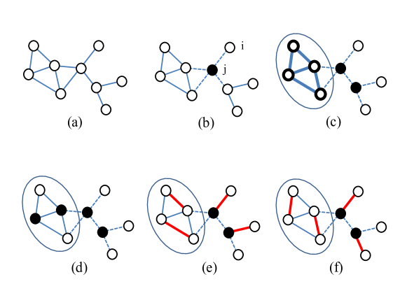
Figure 1: The GLR procedure, the MVCs, and the MMs on a small graph. (a) shows a graph with $9$ vertices and $11$ edges. (b) shows a single GLR step, in which the leaf $i$ and its neighboring root $j$ (in a filled circle) are removed along with their adjacent edges (in dashed lines). (c) shows the result of the GLR procedure, a set of $2$ roots (in filled circles) and a core consisting of $4$ vertices and $5$ edges (enclosed in a large circle). (d) shows a MVC as a set of $4$ vertices (in filled circles). (e) and (f) show two MMs both as a set of $4$ edges (in thick solid lines).

First we explain some notions for graphs. An undirected graph $G=\{V,E\}$ consists of a vertex set $V$ and an edge set $E\subset V\times V$. For an edge $(i,j)$ between the end-vertices $i$ and $j$, $i$ is a nearest neighbor of $j$, and vice versa. The degree $k_{i}$ of a vertex $i$ is the size of its nearest neighbors or $|\partial i|$. The degree distribution $P(k)$ is the probability of finding a randomly chosen vertex with a degree $k$. The mean degree or connectivity $c$ is the average degree of a vertex, or $c\equiv 2|E|/|V|=\sum_{k=0}^{\infty}kP(k)$. The excess degree distribution $Q(k)$ is the probability of arriving a vertex with a degree $k$ following a randomly chosen edge, equivalently $Q(k)=kP(k)/c$. We also define cavity graphs for a graph. The cavity graph $G\backslash i$ is the subgraph of $G$ with the vertex $i$ and all its adjacent edges removed, equivalently $\{V^{\prime},E^{\prime}\}$ with $V^{\prime}=V\backslash i$ and $E^{\prime}=E\backslash\{(k,i)\}$ with $k\in\partial i$. The cavity graph $G\backslash(i,j)$ is the subgraph of $G$ with the edge $(i,j)$ removed, equivalently $\{V,E^{{}^{\prime}}\}$ with $E^{{}^{\prime}}=E\backslash(i,j)$.

The GLR procedure consists of single iterative GLR steps in which a leaf and its neighboring root is removed along with all their adjacent edges, and finally leaves a subgraph as the core. Figures 1 (a) - (c) show an example. We should mention that Bauer.Golinelli-EPJB-2001 : the core of a graph is well defined, or the vertices and the edges in a core are independent of the GLR pruning process; the set of roots depends on the trajectory of the pruning process, yet on large graphs its size converges on average.

A vertex cover (VC) of $G$ is a set of vertices $\Gamma\subset V$ to which each edge in $E$ is adjacent. Taking the GLR procedure as a local method, in each step the root (such as the vertex $j$ in figure 1 (b)) is selected into a VC and all its adjacent edges are removed as satisfied constraints. If there is no core after the GLR procedure, the set of roots is simply a MVC; otherwise, local algorithms or statistical physical methods can be further applied on the core to approximate a MVC. Figure 1 (d) shows an example.

A matching of $G$ is a set of edges $\Delta\subset E$ without shared vertices. The GLR procedure serves as a component of the well-known Karp-Sipser algorithm Karp.Sipser-IEEFoCS-1981 , a randomized algorithm which finds MMs with a high probability on large graphs. The Karp-Sipser algorithm on a graph goes as: (1) the GLR procedure is applied on the current graph, while in each step the edge bridging a leaf and its neighboring root is selected into a matching; (2) an edge in the core is randomly selected into the matching, and any edge adjacent to its end-vertices is removed; (3) the above two steps are iteratively carried out until there is no edge left, and the resulted matching is an approximate MM. Figure 1 (e) and (f) show an example. If there is no core left on a graph, the MM size is simply the root size; otherwise, we can adopt the perfect matching of cores Karp.Sipser-IEEFoCS-1981 , which assumes that any vertex in a core is adjacent to a certain edge in the MM of the core. Taken together, the MM size on a large graph can be estimated conveniently as the root size plus half the core vertex size.

III Theory

As we can see, the GLR procedure applies on any undirected graph instance. Yet on uncorrelated random graphs, we can analytically calculate the size of roots by extending a cavity method for cores from the GLR procedure in Liu.Csoka.Zhou.Posfai-PRL-2012 . By further exploring the geometrical meaning of the roots and cores, we can develop analytical frameworks for both the MVC and MM sizes on random graphs.

III.1 GLR

On an uncorrelated random graph $G=\{V,E\}$ with a vertex set $V$ and an edge set $E$, we define two cavity probabilities tailored for the GLR procedure. Following a randomly chosen edge $(i,j)\in E$ from the vertex $i$ to the vertex $j$, we define $\alpha$ ($\beta$) as the probability that $j$ becomes a leaf (a root) in the GLR procedure on the cavity graph $G\backslash(i,j)$. On sparse random graphs, the local tree-structure approximation for the belief propagation algorithms Mezard.Montanari-2009 ; Bethe-ProcRSocLondA-1935 ; Kschischang.Frey.Loeliger-IEEETransInfTheor-2001 ; Yedidia.Freeman.Weiss-IEEETransInfTheor-2005 assumes that the states of the nearest neighbors of any vertex, say $i\in V$, are independent of each other in the pruning process on the cavity graph $G\backslash i$. Based on this approximation, we have the self-consistent equations of $\alpha$ and $\beta$ as

$$\alpha = \sum_{k=1}^{\infty}Q(k)\beta^{k-1},$$ (1)

$$\beta = 1-\sum_{k=1}^{\infty}Q(k)(1-\alpha)^{k-1}.$$ (2)

We define $n$ as the fraction of vertices in a core, $l$ the relative size of edges in a core normalized by the vertex size $|V|$, and $w$ the fraction of roots. In the framework of cavity method, these relative sizes can be calculated as marginal probabilities with the stable solutions of $\alpha$ and $\beta$. We have

$$n =\sum_{k=2}^{\infty}P(k)\sum_{s=2}^{k}\left(\begin{array}[]{c}k\\ s\end{array}\right)\beta^{k-s}(1-\alpha-\beta)^{s},$$ (5)

$$l =\frac{1}{2}c(1-\alpha-\beta)^{2},$$ (6)

$$w =1-\sum_{k=0}^{\infty}P(k)(1-\alpha)^{k}-\frac{1}{2}c\alpha^{2}.$$ (7)

Equation (5) can be reformulated as $n=\sum_{k=0}^{\infty}P(k)[(1-\alpha)^{k}-\beta^{k}]-c\alpha(1-\alpha-\beta)$.

Equations (1) and (2) have been derived in Zdeborova.Mezard-JStatMech-2006 and equations (1) - (6) in Liu.Csoka.Zhou.Posfai-PRL-2012 , yet equation (7) is our contribution here. Here is a simple explanation for them. For equations (1) and (2), we consider the case from a cavity graph $G\backslash j$ to another cavity graph $G\backslash(i,j)$ after some edge addition, in which $(i,j)\in E$ is a randomly chosen edge. If $j$ is a leaf on $G\backslash(i,j)$, all its nearest neighbors except $i$ must be removed as roots on $G\backslash j$, thus we have equation (1). In a similar sense, if the vertex $j$ is a root on $G\backslash(i,j)$, there must be at least one nearest neighbors except $i$ turning into leaves on $G\backslash j$, thus we have equation (2). We then consider the case from a cavity graph $G\backslash i$ to the original graph $G$ after some edge addition, in which $i\in V$ is a randomly chosen vertex. If a newly added vertex $i$ is in the core of $G$, among all the nearest neighbors of $i$, there must be no leaf, only roots, and at least two vertices in the core of $G\backslash i$ to forbid the GLR procedure, thus we have equation (5). If a newly added vertex $i$ is a root of $G$, among all the nearest neighbors of $i$ on $G\backslash i$, there must be at least one leaves, thus we have the first two terms on the right-hand side (RHS) of equation (7). Yet there is a recounting case. We consider the case from a cavity graph $G\backslash(i,j)$ to $G$, in which $(i,j)\in E$ is a randomly chosen edge. If $i$ and $j$ are both leaves on $G\backslash(i,j)$, they could be both counted as roots on $G$. The coefficient $c/2(=|E|/|V|)$ is the relative density of edges to vertices. Thus we have the third term on the RHS of equation (7). For equation (6), we also consider the case from $G\backslash(i,j)$ to $G$. If a newly added edge $(i,j)$ is in the core of $G$, both $i$ and $j$ must be in the core of $G\backslash(i,j)$. The coefficient $c/2$ follows the same logic in equation (7).

In appendix A, other than the cumulative approach in this section, we provide a discrete approach to the mean-field theory of the GLR procedure. This approach is based on the stepwise interpretation of the pruning process: at each time-step with an index $t\geq 0$, all the leaves are determined, their neighboring roots selected, and all their adjacent edges removed; the discrete steps are carried out iteratively until there is no leaf left at large $t$. The discrete viewpoint of a local process on graphs is adopted in various percolation and optimization problems Bauer.Golinelli-EPJB-2001 ; Zhao.Zhou-JStatPhys-2015 ; Zhao.Zhou-LNCS-2015 ; Liu.etal-NatCommun-2017 ; Baxter.etal-PRX-2015 . With the logic in equations (1) and (2), following a randomly chosen edge $(i,j)\in E$ from the vertex $i$ to the vertex $j$, we define $\alpha^{(t)}$ ($\beta^{(t)}$) with $t\geq 0$ as the cavity probabilities of $j$ to be a leaf (a root) at the $t$-th time-step of the discretized GLR procedure on the cavity graph $G\backslash(i,j)$. We can further calculate the relative sizes of the removed roots and the residual subgraph size at each time-step. In appendix A, we will show that in the case of infinitely large time-steps ($t\rightarrow\infty$), the discrete formulation reduces to the cumulative one in this section.

III.2 MVC

For the MVC problem on a graph, we denote $x$ as the relative size of a MVC (the size of vertices in a MVC normalized by the graph vertex size). It is an established result Karp.Sipser-IEEFoCS-1981 ; Bauer.Golinelli-EPJB-2001 that: if a graph has no core, the roots constitute a MVC; otherwise, the size of the roots provides a lower bound for MVCs. From an algorithmic perspective, on any graph instance we have

$$x=\left\{\begin{array}[]{rcl}w,&\mbox{for}&n=0;\\ w+x_{core},&\mbox{for}&n>0,\end{array}\right.$$ (10)

while $x_{core}$ is the MVC size of the core, which can be approximated efficiently with message-passing algorithms Weigt.Zhou-PRE-2006 ; Zhao.Zhou-CPB-2014 .

Besides the above obvious result, we can go deeper into the region of graphs with cores. An analysis of the fixed points of $\alpha$ and $\beta$ from equations (1) and (2) on infinitely large graphs shows that: before the core percolation, there is only one branch of fixed points as the stable solution, denoted as $(\alpha_{\textrm{M}},\beta_{\textrm{M}})$ with $1-\alpha_{\textrm{M}}-\beta_{\textrm{M}}=0$; after the core percolation, there are another two new branches of fixed points emerged as the lower branch $(\alpha_{\textrm{L}},\beta_{\textrm{L}})$ and the upper branch $(\alpha_{\textrm{U}},\beta_{\textrm{U}})$ with $\alpha_{\textrm{L}}<\alpha_{\textrm{M}}<\alpha_{\textrm{U}}$ and $1-\alpha_{\textrm{L}}-\beta_{\textrm{L}}=-(1-\alpha_{\textrm{U}}-\beta_{\textrm{U}})>0$, among which the lower branch of $(\alpha_{\textrm{L}},\beta_{\textrm{L}})$ acts as the stable one. Yet, the middle branch with $1-\alpha_{\textrm{M}}-\beta_{\textrm{M}}=0$ is always a solution of equations (1) and (2), under which $n=0$ and $w$ gives an estimation of $x$ on graphs with or without cores. We consider the solution branch with $1-\alpha-\beta=0$ (dropping the subscripts conveniently) as the trivial core condition, and the corresponding $w$ as the trivial core solution of the MVC problem. Taken together, from an analytical perspective, on large random graphs we have

$$x=w,\ \rm{s.t.}\ 1-\alpha-\beta=0.$$ (11)

Equations (1), (2), (7), and (11) constitute our framework to estimate the MVC sizes on random graphs with or without cores. On random graphs without cores, our framework gives the exact MVC sizes; otherwise, our framework is an underestimation of the MVC sizes. Later we will see that our framework simply reproduces the well-known zero-temperature replica symmetric estimation of the MVC sizes on Erdös-Rényi random graphs in Weigt.Hartmann-PRL-2000 .

We further estimate sizes of backbones in MVC solutions. With the notation in Weigt.Hartmann-PRL-2000 , we define the fraction of covered backbone $b_{+}$ as the relative size of vertices which are always in the MVC solutions, the fraction of uncovered backbone $b_{-}$ the relative size of vertices which are absent from any MVC solution. From a geometrical viewpoint, the covered backbone is simply the set of the roots excluding those from the isolated edges whose both end-vertices can be in a MVC solution, equivalently $b_{+}=w-c\alpha^{2}/2$, and the uncovered backbone is simply the set of the leaves. We have

$$b_{+} =1-\sum_{k=0}^{\infty}P(k)(1-\alpha)^{k}-c\alpha^{2},$$

$$b_{-} =\alpha,$$ (12)

$$\ \textrm{s.t.}\ 1-\alpha-\beta=0.$$

To compare our framework of MVC sizes with simulation on graph instances, we adopt a hybrid algorithm combining the GLR procedure and the belief propagation-guided decimation (BPD) algorithm Weigt.Zhou-PRE-2006 ; Zhao.Zhou-CPB-2014 . Details of the BPD algorithm is left in appendix B. The hybrid algorithm goes as: (1) on a given graph, the GLR procedure is applied and leaves a core; (2) the BPD algorithm is further applied on the core, during which a small number of vertices with the highest marginal probabilities to be in MVCs are decimated along with those edges attached to them; (3) the two steps are carried out iteratively until all edges are removed, and finally the roots from the GLR procedure and the decimated vertices from the BPD algorithm constitute an approximate MVC for the graph. We can see that on graphs without cores, the hybrid algorithm reduces to the GLR procedure.

III.3 MM

For the MM problem on a graph, we define $y$ as the relative size of a MM (the size of edges in a MM normalized by the graph vertex size). With the GLR procedure and the perfect matching of cores Karp.Sipser-IEEFoCS-1981 ; Bauer.Golinelli-EPJB-2001 , on large graphs we have

$$y=w+\frac{n}{2}.$$ (13)

Equations (1), (2), (5), (7), and (13) constitute our analytical framework to estimate MM sizes. Inserting equations (5) and (7) into equation (13), we have equivalently

$$y=1-\frac{1}{2}\sum_{k=0}^{\infty}P(k)[(1-\alpha)^{k}+\beta^{k}]-\frac{1}{2}c\alpha(1-\beta).$$ (14)

In the paper Zdeborova.Mezard-JStatMech-2006 (equations (35) - (38) therein), from a different framework with a cavity method at the replica symmetric regime at zero temperature, a similar result is derived by substituting $p_{1}\rightarrow\alpha$, $p_{2}\rightarrow\beta$, and $\epsilon_{0}\rightarrow 1-2y$. Our contribution here, and also in our framework of the MVC sizes, is that, not following the standard procedure to consider an optimization problem as a statistical physical system to seek its ground-state energy, we base our theory on a clear geometrical interpretation of the GLR procedure, and our theory is much more simplified. To test our framework of MMs on graph instances, we adopt the Karp-Sipser algorithm Karp.Sipser-IEEFoCS-1981 .

IV Results

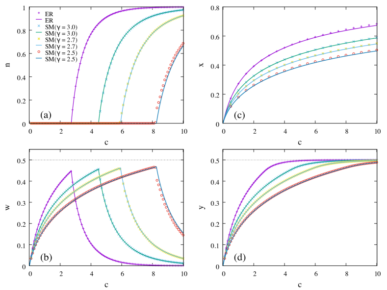
Figure 2: The fractions of core vertices $n$ and roots $w$ from the GLR procedure, the MVC fraction $x$, and the MM fraction $y$ on the Erdös-Rényi (ER) random graphs and the scale-free networks generated with the static model (SM) with a degree exponent $\gamma=3.0,2.7,2.5$. In (c), each sign is a result of the hybrid (GLR+BPD) algorithm on a single graph instance with a vertex size $N=10^{5}$; elsewhere, each sign is a simulation result on a single graph instance with a vertex size $N=10^{6}$. Each solid line is a mean-field prediction on infinitely large graphs.

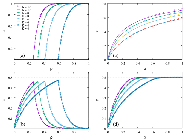
Figure 3: The fractions of core vertices $n$ and roots $w$ from the GLR procedure, the MVC fraction $x$, and the MM fraction $y$ on the diluted regular random (dRR) graphs with an initial degree $K=10,8,6,4$. In (c), each sign is a result of the hybrid (GLR+BPD) algorithm on a single diluted graph instance with a vertex size $N=10^{5}$; elsewhere, each sign is a simulation result averaged on $40$ independently generated graph instances with a vertex size $N=10^{5}$, with which the standard deviation for each data point is also shown. Each solid line is a mean-field prediction on infinitely large graphs.

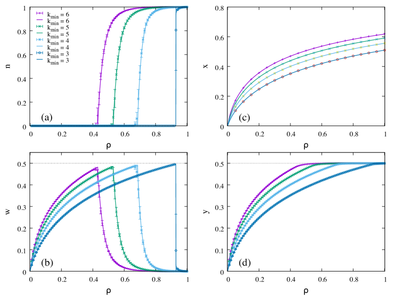
Figure 4: The fractions of core vertices $n$ and roots $w$ from the GLR procedure, the MVC fraction $x$, and the MM fraction $y$ on the diluted instances from a scale-free (SF) network generated with the configurational model with a vertex size $N=10^{5}$, a degree exponent $\gamma=2.5$, a maximal degree $k_{\rm{max}}=\sqrt{N}$, and a minimal degree $k_{\rm{min}}=6,5,4,3$. In (c), each sign is a result of the hybrid (GLR+BPD) algorithm on a single diluted instance of the SF network; elsewhere, each sign is a simulation result averaged on $40$ independently generated diluted instances of the SF network, with which the standard deviation for each data point is also shown. Each solid line is a mean-field prediction with the empirical degree distribution of the SF network as input.

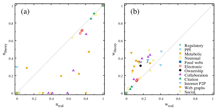
Figure 5: The fractions of core vertices $n$ and roots $w$ from the GLR procedure on real-world network instances. The fractions $n_{\rm{real}}$ and $w_{\rm{real}}$ are directly read from the GLR procedure on the network instances. The fractions $n_{\rm{theory}}$ and $w_{\rm{theory}}$ are the mean-field predictions with the empirical degree distribution of each network instance as input. Data points are grouped by network categories.

Here we apply our frameworks for the GLR procedure, the MVCs, and the MMs on some model random graphs and real-world networks. Details for graph construction and equations for random graph models are left in appendix C. A brief description of the real-world network dataset is left in appendix D.

An Erdös-Rényi (ER) random graph Erdos.Renyi-PublMath-1959 ; Erdos.Renyi-Hungary-1960 with a mean degree $c$ has a Poisson degree distribution as $P(k)=e^{-c}c^{k}/k!$. Results of simulation and analytical theory of the GLR procedure are in figure 2. There are two regimes in which $n$ and $w$ follow consistent scenarios respectively, separated by the core birth point Bauer.Golinelli-EPJB-2001 ; Liu.Csoka.Zhou.Posfai-PRL-2012 . In the coreless regime $c<e\approx 2.71828$, we have $1-\alpha-\beta=0$, $n=0$, and $w$ continuously increasing from $0$ to a maximum $w^{\star}\approx 0.44816$. In the core regime $c>e$, we have $1-\alpha-\beta>0$, $n$ continuously increasing from $0$, and $w$ continuously decreasing from $w^{\star}$. Here we present an intuitive understanding of these regimes. When $c$ is rather small, a graph is simply a collection of trees and has no macroscopic GCC Molloy.Reed-RandStructAlgo-1995 . The GLR procedure can remove all edges with few generated leaves. After the GCC forms and with the initial leaf size ($P(1)$) decreasing, the iterative GLR procedure relies more and more on generated leaves. Yet due to the relative low density of edges in the graph, the GLR procedure can still remove all edges, resulting in a trivial $n$. Meanwhile more single GLR steps are needed with an increasing $c$, leading to an increasing root size $w$. After a core forms ($c>e$) and with more edges added, the initial leaf size further decreases. More severely, new leaves are difficult to generate in the procedure due to the increasing density of edges. Thus in general the size of GLR steps decreases, leading to both an increasing $n$ and a decreasing $w$, trending as $n\rightarrow 1$ and $w\rightarrow 0$ at the same time. We will see that this picture holds for other model random graphs.

We consider the MVCs on ER random graphs. On the ER random graphs without cores ($c\leq e$), the MVC sizes have been derived exactly with a numeration method for the GLR procedure (basically a discrete approach to the core percolation theory) Karp.Sipser-IEEFoCS-1981 ; Bauer.Golinelli-EPJB-2001 . On general ER random graphs, the MVC sizes are estimated by the replica symmetric calculation at zero temperature Weigt.Hartmann-PRL-2000 and the cavity method based on the long-range frustration among MVC solutions Zhou-PRL-2005 , both of which reduce to the exact results in the regime of graphs without cores and serve as an approximation on graphs with cores. The well-known replica symmetric result in Weigt.Hartmann-PRL-2000 states that the MVC fractions follow

$$\hat{x}=1-\frac{1}{2c}(2W(c)+W(c)^{2}),$$ (15)

in which $W(c)$ is the Lambert-W-function as $W(c)e^{W(c)}=c$. From our framework and equations in appendix C, we have

$$x=1-e^{-c\alpha}-\frac{1}{2}c\alpha^{2},\ \textrm{s.t.}\ 1-\alpha-\beta=0,$$ (16)

in which $\alpha$ and $\beta$ are calculated from equations (44) and (45). Here we prove that our framework simply retrieves equation (15). We define two auxiliary functions as $A\equiv ce^{-c\alpha}$ and $B\equiv c\alpha$, thus we have $x=1-(2A+B^{2})/2c$. A list of equivalence can be carried out as

$$A \equiv ce^{-c\alpha}=ce^{-c(1-\beta)}=c\alpha\equiv B,$$ (17)

$$Be^{B} \equiv c\alpha e^{c\alpha}=ce^{-c(1-\beta)}e^{c\alpha}=ce^{-c(1-\alpha-\beta)}=c,$$ (18)

employing only the trivial core condition and equation (44). Thus $A=B=W(c)$, proving that $x$ and $\hat{x}$ are the same. This equivalence shows that, the trivial unstable branch of fixed solutions for a percolation problem, which is largely neglected in the present percolation study, indeed has a physical interpretation, which is closely related to a replica symmetric result of the underlying optimization problems.

We also consider the MMs on ER random graphs. An enumeration method for the GLR procedure Karp.Sipser-IEEFoCS-1981 ; Bauer.Golinelli-EPJB-2001 and the cavity method at the first replica symmetric breaking (1RSB) level Zhou.OuYang-arxiv-2003 both estimate the MM fraction as

$$\hat{y}=\frac{1}{2}(1-\alpha+\beta-c\alpha+c\alpha\beta),$$ (19)

in which $\alpha$ and $\beta$ are derived from $\alpha=e^{-ce^{-c\alpha}},\beta=1-e^{-c\alpha}$. Here we prove that our framework simply retrieves equation (19). First, it is easy to see that the two iterative equations for equation (19) are just equations (44) and (45). Then, after we simplify equation (14) with Poisson degree distributions and remove the exponential terms with equation (44) and (45), we finally have equation (19).

We also consider our framework on the diluted regular random (dRR) graphs. A dRR graph is obtained by an edge dilution scheme on a regular random (RR) graph with a uniform integer degree $K$ ($\geq 2$) for each vertex, in which a fraction $1-\rho\in[0,1]$ of edges is randomly chosen and removed. Results are shown in figure 3.

We further consider the scale-free (SF) networks Barabasi.Albert-Science-1999 with a power-law degree distribution $P(k)\propto k^{-\gamma}$ with a degree exponent $\gamma$. There are several models to generate SF network instances. First we consider the configurational model Newman.Strogatz.Watts-PRE-2001 ; Zhou.Lipowsky-PNAS-2005 , which generates a graph instance directly from its empirical degree distribution. Results on diluted SF networks with $\gamma=2.5$ are in shown figure 4. Theory and simulation correspond very well except those results of $n$ and $w$ close to core birth. An explanation is the finite-size effect at the phase transition points on the relatively small graph instances. We then consider the asymptotical SF networks generated with the static model Goh.Kahng.Kim-PRL-2001 ; Catanzaro.PastorSatorras-EPJB-2009 . Results are shown in figure 2. For $n$ and $w$, a discernible discrepancy sets in with small $\gamma$. It has been analytically proved Goh.Kahng.Kim-PRL-2001 ; Catanzaro.PastorSatorras-EPJB-2009 that the SF networks generated with the static model with $\gamma>3$ behave more like ER random graphs with $\gamma$ increasing, while those with $\gamma<3$ show more significant degree-degree correlation with $\gamma$ decreasing. Besides the degree-degree correlation in the SF networks with $\gamma<3$, the loop structure is also a contributing factor to the deviation of the mean-field results. An analytical discussion of finite size correction through loops can be found in Lucibello.etal-PRE-2014 .

We also test the GLR procedure on real-world networks. Results from simulation and theory are shown in figure 5. For most data points, we can see two straight-forward tendencies. The first one is that the discrepancies between simulation and theoretical results show a negative tendency. It is easy to understand, because cores and roots are much like complementary structure of a graph. The second tendency is that large discrepancies between simulation and theory exist among most of the network instances. It shows a fundamental limitation of the basis of our analytical theory, the local tree-structure assumption Mezard.Montanari-2009 . Real networks show rich mesoscopic and higher-order structures at various scales, such as the degree-degree correlation among neighboring vertices Newman-PRL-2002 , the community structure and the modularity Newman-NatPhys-2012 , and the hierarchical organizations CorominasMurtra.etal-PNAS-2013 . All these factors can be slimly captured by the degree distribution, which is the only information of graph structure into our mean-field theory, thus can fail the analytical prediction.

V Conclusion

The geometrical implication of roots and cores from the GLR procedure in the MVC and the MM problems has long been formulated in an algorithmic sense, yet on the analytical side a thorough exploration is still missing except the mean-field theory of core emergence. In this paper, by completing the missing theory of roots from the GLR procedure, we develop a unified framework to estimate MVC and MM sizes on random graphs with or without cores: with the branch of trivial fixed solutions of the iterative cavity equations of the GLR procedure, we derive the zero-temperature replica symmetric solution of the MVC fractions; with the branch of stable fixed solutions, we reproduce the zero-temperature replica symmetric estimation of the MM fractions. Our frameworks are built on a geometrical interpretation of roots and cores, which makes them different from the typical formulation of optimization problems into statistical physical systems with zero or finite temperatures. Besides, our frameworks have a simple and easily interpretable form, without involving complicated statistical physical tricks.

There are still points deserving further exploration, particularly the physical interpretation of the unstable branch of self-consistent equations common in mean-field theories for random systems. A recent study Zhou-PRL-2019 in the Bethe-Peierls mean-field theory for the $Q$-state Potts model on random graphs discusses the physical role of the middle unstable branch of cavity probabilities in the microcanonical discontinuous phase transitions.

VI Acknowledgements

This work is supported by the National Natural Science Foundation of China (Grant Nos. 11421063 and 11747601) and the Chinese Academy of Sciences (Grant No. QYZDJ-SSW-SYS018). J-H Zhao is supported partially by the Key Research Program of Frontier Sciences of the Chinese Academy of Sciences (Grant No. QYZDB-SSW-SYS032) and the National Natural Science Foundation of China (Grant No. 11605288). J-H Zhao thanks Prof. Pan Zhang (ITP-CAS) for his hospitality.

VII Appendix A: A discrete theoretical formulation of the GLR procedure

VII.1 A discrete form of $\alpha$ and $\beta$

We consider the discretized GLR procedure on an undirected graph $G=\{V,E\}$. At each $t$-th time-step with a discrete index $t\geq 0$, all leaves and their roots are determined, and their adjacent edges are removed. Beware that a ’time-step’ of GLR procedure here usually involves multiple ’single steps’ of the GLR procedure in which only one root is removed at a step. We can calculate the pertinent quantities just after each $t$-th time-step. In the case of infinite time steps as $t\rightarrow\infty$, the discretized GLR procedure is iterated until there is no leaf left. Correspondingly, the residual subgraph constitutes the core, and the roots can be counted by summing those removed during all the time-steps.

Following a similar logic of the definition of $\alpha$ and $\beta$ in equations (1) and (2), we define cavity probabilities $\alpha^{(t)}$ and $\beta^{(t)}$ for the $t$-th time-step ($t\geq 0$). With a randomly chosen edge $(i,j)\in G$ and following the vertex $i$ to the vertex $j$, we define $\alpha^{(t)}$ ($\beta^{(t)}$) as the probability that $j$ becomes a leaf (a root) at exactly the $t$-th time-step on $G\backslash(i,j)$. We also define the cumulative cavity probabilities $\alpha^{(c,t)}\equiv\sum_{t^{\prime}=0}^{t}\alpha^{(t^{\prime})}$ ($\beta^{(c,t)}\equiv\sum_{t^{\prime}=0}^{t}\beta^{(t^{\prime})}$) as the probability that $j$ becomes a leaf (a root) before or at the $t$-th time-step on $G\backslash(i,j)$. We then derive the iterative equations of $\alpha^{(t)}$ and $\beta^{(t)}$ with $t\geq 0$ based on the local tree-structure approximation on sparse random graphs.

$$\alpha^{(t)} =\left\{\begin{array}[]{lcr}Q(1),&\mbox{for}&t=0;\\ \sum_{k=1}^{\infty}Q(k)(\beta^{(c,0)})^{k-1}-Q(1),&\mbox{for}&t=1;\\ \sum_{k=1}^{\infty}Q(k)[(\beta^{(c,t-1)})^{k-1}-(\beta^{(c,t-2)})^{k-1}],&\mbox{for}&t\geq 2;\end{array}\right.$$ (23)

$$\beta^{(t)} =\left\{\begin{array}[]{lcr}\sum_{k=1}^{\infty}Q(k)[1-(1-\alpha^{(c,0)})^{k-1}],&\mbox{for}&t=0;\\ \sum_{k=1}^{\infty}Q(k)\{[1-(1-\alpha^{(c,t)})^{k-1}]-[1-(1-\alpha^{(c,t-1)})^{k-1}]\},&\mbox{for}&t\geq 1.\end{array}\right.$$ (26)

Here is an explanation for the equations. With a randomly chosen edge $(i,j)\in G$, we consider the state of $j$ from a cavity graph $G\backslash j$ to another cavity graph $G\backslash(i,j)$ at the $t$-th time-step under the GLR procedure after the corresponding edge addition. For $\alpha^{(t)}$, if the vertex $j$ becomes a leaf at the $t$-th time-step on $G\backslash(i,j)$, all the nearest neighbors of $j$ except $i$ should all be removed as roots before or at the $(t-1)$-th time-step on $G\backslash j$, among which there should be at least one nearest neighbors being roots at the $(t-1)$-th time-step. For $\beta^{(t)}$, if the vertex $j$ becomes a root at the $t$-th time-step on $G\backslash(i,j)$, among the nearest neighbors of $j$ except $i$ there should be at least one nearest neighbors being leaves before or at the $t$-th time-step on $G\backslash j$, among which there should be at least one nearest neighbors being leaves at the $t$-th time-step.

We can further derive iterative equations for $\alpha^{(c,t)}$ and $\beta^{(c,t)}$ with $t\geq 0$. For $\alpha^{(c,t)}$, it’s simple to verify that $\alpha^{(c,0)}\equiv\alpha^{(0)}=Q(1)$, and $\alpha^{(c,1)}\equiv\alpha^{(0)}+\alpha^{(1)}=\sum_{k=1}^{\infty}Q(k)(\beta^{(c,0)})^{k-1}$. For $t\geq 2$, we have

$$\alpha^{(c,t)} \equiv\alpha^{(c,1)}+\alpha^{(2)}+...+\alpha^{(t)}$$

$$=\alpha^{(c,1)}+\sum_{k=1}^{\infty}Q(k)(\beta^{(c,1)})^{k-1}-\sum_{k=1}^{\infty}Q(k)(\beta^{(c,0)})^{k-1}+...$$

$$+\sum_{k=1}^{\infty}Q(k)(\beta^{(c,t-1)})^{k-1}-\sum_{k=1}^{\infty}Q(k)(\beta^{(c,t-2)})^{k-1}$$

$$=\sum_{k=1}^{\infty}Q(k)(\beta^{(c,t-1)})^{k-1}.$$

We can see that the above equation also holds for $t=1$. For $\beta^{(c,t)}$, we have $\beta^{(c,0)}\equiv\beta^{(0)}$. With $t\geq 1$, we have

$$\beta^{(c,t)} \equiv\beta^{(0)}+\beta^{(1)}+...+\beta^{(t)}$$

$$=\beta^{(0)}+\sum_{k=1}^{\infty}Q(k)[1-(1-\alpha^{(c,1)})^{k-1}]-\sum_{k=1}^{\infty}Q(k)[1-(1-\alpha^{(c,0)})^{k-1}]+...$$

$$+\sum_{k=1}^{\infty}Q(k)[1-(1-\alpha^{(c,t)})^{k-1}]-\sum_{k=1}^{\infty}Q(k)[1-(1-\alpha^{(c,t-1)})^{k-1}]$$

$$=\sum_{k=1}^{\infty}Q(k)[1-(1-\alpha^{(c,t)})^{k-1}].$$

The above equation also holds for $t=0$.

Summing the above results, $\alpha^{(c,t)}$ and $\beta^{(c,t)}$ with $t\geq 0$ can be derived from the initial condition $\alpha^{(c,0)}=Q(1)$ and the updating equations

$$\alpha^{(c,t)} =\sum_{k=1}^{\infty}Q(k)(\beta^{(c,t-1)})^{k-1},$$ (27)

$$\beta^{(c,t)} =1-\sum_{k=1}^{\infty}Q(k)(1-\alpha^{(c,t)})^{k-1}.$$ (28)

We present a numerical method to calculate the cavity probabilities $(\alpha^{(c,t)},\beta^{(c,t)})$, thus $(\alpha^{(t)},\beta^{(t)})$, with any $t\geq 0$. With the initial condition $\alpha^{(c,0)}=Q(1)$, we can derive $\beta^{(c,0)}$ with equation (28), thus we have $(\alpha^{(c,0)},\beta^{(c,0)})$. With any cavity probability $(\alpha^{(c,t^{\prime})},\beta^{(c,t^{\prime})})$ with $t^{\prime}\geq 0$, we can calculate $\alpha^{(c,t^{\prime}+1)}$ with equation (27) and $\beta^{(c,t^{\prime}+1)}$ with equation (28), thus we have $(\alpha^{(c,t^{\prime}+1)},\beta^{(c,t^{\prime}+1)})$. In such a progressive process, we can calculate $(\alpha^{(c,t)},\beta^{(c,t)})$ with any $t\geq 0$. To stop the probability updating as $(\alpha^{(c,t)},\beta^{(c,t)})$ converges at large $t$, we can set a simple criterion: we terminate at the $T$-th step once $|\alpha^{(c,T)}-\alpha^{(c,T-1)}|+|\beta^{(c,T)}-\beta^{(c,T-1)}|<\epsilon$, in which $\epsilon$ is a small positive number such as $\epsilon=10^{-8}$.

VII.2 A discrete form of $n$, $l$, and $w$

Here we calculate some quantities just after the $t$-th time-step of the discretized GLR procedure. In this context, the relative sizes of vertices and edges in the residual subgraph and the accumulated removed roots (all normalized by the vertex size) are denoted as $n^{(c,t)}$, $l^{(c,t)}$, and $w^{(c,t)}$ with $t\geq 0$, respectively.

For $n^{(c,t)}$, it can be written down as

$$n^{(c,t)} =\sum_{k=2}^{\infty}P(k)\sum_{s=2}^{k}\left(\begin{array}[]{c}k\\ s\end{array}\right)(\beta^{(c,t)})^{k-s}(1-\alpha^{(c,t)}-\beta^{(c,t)})^{s}.$$ (31)

Here is a simple explanation. With a randomly chosen vertex $i$, we move from a cavity graph $G\backslash i$ to the original graph $G$ after some edge addition. If $i$ is in the residual subgraph of $G$ just after the $t$-th time-step, on $G\backslash i$ it should have: (1) no nearest neighbor turning into a leaf before or at the $t$-th time-step; (2) at least two nearest neighbors which are also in the residual subgraph just after the $t$-th time-step; and (3) all the other nearest neighbors becoming roots before or at the $t$-th time-step.

For $l^{(c,t)}$, we have

$$l^{(c,t)} =\frac{1}{2}c(1-\alpha^{(c,t)}-\beta^{(c,t)})^{2}.$$ (32)

Here is a simple explanation. We move from a cavity graph $G\backslash(i,j)$ to $G$ as $(i,j)\in G$ is a randomly chosen edge. If $(i,j)$ is in the residual graph of $G$ just after the $t$-th time-step, both its end-vertices should be in the residual graph of $G\backslash(i,j)$ just after the $t$-th time-step, thus we have the squared term. The multiplicative factor $c/2(=|E|/|V|)$ is the relative size of edges to vertices.

For $w^{(c,t)}$, we follow a similar calculation in the context of a generalized GLR procedure for the minimum dominating set problem Zhao.Zhou-JStatPhys-2015 ; Zhao.Zhou-LNCS-2015 . For the GLR procedure here, we have

$$w^{(c,t)} =\frac{1}{2}P(1)Q(1)+\sum_{k=2}^{\infty}P(k)[1-(1-\alpha^{(c,t)})^{k}]$$ (33)

$$-\frac{1}{2}\sum_{k=2}^{\infty}P(k)k\alpha^{(1)}(\beta^{(0)})^{k-1}$$

$$-\frac{1}{2}\sum_{\tau=2}^{t}\sum_{k=2}^{\infty}P(k)k\alpha^{(\tau)}[(\beta^{(c,\tau-1)})^{k-1}-(\beta^{(c,\tau-2)})^{k-1}]$$

$$-\sum_{\tau=1}^{t-1}\sum_{k=2}^{\infty}P(k)k\alpha^{(\tau+1)}(\beta^{(c,\tau-1)})^{k-1}.$$

Here is a simple explanation. (1) The first term counts the isolated edge with both end-vertices as leaves. (2) The second term is a summation of the possibilities that a random vertex, say $i$, having some nearest neighbor being leaves before or at the $t$-th time-step on the cavity graph $G\backslash i$. Yet there are recounting terms from the newly generated isolated edges and terms contradicting the pruning process of the discretized GLR procedure, which are further subtracted in the following three terms. (3) - (4) The recounting case happens when a certain edge turns out to be an isolated edge on $G$ at certain time step. Specifically, at the $\tau$-th $(1\leq\tau\leq t)$ time-step of the GLR procedure on $G\backslash j$, if all the nearest neighbors of $j$ except $i$ are pruned already as roots before or at the $(\tau-1)$-th time-step among which some nearest neighbors are pruned at exactly the $(\tau-1)$-th time-step, $j$ will become a leaf at the $\tau$-th time-step on $G\backslash(i,j)$. If $i$ happens to be a leaf at the $\tau$-th time-step on $G\backslash(i,j)$, an isolated edge $(i,j)$ emerges on $G$. The third and fourth terms sums these probabilities of the case of $\tau=1$ and $2\leq\tau\leq t$ respectively. (5) The fifth term deals with the contradiction case when a product of cavity probabilities from the second term does not correspond to a proper state transition in the discretized GLR procedure. At the $\tau$-th time-step ($1\leq\tau\leq t-1$) of the GLR procedure on $G\backslash j$, if all the nearest neighbors of $j$ except $i$ are pruned as roots before or at the $(\tau-1)$-th time-step, $j$ will be a leaf before or at the $\tau$-th time-step on $G\backslash(i,j)$. A contradiction happens when $i$ turns into a leaf at the $(\tau+1)$-th time-step on $G\backslash(i,j)$. The reason is that, in a proper scenario, $i$ should be a leaf or simply a root at the $\tau$-th time-step on $G\backslash(i,j)$, thus the states of $i$ and $j$ can be well defined in $G$.

Below we further simplify $w^{(c,t)}$. On the RHS of equation (33), in the second term we reformulate $\sum_{k=2}^{\infty}$ with $\sum_{k=0}^{\infty}$, in the fifth term we change from $\sum_{\tau=1}^{t-1}$ to $\sum_{\tau=2}^{t}$, and we further combine the fourth and the fifth terms. We also see $\alpha^{(0)}=Q(1)$. We then have

$$w^{(c,t)} =\frac{1}{2}P(1)\alpha^{(0)}+\sum_{k=0}^{\infty}P(k)[1-(1-\alpha^{(c,t)})^{k}]-P(1)\alpha^{(c,t)}$$

$$-\frac{1}{2}\sum_{k=2}^{\infty}P(k)k\alpha^{(1)}(\beta^{(0)})^{k-1}$$

$$-\frac{1}{2}\sum_{\tau=2}^{t}\sum_{k=2}^{\infty}P(k)k\alpha^{(\tau)}[(\beta^{(c,\tau-1)})^{k-1}+(\beta^{(c,\tau-2)})^{k-1}].$$

We further move from $\sum_{k=2}^{\infty}$ to $\sum_{k=1}^{\infty}$ in the last two terms, and rearrange the equation.

$$w^{(c,t)} =\sum_{k=0}^{\infty}P(k)[1-(1-\alpha^{(c,t)})^{k}]+\frac{1}{2}P(1)\alpha^{(0)}-P(1)\alpha^{(c,t)}$$

$$-\frac{1}{2}\sum_{k=1}^{\infty}P(k)k\alpha^{(1)}(\beta^{(0)})^{k-1}+\frac{1}{2}P(1)\alpha^{(1)}$$

$$-\frac{1}{2}\sum_{\tau=2}^{t}\sum_{k=1}^{\infty}P(k)k\alpha^{(\tau)}[(\beta^{(c,\tau-1)})^{k-1}+(\beta^{(c,\tau-2)})^{k-1}]$$

$$+\frac{1}{2}\sum_{\tau=2}^{t}P(1)\alpha^{(\tau)}[1+1].$$

We combine all the non-summation terms with $P(1)$, and further adopt the equivalence $cQ(k)=kP(k)$. We have

$$w^{(c,t)} =\sum_{k=0}^{\infty}P(k)[1-(1-\alpha^{(c,t)})^{k}]-\frac{1}{2}cQ(1)\alpha^{(c,1)}$$

$$-\frac{1}{2}\sum_{k=1}^{\infty}cQ(k)\alpha^{(1)}(\beta^{(0)})^{k-1}$$

$$-\frac{1}{2}\sum_{\tau=2}^{t}\sum_{k=1}^{\infty}cQ(k)\alpha^{(\tau)}[(\beta^{(c,\tau-1)})^{k-1}+(\beta^{(c,\tau-2)})^{k-1}].$$

Considering the equivalence $\alpha^{(0)}=Q(1)$ for the second term and equation (27) for the last two terms, we have

$$w^{(c,t)} =\sum_{k=0}^{\infty}P(k)[1-(1-\alpha^{(c,t)})^{k}]-\frac{1}{2}c\alpha^{(0)}\alpha^{(c,1)}$$

$$-\frac{1}{2}c\alpha^{(1)}\alpha^{(c,1)}-\frac{1}{2}\sum_{\tau=2}^{t}c\alpha^{(\tau)}[\alpha^{(c,\tau)}+\alpha^{(c,\tau-1)}].$$

Combining the second and third terms as $\alpha^{(c,1)}\equiv\alpha^{(0)}+\alpha^{(1)}$, and considering the definition $\alpha^{(t)}\equiv\alpha^{(c,t)}-\alpha^{(c,t-1)}$, we have

$$w^{(c,t)} =\sum_{k=0}^{\infty}P(k)[1-(1-\alpha^{(c,t)})^{k}]-\frac{1}{2}c(\alpha^{(c,1)})^{2}$$

$$-\frac{1}{2}\sum_{\tau=2}^{t}c[(\alpha^{(c,\tau)})^{2}-(\alpha^{(c,\tau-1)})^{2}].$$

Expanding the third term, we finally have

$$w^{(c,t)}=1-\sum_{k=0}^{\infty}P(k)(1-\alpha^{(c,t)})^{k}-\frac{1}{2}c(\alpha^{(c,t)})^{2}.$$ (34)

VII.3 At infinite time-steps

When $t\rightarrow\infty$, the discrete description corresponds to the termination of the GLR procedure on graphs. The solution $(\alpha^{(c,\infty)},\beta^{(c,\infty)})$ can be derived as the convergent values of equations (27) and (28), with which we can calculate $n^{(c,\infty)}$, $l^{(c,\infty)}$, and $w^{(c,\infty)}$. In another word, $\alpha^{(c,\infty)}$, $\beta^{(c,\infty)}$, $n^{(c,\infty)}$, $l^{(c,\infty)}$, and $w^{(c,\infty)}$ reduce respectively to $\alpha$, $\beta$, $n$, $l$, and $w$ in the main text.

VIII Appendix B: Belief propagation algorithms for the MVC problem

Here we discuss briefly how the MVC problem can be mapped to a statistical physical system and its approximate mean-field message-passing algorithms in the replica symmetric regime, such as the belief propagation (BP) algorithm and belief propagation-guided decimation (BPD) algorithm. More detailed discussions on message-passing algorithms can be found in Weigt.Zhou-PRE-2006 ; Zhang.Zeng.Zhou-PRE-2009 .

The MVC problem, an optimization problem in nature, can be considered as a statistical physical system, in which its optimum corresponds to the (zero-temperature) ground-state energy of the corresponding physical formulation. We discuss the problem in the context of an undirected graph $G=\{V,E\}$ with a vertex set $V$ and an edge set $E$. For each vertex, say $i\in V$, a covering state can be assigned as $s_{i}=1(0)$ as the vertex being in (not in) a MVC. A covering state for $G$ can be denoted as a vector $\vec{s}\equiv(s_{1},...,s_{|V|})$. The energy $E(\vec{s})$ for a covering state $\vec{s}$ is simply $E(\vec{s})=\sum_{i\in V}s_{i}$. For the physical system on $G$ with a finite inverse temperature $x$, the partition function is

$$Z(x)=\sum_{\vec{s}}\prod_{i\in V}e^{-xs_{i}}\prod_{(j,k)\in E}[1-(1-s_{j})(1-s_{k})].$$ (35)

In the equation, the summation runs on all the $2^{|V|}$ possible covering state configurations, the first product counts all the reweighting Boltzmann factors for a covering state, and the second product selects any covering state as a proper VC under the topological constraint. In all, only VC configurations among all the possible covering states contribute to the partition function of the physical system. From the partition function, the thermal quantities of the physical system can de derived with standard statistical physical methods. In the case of $x\rightarrow\infty$, only those VC configurations with the smallest cardinality are considered, thus evaluating equation (35) reduces to the MVC problem.

Calculating equation (35) analytically is extremely difficult, and the mean-field theoretical methods, such as the replica trick and the cavity method from the spin glass theory, are adopted. The BP algorithm of the cavity method is based on the assumption of locally tree-like structure on sparse random graphs, and works in the replica symmetric regime, in which all the solutions are assumed to be organized in a macroscopic state. On any edge $(i,j)\in G$ from the vertex $i$ to the vertex $j$, we define the cavity probability (or cavity message) $p_{i\rightarrow j}$ as the probability of $i$ to be in a MVC on the cavity graph $G\backslash(i,j)$. We can see that there are in total $2|E|$ cavity probabilities for $G$. For any vertex $i\in G$, we define the marginal probability $p_{i}$ as the probability of $i$ to be in a MVC on $G$. Here we consider the case from a cavity graph $G\backslash i$ to $G$. If the vertex $i$ is in a MVC, a Boltzmann factor $e^{-x}$ is introduced; otherwise, the probability of $i$ to be not in a MVC is $\prod_{k\in\partial i}p_{k\rightarrow i}$. Thus we have the formulation of marginal probabilities based on the cavity probabilities as

$$p_{i}=\frac{e^{-x}}{e^{-x}+\prod_{k\in\partial i}p_{k\rightarrow i}}.$$ (36)

Following the above logic, in the case from $G\backslash i$ to $G\backslash(i,j)$, we have the self-consistent equation for cavity probabilities as

$$p_{i\rightarrow j}=\frac{e^{-x}}{e^{-x}+\prod_{k\in\partial i\backslash j}p_{k\rightarrow i}},$$ (37)

in which $\partial i\backslash j$ is the set of the nearest neighbors of $i$ excluding $j$. With the fixed point of the $2|E|$ self-consistent equations of cavity probabilities on $G$ with equation (37), the thermal properties of the statistical physical system can be estimated. The energy density or the fraction $e$ of the MVCs is estimated as the averaged marginal probability of any vertex. We have

$$e=\frac{1}{|V|}\sum_{i\in V}p_{i}=\frac{1}{|V|}\sum_{i\in V}\frac{e^{-x}}{e^{-x}+\prod_{j\in\partial i}p_{j\rightarrow i}}.$$ (38)

The free energy of the physical system is summed from the free energy perturbations of adding a vertex or an edge to the corresponding cavity graph. We have the free energy density

$$f=\frac{1}{|V|}(\sum_{i\in V}\Delta F_{i}-\sum_{(i,j)\in E}\Delta F_{(i,j)}),$$ (39)

in which $\Delta F_{i}$ for any vertex $i\in V$ is the free energy contribution by adding $i$ into the cavity graph $G\backslash i$, and $\Delta F_{(i,j)}$ for any edge $(i,j)\in E$ is the free energy contribution by adding $(i,j)$ into the cavity graph $G\backslash(i,j)$. We have

$$\Delta F_{i} =-\frac{1}{x}\ln(e^{-x}+\prod_{j\in\partial i}p_{j\rightarrow i}),$$ (40)

$$\Delta F_{(i,j)} =-\frac{1}{x}\ln[1-(1-p_{i\rightarrow j})(1-p_{j\rightarrow i})].$$ (41)

Thus we have the entropy density as $s=x(e-f)$.

The BP algorithm estimates the average physical properties in a ensemble sense, yet the BPD algorithm applies on graph instances and approximates solution configurations. Basically, the BPD algorithm guides the searching for approximate solutions by fixing into certain states those vertices or edges with the most biased marginal probabilities in an iterative graph simplification process. The component of the BPD algorithm in the hybrid algorithm of the main text goes as: (1) the cavity probabilities are initialized randomly $\in(0,1)$ on each edge of the current core of the residual graph from the GLR procedure; (2) all the cavity probabilities are updated following equation (37) until a given maximal sweep size $N_{\rm{up}}$ or a convergence of cavity probabilities under some criterion; (3) the marginal probability for each vertex is calculated with equation (36); (4) in a single decimation step, a small size $N_{\rm{d}}$ of the vertices in the core with the largest marginal probabilities are selected into a VC and are further removed along with their adjacent edges. For the convergence criterion to terminate the probability updating at the $T$-th ($T\geq 1$) sweep, we set for convenience $\max_{(i,j)\in E}|p_{i\rightarrow j}^{(T)}-p_{i\rightarrow j}^{(T-1)}|<\epsilon$, in which $p_{i\rightarrow j}^{(T)}$ is the value of $p_{i\rightarrow j}$ at the $T$-th sweep of the probability updating and the positive parameter $\epsilon\ll 1$. For the size of removed vertices in a single decimation step, we set $N_{\rm{d}}=\max\{N_{\rm{core}}/f_{\rm{d}},N_{\rm{dmin}}\}$, in which $N_{\rm{core}}$ is the vertex size of the current core, $f_{\rm{d}}$ as a fraction coeffiecient, and $N_{\rm{dmin}}$ as the smallest size of vertices to be removed. In choosing a proper inverse temperature $x$ for the BPD algorithm, we set $x$ as its largest value at which the corresponding entropy density $s$ vanishes.

In the main text, we set $x=10.0$, $N_{\rm{up}}=200$, $\epsilon=10^{-8}$, $f_{\rm{d}}=200$, and $N_{\rm{dmin}}=1$. Beware that, by tuning $x$ adaptively for specific graph ensembles, increasing $N_{\rm{up}}$ and $f_{\rm{d}}$, and decreasing $\epsilon$, we can improve results from the BPD algorithm.

IX Appendix C: Equations for the GLR procedure on random graphs

IX.1 Erdös-Rényi random graphs

An ER random graph instance with a vertex size $N$ and a mean degree $c$ can be constructed by adding $M(\equiv cN/2)$ edges to an empty graph with only $N$ vertices by connecting pairs of randomly chosen distinct vertices.

On ER random graphs, we have the degree distributions as

$$P(k) =e^{-c}\frac{c^{k}}{k!},$$ (42)

$$Q(k) =e^{-c}\frac{c^{k-1}}{(k-1)!}.$$ (43)

We have simplified equations as

$$\alpha =e^{-c(1-\beta)},$$ (44)

$$\beta =1-e^{-c\alpha},$$ (45)

$$n =e^{-c\alpha}-e^{-c(1-\beta)}-c\alpha(1-\alpha-\beta),$$ (46)

$$w =1-e^{-c\alpha}-\frac{1}{2}c\alpha^{2}.$$ (47)

IX.2 Regular random graphs

For dRR graphs after an edge dilution scheme with a parameter $\rho$ on RR graphs with an original degree $K$, we have degree distributions

$$P(k) =\left(\begin{array}[]{c}K\\ k\end{array}\right)\rho^{k}(1-\rho)^{K-k},$$ (50)

$$Q(k) =\left(\begin{array}[]{c}K-1\\ k-1\end{array}\right)\rho^{k-1}(1-\rho)^{K-k}.$$ (53)

We further have simplified equations as

$$\alpha =(1-\rho(1-\beta))^{K-1},$$ (54)

$$\beta =1-(1-\rho\alpha)^{K-1},$$ (55)

$$n =(1-\rho\alpha)^{K}-(1-\rho(1-\beta))^{K}-\rho K\alpha(1-\alpha-\beta),$$ (56)

$$w =1-(1-\rho\alpha)^{K}-\frac{1}{2}\rho K\alpha^{2}.$$ (57)

IX.3 Scale-free networks with the configurational model

First we show how to construct scale-free (SF) networks with the configurational model. The key graph parameters here are: $N$ the vertex size, $\gamma$ the degree exponent, $k_{\rm{min}}$ the minimal degree, and $k_{\rm{max}}$ the maximal degree. For simplicity, in this paper we set $k_{\rm{min}}\geq 2$ and $k_{\rm{max}}=\sqrt{N}$. The graph generation is as follows. (1) A sequence of degrees is generated with $N(k)=NP_{0}(k)$ with $k_{\rm{min}}\leq k\leq k_{\rm{max}}$ and $P_{0}(k)=k^{-\gamma}/\sum_{m=k_{\rm{min}}}^{k_{\rm{max}}}m^{-\gamma}$. Thus we have a size of free studs (half-edges) $E=\sum_{k=k_{\rm{min}}}^{k_{\rm{max}}}kN(k)$. (2) For any vertex $i$, we assign its degree $k_{i}$ sampled from the distribution $N(k)$. Thus we have an empty graph configuration with $N$ vertices while any vertex $i$ has $k_{i}$ free studs. If $E$ is odd, we can randomly chose a vertex $i$ and increase $k_{i}$ by $1$ to make $E$ even. Thus we have the mean degree of the graph instance as $c_{0}=E/N$. (3) To add edges into an empty graph, we randomly choose two free studs adjacent to two distinct vertices to establish a proper edge. In the case of any self-loop (a vertex connected to itself) or multi-edge (two vertices sharing two edges), we can randomly choose an established edge and exchange their studs to reestablish two new edges. The edge construction procedure is repeated until there is no free stud.

On a SF network with $k_{\rm{min}}\geq 2$, an edge dilution scheme with a parameter $\rho$ can be applied to trigger the GLR procedure. For the diluted SF networks, we have the degree distributions as

$$P(k) =\frac{1}{\sum_{m}m^{-\gamma}}\sum_{t}t^{-\gamma}\left(\begin{array}[]{c}t\\ k\end{array}\right)\rho^{k}(1-\rho)^{t-k},$$ (60)

$$Q(k) =\frac{1}{\sum_{m}m^{1-\gamma}}\sum_{t}t^{1-\gamma}\left(\begin{array}[]{c}t-1\\ k-1\end{array}\right)\rho^{k-1}(1-\rho)^{t-k},$$ (63)

in which $\sum_{m}$is short-handed for $\sum_{m=k_{\rm{min}}}^{k_{\rm{max}}}$ and $\sum_{t}$ for $\sum_{t=\max\{k,k_{\rm{min}}\}}^{k_{\rm{max}}}$. We thus have the simplified equations as

$$\alpha =\frac{1}{\sum_{m}m^{1-\gamma}}\sum_{k=1}^{\infty}\sum_{t}t^{1-\gamma}\left(\begin{array}[]{c}t-1\\ k-1\end{array}\right)\rho^{k-1}(1-\rho)^{t-k}\beta^{k-1},$$ (66)

$$\beta =1-\frac{1}{\sum_{m}m^{1-\gamma}}\sum_{k=1}^{\infty}\sum_{t}t^{1-\gamma}\left(\begin{array}[]{c}t-1\\ k-1\end{array}\right)\rho^{k-1}(1-\rho)^{t-k}(1-\alpha)^{k-1},$$ (69)

$$n =\frac{1}{\sum_{m}m^{-\gamma}}\sum_{k=0}^{\infty}\sum_{t}t^{-\gamma}\left(\begin{array}[]{c}t\\ k\end{array}\right)\rho^{k}(1-\rho)^{t-k}[(1-\alpha)^{k}-\beta^{k}]-\rho c_{0}\alpha(1-\alpha-\beta),$$ (72)

$$w =1-\frac{1}{\sum_{m}m^{-\gamma}}\sum_{k=0}^{\infty}\sum_{t}t^{-\gamma}\left(\begin{array}[]{c}t\\ k\end{array}\right)\rho^{k}(1-\rho)^{t-k}(1-\alpha)^{k}-\frac{1}{2}\rho c_{0}\alpha^{2}.$$ (75)

IX.4 Scale-free networks with the static model

First we show how to construct a SF network instance with the static model. We denote $\gamma$ as the degree exponent, $c$ the mean degree, and $N$ the vertex size. We define an auxiliary coefficient $\xi\equiv 1/(\gamma-1)$. In the graph construction, we follow such procedures: (1) on an empty graph with only $N$ vertices, each vertex $i$ is assigned with a weight $w_{i}=i^{-\xi}$, where $i\in\{1,...,N\}$ is the index for each vertex; (2) in a single step of edge generation, two distinct vertices are chosen with probabilities proportional to their respective weights and are further connected; in such a way, a number of $M(\equiv cN/2)$ edges are added into the empty graph.

For the SF networks generated with the static model, we have the degree distributions

$$P(k) =\frac{1}{\xi}\frac{(c(1-\xi))^{k}}{k!}E_{-k+1+1/\xi}(c(1-\xi)),$$ (76)

$$Q(k) =\frac{1-\xi}{\xi}\frac{(c(1-\xi))^{k-1}}{(k-1)!}E_{-k+1+1/\xi}(c(1-\xi)),$$ (77)

while $E_{a}(x)\equiv\int_{1}^{\infty}{\rm d}te^{-xt}t^{-a}$. In the case of large $k$, we asymptotically have $P(k)\propto k^{-\gamma}$. To solve the special functions, we reformulate the general exponential integral function as $E_{a}(x)\equiv x^{a-1}\Gamma(1-a,x)$, in which $\Gamma(\cdot,x)$ with $x>0$ is an upper incomplete gamma function. We use the GNU Scientific Library GSL to calculate $\Gamma(1-a,x)$, thus $E_{a}(x)$. We have simplified equations as

$$\alpha =\frac{1-\xi}{\xi}E_{\frac{1}{\xi}}(c(1-\xi)(1-\beta)),$$ (78)

$$\beta =1-\frac{1-\xi}{\xi}E_{\frac{1}{\xi}}(c(1-\xi)\alpha),$$ (79)

$$n =\frac{1}{\xi}E_{1+\frac{1}{\xi}}(c(1-\xi)\alpha)-\frac{1}{\xi}E_{1+\frac{1}{\xi}}(c(1-\xi)(1-\beta))-c\alpha(1-\alpha-\beta),$$ (80)

$$w =1-\frac{1}{\xi}E_{1+\frac{1}{\xi}}(c(1-\xi)\alpha)-\frac{1}{2}c\alpha^{2}.$$ (81)

X Appendix D: Description of the real-world network dataset

In the dataset, there are $37$ network instances in $12$ categories. Most of the large networks in the datase are from SNAP Datasets SNAP . In Table (1) - (3), for each network instance, we show its category and name, a brief description, its edge type, its vertex size $N$, and its size of undirected edge or directed arc $M$.

For any directed network instance, we only retain its connection pattern to derive its undirected counterpart. As a preprocessing on the dataset, we remove self-loops (vertices connecting to themselves) and merge multi-edges (pairs of vertices connected by multiple edges) in each network instance.

Table 1: 1/3 of the dataset.

Name	Description	Edge type	$N$	$M$
Regulatory
EGFR Fiedler.Mochizuki.Kurosawa.Saito-JDynDiffEquat-2013a	Simplified signal transduction network of EGF receptors.	directed	$61$	$112$
E. coli Mangan.Alon-PNAS-2003	Transcriptional regulatory network of E. coli.	directed	$418$	$519$
S. cerevisiae Alon.etal-Science-2002	Transcriptional regulatory network of S. cerevisiae.	directed	$688$	$1,079$
PPI
PPI Vinayagam.etal-ScienceSignaling-2011	Protein-protein interaction network.	directed	$6,339$	$34,814$
Metabolic
C. elegans Jeong.etal-Nature-2000	Metabolic network of C. elegans.	directed	$1,469$	$3,447$
S. cerevisiae Jeong.etal-Nature-2000	Metabolic network of S. cerevisiae.	directed	$1,511$	$3,833$
E. coli Jeong.etal-Nature-2000	Metabolic network of E. coli.	directed	$2,275$	$5,763$
Neuronal
C. elegans Watts.Strogatz-Nature-1998	Neural network of C. elegans.	directed	$297$	$2,345$
Food webs
Maspalomas foodweb-Maspalomas-1999	Food web in Charca de Maspalomas.	directed	$24$	$82$
Chesapeake foodweb-Chesapeake-1989	Food web in Chesapeake Bay.	directed	$39$	$176$
St Marks foodweb-StMarks-1998	Food web in St. Marks River Estuary.	directed	$54$	$353$
Everglades foodweb-Everglades-2000	Food web in Everglades Graminoid Marshes.	directed	$69$	$911$
Florida Bay foodweb-Florida-1998	Food web in Florida Bay.	directed	$128$	$2,106$
Electronic
s208 Alon.etal-Science-2002	Electronic sequential logic circuits.	directed	$122$	$189$
s420 Alon.etal-Science-2002	Same as above.	directed	$252$	$399$
s838 Alon.etal-Science-2002	Same as above.	directed	$512$	$819$
Ownership
USCorp Norlen.etal-PITS14-2002	Ownership network of US corporations.	directed	$7,253$	$6,724$

Table 2: 2/3 of the dataset.

Name	Description	Edge type	$N$	$M$
Collaboration
GrQc Leskovec.Kleinberg.Faloutsos-TransKDD-2007	Collaboration network of Arxiv General Relativity.	undirected	$5,241$	$14,484$
HepTh Leskovec.Kleinberg.Faloutsos-TransKDD-2007	Collaboration network of Arxiv High Energy Physics Theory.	undirected	$9,875$	$25,973$
HepPh Leskovec.Kleinberg.Faloutsos-TransKDD-2007	Collaboration network of Arxiv High Energy Physics.	undirected	$12,006$	$118,489$
AstroPh Leskovec.Kleinberg.Faloutsos-TransKDD-2007	Collaboration network of Arxiv Astro Physics.	undirected	$18,771$	$198,050$
CondMat Leskovec.Kleinberg.Faloutsos-TransKDD-2007	Collaboration network of Arxiv Condensed Matter.	undirected	$23,133$	$93,439$
Citation
HepTh Leskovec.Kleinberg.Faloutsos-SIGKDD-2005	Citation network in HEP-TH category of ArXiv.	directed	$27,769$	$352,768$
HepPh Leskovec.Kleinberg.Faloutsos-SIGKDD-2005	Citation network in HEP-PH category of ArXiv.	directed	$34,546$	$421,534$
Internet P2P
Gnutella04 Ripeanu.Iamnitchi.Foster-IEEEInternetComputing-2002 ; Leskovec.Kleinberg.Faloutsos-TransKDD-2007	Gnutella peer-to-peer network from August 4, 2002.	directed	$10,876$	$39,994$
Gnutella30 Ripeanu.Iamnitchi.Foster-IEEEInternetComputing-2002 ; Leskovec.Kleinberg.Faloutsos-TransKDD-2007	Gnutella peer-to-peer network from August 30, 2002.	directed	$36,682$	$88,328$
Gnutella31 Ripeanu.Iamnitchi.Foster-IEEEInternetComputing-2002 ; Leskovec.Kleinberg.Faloutsos-TransKDD-2007	Gnutella peer-to-peer network from August 31, 2002.	directed	$62,586$	$147,892$
Web graphs
NotreDame Albert.Jeong.Barabasi-Nature-1999	Web graph of Notre Dame.	directed	$325,729$	$1,469,679$
Stanford Leskovec.etal-InternetMath-2009	Web graph of Stanford.edu.	directed	$281,903$	$2,312,497$
Google Leskovec.etal-InternetMath-2009	Web graph from Google.	directed	$875,713$	$5,105,039$

Table 3: 3/3 of the dataset.

Name	Description	Edge type	$N$	$M$
Social
Karate Zachary-JourAnthropResearch-1977	Social network of friendship between members in a Karate club.	undirected	$34$	$78$
Dolphins Lusseus.etal-BehavEcoSocio-2003	Social network of frequent associations in a dolphin community.	undirected	$62$	$159$
Football Girvan.Newman-PNAS-2002	Network of American football games.	undirected	$115$	$613$
Enron Klimt.Yang-2004 ; Leskovec.etal-InternetMath-2009	Email communication network from Enron.	undirected	$36,692$	$183,831$
WikiVote Leskovec.Huttenlocher.Kleinberg-SIGCHI-2010 ; Leskovec.Huttenlocher.Kleinberg-ICWWW-2010	Who-vote-whom network of Wikipedia users.	directed	$7,115$	$103,689$
Epinions Richardson.etal-ISWC-2003	Who-trust-whom network of Epinions.com users.	directed	$75,879$	$508,837$
EuAll Leskovec.Kleinberg.Faloutsos-TransKDD-2007	Email network from a EU research institution.	directed	$265,009$	$418,956$

References

- (1) Bollobás B 2002 Modern Graph Theory (New York: Springer)
- (2) Albert R and Barabási A-L 2002 Statistical mechanics of complex networks Rev. Mod. Phys. 74 47-97
- (3) Newman M E J 2003 The structure and function of complex networks SIAM Rev. 45 167-256
- (4) Boccaletti S, Latora V, Moreno Y, Chavez M and Hwang D-U 2006 Complex networks: Structure and dynamics Phys. Rep. 424 175-308
- (5) Dorogovtsev S N, Goltsev A V and Mendes J F F 2008 Critical phenomena in complex networks Rev. Mod. Phys. 80 1275-335
- (6) Newman M E J 2018 Networks 2nd Edition (New York: Oxford University Press)
- (7) Stauffer D and Aharony A 1994 Introduction to Percolation Theory Revised 2nd Edition (London: Taylor & Francis)
- (8) Scheffer M 2009 Critical Transitions in Nature and Society (Princeton: Princeton University Press)
- (9) Molloy M and Reed B 1995 A critical point for random graphs with a given degree sequence Random Struct. & Algorithms 6 161-79
- (10) Albert R, Jeong H and Barabási A-L 2000 Error and attack tolerance of complex networks Nature 406 378-82
- (11) Cohen R, Erez K, ben-Avraham D and Havlin S 2000 Resilience of the Internet to random breakdowns Phys. Rev. Lett. 85 4626-8
- (12) Callaway D S, Newman M E J, Strogatz S H and Watts D J 2000 Network robustness and fragility: Percolation on random graphs Phys. Rev. Lett. 85 5468-71
- (13) Papadimitriou C H and Steiglitz K 1998 Combinatorial Optimization: Algorithms and Complexity (New York: Dover)
- (14) Pardalos P M, Du D-Z and Graham R L 2013 Handbook of Combinatorial Optimization 2nd Edition (New York: Springer)
- (15) Garey M R and Johnson D S 1979 Computers and Intractability: A Guide to the Theory of NP-Completeness (New York: W H Freeman)
- (16) Gazmuri P G 1984 Independent sets in random sparse graphs Networks 14 367-77
- (17) Harant J 1998 A lower bound on the independence number of a graph Discrete Math. 188 239-43
- (18) Frieze A M 1990 On the independence number of random graphs Discrete Math. 81 171-5
- (19) Takabe S and Hukushima K 2016 Typical performance of approximation algorithms for NP-hard problems J. Stat. Mech. 113401
- (20) Mézard M, Parisi G and Virasoro M A 1987 Spin Glass Theory and Beyond (Singapore: World Scientific)
- (21) Nishimori H 2001 Statistical Physics of Spin Glasses and Information Processing: An Introduction (New York: Oxford University Press)
- (22) Mézard M and Montanari A 2009 Information, Physics, and Computation (New York: Oxford University Press)
- (23) Weigt M and Hartmann A K 2000 Number of guards needed by a museum: A phase transition in vertex covering of random graphs Phys. Rev. Lett. 84 6118-21
- (24) Weigt M and Hartmann A K 2001 Typical solution time for a vertex-covering algorithm on finite-connectivity random graphs Phys. Rev. Lett. 86 1658-61
- (25) Weigt M and Hartmann A K 2001 Minimal vertex covers on finite-connectivity random graphs: A hard-sphere lattice-gas picture Phys. Rev. E 63 056127
- (26) Zhou H-J 2003 Vertex cover problem studied by cavity method: Analytics and population dynamics Eur. Phys. J. B 32 265-70
- (27) Zhou H-J 2005 Long-range frustration in a spin-glass model of the vertex-cover problem Phys. Rev. Lett. 94 217203
- (28) Weigt M and Zhou H-J 2006 Message passing for vertex covers Phys. Rev. E 74 046110
- (29) Zhou J and Zhou H-J 2009 Ground-state entropy of the random vertex-cover problem Phys. Rev. E 79 020103(R)
- (30) Zhang P, Zeng Y and Zhou H-J 2009 Stability analysis on the finite-temperature replica-symmetric and first-step replica-symmetry-broken cavity solutions of the random vertex cover problem Phys. Rev. E 80 021122
- (31) Hartmann A K and Weigt M 2005 Phase Transitions in Combinatorial Optimization Problems: Basics, Algorithms and Statistical Mechanics (Weinheim: Wiley)
- (32) Hartmann A K and Weigt M 2003 Statistical mechanics of the vertex-cover problem J. Phys. A: Math. Gen. 36 11069-93
- (33) Zhao J-H and Zhou H-J 2014 Statistical physics of hard combinatorial optimization: Vertex cover problem Chin. Phys. B 23 078901
- (34) Lovász L and Plummer M D 1986 Matching Theory (Amsterdam: North-Holland)
- (35) Zhou H-J and Ou-Yang Z-C 2003 Maximum matching on random graphs arXiv:cond-mat/0309348v1
- (36) Zdeborová L and Mézard M 2006 The number of matchings in random graphs J. Stat. Mech. P05003
- (37) Karp R M and Sipser M 1981 Maximum matchings in sparse random graphs in Proceedings of the 22nd IEEE Annual Symposium on Foundations of Computer Science (Nashville, TN, USA, October 1981) pp 364-75
- (38) Aronson J, Frieze A and Pittel B G 1998 Maximum matchings in sparse random graphs: Karp-Sipser revisited Random Struct. & Algorithms 12 111-77
- (39) Bauer M and Golinelli O 2001 Core percolation in random graphs: A critical phenomena analysis Eur. Phys. J. B 24 339-52
- (40) Liu Y-Y, Csóka E, Zhou H-J and Pósfai M 2012 Core percolation on complex networks Phys. Rev. Lett. 109 205703
- (41) Liu Y-Y, Slotine J-J and Barabási A-L 2011 Controllability of complex networks Nature 473 167-73
- (42) Jia T, Liu Y-Y, Csósa E, Pósfai M, Slotine J-J and Barabási A-L 2013 Emergence of bimodality in controlling complex networks Nat. Commun. 4 2002
- (43) Mézard M, Ricci-Tersenghi F and Zecchina R 2003 Two solutions to diluted -spin models and XORSAT problems J. Stat. Phys. 111 505-33
- (44) Cocco S, Dubois O, Mandler J and Monasson R 2003 Rigorous decimation-based construction of ground pure states for spin-glass models on random lattices Phys. Rev. Lett. 90 047205
- (45) Correale L, Leone M, Pagnani A, Weigt M and Zecchina R 2006 Core percolation and onset of complexity in Boolean networks Phys. Rev. Lett. 96 018101
- (46) Correale L, Leone M, Pagnani A, Weigt M and Zecchina R 2006 The computational core and fixed point organization in Boolean networks J. Stat. Mech. P03002
- (47) Lucibello C and Ricci-Tersenghi F 2014 The statistical mechanics of random set packing and a generalization of the Karp-Sipser algorithm Int. J. Stat. Mech. 136829
- (48) Haynes T W, Hedetniemi S and Slater P J 1998 Fundamentals of Domination in Graphs (New York: Chapman & Hall)
- (49) Zhao J-H, Habibulla Y and Zhou H-J 2015 Statistical mechanics of the minimum dominating set problem J. Stat. Phys. 159 1154-74
- (50) Habibulla Y, Zhao J-H and Zhou H-J 2015 The directed dominating set problem: Generalized leaf removal and belief propagation in FAW 2015: 9th International Frontiers of Algorithmics Workshop (Guilin, China, July 2015) ed J Wang and C. Yap Lecture Notes in Computer Science 9130 78-88
- (51) Habibulla Y 2017 Minimal dominating set problem studied by simulated annealing and cavity method: Analytics and population dynamics J. Stat. Mech. 103402
- (52) Tarjan R E and Vishkin U 1985 An efficient parallel biconnectivity algorithm SIAM J. Comput. 14 862-74
- (53) Tian L, Bashan A, Shi D-N and Liu Y-Y 2017 Articulation points in complex networks Nat. Commun. 8 14223
- (54) Chalupa J, Leath P L and Reich G R 1979 Bootstrap percolation on a Bethe lattice J. Phys. C: Solid State Phys. 12 L31-5
- (55) Dorogovtsev S N, Goltsev A V and Mendes J F F 2006 -core organization of complex networks Phys. Rev. Lett. 96 040601
- (56) Baxter G J, Dorogovtsev S N, Lee K-E, Mendes J F F and Goltsev A V 2015 Critical dynamics of the -core pruning process Phys. Rev. X 5 031017
- (57) Bethe H A 1935 Statistical theory of superlattices Proc. R. Soc. Lond. A 150 552-75
- (58) Kschischang F R, Frey B J and Loeliger H-A 2001 Factor graphs and the sum-product algorithm IEEE Trans. Inf. Theory 47 498-519
- (59) Yedidia J S, Freeman W T and Weiss Y 2005 Constructing free-energy approximations and generalized belief propagation algorithms IEEE Trans. Inf. Theory 51 2282-312
- (60) Erdös P and Rényi A 1959 On random graphs, I Publ. Math. 6 290-7
- (61) Erdös P and Rényi A 1960 On the evolution of random graphs Publ. Math. Inst. Hung. Acad. Sci. 5 17-61
- (62) Barabási A-L and Albert R 1999 Emergence of scaling in random networks Science 286 509-12
- (63) Newman M E J, Strogatz S H and Watts D J 2001 Random graphs with arbitrary degree distributions and their applications Phys. Rev. E 64 026118
- (64) Zhou H-J and Lipowsky R 2005 Dynamic pattern evolution on scale-free networks Proc. Natl. Acad. Sci. USA 102 10052-7
- (65) Goh K-I, Kahng B and Kim D 2001 Universal behavior of load distribution in scale-free networks Phys. Rev. Lett. 87 278701
- (66) Catanzaro M and Pastor-Satorras R 2005 Analytic solution of a static scale-free network model Eur. Phys. J. B 44 241-8
- (67) Lucibello C, Morone F, Parisi G, Ricci-Tersenghi F and Rizzo T 2014 Finite-size corrections to disordered Ising models on random regular graphs Phys. Rev. E 90 012146
- (68) Newman M E J 2002 Assortative mixing in networks Phys. Rev. Lett. 89 208701
- (69) Newman M E J 2012 Communities, modules and large-scale structure in networks Nat. Phys. 8 25-31
- (70) Corominas-Murtra B, Goñi J, Solé R V and Rodríguez-Caso C 2013 On the origins of hierarchy in complex networks Proc. Natl. Acad. Sci. USA 110 13316-21
- (71) Zhou H-J 2019 Kinked Entropy and Discontinuous Microcanonical Spontaneous Symmetry Breaking Phys. Rev. Lett. 122 160601
- (72) Free Software Foundation Inc. (2009) http://www.gnu.org/software/gsl/
- (73) Leskovec J and Krevl A 2014 SNAP Datasets: Stanford Large Network Dataset Collection http://snap.stanford.edu/data
- (74) Fiedler B, Mochizuki A, Kurosawa G and Saito D 2013 Dynamics and control at feedback vertex sets. I: Informative and determining nodes in regulatory networks J. Dyn. Differ. Equ. 25 563-604
- (75) Mangan S and Alon U 2003 Structure and function of the feed-forward loop network motif Proc. Natl. Acad. Sci. USA 100 11980-5
- (76) Milo R, Shen-Orr S, Itzkovitz S, Kashtan N, Chklovskii D and Alon U 2002 Network motifs: Simple building blocks of complex networks Science 298 824-7
- (77) Vinayagam A, Stelzl U, Foulle R, Plassmann S, Zenkner M, Timm J, Assmus H E, Andrade-Navarro M A and Wanker E E 2011 A directed protein interaction network for investigating intracellular signal transduction Sci. Signaling 4 rs8
- (78) Jeong H, Tombor B, Albert R, Oltvai Z N and Barabási A-L 2000 The large-scale organization of metabolic networks Nature 407 651-4
- (79) Watts D J and Strogatz S H 1998 Collective dynamics of ’small-world’ networks Nature 393 440-2
- (80) Almunia J, Basterretxea G, Arístegui J and Ulanowicz R E 1999 Benthic-Pelagic switching in a coastal subtropical lagoon Estuarine Coast. Shelf Sci. 49 363-84
- (81) Baird D and Ulanowicz R E 1989 The seasonal dynamics of the Chesapeake Bay ecosystem Eco. Monogr. 59 329-64
- (82) Baird D, Luczkovich J and Christian R R 1998 Assessment of spatial and temporal variability in ecosystem attributes of the St Marks National Wildlife Refuge, Apalachee Bay, Florida Estuarine Coast. Shelf Sci. 47 329-49
- (83) Ulanowicz R E, Heymans J J and Egnotovich M S 2000 Network analysis of trophic dynamics in South Florida Ecosystems (1445-CA09-95-0093 SA#2) FY 99: The Graminoid Ecosystem, Ref. No. [UMCES] CBL 00-0176
- (84) Ulanowicz R E, Bondavalli C and Egnotovich M S 1998 Network analysis of trophic dynamics in South Florida Ecosystems (1445-CA09-95-0093 SA#2) FY 97: The Florida Bay Ecosystem Ref. No. [UMCES] CBL 98-123
- (85) Norlen K, Lucas G, Gebbie M and Chuang J 2002 EVA: Extraction, visualization, and analysis of the telecommunications and media ownership network In Proc. Int. Telecommunications Society 14th Biennial Conf. (Seoul Korea, August 2002) pp 27-129
- (86) Leskovec J, Kleinberg J and Faloutsos C 2007 Graph evolution: Densification and shrinking diameters ACM Transactions on Knowledge Discovery from Data (TKDD) (New York, NY, USA, March 2007) Volume 1, Issue 1, Article No. 2
- (87) Leskovec J, Kleinberg J and Faloutsos C 2005 Graphs over time: Densification laws, shrinking diameters and possible explanations in Proc. 11th ACM SIGKDD Int. Conf. on Knowledge Discovery in Data Mining (Chicago, IL, USA, August 2005) pp 177-87
- (88) Ripeanu M, Iamnitchi A and Foster I 2002 Mapping the Gnutella network IEEE Internet Comput. 6 50-7
- (89) Albert R, Jeong H and Barabási A-L 1999 Diameter of the World Wide Web Nature 401 130-1
- (90) Leskovec J, Lang K J, Dasgupta A and Mahoney M W 2009 Community structure in large networks: Natural cluster sizes and the absence of large well-defined clusters Internet Math. 6 29-123
- (91) Zachary W W 1977 An information flow model for conflict and fission in small groups J. Anthropol. Res. 33 452-73
- (92) Lusseau D, Schneider K, Boisseau O J, Haase P, Slooten E and Dawson S M 2003 The bottlenose dolphin community of doubtful sound features a large proportion of long-lasting associations - Can geographic isolation explain this unique trait? Behav. Ecol. Sociobiol. 54 396-405
- (93) Girvan M and Newman M E J 2002 Community structure in social and biological networks Proc. Natl. Acad. Sci. USA 99 7821-6
- (94) Klimt B and Yang Y 2004 Introducing the Enron Corpus in First Conf. on Email and Anti-Spam (Mountain View, CA, USA, July 2004)
- (95) Leskovec J, Huttenlocher D and Kleinberg J 2010 Signed networks in social media in Proc. SIGCHI Conf. on Human Factors in Computing Systems (Atlanta, GA, USA, April 2010) pp 1361-70
- (96) Leskovec J, Huttenlocher D and Kleinberg J 2010 Predicting positive and negative links in online social networks in Proc. 19th Int. Conf. on World Wide Web (Raleigh, NC, USA, April 2010) pp 641-50
- (97) Richardson M, Agrawal R and Domingos P 2003 Trust management for the semantic web in The Semantic Web - ISWC 2003 (Sanibel Island, FL, USA, October 2003) Lecture Notes in Computer Science 2870 351-68